Freely Expanding Knots of X-ray Emitting Ejecta in Kepler’s Supernova Remnant

Abstract

We report measurements of proper motion, radial velocity, and elemental composition for 14 compact X-ray bright knots in Kepler’s supernova remnant (SNR) using archival Chandra data. The highest speed knots show both large proper motions ($\mu\sim$ 0.11–0.14^′′ yr^-1) and high radial velocities ($v\sim$ 8,700–10,020 km s^-1). For these knots the estimated space velocities (9,100 km s^-1 $\lesssim v_{\rm 3D}\lesssim$ 10,400 km s^-1) are similar to the typical Si velocity seen in SN Ia near maximum light. High speed ejecta knots appear only in specific locations and are morphologically and kinematically distinct from the rest of the ejecta. The proper motions of five knots extrapolate back over the age of Kepler’s SNR to a consistent central position. This new kinematic center agrees well with previous determinations, but is less subject to systematic errors and denotes a location about which several prominent structures in the remnant display a high degree of symmetry. These five knots are expanding at close to the free expansion rate (expansion indices of 0.75 $\lesssim m\lesssim$ 1.0), which we argue indicates either that they were formed in the explosion with a high density contrast (more than 100 times the ambient density) or that they have propagated through relatively low density ($n_{\rm H}<0.1$ cm^-3) regions in the ambient medium. X-ray spectral analysis shows that the undecelerated knots have high Si and S abundances, a lower Fe abundance and very low O abundance, pointing to an origin in the partial Si-burning zone, which occurs in the outer layer of the exploding white dwarf for SN Ia models. Other knots show slower speeds and expansion indices consistent with decelerated ejecta knots or features in the ambient medium overrun by the forward shock. Our new accurate location for the explosion site has well-defined positional uncertainties allowing for a great reduction in the area to be searched for faint surviving donor stars under non-traditional single-degenerate SN Ia scenarios; because of the lack of bright stars in the search area the traditional scenario remains ruled out.

1. Introduction

Kepler’s supernova (SN 1604) is one of the most well-studied young supernova remnants (SNRs) in the Galaxy. General consensus holds, even without a light echo spectrum, that Kepler’s SNR is a Type Ia SN based largely on X-ray observations showing shocked ejecta with strong silicon, sulfur, and iron emission and a near absence of oxygen emission (e.g., Reynolds et al., 2007). Multiple lines of evidence going back decades (e.g., van den Bergh & Kamper, 1977; Dennefeld, 1982; White & Long, 1983; Hughes & Helfand, 1985) have shown that Kepler’s SNR is interacting with a dense (few particles per cm^-3), strongly asymmetric, nitrogen-rich ambient medium. More recent work shows that localized regions in the SNR show prominent oxygen, neon, and magnesium X-ray emission with nearly solar O/Fe abundance ratios that indicate an association (e.g., Reynolds et al., 2007; Burkey et al., 2013; Katsuda et al., 2015) with a dense circumstellar medium (CSM). In these regions, infrared observations reveal strong silicate features suggestive of the wind from an O-rich asymptotic giant branch (AGB) star (Williams et al., 2012).

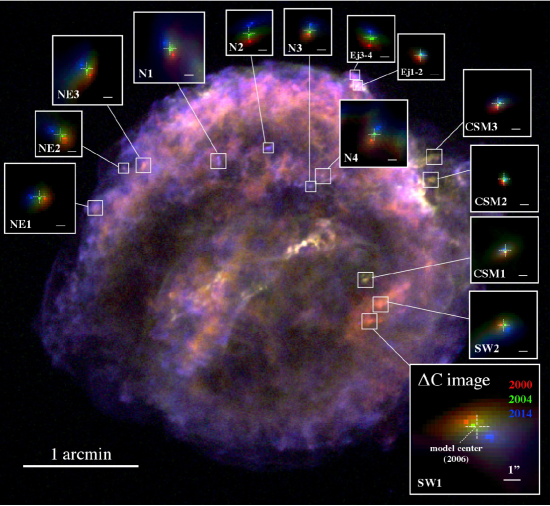
Figure 1.— Three-color image of Kepler’s SNR from the 2006 data set with red, green and blue images taken from the bands containing Fe L-shell emission (0.72-0.9 keV), O-Ly$\alpha$ emission (0.6–0.72 keV), and Si-He$\alpha$ emission (1.78-1.93 keV), respectively. The image is binned by 0.246^′′ and has been smoothed with a Gaussian kernel with $\sigma=0.492^{\prime\prime}$. The intensity scale is square root. White boxes show the regions used for the proper motion analysis. Small frames around the figure show $\Delta C$ images from the image fits. The pure red, green and blue colors show fitting results of each knot’s proper motion comparing the 2006 image to data from 2000, 2004 and 2014, respectively. The center position of each knot in the 2006 image is noted with the plus sign in each small frame, along with a 1^′′ scale bar in the lower right corner. The brightest pixel in each color in the insert frames shows the minimum $C$ value for that epoch; the range of $C$ values plotted in each frame was adjusted to enhance visibility. We alert the reader to the different uses of color in this figure: the main panel uses color to show spectral variations with position in Kepler’s SNR while the 14 insert panels use color to denote proper motions, showing fit results for the 3 different epochs with different colors.

Bandiera (1987) first connected the environmental characteristics of Kepler’s SNR, unusual for its location a few hundred pc above the Galactic plane, with the possibility of a high-speed ($\sim$300 km s^-1), mass-losing progenitor star. In his model, wind material is compressed by the low density ambient medium forming a dense bow shock in the direction of motion (toward the northwest). This produces a strong brightness gradient in X-ray and radio images and high density knots in the resulting SNR (see, e.g., Borkowski et al. 1992 for an early 2D hydro bow-shock model for the remnant). Bandiera’s model is likewise consistent with X-ray expansion measurements (Vink, 2008; Katsuda et al., 2008) that show slower expansion rates in the north compared with the rest of the remnant. More recent multi-dimensional hydrodynamical models (Velázquez et al., 2006; Chiotellis et al., 2012; Burkey et al., 2013; Toledo-Roy, Esquivel, Velázquez, & Reynoso, 2014) have considered a single degenerate (SD) scenario for the progenitor to Kepler’s SNR with the mass loss coming from the donor companion star to the white dwarf that exploded. However, it is important to note that no surviving red giant, AGB or post AGB donor star has been found in the central region of Kepler’s SNR (Kerzendorf et al., 2014).

In this article, we report three-dimensional space velocities of several X-ray knots in Kepler’s SNR determined from both proper motions and radial velocities using archival Chandra observations. Our results yield insights on the nature of the explosion and the ambient medium around Kepler’s SNR. In §2 we present the observational results from image and spectral analysis of the several knots, including measurements of elemental composition in addition to velocity. The discussion section (§3) studies the kinematics of the knots; reports a new, accurate, kinematic center for Kepler’s SNR; assesses the implications of these results on the evolutionary state and nature of the ambient medium; and reexamines the question of a possible left-over companion star under the SD scenario for the explosion. The final section summarizes the article. Uncertainties are quoted at the 1$\sigma$ (68.3%) confidence level unless otherwise indicated; positions are given in equinox J2000 throughout.

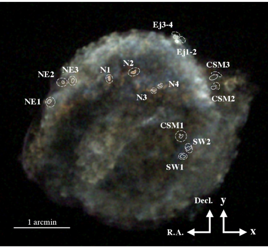
Figure 2.— Three-color image showing the Doppler velocities of Kepler’s SNR in the Si-He$\alpha$ line from the 2006 Chandra ACIS-S observation. The red, green and blue images come from the 1.78–1.83 keV, 1.84–1.87 keV, and 1.88–1.93 keV bands. Each image is smoothed with a Gaussian kernel with $\sigma=0.738^{\prime\prime}$ Solid lines show the regions used for the spectral analysis and dashed curves show the background regions.

2. Observational Results

The Chandra Advanced CCD Imaging Spectrometer Spectroscopic-array (ACIS-S, Garmire et al., 1992; Bautz et al., 1998) observed Kepler’s SNR four times: in 2000 (PI: S. Holt), 2004 (PI: L. Rudnick), 2006 (PI: S. Reynolds) and 2014 (PI: K. Borkowski). The total net exposure time for each of these observations is 48.8 ks, 46.2 ks, 741.0 and 139.1 ks, respectively. The time differences with respect to the long observation in 2006 are 5.96 yr (2000-2006), 1.64 yr (2004-2006) and 7.90 yr (2006-2014). We reprocessed all the level-1 event data, applying all standard data reduction steps with CALDB version 4.7.2, using a custom pipeline based on “chandra_repro” in CIAO version 4.8.

Serendipitous point sources were used to align the images. Sources were identified in each ObsID using the CIAO task wavdetect and position offsets were computed with wcs_match. All ObsIDs were matched to ObsID 6175, which was chosen as the reference because it has the longest exposure time (159.1 ks). At least 4 and as many as 17 sources, depending on ObsID, were used for the alignment. The source positions showed mean shifts in R.A. and decl. of less than 0.35^′′. Using the shift values, we updated the aspect solution of the event file using wcs_update. After corrections, the average residuals in the point source positions relative to the reference ObsID (#6175) are $<$0.25^′′.

2.1. Proper Motions of the Knots

Figure 1 shows a three-color image of Kepler’s SNR from the third epoch observation (in 2006) after image alignment, highlighting emission from primarily O-Ly$\alpha$ (green), Fe L-shell (red), and Si-He$\alpha$ (blue). Regions of CSM emission in Kepler’s SNR (e.g., CSM1–3 in the figure) tend to appear greenish in this figure due to relatively more emission from O. Ejecta knots appear as purple (both strong Si and Fe emission, e.g., N and NE knots) or orange (weaker Si to Fe, e.g., SW knots). Some of the purplish colored regions around the edge of the SNR contain strong nonthermal emission.

Figure 2 shows a Doppler velocity map of Kepler’s SNR made using three narrow energy bands in the Si-He$\alpha$ line. Our recent work on Tycho’s SNR (Sato & Hughes, 2017) demonstrated the ability of the Chandra ACIS instrument to measure radial velocities for relatively large and diffuse ejecta knots. The radial velocities of knots in Tycho’s SNR show an obvious pattern indicative of a spherically expanding shell—with the highest speeds through the center and decreasing speeds towards the limb. This pattern is not seen in Kepler’s SNR where instead the highest speeds (both red- and blue-shifted) appear as distinct knots lying in chains that stretch east-west in specific locations largely across the northern half of the remnant. A number of these knots (the N, NE, and SW sets) also showed large proper motions when comparing the images taken in 2000 and 2014 (see Fig. 3). We also identified three CSM knots and the northwest ejecta knots (Ej1, 2, 3, and 4, which we combined into two separate knots Ej1-2, Ej3-4) whose proper motions were recently measured with the Hubble Space Telescope (HST; Sankrit et al., 2016). None of the N, NE, and SW knots showed any evidence for optical emission in the HST images, while the CSM and Ej knots all did. We selected 14 knots for proper motion and radial velocity analyses.

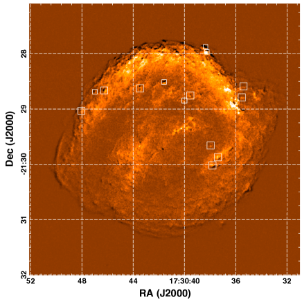
Figure 3.— Difference image made by subtracting the two Chandra observations of Kepler’s SNR taken in 2014 and 2000. White boxes show the regions used for the proper motion analysis.

To measure proper motions, we extracted image cut-outs about each knot for the 4 epochs. The image from the long observation in 2006 was used as the fitting model for each knot and was shifted in R.A. and decl. to obtain the 2D proper motion shifts. We employed the C-statistic, a maximum likelihood statistic for Poisson distributed data (Cash, 1979),

$$C=-2\Sigma_{i,j}(n_{i.j}~{}{\rm ln}~{}m_{i,j}-m_{i,j}-~{}{\rm ln}~{}n_{i.j}!)$$ (1)

where $n_{i,j}$ are the counts in pixel (i,j) of the image in each epoch, and $m_{i,j}$ are the model counts from the 2006 image scaled by the relative number of total counts (over the 0.6–2.7 keV band) from the entire SNR. We estimate the errors on the proper motion shifts using $\Delta C=C-C_{\rm min}$, which is similar to $\chi^{2}$ (Cash, 1979). The fitting errors are subdominant to the systematic errors in image alignment, which we determine by fitting the positions of seven serendipitous point sources using the same method. The systematic errors ($\sigma_{\rm x}$, $\sigma_{\rm y}$) are estimated to be (0.17^′′, 0.18^′′) for 2000, (0.26^′′, 0.20^′′) for 2004 and (0.21^′′, 0.32^′′) for 2014.

Images of $\Delta C$ for each knot are shown in small frames on Figure 1, clearly indicating the high proper motion of the ejecta knots, and Table 1 presents numerical results. We obtained acceptable fits for all knots (reduced $C$ = 0.95–2.04). For the NE, N and SW sets, we found large proper motions ($\sim$0.08–0.14^′′ yr^-1), comparable to values from around the rim (0.076–0.302^′′ yr^-1; Katsuda et al., 2008). In contrast, the CSM knots have small proper motions ($\lesssim$ 0.04^′′ yr^-1), consistent with being either ejecta knots significantly decelerated by interaction with the CSM or features in the ambient medium overrun by the forward shock. Our X-ray proper motion of the Ej3-4 knot is consistent with the H$\alpha$ result ($\sim$0.08–0.112^′′ yr^-1; Sankrit et al., 2016), but the proper motion of knot Ej1-2 is smaller by about a factor of two in the X-rays than in H$\alpha$ (0.069–0.083^′′ yr^-1). Knot Ej3-4 is detached from the main shell of X-ray emitting ejecta (and relatively distant from any slow moving optical knots); the agreement between the Chandra and HST proper motions indicates that the X-ray knot is driving the arc-shaped H$\alpha$ shock here. X-ray knot Ej1-2, however, is closer to the (slower moving) main ejecta shell and is partially superposed on bright optical radiative knots that appear to be slowly moving. We suspect that the discrepancy between the motion of the H$\alpha$ shock and knot Ej1-2 is due to some contamination of the X-ray knot by slower moving ejecta from the main shell or X-ray emission associated with the optical radiative knots.

Table 1Proper Motions and Radial Velocities of Knots in Kepler’s SNR

	Imaging Analysis				Spectral Analysis
	center of the model frame (epoch 2006)	mean sift: $\Delta$x, $\Delta$y	proper motion	angle	radial velocity	$\chi^{2}_{\nu}$ (d.o.f)
id	R.A., Decl. (J2000)	(arcsec yr-1)	(arcsec yr-1)	(degree)	(km s-1)
NE1	17h30m48s.022, $-21^{\circ}$29′01′′.87	$-0.112\pm$0.020, $+0.018\pm$0.019	0.112$\pm$0.020	81$\pm$10	$+$3170${}^{+50}_{-200}$	1.05 (320)
NE2	17h30m46s.963, $-21^{\circ}$28′41′′.21	$-0.099\pm$0.021, $+0.064\pm$0.020	0.117$\pm$0.021	57$\pm$10	$+$6540${}^{+890}_{-570}$	0.92 (166)
NE3	17h30m46s.224, $-21^{\circ}$28′39′′.74	$-0.064\pm$0.020, $+0.081\pm$0.020	0.103$\pm$0.020	38$\pm$11	$+$2970${}^{+210}_{-220}$	1.26 (297)
N1	17h30m43s.428, $-21^{\circ}$28′37′′.47	$-0.063\pm$0.020, $+0.088\pm$0.020	0.108$\pm$0.020	36$\pm$11	$+$8700${}^{+650}_{-470}$	0.96 (258)
N2	17h30m41s.561, $-21^{\circ}$28′30′′.59	$+0.008\pm$0.020, $+0.141\pm$0.019	0.141$\pm$0.019	357$\pm$8	$+$9110${}^{+30}_{-110}$	1.32 (259)
N3	17h30m39s.974, $-21^{\circ}$28′50′′.75	$+0.029\pm$0.020, $+0.076\pm$0.020	0.081$\pm$0.020	339$\pm$14	$+$5880${}^{+690}_{-1750}$	0.82 (165)
N4	17h30m39s.516, $-21^{\circ}$28′45′′.34	$+0.048\pm$0.021, $+0.099\pm$0.020	0.110$\pm$0.020	334$\pm$11	$+$10020${}^{+1270}_{-440}$	0.86 (192)
SW1	17h30m37s.788, $-21^{\circ}$30′01′′.09	$+0.101\pm$0.021, $-0.060\pm$0.020	0.118$\pm$0.020	239$\pm$10	$-$5590${}^{+340}_{-260}$	1.01 (253)
SW2	17h30m37s.366, $-21^{\circ}$29′52′′.23	$+0.068\pm$0.020, $-0.041\pm$0.020	0.079$\pm$0.020	239$\pm$14	$-$8000${}^{+500}_{-150}$	1.24 (297)
CSM1	17h30m37s.930, $-21^{\circ}$29′39′′.44	$-0.005\pm$0.020, $+0.022\pm$0.019	0.023$\pm$0.019	14$\pm$49	$+$740${}^{+980}_{-490}$	1.14 (191)
CSM2	17h30m35s.498, $-21^{\circ}$28′47′′.31	$+0.028\pm$0.020, $+0.023\pm$0.019	0.037$\pm$0.019	309$\pm$30	$-$2300${}^{+240}_{-280}$	1.19 (227)
CSM3	17h30m35s.366, $-21^{\circ}$28′35′′.31	$+0.021\pm$0.020, $+0.039\pm$0.019	0.044$\pm$0.019	332$\pm$26	$+$574${}^{+7}_{-90}$	1.26 (309)
Ej1-2	17h30m38s.222, $-21^{\circ}$27′57′′.92	$+0.028\pm$0.020, $+0.026\pm$0.019	0.038$\pm$0.019	313$\pm$29	$+$244${}^{+46}_{-10}$	1.42 (445)
Ej3-4	17h30m38s.328, $-21^{\circ}$27′52′′.51	$+0.010\pm$0.020, $+0.112\pm$0.019	0.112$\pm$0.019	355$\pm$10	$+$351${}^{+19}_{-22}$	1.69 (395)

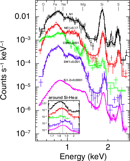
Figure 4.— Observed spectra and best fitting models for several knots in Kepler’s SNR (black: N1, red: NE1, green: CSM1, blue: SW1, magenta: Ej1-2). Although we only show the spectra from the 2006 data set here, spectra from all four epochs were used to constrain the model in the joint fit. The inset plots the spectra in the vicinity of the Si line, with an expanded energy scale, in order to illustrate the Doppler shifts.

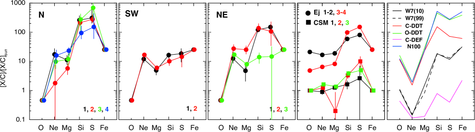
Figure 5.— Plots of the relative abundances of various elemental species with respect to carbon relative to solar ratios for the several sets of knots studied here. The rightmost panel shows, for comparison, the integrated yields from a variety of SN Ia explosion models including W7(99): W7 from Iwamoto et al. (1999); W7(10): W7 from Maeda et al. (2010); C-DEF: spherically symmetric pure-deflagration, C-DDT: delayed detonation after a spherical deflagration, and O-DDT: delayed detonation after an extremely offset deflagration all from Maeda et al. (2010); and N100: delayed detonation after a deflagration initiated at 100 ignition spots from Seitenzahl et al. (2013).

2.2. X-ray Spectroscopy of the Knots

We extracted spectra in each epoch (2000, 2004, 2006 and 2014) from the knot and background regions defined in Figure 2, accounting for position shifts due to the proper motion. The spectra were fitted in the 0.6–2.8 keV band using an absorbed vvnei + power-law model in XSPEC 12.9.0 (AtomDB v3.0.3). An additional Gaussian model was included to account for a feature at $\sim$1.2 keV from missing Fe-L lines in the atomic database (Brickhouse et al., 2000; Audard et al., 2001). Among the four spectra from the different epochs for each knot, fitted model parameters (temperature, ionization age, abundances, and radial Doppler velocity) were linked. Our spectral fits explicitly allow the ionization timescale, temperature, and redshift to be free parameters, so line centroid variations due to changes in the thermodynamic state are explicitly included in our fits, the derived values, and the uncertainty on the fitted redshift. To reduce the complexity of our fits, we fixed a number of our model parameters to the best-fit values determined by Katsuda et al. (2015). Specifically we fixed the column density to the value $N_{H}=6.4\times 10^{21}$ cm^-2 using the abundance table from Wilms et al. (2000) and the photon index of the power-law model to 2.64, allowing the normalization parameter to be free. We assumed no H and He in the shocked SN Ia ejecta (for the N, NE, SE and Ej knots), and fitted the Ne, Mg, Si and S abundances as free parameters. We fixed the abundances of [O/C]/[O/C]_⊙, [Ar/C]/[Ar/C]_⊙, [Ca/C]/[Ca/C]_⊙ and [Fe/C]/[Fe/C]_⊙ to be 0.46, 37, 67.41 and 25.28, respectively. For the Ej knots, we had to thaw the O abundance to obtain good fits. Our fits for these knots also showed more neon and magnesium emission compared to the other ejecta knots, implying that the Ej knots show a mix of both ejecta and CSM components. For the CSM knots, we used only an absorbed vvnei model. Here we include hydrogen and helium in the plasma, and fixed the abundances of He, C, O, Ar, Ca and Fe to the solar values. The nitrogen abundance is fixed to [N/H]/[N/H]${}_{\odot}=3.5$ as expected for the N-rich CSM of Kepler’s SNR, while the Ne, Mg, Si and S abundances are allowed to be free parameters. Figure 4 shows example spectra and best fitting models; the small insert figure shows the clear effect of the Doppler shifting on the Si-line of the knot spectra.

The first four panels of figure 5 plot the abundances of the various knots from our spectral fits. The abundances of all the N knots plus NE1 and NE2 are quite similar and show strong enhancements of Si and S compared to Fe as well as the lighter elements. This is also the case for the Ej knots, but with less contrast between Si/S and the other species. The SW knots plus NE3 appear to follow a different abundance pattern, while the CSM knot abundances are close to the solar ratios for Ne and Mg, but show some enhancement (by factors of a few) in Si and S (albeit with large uncertainties). The last panel of this figure shows integrated yields from a variety of published SN Ia explosion models (see the figure caption for details and citations) that indicate that the ejecta knot abundances we find are broadly consistent with theoretical expectations. However, it is highly unlikely that the knots should contain material with the spatially integrated yields, but rather they should reflect the composition of the location in the exploding white dwarf where they were formed. Indeed the high abundances of Si and S relative to Fe (especially for NE1 and NE2 and the N knots) indicate that these knots formed at the outer, partially burned layer of the exploding white dwarf. The presence of Fe and low O abundance further restrict their origin to the partial Si-burning regime (e.g., mass coordinate range of 0.7–0.9 $M_{\odot}$ in W7, Nomoto et al. 1984). A future study will use the fitted abundances in more detail to better identify where these knots formed in the explosion.

Our fits are able to accurately represent the various knot spectra across the range of significant compositional differences we obtain. We also find that the best-fitting electron temperatures ($kT_{\rm e}$) and ionization ages ($n_{\rm e}t$) differ from knot to knot ($kT_{\rm e}\sim 0.2-1$ keV, $n_{\rm e}t\sim 7\times 10^{9}-5\times 10^{11}$ cm³ s). In some cases these are correlated in interesting ways. For example the O abundance and ionization age in knot Ej1-2 are larger than those in the adjacent Ej3-4 knot: [O/C]/[O/C]${}_{\odot}=19-23$ and $n_{\rm e}t=(1.5-1.6)\times 10^{11}$ for Ej1-2, [O/C]/[O/C]${}_{\odot}=4-5$ and $n_{\rm e}t=(5.9-6.9)\times 10^{10}$ for Ej3-4. These spectral results argue for a significant CSM interaction for knot Ej1-2, in agreement with the argument put forward above to explain the proper motion differences.

Radial velocity determination can be sensitive to the background subtraction. To test this, we replaced the individual local background regions with an annular ($r=2.4^{\prime}$–$3.5^{\prime}$) blank sky region surrounding the remnant. The spectral fits were as good, but the precise values of the measured speeds differed, on average, by $\sim$1,500 km s^-1 with the local background results being higher than the blank sky background in nearly all regions (exceptions were the CSM and Ej regions). This trend is expected because using local background regions removes contaminating emission with a different velocity (from, e.g., the other hemisphere of the remnant) projected across the knot spectral extraction region. Such contamination tends to reduce a knot’s observed speed compared to its actual speed.

The numerical accuracy of our velocity measurements with the ACIS-S detector is limited by ACIS gain calibration uncertainties. For example, Sato & Hughes (2017) showed a discrepancy in the radial velocity measurements of $\sim$500–2,000 km s^-1 between the ACIS-S and ACIS-I detectors for a set of knots similar to those we study here, which we argued was likely a result of uncertain gain calibration. Still, the large velocities we measure for most knots ($>$ 5,000 km s^-1) remain significant even given the level of systematic uncertainty due to instrumental effects mentioned here and background subtraction discussed in the previous paragraph.

The two rightmost columns of Table 1 summarize the radial velocity fits. The N and SW knots have high radial speeds (5,590 km s^-1 $<v<$ 10,020 km s^-1) that are $\sim$2–3 times higher than the ejecta knot speeds quoted by Sankrit et al. (2016) from HST proper motions: $\sim$ 1,600–3,000 km s^-1. On the other hand, the CSM and Ej knots show relatively low speeds ($<$ 2,300 km s^-1).

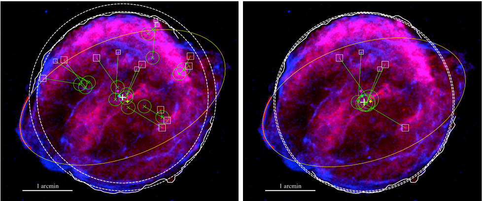
Figure 6.— Two-color image of the 0.6–2.7 keV band (red) and the 4.2–6 keV band (blue). Left: Extrapolation of the measured proper motion vector for each knot back to the explosion date (1604 Oct 9), assuming purely undecelerated motion. The green lines, crosses and circles show the estimated distance moved, best-fit extrapolated original position and 1 $\sigma$ uncertainty. Five knots (N1, N2, N3, N4 and SW1) extrapolate back to a consistent position which we note by the solid white cross symbol (whose size denotes the 1 $\sigma$ uncertainty). The other cross symbols denote expansion centers estimated by others: cyan (radio: Matsui et al., 1984), magenta and yellow (X-ray: Katsuda et al., 2008; Vink, 2008). Two dashed circles, centered on the position we determine here, match the northern ($r=1.71^{\prime}$) and southern ($r=1.87^{\prime}$) extent of Kepler’s SNR. The yellow ellipse is centered on the kinematic center, while the axis lengths and orientation are matched to the nonthermal filament on the eastern rim (highlighted with red crosses). Right: In this panel, we use only the five knots with the highest expansion indices to extrapolate back to the explosion center including the effects of deceleration using the measured expansion index. The agreement between the individual knots is greatly improved. The dynamical center here is shifted by about 6^′′ south of the center shown in the left panel.

3. Discussion

3.1. Undecelerated Ejecta Knots and the Kinematic Center of Kepler’s SNR

Given the known age of Kepler’s SNR ($401.7$ yr at the mean time of the third epoch observation) we can use our proper motion vectors to extrapolate the position of each knot back to its location at the time of explosion. Initially, we assume that each knot moves without any deceleration. Figure 6 (left panel) shows the 2006 locations (small boxes), the distance traveled (green lines) and the initial locations in 1604 (green circles) of each of the knots. Five knots extrapolate back to a consistent position (for values see Table 2), which we identify as the kinematic center of the explosion. This result agrees well with other estimates for the explosion center, but, since it relies on knots that are nearly undecelerated, it is much less sensitive to systematic errors due to the spatial variation of the expansion rate across Kepler’s SNR. We use our kinematic center to determine the expansion index ($m$ in the relation $r\propto t^{m}$) as $m=\mu\times t/r$, which depends only on each knot’s measured proper motion ($\mu$), its distance from the expansion center ($r$) and the remnant’s age ($t$). The expansion indices (see Fig. 7) range from low values, $m<0.25$, indicating significant deceleration to high values, $m>0.75$, indicating little to no deceleration.

For a power-law evolution of radius with time as we use here, it is possible to estimate the effects of deceleration on the distance traveled by the knot and thereby obtain a more accurate estimate for the kinematic center. We assume that the expansion index is constant with time, which is only a good approximation for knots with high expansion indices; so we restrict our analysis to the same five knots introduced in the preceding paragraph. We integrate the time evolution of velocity $v=v_{f}(t/t_{f})^{m-1}$ over the age of the SNR ($t_{f}$) to obtain the simple result for the distance traveled: $r=v_{f}t_{f}/m$. We start with the results from the previous paragraph, which yielded a kinematic center and an estimate of $m$ for each knot. The distance each knot has moved is now redetermined assuming decelerated motion according to its $m$ value (although $m$ was restricted to values of 1 or less) and the equation introduced a few lines above. Averaging these values leads to a new estimate for the kinematic center. This process was iterated until the individual $m$ values and the location of the kinematic center converged, which took about 30 iterations. The kinematic center shifts slightly south from the case of undecelerated motion above (see Table 2), but the difference between the two estimates is not highly significant, only $\sim$1 $\sigma$ ($\sim 6^{\prime\prime}$). Note how the $m$ values have changed only slightly as well.

Table 2Kinematic center of Kepler’s SNR from high speed knots

	Undecelerated	Decelerated
Parameter	($r=v_{f}t_{f}$)	($r=v_{f}t_{f}/m$)
Kinematic center
R.A.	17h30m41s.189	17h30m41s.321
Decl.	$-21^{\circ}$29′24′′.63	$-21^{\circ}$29′30′′.51
$\sigma_{\rm RA}$, $\sigma_{\rm Dec}$	$\pm 3.6^{\prime\prime}$, $\pm 3.5^{\prime\prime}$	$\pm 4.4^{\prime\prime}$, $\pm 4.3^{\prime\prime}$
Expansion indices and offsets (′′) from kinematic center
	$m$, x, y	$m$, x, y
Knot N1	0.76, $-$12.4, $+$24.2	0.71, $+$12.3, $+$7.0
Knot N2	1.04, $-$17.6, $\phantom{0}-$5.1	0.95, $-$14.3, $+$0.2
Knot N3	0.87, $+$10.1, $\phantom{0}+$7.5	0.75, $\phantom{0}+$5.8, $-$1.2
Knot N4	0.97, $\phantom{0}+$8.2, $\phantom{0}-$0.9	0.86, $\phantom{0}+$4.9, $-$1.6
Knot SW1	0.80, $+$13.5, $-$24.7	0.83, $\phantom{0}+$0.2, $-$2.5
RMS x,y offsets	12.8, 16.0	9.1, 3.4
Overall radius of Kepler’s SNR from kinematic center
Radius to N (′)	$1.71\pm 0.04$	$1.77\pm 0.03$
Radius to S (′)	$1.87\pm 0.04$	$1.80\pm 0.04$

Combining the proper motions and radial velocities allows us to determine the 3-dimensional (3D) space velocities of these X-ray knots. The distance to Kepler’s SNR is not well known with estimates ranging from $\sim$4.0 kpc to $>$ 7 kpc; here we use a value of 5 kpc which is consistent with H I absorption measurements (Reynoso & Goss, 1999) and recent optical proper motion measurements of Balmer shocks (Sankrit et al., 2016). Figure 7 presents the scatter plot of 3D space velocity versus expansion index. There is a clear trend for low space velocity knots to have small expansion indices, while the high space velocity knots tend to have large expansion indices. It is notable that the three knots with the highest space velocities also have large expansion indices; for these specific knots we determine space velocities of 9,100 km s^-1 $\lesssim v_{\rm 3D}\lesssim$ 10,400 km s^-1 and expansion indices of 0.75 $\lesssim m\lesssim$ 1.0. Thus not only are these knots expanding at nearly the free expansion rate, they are moving with space velocities that are comparable to the expansion speed of Si ejecta in SN Ia near maximum brightness (10,000–12,000 km s^-1, see Filippenko, 1997, and references within).

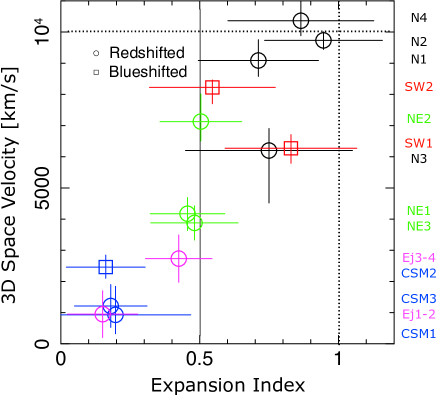
Figure 7.— Scatter plot between 3D space velocity and expansion index for the 14 knots identified in Fig. 1. The space velocity is the root-sum-square combination of the radial velocity and the proper motion assuming a distance of 5 kpc to Kepler’s SNR. The plotted uncertainties are at the 90% confidence level. The different knots are indicated with different colored symbols and are labeled along the right side. Circles (boxes) indicate redshifted (blueshifted) knots. The solid vertical line shows the average expansion index for the remnant ($r\propto t^{0.5}$: Vink, 2008).

We can also estimate the 3D radial locations of the knots using each knot’s current projected distance from the kinematic center and the angle defined by the radial and transverse (proper motion) speeds. The angle obviously depends on the remnant’s distance. As a reference for comparison, we use the maximum projected extent of Kepler’s SNR from the kinematic center, which is $\sim$2.3^′ (3.35 pc for a distance of 5 kpc); this occurs at the northwest protuberance. A knot moving with a constant speed of 10,000 km s^-1 would reach a radius of 4.1 pc in the lifetime of Kepler’s SNR, and this radius would be equal to the remnant’s maximum projected extent for a distance of 6.1 kpc. For the fastest moving knots (N1, N2, and N4), the estimated 3D radial locations are 1.57, 1.26, and 1.48 times the maximum projected extent assuming a distance of 5 kpc. Values are larger than the simple example given because these knots have suffered some deceleration. For a distance of 7 kpc, the radial locations are 1.16, 0.95, and 1.09, respectively, times the maximum projected extent. These considerations tend to favor distances to Kepler’s SNR on the larger range of those reported.

There are interesting relationships between the elemental composition of the knots and their space velocities and inferred extent of deceleration. The N series of knots show both high speed and low deceleration ($m>0.5$), along with a clear ejecta-dominant composition showing high Si and S abundances (Fig. 5). Although the knots NE1 and NE2 show similar abundances, they appear to have been decelerated more ($m\approx 0.5$) and are currently moving more slowly. The SW knots are kinematically similar to the N knots, but are noticeably different in composition. On the other hand, the CSM and Ej knots have low space velocities ($v_{\rm 3D}<$ 3,000 km s^-1) together with small expansion indices ($m<$ 0.5) and have relatively less contrast between their light (O, Ne, Mg) and heavy (Si, S, Fe) element abundances. Based on the abundance patterns, the CSM knots appear to be dominated by the ambient medium while the Ej knots are more dominated by ejecta.

3.2. Global Evolution of Kepler’s SNR

The mean expansion index of Kepler’s SNR from published studies using high resolution Chandra images is $m\sim 0.5$ with evidence for higher rates of expansion in the south compared to the north (e.g., Katsuda et al., 2008; Vink, 2008). The dashed circles plotted in Fig. 6 are centered on our new kinematic center for either undecelerated (left panel) or decelerated (right panel) motion and were chosen to match the northern and southern extents of the SNR. The north/south radii (numerical values given in Table 2) differ by $9^{+5}_{-4}$ % for undecelerated motion (left) and $2\pm 4$ % for decelerated motion (right), where the uncertainties were estimated from the standard deviation of the radial scatter of the plotted contour about the estimated best-fit circle.

Chiotellis et al. (2012) calculated models for Kepler’s SNR assuming the progenitor system was a symbiotic binary (a white dwarf and a 4-5 $M_{\odot}$ AGB star) moving toward the northwest with a velocity of 250 km s^-1. As in the model of Bandiera (1987), this produces an asymmetric wind around the progenitor with the densest regions at the stagnation point (i.e., where the momentum of the wind and ambient medium equilibrate) ahead of the star in the direction of motion. In their model A, which provides a decent description of Kepler’s SNR, the forward-shock interaction with the wind bubble begins $\sim$300 yr after the explosion when the forward shock was at a radius of $\sim$2.7 pc. This encounter has a strong, immediate, effect on the expansion index in the direction toward the wind-stagnation point where the dense shell material causes the forward shock to decelerate quickly. With time, the radial asymmetry of the remnant also grows, but the decrease of the expansion index is more immediate and dramatic.

As seen in Fig. 7 in Chiotellis et al. (2012), the expansion index $m$ at the stagnation point changes quickly from a value of $\sim$0.8 to $\sim$0.45 during the first $\sim$30 yr after the encounter, while the expansion in the opposite direction remains high. Over the same time frame the remnant radius in the direction of the stagnation point grows more slowly so that the remnant starts to become asymmetric, but the difference of the radii is not so large ($\lesssim$2%). Thus this model is consistent both with the large north-south variation of expansion index observed in Kepler’s SNR ($m=$ 0.47–0.83: Katsuda et al., 2008) and the modest north-south radius difference as shown in Fig. 6 (right).

In addition, we find that the bilateral protrusions at the southeast/northwest rims match well with a simple elliptical geometry (plotted as the yellow figures in Fig. 6). In each panel the ellipse is centered on the kinematic center for undecelerated (left) or decelerated (right) knot motion and the axis lengths and orientation are matched to the shape of the nonthermal filament on the eastern rim. Although the physical origin of these prominent structures is not yet resolved, there have been suggestions that the symmetric protrusions are related to the explosion (e.g., Tsebrenko & Soker, 2013). If so, the notable agreement of the shape and orientation of the protrusions to a simple elliptical geometry centered on and symmetric about the kinematic center derived from the decelerated knot motions, offers further support for this being the site of the explosion.

3.3. Spatial Density Variations in the Ambient Medium

In one-dimensional SNR evolutionary models, a high value of the expansion parameter indicates that the remnant is interacting with a low density ambient medium. Here we derive an estimate of the density required. Dwarkadas & Chevalier (1998) investigated the dynamical evolution of SN Ia assuming an exponential ejecta density profile. An expansion parameter $m\gtrsim$ 0.75 is realized in their models at a scaled time of $t^{\prime}\lesssim$ 0.1 (see Fig. 2f in their paper). The scaled time is related to the pre-shock ambient medium density ($n_{\rm H}$), and the remnant’s age, explosion energy ($E_{51}$ in units of $10^{51}$ ergs), and ejected mass ($M_{\rm ej}$) as

$$n_{\rm H}\approx 0.24\,(t^{\prime})^{3}\,E_{51}^{-3/2}(M_{\rm ej}/M_{\rm ch})^{5/2}\,{\rm cm}^{-3}$$

for the remnant’s age of 401.7 yr. Assuming typical values for the explosion energy ($E_{51}=1$) and ejected mass ($M_{\rm ej}=M_{\rm ch}=1.4\,M_{\odot}$), allows us to convert the scaled time for nearly undecelerated motion to an upper-limit on the ambient medium density (assumed uniform) of $n_{\rm H}<2.4\times 10^{-4}$ cm^-3. This value is comparable to the expected density at the remnant’s location above the Galactic plane in the absence of stellar mass loss.

However, a compact knot, overdense with respect to its surroundings, undergoes a considerably different type of evolution than does an idealized spherically symmetric distribution of ejecta. To investigate this scenario, we follow Wang & Chevalier (2001) who simulated the evolution of clumped ejecta in Tycho’s SNR to understand the conditions under which an ejecta knot could survive as it propagates out to, and possibly deforms, the forward shock. In this scenario a compact ejecta knot enters the reverse shock at some time and propagates outward through the high-pressure zone of shocked ejecta. The impact of the reverse shock on the knot drives a transmitted shock into the knot crushing it; in time this shock exits the knot which sends a rarefaction wave through it. Meanwhile instabilities develop along the knot boundary due to shear flow and rapid local accelerations that result in the destruction of the cloud after a few cloud-crushing times. This key timescale is given by $t_{\rm cc}=\chi^{1/2}r_{\rm cloud}/v_{\rm shock}$ (Klein et al., 1994), where $\chi$ is the density contrast of the knot with respect to the intercloud medium, $r_{\rm cloud}$ is the initial radius of the cloud, and $v_{\rm shock}$ is the velocity of the shock in the intercloud medium. Note that this timescale was originally developed for the case of an interstellar cloud impacted by the forward shock of a SN explosion, but is applicable to the closely analogous knot/reverse shock situation we have here.

The survivability of an ejecta clump depends on its size (relative to the size of the high pressure shocked ejecta zone) and density contrast with respect to the rest of the ejecta. Smaller clumps with higher density contrast survive for longer. Moreover the drag on a high speed clump depends sensitively on the density contrast, in the sense that a higher density contrast produces relatively less drag. Wang & Chevalier (2001) therefore find that in order for there to be undecelerated clumps of ejecta near the limb of Tycho’s SNR some 400 year after explosion, the density contrast needs to be high, $\chi>100$.

However, another option for increasing the survivability of an ejecta knot is to have it interact with the reverse shock when that shock is still forming during its early evolutionary phase. For example Fig. 8 of Wang & Chevalier 2001 shows a knot that survives and continues expanding out to deform the forward shock from its initial interaction with the reverse shock at a scaled time of $t^{\prime}=0.217$ through to $t^{\prime}\sim 0.8$. The same scaling applies here as in the first paragraph of this section so a value of the scaled time of $\sim$0.8 corresponds to an ambient medium density of $n_{\rm H}\sim 0.1$ cm^-3. Such a low density would additionally allow for clumps with lower density contrast to survive to the current age. Thus, to summarize, the presence of undecelerated knots in Kepler’s SNR requires either that those knots were generated with a high initial density contrast ($\chi>100$) or that the ambient medium contains lower-density ($n_{\rm H}\sim 0.1$ cm^-3) windows or gaps through which potentially lower density contrast knots have propagated.

The evidence that Kepler’s SNR is embedded in a dense environment is strong. Yet our work now suggests that the ambient medium could be structured including both higher and lower density regions. One possibility, as briefly explored by Burkey et al. (2013), might be that the donor star’s wind has sculpted a dense disk-like structure with lower densities perpendicular to the disk plane. Another option could rely on an “accretion wind” from the accreting white dwarf (Hachisu et al., 1996), which has the potential to blow a large, low density cavity that allows for ejecta to expand rapidly (Badenes et al., 2007). If the progenitor system to Kepler’s SNR had a bipolar outflow (as in the case of the supersoft X-ray binary RX J0513.9–6951: Pakull et al., 1993; Hutchings et al., 2002), the ambient density along the polar axis could be much lower than elsewhere.

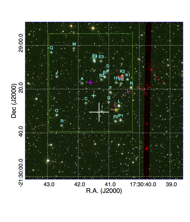
Figure 8.— Hubble Space Telescope color image of Kepler’s SNR using data from the Advanced Camera for Surveys (ACS) in the F502N (blue), F550M (green), and F660N (red) filters that trace [O III] $\lambda$ 5007 emission, the stellar continuum, and H$\alpha$, respectively. The green box is the region studied by Kerzendorf et al. (2014) where they measured spectra from the ground for a number of stars (not all of which were isolated). The 24 stars circled in cyan are those with V-band luminosities greater than $\sim$10$L_{\odot}$ at the distance of the remnant. Published explosion centers are shown with small magenta, cyan, and yellow plus signs (same as in Fig. 6). The kinematic center reported here is shown as the large white cross, the size of which denotes the 1$\sigma$ uncertainty.

3.4. Implications for the Left-Over Companion Star

Our new kinematic center allows us to reopen the search for a surviving donor star under the SD scenario for the progenitor to Kepler’s SNR. The most extensive study to date was carried out by Kerzendorf et al. (2014). These authors identified two dozen stars from HST with $V$-band luminosities greater than $\sim$10 $L_{\odot}$ assuming they lie at the distance of Kepler’s SNR. We indicate these stars on Fig. 8 with cyan colored circles. Kerzendorf et al. (2014) use ground-based optical spectroscopy to measure radial velocities for these stars, although some of the candidates (E, B, P, H, and K) were blended in the ground-based data, and in addition it was not possible to obtain a reliable radial velocity measurement for star I.

The radial velocities were compared to two velocity distributions: one for field stars based on the Besançon model (Robin et al., 2003) of galactic dynamics and the other based on the distribution of radial velocities for SD donors ranging from main-sequence to giant stars (Han, 2008). A probability was assigned to each star based on a Monte Carlo simulation. None of the stars were significant outliers with respect to the Besançon model, although a number were inconsistent with the expected donor distribution. Kerzendorf et al. (2014) consider candidates E1, E2, K1, L, and N to be the most notable for further follow-up, since they have $L>20L_{\odot}$ and a modest probability for being consistent with the expected radial velocity distribution for a donor star.

We can now assess the probability of positional agreement between the explosion center and each candidate. The 3-$\sigma$ limit on the allowed distance is 15^′′ to which we add 3.5^′′ to account for the donor’s possible proper motion ($<$200 km s^-1). Thirteen of the HST candidate stars fall within this area, including stars L (the most luminous candidate with $L_{V}=86L_{\odot}$), I (no radial velocity measurement), and G (second highest donor probability based on radial velocity), although the later two stars are of modest luminosity ($L_{V}=7L_{\odot}$ and 9$L_{\odot}$, respectively). Although there remains no obvious donor candidate for the traditional SD-scenario, our new kinematic center has ruled out many of the interesting candidates suggested for additional follow-up and has significantly reduced the search area for donor candidates for modified SD-scenarios (e.g., Di Stefano et al., 2011; Wheeler, 2012).

4. Conclusions

Most of our key results are based on the proper motion analysis of the four available epochs (from 2000 to 2014) of Chandra ACIS-S X-ray observations of Kepler’s SNR. We have discovered five X-ray–emitting knots with no detectable optical emission that are moving with nearly undecelerated motion (i.e., with expansion indices $>$ 0.75). The proper motion of these knots extrapolate back, over the age of the remnant, to a consistent and accurate center when their (modest) deceleration is included. A number of prominent structures in the remnant display a notable symmetry about the new kinematic center. For example the similarity between the northern and southern radii suggests that the forward shock of the remnant has encountered the northern density enhancement fairly recently, within the last 100 years or so, as some models argue (e.g., Chiotellis et al., 2012). The symmetric shape, extent and orientation of the southeast/northwest protrusions about the kinematic center add evidence to arguments that these protrusions may be related to the explosion process itself.

Our spectral analysis provides information on the composition of the knots. We report on three knots with near-solar abundances that show little proper motion or radial velocity. The Ej knots were selected because their associated H$\alpha$ shocks had measured proper motions from HST data (Sankrit et al., 2016). In the X-ray band these knots have metal-enhanced abundances but with a larger abundance of low-$Z$ species (O, Ne, Mg) compared to Si, S, and Fe than the other X-ray ejecta knots studied here. The Ej knots show high amounts of deceleration and low 3D velocities. Beyond this, however, there is no simple relationship between knot composition and motion. The N and NE series of knots share similar abundance patterns with high Si and S abundances, some Fe, and very low O abundances but have a range of expansion indices (from 0.45 to 0.95). On the other hand the SW knots show 3D speeds and expansion indices that fall between the NE and N knots, but their spectra show considerably less enhancement of the Si and S abundances compared to Fe. This strongly indicates that the origin of the knots (traced by composition) is independent of the kinematics of the knots (traced by the expansion index).

The measurement of radial velocities from spectral analysis of Chandra ACIS data is subject to systematic uncertainty from detector (gain uncertainty) and analysis (background subtraction) effects, so we summarize the key results from these measurements separately here. We find that the 3D space velocities of the highest speed knots are in the range 9,100 km s^-1 $\lesssim v_{\rm 3D}\lesssim$ 10,400 km s^-1, which is similar to the expansion speed of Si-rich ejecta seen in the optical spectra of SN Ia near maximum light. We also find a correlation between 3D speed and expansion index; the sense of the correlation is not surprising: higher speeds correlate with higher expansion indices and vice versus.

We looked into the conditions that would allow for the existence of high speed, undecelerated knots in Kepler’s SNR some 400 years after explosion, using the article by Wang & Chevalier (2001) as a useful guide. One option would require that the knots formed with a high density contrast (more than 100 times the density of the interknot medium); another would require that knots with potentially lower density contrast propagated through an ambient medium with a relatively low density ($<$0.1 cm^-3). We favor the latter interpretation since the generation of high-density-contrast clumps in a SN Ia explosion seems less plausible to us than the possibility that the environment of Kepler’s SNR contains gaps or windows of lower density gas.

Our new kinematic center has well-defined positional uncertainties which have allowed us to refine the search for possible surviving donor stars under the single-degenerate (SD) scenario for SN Ia. As shown before (Kerzendorf et al., 2014) there are no viable candidates for a traditional SD-scenario. Nevertheless our new position for the explosion center rules out several interesting candidates suggested by others for further follow-up and has greatly reduced the area to be searched for fainter donor stars under more exotic SD scenarios.

Our work has added new important pieces of evidence to the enigmatic remnant of Kepler’s SN that bear on both the nature of the explosion and the structure of the ambient medium. Further study of the detailed composition of the new high-speed ejecta knots should allow us to identify the conditions of the burning front where they formed during the explosion. Mapping the positions and velocities of other high-speed ejecta knots in Kepler’s SNR should allow us to determine the extent of the low density regions within the ambient medium. This will be important information for understanding the progenitor system.

References

- Audard et al. (2001) Audard, M., Behar, E., Güdel, M., et al. 2001, A&A, 365, L329
- Badenes et al. (2007) Badenes, C., Hughes, J. P., Bravo, E., & Langer, N. 2007, ApJ, 662, 472
- Bandiera (1987) Bandiera, R. 1987, ApJ, 319, 885
- Bautz et al. (1998) Bautz, M. W., Pivovaroff, M., Baganoff, F., et al. 1998, Proc. SPIE, 3444, 210
- Borkowski et al. (1992) Borkowski, K. J., Blondin, J. M., & Sarazin, C. L. 1992, ApJ, 400, 222
- Brickhouse et al. (2000) Brickhouse, N. S., Dupree, A. K., Edgar, R. J., et al. 2000, ApJ, 530, 387
- Burkey et al. (2013) Burkey, M. T., Reynolds, S. P., Borkowski, K. J., & Blondin, J. M. 2013, ApJ, 764, 63
- Cash (1979) Cash, W. 1979, ApJ, 228, 939
- Chiotellis et al. (2012) Chiotellis, A., Schure, K. M., & Vink, J. 2012, A&A, 537, A139
- Dennefeld (1982) Dennefeld, M. 1982, A&A, 112, 215
- Di Stefano et al. (2011) Di Stefano, R., Voss, R., & Claeys, J. S. W. 2011, ApJ, 738, L1
- Dwarkadas & Chevalier (1998) Dwarkadas, V. V., & Chevalier, R. A. 1998, ApJ, 497, 807
- Filippenko (1997) Filippenko, A. V. 1997, ARA&A, 35, 309
- Garmire et al. (1992) Garmire, G. P., Ricker, G. R., Bautz, M. W., et al. 1992, AIAA Space Program and Technologies Conference: The AXAF CCD Imaging Spectrometer (New York: AIAA)
- Hachisu et al. (1996) Hachisu, I., Kato, M., & Nomoto, K. 1996, ApJ, 470, L97
- Han (2008) Han, Z. 2008, ApJ, 677, L109
- Hughes & Helfand (1985) Hughes, J. P., & Helfand, D. J. 1985, ApJ, 291, 544
- Hutchings et al. (2002) Hutchings, J. B., Winter, K., Cowley, A. P., Schmidtke, P. C., & Crampton, D. 2002, AJ, 124, 2833
- Iwamoto et al. (1999) Iwamoto, K., Brachwitz, F., Nomoto, K., et al. 1999, ApJS, 125, 439
- Katsuda et al. (2008) Katsuda, S., Tsunemi, H., Uchida, H., & Kimura, M. 2008, ApJ, 689, 225-230
- Katsuda et al. (2015) Katsuda, S., Mori, K., Maeda, K., et al. 2015, ApJ, 808, 49
- Kerzendorf et al. (2014) Kerzendorf, W. E., Childress, M., Scharwächter, J., Do, T., & Schmidt, B. P. 2014, ApJ, 782, 27
- Klein et al. (1994) Klein, R. I., McKee, C. F., & Colella, P. 1994, ApJ, 420, 213
- Maeda et al. (2010) Maeda, K., Röpke, F. K., Fink, M., et al. 2010, ApJ, 712, 624
- Matsui et al. (1984) Matsui, Y., Long, K. S., Dickel, J. R., & Greisen, E. W. 1984, ApJ, 287, 295
- Nomoto et al. (1984) Nomoto, K., Thielemann, F.-K., & Yokoi, K. 1984, ApJ, 286, 644
- Pakull et al. (1993) Pakull, M. W., Motch, C., Bianchi, L., et al. 1993, A&A, 278, L39
- Reynolds et al. (2007) Reynolds, S. P., Borkowski, K. J., Hwang, U., et al. 2007, ApJ, 668, L135
- Reynoso & Goss (1999) Reynoso, E. M., & Goss, W. M. 1999, AJ, 118, 926
- Robin et al. (2003) Robin, A. C., Reylé, C., Derrière, S., & Picaud, S. 2003, A&A, 409, 523
- Sankrit et al. (2016) Sankrit, R., Raymond, J. C., Blair, W. P., et al. 2016, ApJ, 817, 36
- Sato & Hughes (2017) Sato, T., & Hughes, J. P. 2017, ApJ, 840, 112
- Seitenzahl et al. (2013) Seitenzahl, I. R., Ciaraldi-Schoolmann, F., Röpke, F. K., et al. 2013, MNRAS, 429, 1156
- Toledo-Roy, Esquivel, Velázquez, & Reynoso (2014) Toledo-Roy, J. C., Esquivel, A., Velázquez, P. F., & Reynoso, E. M. 2014, MNRAS, 442, 229
- Tsebrenko & Soker (2013) Tsebrenko, D., & Soker, N. 2013, MNRAS, 435, 320
- van den Bergh & Kamper (1977) van den Bergh, S., & Kamper, K. W. 1977, ApJ, 218, 617
- Velázquez et al. (2006) Velázquez, P. F., Vigh, C. D., Reynoso, E. M., Gómez, D. O., & Schneiter, E. M. 2006, ApJ, 649, 779
- Vink (2008) Vink, J. 2008, ApJ, 689, 231-241
- Wang & Chevalier (2001) Wang, C.-Y., & Chevalier, R. A. 2001, ApJ, 549, 1119
- Wheeler (2012) Wheeler, J. C. 2012, ApJ, 758, 123
- White & Long (1983) White, R. L., & Long, K. S. 1983, ApJ, 264, 196
- Williams et al. (2012) Williams, B. J., Borkowski, K. J., Reynolds, S. P., et al. 2012, ApJ, 755, 3
- Wilms et al. (2000) Wilms, J., Allen, A., & McCray, R. 2000, ApJ, 542, 914