A new method to unveil embedded stellar clusters

In this paper we present a novel method to identify and characterize stellar clusters deeply embedded in a dark molecular cloud. The method is based on measuring stellar surface density in wide-field infrared images using star counting techniques. It takes advantage of the differing $H$-band luminosity functions (HLFs) of field stars and young stellar populations and is able to statistically associate each star in an image as a member of either the background stellar population or a young stellar population projected on or near the cloud. Moreover, the technique corrects for the effects of differential extinction toward each individual star. We have tested this method against simulations as well as observations. In particular, we have applied the method to 2MASS point sources observed in the Orion A and B complexes, and the results obtained compare very well with those obtained from deep Spitzer and Chandra observations where presence of infrared excess or X-ray emission directly determines membership status for every star. Additionally, our method also identifies unobscured clusters and a low resolution version of the Orion stellar surface density map shows clearly the relatively unobscured and diffuse OB 1a and 1b sub-groups and provides useful insights on their spatial distribution.

1 Introduction

Embedded star clusters offer one of the best opportunities to understand star formation. Within these astrophysical laboratories hundreds of stars are formed in volumes below $1\mbox{ pc}^{3}$. Overall, it is estimated that 80%–90% of young stellar objects (YSOs) form in embedded clusters (Lada & Lada, 2003; although the exact fraction is somewhat sensitive to the definition of a cluster, see Bressert et al., 2010). It is now established that the fate of these objects is directly linked to the evolution of the molecular gas, which is responsible for most of the gravitational potential that binds the stars in the cluster. Therefore, it is important to study these objects in their early phases, before they are subject to infant mortality (Lada et al., 1984; Geyer & Burkert, 2001).

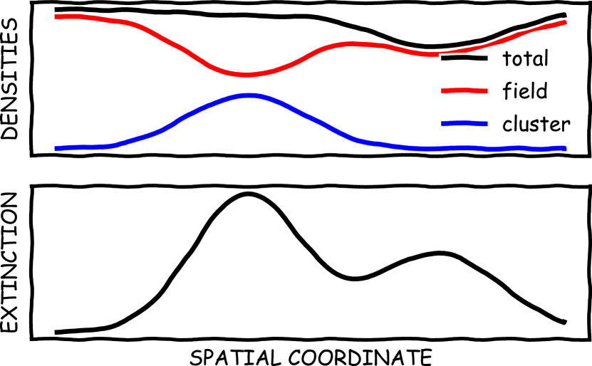
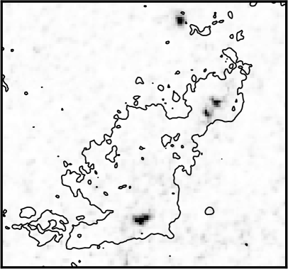
Operationally, clusters are often defined and identified as groups of stars whose stellar surface density exceeds that of field stars of the same physical type (see, e.g., Wilking & Lada, 1985; Lada et al., 1991; Carpenter, 2000). In this respect, embedded clusters pose special problems because they are buried in dust and gas, and therefore are often not even visible in optical images; moreover, their shape is often elongated and clumpy, reflecting the initial structure of the dense molecular gas (Gutermuth et al., 2005; Megeath et al., 2016). However, even with infrared observations, discovering deeply embedded clusters and measuring their basic parameters (such as surface density and size) can still be a challenge since the associated dust extinguishes both the cluster members and the field stars behind the cloud (see, e.g., Román-Zúñiga et al., 2008). In fact, typical optical or near-infrared observations stellar fields around molecular clouds show underdensities at the location of the clouds because of the effects of extinction on the density of background stars. In such a situation the observed cluster stellar surface density can be comparable or even less than the unobscured field stellar surface density (see Fig. 1).

Figure 1: A one-dimensional sketch figure that illustrates the difficulties encountered in detecting embedded clusters. The bottom black line shows the extinction profile of a molecular cloud. As a result of the extinction, background stars in the field show an underdensity. Even if an embedded cluster is present, the total observed star surface density does not reveal it, making it virtually impossible to detect the cluster without the use of the technique described in this paper.

Different authors have used different techniques to take into account the effects of extinction in the identification and characterization of star clusters. Carpenter (2000) built density maps in the direction of nearby molecular clouds using the 2MASS Point Source Catalog, and corrected the effect of dust extinction using publicly available CO maps (converted into infrared extinction with a constant X-factor). In his technique, the extinction correction is only applied to field stars: the cluster stellar density is obtained by subtracting an extinction-corrected model of the field stellar density to the observed stellar density. Moreover, the use of CO maps and the largely uncertain X-factor represent a primary source of error.

An opposite approach has been adopted by Cambrésy et al. (2013), who studied star clusters embedded in the Rosette nebula using 2MASS data. In this case, the local extinction was determined directly from the stellar near-infrared colors, and a correction for the effects of extinction was applied to each star. In practice, as noted by the authors themselves, the correction applied would only be correct for background stars, while it is used for all stars (including the foreground, which should not be corrected, and embedded ones, which should be partially corrected). Things are further complicated because molecular clouds are know to have steep gradients in their column densities, and these, if undetected (because of resolution effects, which is surely the case of the Rosette cloud at the 2MASS resolution), would introduce further biases in the extinction map and in the correction to the cluster richness.

Cambrésy et al. (2006) use yet another technique (similar to Cambrésy et al., 2002) to study the properties of IC 348 in Perseus. The basic idea is that two independent measurements of extinction in molecular clouds are available, one from the star color excess (here applied to $H-K$ color), and one from the star number counts. In absence of contaminants, both measurements should agree. The presence of a cluster, however, will affect both the color excess measurement (in a way that depends on the intrinsic color of the cluster members) and the star count method (in a way that depends on the location of the cluster within the cloud). The difference of the two extinction estimates is a proxy for the cluster density. The various assumptions made when applying this technique (in particular, the degree of embedding of the cluster within the cloud) needs to be resolved by calibrating it using independent measurements of cluster richness: this clearly limits its application.

In this paper we present a new methodology to identify and characterize clusters in wide-field or all sky, multi-band, infrared imaging surveys. The method is based on the production of extinction-corrected maps of stellar surface density, and takes advantage of the different $H$-band luminosity functions of embedded clusters with respect to that of the background population. Additionally, in contrast to the methods described above, it is able to correct for cluster members unidentified because of extinction in a way that takes into account the position of the cluster within the cloud along the line of sight. The technique is based on a rigorous mathematical framework; this provides a clear advantage, in that we can perform a detailed statistical analysis of the method. But the detailed mathematical derivation of this method might not be of as much interest to astronomers as its implementation. However, we stress that those readers not interested in the detailed mathematical aspects of the derivation can still benefit from the method proposed here, because its application is simple and straightforward: Eq(30), with optionally a second expression for the noise estimate, Eq. (31). We also provide a pseudo-code for it in the appendix.

This paper is organized as follows. In Sect. 2 we present the general framework and discuss the standard technique generally employed to identify clusters. In Sect. 3 we present our new method and we discuss its practical implementation in Sect. 4. Simple numerical tests used to validate the method are described in Sect. 5, while the results of an application to the Orion molecular complex are discussed in Sect. 6. Finally, we summarize the results obtained in this paper in Sect. 7.

2 The standard technique

Traditionally, star clusters are identified as overdensities in the distribution of stars. Although many different options are available to estimate the local angular density of stars $\sigma$ (see, e.g., von Hoerner, 1963; Casertano & Hut, 1985; Gutermuth et al., 2009), we consider in this paper the simple “moving average” estimate

$$\hat{\sigma}(\@vec{x})=\sum_{n=1}^{N}W\bigl{(}\@vec{x}-\@vec{x}_{n}\bigr{)}\;.$$ (1)

Here $n$ runs on the individual stars, $\{\@vec{x}_{n}\}$ are the locations of the various stars, and $W$ is a window function, normalized to unity:

$$\int W(\@vec{x}^{\prime})\,\mathrm{d}^{2}x^{\prime}=1\;.$$ (2)

So, by construction, $W$ has a unit of one over area. As a simple example, suppose that $W$ is taken to be a top-hat function:

$$W(\@vec{x}^{\prime})=\begin{cases}1/(\pi r^{2})&\text{if $|\@vec{x}^{\prime}|<r\;,$}\\ 0&\text{otherwise}\;.\end{cases}$$ (3)

In this case, the sum of Eq. (1) runs just over the $N_{r}$ stars within an angular distance $r$ from the point of the estimate, and the observed estimates reduces to

$$\hat{\sigma}=\frac{N_{r}}{\pi r^{2}}\;.$$ (4)

For a constant density of stars, this quantity is unbiased, in the sense that the mean (ensemble average) $E$ of $\hat{\sigma}$ is just the true density of stars:

$$\operatorname{E}[\hat{\sigma}]\equiv\langle\hat{\sigma}\rangle=\frac{\operatorname{E}[N_{r}]}{\pi r^{2}}=\sigma\;,$$ (5)

and the associated variance is

$$\operatorname{Var}[\hat{\sigma}]=\frac{\operatorname{E}[N_{r}]}{(\pi r^{2})^{2}}=\frac{\sigma}{\pi r^{2}}\;.$$ (6)

This equation shows that the error associated with the measured star density decreases as $N_{r}^{-1/2}$: therefore, if it is known that the density of stars is constant, to determine its value it is sensible to use relatively large window functions $W$.

More generally, if the star density is variable, the average measured density can be shown to be a convolution of the true density with the window function $W$:

$$\operatorname{E}[\hat{\sigma}](\@vec{x})=\int W(\@vec{x}-\@vec{x}^{\prime})\sigma(\@vec{x}^{\prime})\,\mathrm{d}^{2}x^{\prime}\;,$$ (7)

and the associated two point correlation function is

$$\operatorname{Cov} [\hat{\sigma}](\@vec{x},\@vec{x}^{\prime})$$

$${}\equiv\operatorname{E}\Bigl{[}\bigl{(}\hat{\sigma}(\@vec{x})-\operatorname{E}[\hat{\sigma}](\@vec{x})\bigr{)}\bigl{(}\hat{\sigma}(\@vec{x}^{\prime})-\operatorname{E}[\hat{\sigma}](\@vec{x}^{\prime})\bigr{)}\Bigr{]}$$

$${}=\int W(\@vec{x}-\@vec{x}^{\prime\prime})W(\@vec{x}^{\prime}-\@vec{x}^{\prime\prime})\sigma(\@vec{x}^{\prime\prime})\,\mathrm{d}^{2}x^{\prime\prime}\;.$$ (8)

Equation (7) shows that $W$ sets the scale for the resolution of the density map; similarly, Eq. (2) shows that points close enough in the density map will have correlated noise. Therefore, if one aims at finding changes in the star density (such as a star cluster), the window function should have a scale that is comparable or smaller than the typical size of the variations of the star density. However, this is in tension with the noise properties of Eq. (2), because a small window function implies a large noise.

In order to be able to detect a star cluster, the measured density of stars at the location of the cluster must differ from the average density much more than the standard deviation of $\hat{\sigma}$. Hence, the quantity $\operatorname{Cov}[\hat{\sigma}](\@vec{x},\@vec{x})$ sets the sensitivity of the cluster finding algorithm. In general the true density $\sigma=\sigma_{\mathrm{field}}+\sigma_{\mathrm{cluster}}$ is the sum of the field density and of the cluster density, and in some cases $\sigma_{\mathrm{cluster}}\ll\sigma_{\mathrm{field}}$. In these conditions the error is dominated by the shot-noise due to the field star population. In reality, many other effects can prevent the discovery and characterization of star clusters:

• Extinction by dark nebulæ, which reduces the surface density of background sources;

• The galactic structure, which induces smooth large-scale variations;

• Differences in the sensitivity across a mosaic image due to changes in the observational conditions;

• Other systematical observational effects, such halos produced by bright objects within the image;

2.1 Extinction correction

Among the effects listed above, the first one is particularly important for young clusters, since these objects tend to be deeply embedded and thus can escape a detection; additionally, detected clusters are plagued by large uncertainties in their physical properties (number of stars, mass, and size). For this reason, Cambrésy et al. (2013) developed a technique to perform a simple correction of the results produced by Eq. (1). They noted that the density of background stars observed through a molecular cloud decreases by a factor $10^{-\alpha A}$, where $\alpha$ is the exponential slope of the number counts and $A$ is the extinction, both in the band used for the observation. Therefore, to account for the undetected stars one can just multiply the local density estimate $\hat{\sigma}(\@vec{x})$ by $10^{\alpha A(\@vec{x})}$, where $A(\@vec{x})$ is the local estimate extinction (i.e., the extinction derived from an extinction map at the location of the $\@vec{x}$).

The problem of this approach is that it uses the same correction factor for foreground stars, embedded objects, and background stars, which generally results in an overestimate of the local corrected star density. Additionally, the same correction is applied to young stellar objects (YSOs) and field stars, which however have number count distributions very different. This leaves a large uncertainty on the corrected $\hat{\sigma}(\@vec{x})$ and, ultimately, on the characterization of each cluster.

3 Maximum-likelihood approach

3.1 Constant extinction, no weighting

As discussed in the previous section, the error associated to $\hat{\sigma}$ is often dominated by shot noise due to the field star population. However, as mentioned, YSOs have photometric properties that differ significantly from these of field stars: the former have a $H$-band luminosity function (hereafter HLF) that can be approximated by a Gaussian distribution (Muench et al., 2002), while the latter have a HLF that follows, up to $H\sim$18\text{\,}\mathrm{m}\mathrm{a}\mathrm{g}$$, an exponential with slope $\alpha\sim 0.33$ (see, e.g., Meingast et al., 2016). This suggests that we might use suitable cuts in the $H$-band to reduce the number of field stars, while essentially retaining all YSOs, thus gaining in terms of noise. However, this naive procedure is difficult to apply, since both YSOs and field stars are also affected by extinction, which would change the shape and the peaks of the respective HLFs. Therefore, we are forced to use a more systematic approach.

Let us first model the observed $H$-band luminosity function for a set of angularly close stars (i.e., in a patch of the sky). We suppose that the true, unextinguished HLF can be described as a mixture of $L$ different HLFs, corresponding to different stellar populations (in the situation considered later on in this paper we will use just two components, one for the field stars and one for the YSOs, but deeper observations might require the inclusion of a third component corresponding to galaxies and following exponential number counts with a slope of $0.6$; see Hubble, 1926). The observed HLF differs from the true one because of extinction and because of incompleteness in the faint end; additionally, we will also have photometric errors, but generally these will be small compared to the typical width of the various HLF components, and for the sake of simplicity are therefore neglected here. We can thus write finally the observed HLF, measured in units of stars per area per magnitude bin, as

$$\sigma(m)=c(m)\sum_{i=1}^{L}\sigma_{i}p_{i}(m-A)\;,$$ (9)

where $A$ is the $H$-band extinction, $c(m)$ is the completeness function (i.e. the probability to detect a star with apparent magnitude $m$), $p_{i}(m)$ is the probability distribution for the $i$-th component of the HLF, and $\sigma_{i}$ is a coefficient that indicates the predominance of the $i$-th component in the HLF. In order to give $\sigma_{i}$ a simple interpretation, it is useful to take $p_{i}$ suitably normalized. In particular, we assume that

$$\int c(m)p_{i}(m)\,\mathrm{d}m=1\;.$$ (10)

With this choice, $\sigma_{i}$ can be identified as the observed angular density of stars for the $i$-th component in absence of extinction.

Our goal is to infer the parameters $\{\sigma_{i}\}$ from a set of observed $H$-band magnitudes $\{m_{n}\}$ in a patch of the sky of area $S$; we will then repeat this operation in different directions in order to build maps of densities for the various components. This will allow us to identify overdensities in each component, such as in the YSO one. To this purpose, we use Eq. (9) to write the log-likelihood following the prescriptions of Lombardi et al. (2013). The entire analysis is done in the magnitude space, by using $S\sigma$ as the probability distribution density for the magnitudes:

$$\ln\mathcal{L}={} \sum_{n=1}^{N}\ln S\sigma(m_{n})-\int S\sigma(m)\,\mathrm{d}m$$

$${}={} \sum_{n=1}^{N}\biggl{[}\ln Sc(m_{n})\sum_{i=1}^{L}\sigma_{i}p_{i}(m_{n}-A)\biggr{]}$$

$${}-\int Sc(m)\sum_{i=1}^{L}\sigma_{i}p_{i}(m-A)\,\mathrm{d}m\;.$$ (11)

This likelihood can be used in Bayes’ theorem to infer a posterior probability for the densities $\{\sigma_{i}\}$. More simply, we can just find the most likely parameters $\{\sigma_{i}\}$ using a maximum likelihood approach. To this purpose, we consider

$$\frac{\partial\ln\mathcal{L}}{\partial\sigma_{i}}=\sum_{n=1}^{N}\frac{c(m_{n})p_{i}(m_{n}-A)}{\sigma(m_{n})}-S\!\int c(m)p_{i}(m-A)\,\mathrm{d}m\;.$$ (12)

The maximum likelihood solution is given by the set of densities $\sigma_{i}$ that maximize $\mathcal{L}$ or, equivalently, $\ln\mathcal{L}$, i.e. by the zero of Eq. (12); that is, we need to solve

$$\sum_{n=1}^{N}\frac{c(m_{n})p_{i}(m_{n}-A)}{\sigma(m_{n})}=S\!\int c(m)p_{i}(m-A)\,\mathrm{d}m\;.$$ (13)

Unfortunately, the solution of this equation for $L>1$ cannot be provided in analytic form, and must be obtained by numerical methods. We will discuss below in Sect. 3.3 simple ways to find it.

We can obtain an estimate of the errors associated to the measurements $\sigma_{i}$ from the Fisher information matrix (see, e.g., Feigelson & Babu, 2012), that we recall is defined as

$$I_{ij}=\operatorname{E}\left[\frac{\partial\ln\mathcal{L}}{\partial\sigma_{i}}\frac{\partial\ln\mathcal{L}}{\partial\sigma_{j}}\right]=-\operatorname{E}\left[\frac{\partial^{2}\ln\mathcal{L}}{\partial\sigma_{i}\,\partial\sigma_{j}}\right]\;.$$ (14)

The Fisher information matrix is related to the minimum covariance matrix that can be attained by an unbiased estimator, as provided by the Cramér-Rao bound:

$$\operatorname{Cov}[\sigma]\geq I^{-1}\;.$$ (15)

Since the maximum-likelihood estimator is asymptotically efficient (i.e. it attains the Cramér-Rao bound when the sample size tends to infinity) and the resulting errors on $\hat{\sigma}$ tend to a multivariate Gaussian distribution, it is interesting to obtain an analytic result for the information matrix.

The Fisher information matrix can be readily evaluated from our data using Eq. (12) of Lombardi et al. (2013):

$$I_{ij}=S\!\int\frac{c^{2}(m)p_{i}(m-A)p_{j}(m-A)}{\sigma(m)}\,\mathrm{d}m\;.$$ (16)

This relation is interesting from several points of view. First, note that the Fisher matrix contains elements outside the diagonal, unless the probability distributions for the various components do not overlap, i.e. have non-intersecting support: this would basically mean that we could immediately tell to which component belongs a star from its unextinguished magnitude. Second, note that all elements of the matrix are non-negative and therefore, in case of $L=2$ components, $\operatorname{Cov}[\sigma]\simeq I^{-1}$ will have non-positive elements off-diagonal: in other words, the measurements of the two densities $\sigma_{1}$ and $\sigma_{2}$ will be affected by a negative correlation. This is expected and corresponds to a classification error: if $p_{1}$ overlaps with $p_{2}$, we cannot uniquely associate stars to each different population and in general an overestimate of one population is done at the expenses of an underestimate of the other population.

It is instructive to consider the form of the information matrix in the special case where $L=1$. When just one component is used, then $I$ is a scalar and it reduces to

$$I=\frac{S}{\sigma}\int c(m)p(m-A)\,\mathrm{d}m=\frac{S^{2}}{\operatorname{E}[N]}\;,$$ (17)

where $\operatorname{E}[N]=S\sigma$ is the average number of stars observed in the area $S$. Its inverse, $I^{-1}$, is therefore $\operatorname{E}[N]/\sigma^{2}$, as expected from a simple Poisson statistics.

With $L\geq 2$, in principle we can encounter cases where the Fisher information matrix is singular. Given the analytic form of $I$, this happens in particular when the two components have the exact same probability distributions within the support of $c(m)$, i.e. $c(m)p_{i}(m)=c(m)p_{j}(m)$: in this case, the corresponding rows (or columns) of $I$ are identical. In such a situation, clearly, it is virtually impossible to classify objects as one of the two degenerate components, and therefore the uncertainty on the respective densities $\sigma_{i}$ and $\sigma_{j}$ are infinite.

For completeness, we also report the expected maximum value of the log-likelihood

$$\operatorname{E}[\mathcal{L}]=\frac{L}{2}+S\!\int\sigma(m)\bigl{[}\ln S\sigma(m)-1\bigr{]}\,\mathrm{d}m\;,$$ (18)

and the associated variance

$$\operatorname{Var}[\mathcal{L}]=S\!\int\sigma(m)\ln^{2}S\sigma(m)\,\mathrm{d}m\;.$$ (19)

These equations can be used to verify that the chosen model (9) can account well for the data.

3.2 Differential extinction and spatial weight

So far, we have assumed that all stars are subject to the same extinction $A$; moreover, we have not weighted stars depending on their angular position as done in Eq. (1). In this section we intend to remove these two limitations and consider the full problem.

The simpler approach to include the effects of differential extinction is to consider the joint density in magnitudes and positions. In this framework, we can rewrite Eq. (3.1) for log-likelihood as

$$\ln\mathcal{L}={} \sum_{n=0}^{N}\ln\sigma(m_{n},\@vec{x}_{n})-\int\mathrm{d}m\int\mathrm{d}^{2}x^{\prime}\,\sigma(m,\@vec{x}^{\prime})\;.$$ (20)

In this equation the quantity $\sigma(m,\@vec{x}^{\prime})$ represents the predicted density of stars with magnitude $m$ at the location $x^{\prime}$. Similarly to Eq. (9), we write this quantity as a mixture of different densities, corresponding to different stellar populations:

$$\sigma(m,\@vec{x}^{\prime})=c(m)\sum_{i=1}^{L}\sigma_{i}(\@vec{x}^{\prime})p_{i}\bigl{(}m-A(\@vec{x}^{\prime})\bigr{)}\;,$$ (21)

where $\sigma_{i}(\@vec{x}^{\prime})$ represents the density of stars of class $i$ at the sky position $\@vec{x}^{\prime}$. In order to proceed, we need to model these densities. A simple and consistent way of doing this, is to suppose that $\ln\sigma_{i}(\@vec{x}^{\prime})$ can be written as the weighted sum of two terms: one, $\ln\sigma(\@vec{x})$, associated to the density at the point of interest $\@vec{x}$ (the point where we intend to evaluate the local densities of stellar populations); and one, $\ln\tau_{i}(\@vec{x}^{\prime})$, which parametrizes the local changes of the densities. As a result, we write

$$\sigma_{i}(\@vec{x}^{\prime})=\bigl{(}\sigma_{i}(\@vec{x})\bigr{)}^{\omega(\@vec{x}-\@vec{x}^{\prime})}\bigl{(}\tau_{i}(\@vec{x}^{\prime})\bigr{)}^{1-\omega(\@vec{x}-\@vec{x}^{\prime})}\;.$$ (22)

The function $\omega$ describes the spatial correlation between densities at different positions and plays a central role in identifying which stars contribute to the density estimate at $\@vec{x}$.

We can now insert Eqs. (22) and (21) in Eq. (20) and find the maximum likelihood solution over $\sigma_{i}(\@vec{x})$. Calling $A_{n}\equiv A(\@vec{x}_{n})$ the extinction suffered by the $n$-th star, we find

$$\frac{\partial\ln\mathcal{L}}{\partial\sigma_{i}(\@vec{x})}=\sum_{n=1}^{N}\omega(\@vec{x}-\@vec{x}_{n})\frac{p_{i}(m_{n}-A_{n})\sigma_{i}(\@vec{x}_{n})/\sigma_{i}(\@vec{x})}{\sum_{j}\sigma_{j}(\@vec{x}_{n})p_{j}(m_{n}-A_{n})}$$

$$\quad-\int\mathrm{d}m\,c(m)\int\mathrm{d}^{2}x^{\prime}\,\omega(\@vec{x}^{\prime})p_{i}\bigl{(}m-A(\@vec{x}^{\prime})\bigr{)}\sigma_{i}(\@vec{x}^{\prime})/\sigma_{i}(\@vec{x})\;.$$ (23)

We now make an important assumption. Because of the form of the parametrization (22), a solution for the maximum likelihood can only be found if we specify the functional form of the functions $\tau_{i}(\@vec{x}^{\prime})$. However, these functions are truly unknown, since they parametrize the local changes of the various densities, which in turn depend on the local density map. Using a statistical approach, however, it is natural to assume that these functions have the same distribution of $\sigma_{i}(\@vec{x})$, the quantity we are interested in. As a result, if we take an average of Eq. (3.2), terms such as $\sigma_{i}(\@vec{x}^{\prime})/\sigma_{i}(\@vec{x})$ cancel out:

$$\frac{\partial\ln\mathcal{L}}{\partial\sigma_{i}(\@vec{x})}=\sum_{n=1}^{N}\omega(\@vec{x}-\@vec{x}_{n})\frac{p_{i}(m_{n}-A_{n})}{\sum_{j}\sigma_{j}(\@vec{x})p_{j}(m_{n}-A_{n})}$$

$$\quad-\int\mathrm{d}m\,c(m)\int\mathrm{d}^{2}x^{\prime}\,\omega(\@vec{x}^{\prime})p_{i}\bigl{(}m-A(\@vec{x}^{\prime})\bigr{)}\;.$$ (24)

Before proceeding, it is useful to consider the solution of the maximum likelihood approach in the simple case where there is a single population of stars and where the extinction vanishes, $A(\@vec{x}^{\prime})=0$. We find in this case

$$\frac{\partial\ln\mathcal{L}}{\partial\sigma(\@vec{x})}=\sum_{n=1}^{N}\frac{\omega(\@vec{x}-\@vec{x}_{n})}{\sigma(\@vec{x})}-\int\mathrm{d}^{2}x^{\prime}\,\omega(\@vec{x}^{\prime})\;,$$ (25)

where we have used the normalization property (10). The solution of this equation is immediately found as

$$\sigma(\@vec{x})=\sum_{n=1}^{N}W(\@vec{x}-\@vec{x}_{n})\;,$$ (26)

where

$$W(\@vec{x})=\frac{\omega(\@vec{x})}{\int\omega(\@vec{x}^{\prime})\,\mathrm{d}^{2}x^{\prime}}$$ (27)

We have therefore recovered Eq. (1), with the correct normalization (2) for the weight $W$.

In the general case, the maximum-likelihood solution of Eq. (3.2) must be obtained numerically. The errors associated to the solutions can be estimated using the Fisher matrix. In our case, we can obtain the Fisher matrix from

$$I_{ij}(\@vec{x})={} \iint\mathrm{d}m\,\mathrm{d}^{2}x^{\prime}\,\frac{1}{\sigma(m,\@vec{x}^{\prime})}\frac{\partial\sigma(m,\@vec{x}^{\prime})}{\partial\sigma_{i}(\@vec{x})}\frac{\partial\sigma(m,\@vec{x}^{\prime})}{\partial\sigma_{j}(\@vec{x})}$$

$${}={} \iint\mathrm{d}m\,\mathrm{d}^{2}x^{\prime}\,c^{2}(m)\omega^{2}(\@vec{x}-\@vec{x}^{\prime})\times$$

$$\qquad\frac{p_{i}\bigl{(}m-A(\@vec{x}^{\prime})\bigr{)}p_{j}\bigl{(}m-A(\@vec{x}^{\prime})\bigr{)}}{\sigma(m,\@vec{x}^{\prime})}\frac{\sigma_{i}(\@vec{x}^{\prime})\sigma_{j}(\@vec{x}^{\prime})}{\sigma_{i}(\@vec{x})\sigma_{j}(\@vec{x})}\;.$$ (28)

As before, we can replace $\@vec{x}$ to $\@vec{x}^{\prime}$ in all arguments of $\sigma_{i}$, with the justification that the statistical properties of $\sigma$ are invariant upon translation. We will discuss in the next section useful expressions to evaluate this quantity in practical cases.

Function	Support	$\omega(\@vec{x})$	$W(\@vec{x})$	Eff. area
Top-hat	$\@vec{|}\@vec{x}|\leq s$	$1$	$1/(\pi s^{2})$	$\pi s^{2}$
Conic	$\@vec{|}\@vec{x}|\leq s$	$2(1-|\@vec{x}|/s)$	$3(1-|\@vec{x}|/s)/(\pi s^{2})$	$2\pi s^{2}/3$
Parabolic	$\@vec{|}\@vec{x}|\leq s$	$3(1-|\@vec{x}|^{2}/s^{2})/2$	$2(1-|\@vec{x}|^{2}/s^{2})/(\pi s^{2})$	$3\pi s^{2}/4$
Gaussian	$\mathbb{R}^{2}$	2 $\exp\bigl{(}-|\@vec{x}|^{2}/2s^{2}\bigr{)}$	$\exp\bigl{(}-|\@vec{x}|^{2}/2s^{2}\bigr{)}/(2\pi s^{2})$	$4\pi s^{2}$

Table 1: Different two-dimensional spatial functions $\omega(\@vec{x})$ and corresponding weight functions $W(\@vec{x})$. All functions considered here are axisymmetric and include a spatial scale $s$.

3.3 Implementation

The algorithm proposed in this paper is essentially the search of the solutions of Eq. (3.2) as a function of the star densities $\{\sigma_{i}\}$ corresponding to the various components or star populations. The same procedure must be applied to different patches of the sky, so that maps of the star densities can be obtained. These, in turn, will allow us to identify and characterize star clusters, and in particular embedded ones.

Although the practical implementation of the algorithm follows this schema, a number of technical and theoretical aspects must be correctly addressed in order to optimize the detection and make the technique efficient.

First, we note that a simple way to obtain the (positive) solutions of Eq. (3.2) is through the use of a recursive formula. To this purpose, multiply both members of this equation by $\sigma_{i}(\@vec{x})$, and solve for this quantity, thus obtaining the expression

$$\sigma_{i}(\@vec{x})\leftarrow\frac{\displaystyle\sum_{n=1}^{N}\omega(\@vec{x}-\@vec{x}_{n})\frac{\sigma_{i}(\@vec{x})p_{i}(m_{n}-A_{n})}{\sum_{j=1}^{L}\sigma_{j}(\@vec{x})p_{j}(m_{n}-A_{n})}}{\displaystyle\int\mathrm{d}m\,c(m)\int\mathrm{d}^{2}x^{\prime}\,\omega(\@vec{x}^{\prime})p_{i}\bigl{(}m-A(\@vec{x}^{\prime})\bigr{)}}\;.$$ (29)

Unfortunately, we are unable to use this equation because we only know the extinction at the locations of the stars $A_{n}\equiv A(\@vec{x}_{n})$: this prevents us from evaluating the integral over $\mathrm{d}x^{2}$ in the denominator. We can, however, move the denominator inside the sum, and evaluate the second integral by replacing $A(\@vec{x})$ with $A(\@vec{x}_{n})$, the extinction at the direction of each star. Additionally, using the same argument that has been employed in Eq. (3.2), that is the similarity between $\sigma$ and $\tau$, it is convenient to replace $\sigma_{i}(\@vec{x})$ with $\sigma_{i}(\@vec{x}_{n})$ in the numerator. This procedure leads to the iteration

$$\sigma_{i}(\@vec{x})\leftarrow\sum_{n=1}^{N}\frac{\displaystyle W(\@vec{x}-\@vec{x}_{n})\frac{\sigma_{i}(\@vec{x}_{n})p_{i}(m_{n}-A_{n})}{\sum_{j=1}^{L}\sigma_{j}(\@vec{x}_{n})p_{j}(m_{n}-A_{n})}}{\int\mathrm{d}m\,c(m)p_{i}(m-A_{n})}\;.$$ (30)

Equation (30) is the solution proposed in this paper to estimate the local density of stars. As indicated by the left arrow symbol, we can obtain the set of values $\{\sigma_{i}\}$ by starting with some arbitrary (positive) values for these quantities, and then by calculating updated values of $\sigma_{i}$ by applying Eq. (30). The convergence is usually reached within a few tens of iterations.

Note that Eq. (30) has a simple interpretation. Let us ignore for a moment the weight $W$, i.e. let us assume that all stars have the same weight. The sum in Eq. (30) is carried out over all stars in the patch of the sky, but each star is counted only partially (i.e., contributes with a term between zero and unity in the sum): precisely, each star contributes by the computed probability that the star be associated with the $i$-th component. The way this probability is computed is actually a simple application of Bayes’ theorem, where $p_{i}(m_{n}-A_{n})$ plays the role of the likelihood, $\sigma_{i}(\@vec{x}_{n})$ is proportional to the prior that the star is of class $i$, and the sum over $j$ in the denominator is proportional to the evidence. The result of the sum of these terms is divided by the by the result of the integral: this is a correcting factor that takes into account the fact that, because of extinction and incompleteness, we will miss a fraction of stars. Note also that Eq. (30) can be also considered as a special case of a $K$-means soft clustering algorithm where the only unknown quantities are the classes $\sigma_{i}$ (see MacKay, 2003).

Before proceeding, it is useful to recall the hypotheses of this algorithm and its strengths. First, we assume that we have some knowledge of the $H$-band luminosity function for the various populations of stars that are likely to be present in the field. In practice, we will generally use two probabilities, one for the field stars, and one for the YSOs. Second, we assume that we have measured the extinction $A_{n}$ of each star: note that this is not the average extinction at the location of the star, which might be very different because of perspective effects: for example, a foreground star in front of a cloud would have $A_{n}\simeq 0$, while the average extinction would be significant. This way, the algorithm can directly account for foreground contamination: foreground stars will not be corrected in their counts, since the integral in the denominator of Eq. (30) will evaluate to unity. Similarly, stars within molecular clouds will be corrected only for the amount of material that is really in front of them.

Finally, we stress that the iterative procedure proposed here only find positive solutions for the values $\sigma_{i}$. Although reasonable, nevertheless this choice inevitably introduces biases in the results: for example, in a region where no YSO is present, because of errors we will still measure small positive values for the density of YSOs. However, numerical tests have shown that the bias amount is limited; moreover, a reduction of the bias is associated to a large increase in the scatter. Therefore, we will force the $\sigma_{i}$ to be positive and use Eq. (30) for the solution.

The uncertainties associated to Eq. (30) can be computed from the Fisher matrix. For practical applications, it is convenient to rewrite Eq. (3.2) by replacing the integrals over $\mathrm{d}m$ and $\mathrm{d}^{2}x^{\prime}$ with a sum over the observed objects. This leads to the approximated Fisher matrix expression

$$I_{ij}=\sum_{n=1}^{N}\frac{\omega^{2}(\@vec{x}-\@vec{x}_{n})c^{2}(m_{n})p_{i}(m_{n}-A_{n})p_{j}(m_{n}-A_{n})}{\sigma^{2}(m_{n},\@vec{x}_{n})}\;.$$ (31)

In this equation, we take the spatial function $\omega$ to be normalized such that

$$\int\omega(\@vec{x}^{\prime})\,\mathrm{d}^{2}x^{\prime}=\int\omega^{2}(\@vec{x}^{\prime})\,\mathrm{d}^{2}x^{\prime}\;;$$ (32)

that is, in terms of $W$,

$$\omega(\@vec{x})=\frac{W(\@vec{x})}{\int W^{2}(\@vec{x}^{\prime})\,\mathrm{d}^{2}x^{\prime}}\;.$$ (33)

Table 1 reports a few common choices for the spatial function $\omega(\@vec{x})$ and the corresponding weight function $W(\@vec{x})$, both correctly normalized. As usual, the covariance matrix associated with the measurements of the densities $\sigma_{i}$ can be computed from the inverse of the Fisher matrix, $I^{-1}$.

4 Simulations

$\sigma_{1}$	$\sigma_{2}$	$\langle(I^{-1})_{11}\rangle$	$\langle(I^{-1})_{12}\rangle$	$\langle(I^{-1})_{22}\rangle$
$\langle\hat{\sigma}_{1}\rangle$	$\langle\hat{\sigma}_{2}\rangle$	$\operatorname{Var}[\sigma_{1}]$	$\operatorname{Cov}[\sigma_{1},\sigma_{2}]$	$\operatorname{Var}[\sigma_{2}]$
$5.00$	$20.00$	$33.38$	$-19.13$	$35.27$
$5.30$	$19.87$	$21.37$	$-12.09$	$29.60$
$20.00$	$5.00$	$47.44$	$-19.02$	$22.34$
$19.79$	$5.21$	$43.31$	$-13.83$	$16.33$
$10.00$	$10.00$	$47.44$	$-19.02$	$22.34$
$10.05$	$9.95$	$30.63$	$-13.97$	$21.04$

Table 2: Summaries of the results of simulations.

Figure 2: The distributions of measured densities in a simulation with $\sigma_{1}=5$ and $\sigma_{2}=20$ (histogram), together with the predicted Gaussian distribution obtained according to the Fisher matrix evaluated from Eq. (31). The excess of small values of $\hat{\sigma}_{1}$ is due to the constraint that $\hat{\sigma}\geq 0$ imposed by the algorithm.

Figure 3: The distribution of measured total density $\hat{\sigma}_{1}+\hat{\sigma}_{2}$ in a simulation with $\sigma_{1}=5$ and $\sigma_{2}=20$, together with the predicted Gaussian distribution (derived from the Fisher matrix). The distribution is essentially unbiased; moreover, because of the anticorrelation between $\hat{\sigma}_{1}$ and $\hat{\sigma}_{2}$, the total density has significantly less scatter than both $\hat{\sigma}_{1}$ and $\hat{\sigma}_{2}$.

Figure 4: The distributions of measured densities in a simulation with $\sigma_{1}=20$ and $\sigma_{2}=5$.

Figure 5: The distributions of measured densities in a simulation with $\sigma_{1}=10$ and $\sigma_{2}=10$.

Figure 6: The biases in the measured densities for $\sigma_{1}=10$ and $\sigma_{2}\in[0,20]$. Note how the bias essentially vanishes for $\sigma_{2}>5$.

Figure 7: The scatter on $\hat{\sigma}_{1}$ and $\hat{\sigma}_{2}$ for $\sigma_{1}=10$ and $\sigma_{2}\in[0,20]$ (dots), together with the predictions obtained from Eq. (31) (lines).

Figure 8: Violin plot showing the distribution of measured densities $\hat{\sigma}_{1}$ for $\sigma_{1}=10$ and $\sigma_{2}\in[0,20]$. Each elongated structure corresponds to a different value of $\sigma_{2}$; its width is proportional to the distribution of measured values of $\hat{\sigma}_{1}$, i.e. effectively it is a histogram displayed vertically. The small red dashes indicate the average values.

Figure 9: Violin plot showing the distribution of measured densities $\hat{\sigma}_{2}$ for $\sigma_{1}=10$ and $\sigma_{2}\in[0,20]$. The small blue dashes indicate the average values.

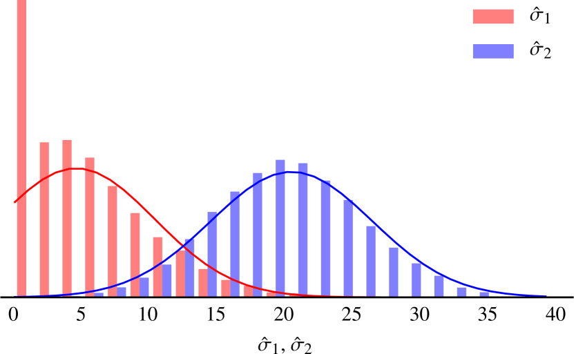
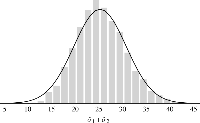
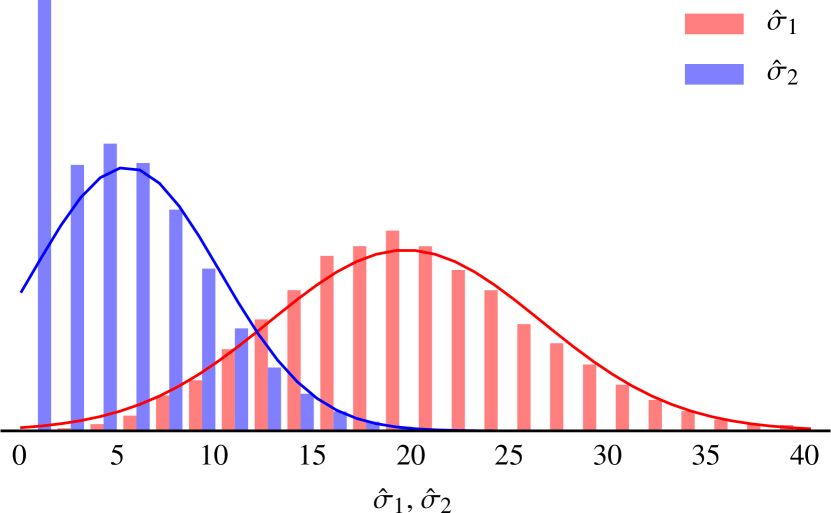
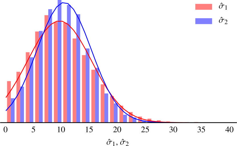
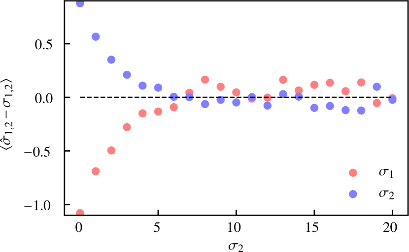
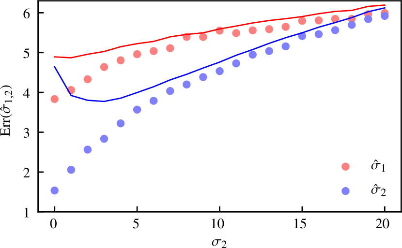
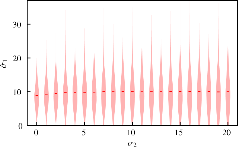
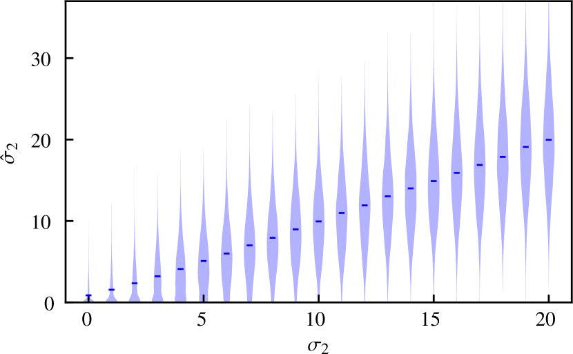
In order to test our method and verify its robustness we have performed a set of simulations. We have considered a small patch of the sky with two different stellar populations: field stars, with exponentially increasing number counts $p_{1}(m)\propto 10^{\alpha m}$, with $\alpha=$0.33\text{\,}\mathrm{m}\mathrm{a}\mathrm{g}^{-1}$$; and YSOs, with Gaussian number counts $p_{2}(m)\propto\exp\bigl{(}-(m-m_{0})^{2}/2s^{2}\bigr{)}$, with $m_{0}=$12\text{\,}\mathrm{m}\mathrm{a}\mathrm{g}$$ and $s=$1.65\text{\,}\mathrm{m}\mathrm{a}\mathrm{g}$$. We have distributed both populations randomly in the small patch of the sky considered and we have added to each star a random extinction drawn from the probability distribution $p_{A}(A)\propto A^{-2}$, in the range $A\in[0.1,2.0]\,$\mathrm{m}\mathrm{a}\mathrm{g}$$. This choice is meant to simulate the effects of differential extinction for objects within molecular clouds. Finally, we have imagined that our observations are complete up to $15\text{\,}\mathrm{m}\mathrm{a}\mathrm{g}$, and that no stars can be observed beyond that magnitude: in other words, we have modeled the completeness function as a Heaviside function $c(m)=H(15-m)$. This way, our final catalog contains, for each star, the angular position in the sky, the $H$-band magnitude, and the measured extinction. Note that the parameters used here are chosen to simulate a real situation corresponding to the sample application of Sect. 5, that is the Orion molecular cloud complex observed with 2MASS.

We have used these data in our algorithm, represented by Eqs. (30) and (31). As weight function $W(\@vec{x})$ we have used a Gaussian, and we have chosen the angular units so that

$$\int W^{2}(\@vec{x}^{\prime})\,\mathrm{d}^{2}x^{\prime}=\left[\int W(\@vec{x}^{\prime})\,\mathrm{d}^{2}x^{\prime}\right]^{2}\;.$$ (34)

This choice guarantees that the effective area of the weight function is unity, i.e. the effective number of stars used for the analysis, in absence of extinction, would be just $\sigma_{1}+\sigma_{2}$. In reality, the presence of the extinction reduces this number by a factor that depends on the relative ratio between $\sigma_{1}$ and $\sigma_{2}$ (typically, by $\sim 20\%$).

We have then performed different simulations, with various choices for $\sigma_{1}$ and $\sigma_{2}$, to verify the ability of the algorithm to recover the input densities. Figures 2–5 show the observed distributions of $\hat{\sigma}_{1}$ and $\hat{\sigma}_{2}$, together with the predicted ones (Gaussian distributions centered on the true values of $\sigma_{1}$ and $\sigma_{2}$, with the variances predicted from the Fisher matrix $I$). In general, we can note a few points:

• When one of the input densities is below $\sim 7$, there is a clear excess of the corresponding quantity for small measured values. This is a consequence of the fact that the proposed algorithm only returns positive values for the densities.

• Except for the point above, the predicted distributions reproduce very well the measured data. The agreement is particularly good when the input densities are large.

• Overall, the total density $\sigma_{1}+\sigma_{2}$ is better constrained than the individual densities $\sigma_{1,2}$.

Figures 6 and 7 show the biases and the errors on the measured densities $\hat{\sigma}_{1,2}$ for $\sigma_{1}=10$ and $\sigma_{2}$ varying in the interval $[0,20]$. We can see that there is a measurable bias for $\sigma_{2}<5$, while the results are essentially unbiased above this value. Correspondingly, we observe in the same range $\sigma_{2}\in[0,5]$ a measured scatter in measured densities that is significantly smaller than what predicted from the Fisher matrix. For larger values of the input density the error estimate gets closer to the measured errors, but still remains slightly above. This is actually good, because implies a small overestimate of the error which will make the entire method more robust for cluster detections (that is, it will decrease the number of false positive). In summary, all these simulations confirm that the method works and that the error estimate is quite accurate.

5 Sample application: Orion

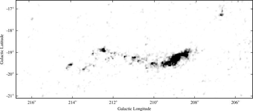
fig:30b2offfig:30b2off0fig:30b2onfig:30b2on1fig:30b3offfig:30b3off0fig:30b3onfig:30b3on1fig:30b4offfig:30b4off0fig:30b4onfig:30b4on1fig:30b5offfig:30b5off0fig:30b5onfig:30b5on1fig:30b6offfig:30b6off0fig:30b6onfig:30b6on1

Figure 10: The results of the cluster finding algorithm in Orion A using the 2MASS Point Source Catalog. The red contours shows all surface density detections $3\sigma$ above the background, while the black contour corresponds to $A_{K}=$0.3\text{\,}\mathrm{m}\mathrm{a}\mathrm{g}$$. When displayed in Adobe Acrobat, it is possible to hide the user /Subtype /Link /Border [0 0 0]/A ¡¡ /S/JavaScript /JS ( var aOCGs = this.getOCGs(), Layer; var Layers = ”fig:30b2on,fig:30b2off”.split(”,”), Active = -1, i, l; for (l=0; l¡Layers.length; l++) Layer = Layers[l]; for (i=0; aOCGs & i¡aOCGs.length; i++) if (aOCGs[i].state aOCGs[i].name == Layer) Active = l; aOCGs[i].state = false; if (Active ¿= 0) break; if (Active == -1) for (l=0; l¡Layers.length; l++) if (Layers[l] == ””) Active = l; Active = Active + 1; if (Active == Layers.length) Active = 0; Layer = Layers[Active]; for (i=0; aOCGs & i¡aOCGs.length; i++) if (aOCGs[i].name == Layer) aOCGs[i].state = true; ) ¿¿ Grid lines, the black user /Subtype /Link /Border [0 0 0]/A ¡¡ /S/JavaScript /JS ( var aOCGs = this.getOCGs(), Layer; var Layers = ”fig:30b3on,fig:30b3off”.split(”,”), Active = -1, i, l; for (l=0; l¡Layers.length; l++) Layer = Layers[l]; for (i=0; aOCGs & i¡aOCGs.length; i++) if (aOCGs[i].state aOCGs[i].name == Layer) Active = l; aOCGs[i].state = false; if (Active ¿= 0) break; if (Active == -1) for (l=0; l¡Layers.length; l++) if (Layers[l] == ””) Active = l; Active = Active + 1; if (Active == Layers.length) Active = 0; Layer = Layers[Active]; for (i=0; aOCGs & i¡aOCGs.length; i++) if (aOCGs[i].name == Layer) aOCGs[i].state = true; ) ¿¿ Extinction contours, the red contours corresponding to the user /Subtype /Link /Border [0 0 0]/A ¡¡ /S/JavaScript /JS ( var aOCGs = this.getOCGs(), Layer; var Layers = ”fig:30b4on,fig:30b4off”.split(”,”), Active = -1, i, l; for (l=0; l¡Layers.length; l++) Layer = Layers[l]; for (i=0; aOCGs & i¡aOCGs.length; i++) if (aOCGs[i].state aOCGs[i].name == Layer) Active = l; aOCGs[i].state = false; if (Active ¿= 0) break; if (Active == -1) for (l=0; l¡Layers.length; l++) if (Layers[l] == ””) Active = l; Active = Active + 1; if (Active == Layers.length) Active = 0; Layer = Layers[Active]; for (i=0; aOCGs & i¡aOCGs.length; i++) if (aOCGs[i].name == Layer) aOCGs[i].state = true; ) ¿¿ Clusters, the red dots representing the user /Subtype /Link /Border [0 0 0]/A ¡¡ /S/JavaScript /JS ( var aOCGs = this.getOCGs(), Layer; var Layers = ”fig:30b5on,fig:30b5off”.split(”,”), Active = -1, i, l; for (l=0; l¡Layers.length; l++) Layer = Layers[l]; for (i=0; aOCGs & i¡aOCGs.length; i++) if (aOCGs[i].state aOCGs[i].name == Layer) Active = l; aOCGs[i].state = false; if (Active ¿= 0) break; if (Active == -1) for (l=0; l¡Layers.length; l++) if (Layers[l] == ””) Active = l; Active = Active + 1; if (Active == Layers.length) Active = 0; Layer = Layers[Active]; for (i=0; aOCGs & i¡aOCGs.length; i++) if (aOCGs[i].name == Layer) aOCGs[i].state = true; ) ¿¿ Megeath et al. YSOs’, and the clusters’ user /Subtype /Link /Border [0 0 0]/A ¡¡ /S/JavaScript /JS ( var aOCGs = this.getOCGs(), Layer; var Layers = ”fig:30b6on,fig:30b6off”.split(”,”), Active = -1, i, l; for (l=0; l¡Layers.length; l++) Layer = Layers[l]; for (i=0; aOCGs & i¡aOCGs.length; i++) if (aOCGs[i].state aOCGs[i].name == Layer) Active = l; aOCGs[i].state = false; if (Active ¿= 0) break; if (Active == -1) for (l=0; l¡Layers.length; l++) if (Layers[l] == ””) Active = l; Active = Active + 1; if (Active == Layers.length) Active = 0; Layer = Layers[Active]; for (i=0; aOCGs & i¡aOCGs.length; i++) if (aOCGs[i].name == Layer) aOCGs[i].state = true; ) ¿¿ Names.

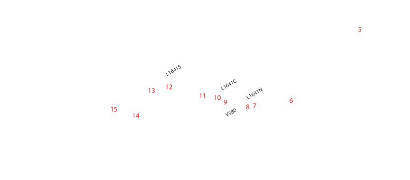
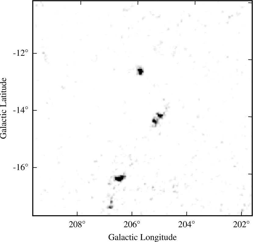
fig:30c2offfig:30c2off0fig:30c2onfig:30c2on1fig:30c3offfig:30c3off0fig:30c3onfig:30c3on1fig:30c4offfig:30c4off0fig:30c4onfig:30c4on1fig:30c5offfig:30c5off0fig:30c5onfig:30c5on1fig:30c6offfig:30c6off0fig:30c6onfig:30c6on1

Figure 11: The results of the cluster finding algorithm in Orion B using the 2MASS Point Source Catalog (see caption of Fig. 10 for the legend). Note that NGC 2023 is below the detection threshold and appears only as a weak smudge in this image. When displayed in Adobe Acrobat, it is possible to hide the user /Subtype /Link /Border [0 0 0]/A ¡¡ /S/JavaScript /JS ( var aOCGs = this.getOCGs(), Layer; var Layers = ”fig:30c2on,fig:30c2off”.split(”,”), Active = -1, i, l; for (l=0; l¡Layers.length; l++) Layer = Layers[l]; for (i=0; aOCGs & i¡aOCGs.length; i++) if (aOCGs[i].state aOCGs[i].name == Layer) Active = l; aOCGs[i].state = false; if (Active ¿= 0) break; if (Active == -1) for (l=0; l¡Layers.length; l++) if (Layers[l] == ””) Active = l; Active = Active + 1; if (Active == Layers.length) Active = 0; Layer = Layers[Active]; for (i=0; aOCGs & i¡aOCGs.length; i++) if (aOCGs[i].name == Layer) aOCGs[i].state = true; ) ¿¿ Grid, the user /Subtype /Link /Border [0 0 0]/A ¡¡ /S/JavaScript /JS ( var aOCGs = this.getOCGs(), Layer; var Layers = ”fig:30c3on,fig:30c3off”.split(”,”), Active = -1, i, l; for (l=0; l¡Layers.length; l++) Layer = Layers[l]; for (i=0; aOCGs & i¡aOCGs.length; i++) if (aOCGs[i].state aOCGs[i].name == Layer) Active = l; aOCGs[i].state = false; if (Active ¿= 0) break; if (Active == -1) for (l=0; l¡Layers.length; l++) if (Layers[l] == ””) Active = l; Active = Active + 1; if (Active == Layers.length) Active = 0; Layer = Layers[Active]; for (i=0; aOCGs & i¡aOCGs.length; i++) if (aOCGs[i].name == Layer) aOCGs[i].state = true; ) ¿¿ Extinction, the user /Subtype /Link /Border [0 0 0]/A ¡¡ /S/JavaScript /JS ( var aOCGs = this.getOCGs(), Layer; var Layers = ”fig:30c4on,fig:30c4off”.split(”,”), Active = -1, i, l; for (l=0; l¡Layers.length; l++) Layer = Layers[l]; for (i=0; aOCGs & i¡aOCGs.length; i++) if (aOCGs[i].state aOCGs[i].name == Layer) Active = l; aOCGs[i].state = false; if (Active ¿= 0) break; if (Active == -1) for (l=0; l¡Layers.length; l++) if (Layers[l] == ””) Active = l; Active = Active + 1; if (Active == Layers.length) Active = 0; Layer = Layers[Active]; for (i=0; aOCGs & i¡aOCGs.length; i++) if (aOCGs[i].name == Layer) aOCGs[i].state = true; ) ¿¿ Clusters, the red dots representing the user /Subtype /Link /Border [0 0 0]/A ¡¡ /S/JavaScript /JS ( var aOCGs = this.getOCGs(), Layer; var Layers = ”fig:30b5on,fig:30b5off”.split(”,”), Active = -1, i, l; for (l=0; l¡Layers.length; l++) Layer = Layers[l]; for (i=0; aOCGs & i¡aOCGs.length; i++) if (aOCGs[i].state aOCGs[i].name == Layer) Active = l; aOCGs[i].state = false; if (Active ¿= 0) break; if (Active == -1) for (l=0; l¡Layers.length; l++) if (Layers[l] == ””) Active = l; Active = Active + 1; if (Active == Layers.length) Active = 0; Layer = Layers[Active]; for (i=0; aOCGs & i¡aOCGs.length; i++) if (aOCGs[i].name == Layer) aOCGs[i].state = true; ) ¿¿ Megeath et al. YSOs’, or the user /Subtype /Link /Border [0 0 0]/A ¡¡ /S/JavaScript /JS ( var aOCGs = this.getOCGs(), Layer; var Layers = ”fig:30c6on,fig:30c6off”.split(”,”), Active = -1, i, l; for (l=0; l¡Layers.length; l++) Layer = Layers[l]; for (i=0; aOCGs & i¡aOCGs.length; i++) if (aOCGs[i].state aOCGs[i].name == Layer) Active = l; aOCGs[i].state = false; if (Active ¿= 0) break; if (Active == -1) for (l=0; l¡Layers.length; l++) if (Layers[l] == ””) Active = l; Active = Active + 1; if (Active == Layers.length) Active = 0; Layer = Layers[Active]; for (i=0; aOCGs & i¡aOCGs.length; i++) if (aOCGs[i].name == Layer) aOCGs[i].state = true; ) ¿¿ Names.

Figure 12: A Gaussian-kernel smoothed density map of the Megeath et al. (2016) YSO list in Orion A (top) to compare with our density map (bottom).

Figure 13: A Gaussian-kernel smoothed density map of the Megeath et al. (2016) YSO list in Orion B (left) to compare with our density map (right).

Figure 14: The distribution of $P_{\mathrm{YSO}}$, the probability that our algorithm assigns to each star to be a YSO, for the Megeath et al. (2016) YSO candidates and for all other objects in the 2MASS point source catalog.

Table 3: The YSO clusters identified in Orion A and B.

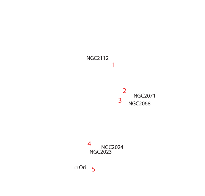
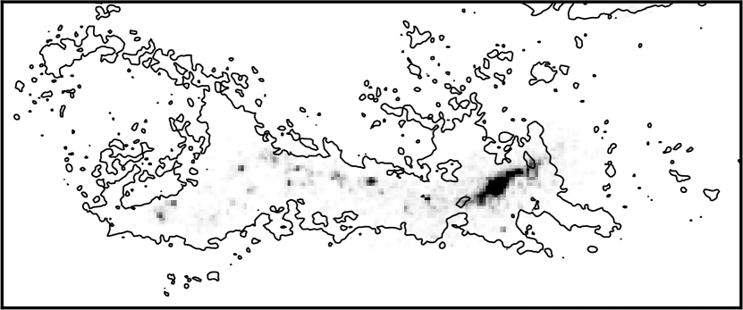
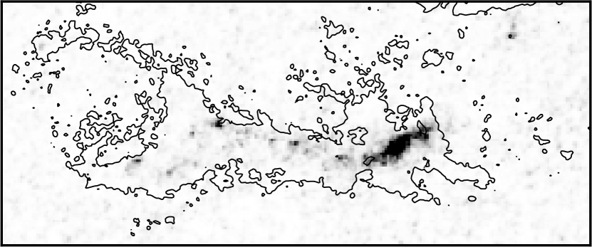
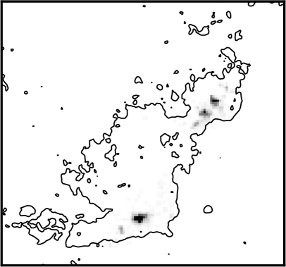
ID	$\ell$	$b$	R.A.	Dec.	Stars	$R$	$A_{K}$	Cloud	Simbad	Type
	∘	∘	∘	∘		′	$\mathrm{mag}$
1	$205.8569$	$-12.6041$	$88.4398$	$+00.4283$	$\phantom{0}\phantom{0}88\pm 14\phantom{0}$	$\phantom{0}5.2$	$0.2$	Ori B	NGC 2112	OpC
2	$205.1234$	$-14.1127$	$86.7727$	$+00.3486$	$\phantom{0}\phantom{0}78\pm 13\phantom{0}$	$\phantom{0}4.9$	$1.6$	Ori B	NGC 2071	RNe
3	$205.2984$	$-14.3236$	$86.6667$	$+00.0995$	$\phantom{0}\phantom{0}56\pm 11\phantom{0}$	$\phantom{0}4.1$	$1.4$	Ori B	M 78	RNe
4	$206.4996$	$-16.3341$	$85.4332$	$-01.8659$	$\phantom{0}188\pm 23\phantom{0}$	$\phantom{0}7.1$	$2.1$	Ori B	NGC 2024	Cl*
5	$206.8020$	$-17.3464$	$84.6710$	$-02.5928$	$\phantom{0}\phantom{0}15\pm 4\phantom{0}\phantom{0}$	$\phantom{0}2.5$	$0.1$	Ori A	sig Ori	MGr
6	$208.9681$	$-19.3846$	$83.7998$	$-05.3541$	$1601\pm 49\phantom{0}$	$19.8$	$1.1$	Ori A	M 42	HII
7	$209.9598$	$-19.6021$	$84.0276$	$-06.2867$	$\phantom{0}\phantom{0}\phantom{0}8\pm 3\phantom{0}\phantom{0}$	$\phantom{0}1.9$	$0.6$	Ori A	—	—
8	$210.1018$	$-19.6036$	$84.0865$	$-06.4071$	$\phantom{0}\phantom{0}27\pm 6\phantom{0}\phantom{0}$	$\phantom{0}3.1$	$1.1$	Ori A	LDN 1641N	Cl*
9	$210.7790$	$-19.4832$	$84.4813$	$-06.9247$	$\phantom{0}\phantom{0}\phantom{0}5\pm 3\phantom{0}\phantom{0}$	$\phantom{0}1.5$	$0.6$	Ori A	[BDB2003] G210.80-19.50	Cl*
10	$210.9941$	$-19.3347$	$84.7061$	$-07.0406$	$\phantom{0}\phantom{0}35\pm 9\phantom{0}\phantom{0}$	$\phantom{0}3.6$	$1.7$	Ori A	LDN 1641C	Cl*
11	$211.4326$	$-19.2912$	$84.9301$	$-07.3924$	$\phantom{0}\phantom{0}12\pm 5\phantom{0}\phantom{0}$	$\phantom{0}2.1$	$2.2$	Ori A	—	—
12	$212.4806$	$-18.9864$	$85.6458$	$-08.1475$	$\phantom{0}\phantom{0}91\pm 13\phantom{0}$	$\phantom{0}5.3$	$0.6$	Ori A	2MASS J05422695-0809173	Y*O
13	$212.9849$	$-19.1519$	$85.7057$	$-08.6486$	$\phantom{0}\phantom{0}\phantom{0}4\pm 2\phantom{0}\phantom{0}$	$\phantom{0}1.2$	$1.4$	Ori A	[BDB2003] G212.98-19.15	Cl*
14	$213.4450$	$-19.8466$	$85.2625$	$-09.3407$	$\phantom{0}\phantom{0}10\pm 4\phantom{0}\phantom{0}$	$\phantom{0}2.1$	$0.6$	Ori A	—	—
15	$214.0756$	$-19.6278$	$85.7219$	$-09.7820$	$\phantom{0}\phantom{0}32\pm 8\phantom{0}\phantom{0}$	$\phantom{0}3.4$	$1.1$	Ori A	[BDB2003] G214.06-19.62	Cl*

Table 4: Correspondence between the clusters identified in this work, marked with the subscript 1, and the ones identified from a smoothed version of the YSO catalog Megeath et al. (2016).

$\ell$	$b$	Stars1	Stars2	$R$	Cloud
∘	∘			′
$214.0472$	$-19.6402$	$\phantom{0}\phantom{0}12\pm 4\phantom{0}\phantom{0}$	$\phantom{0}8.9$	$\phantom{0}1.9$	Ori A
$212.9892$	$-19.1435$	$\phantom{0}\phantom{0}10\pm 5\phantom{0}\phantom{0}$	$11.5$	$\phantom{0}2.1$	Ori A
$212.4676$	$-19.0192$	$\phantom{0}\phantom{0}\phantom{0}8\pm 3\phantom{0}\phantom{0}$	$\phantom{0}3.4$	$\phantom{0}1.2$	Ori A
$210.9717$	$-19.3367$	$\phantom{0}\phantom{0}28\pm 8\phantom{0}\phantom{0}$	$39.5$	$\phantom{0}3.3$	Ori A
$210.0881$	$-19.5955$	$\phantom{0}\phantom{0}23\pm 6\phantom{0}\phantom{0}$	$31.1$	$\phantom{0}2.8$	Ori A
$209.5134$	$-19.6566$	$\phantom{0}\phantom{0}\phantom{0}4\pm 2\phantom{0}\phantom{0}$	$\phantom{0}3.4$	$\phantom{0}1.2$	Ori A
$209.0159$	$-19.3924$	$\phantom{0}929\pm 36\phantom{0}$	$873.3$	$12.9$	Ori A
$208.5245$	$-19.1518$	$\phantom{0}\phantom{0}68\pm 11\phantom{0}$	$51.6$	$\phantom{0}4.3$	Ori A
$208.4171$	$-19.1892$	$\phantom{0}\phantom{0}20\pm 5\phantom{0}\phantom{0}$	$12.1$	$\phantom{0}2.2$	Ori A
$208.3900$	$-19.0734$	$\phantom{0}\phantom{0}15\pm 4\phantom{0}\phantom{0}$	$10.3$	$\phantom{0}2.1$	Ori A
$206.5222$	$-16.3557$	$\phantom{0}135\pm 19\phantom{0}$	$158.5$	$\phantom{0}5.5$	Ori B
$205.3203$	$-14.3258$	$\phantom{0}\phantom{0}39\pm 9\phantom{0}\phantom{0}$	$28.2$	$\phantom{0}3.3$	Ori B
$205.1356$	$-14.0971$	$\phantom{0}\phantom{0}61\pm 12\phantom{0}$	$55.6$	$\phantom{0}4.2$	Ori B

We have applied the method proposed in this paper to 2MASS data of the Orion A and B molecular cloud complexes. The regions selected ensure that we can verify the reliability of the algorithm proposed here using some of the best studied objects in the sky. In particular, the populations of embedded clusters for both clouds have been the targets of extensive observational campaigns using ground-based, near-infrared (Lada et al., 1991)) and millimeter-wave (Lane et al., 2016) surveys as well as space-based, mid-infrared Spitzer Space Telescope (Megeath et al., 2012, 2016), and Chandra X-ray (Prisinzano et al., 2008) surveys. Additionally, the distance of these clouds ensures that the 2MASS $H$-band data are, in absence of extinction, complete for YSOs: that is, the cluster HLF at the distance of Orion is essentially entirely within the 2MASS $H$-band limiting magnitude ($\sim$15\text{\,}\mathrm{m}\mathrm{a}\mathrm{g}$$).

Figure 15: A low-resolution version of the YSO density in Orion. The grey area at $\ell\simeq 205^{\circ}$ is the Orion OB Ib association, while the lighter area to the right (around $\ell\simeq 201^{\circ}$) is OB Ia, containing the 25 Ori cluster (the grey spot at $\ell\simeq 201^{\circ}$ and $b\simeq-18^{\circ}$).

Figures 10 and 11 show the density of fiducial YSOs measured in Orion A and B. These maps have been produced by our pipeline together with Nicer (Lombardi & Alves, 2001) and Nicest (Lombardi, 2009) extinction maps from the 2MASS Point Source Catalogue (see Lombardi et al., 2011 for details on the data selection and extinction map construction). The algorithm has been run in conditions similar to the simulations described above: that is, we have used two different stellar populations, one associated with the background and characterized by exponential number counts, and one associated with the YSOs and characterized by Gaussian number counts (with parameters consistent with the $H$-band luminosity function of Muench et al., 2002). Using an angularly close control field we also measured the distribution of intrinsic colors of stars and the shape of the completeness function: the latter has been modeled using an complementary error function erfc, as described in Appendix A.2. This choice makes it possible to use the entire 2MASS catalogue without any magnitude cut (which would increase the noise in the final data products). The maps produced have a pixel size of $1.5\text{\,}\mathrm{a}\mathrm{r}\mathrm{c}\mathrm{m}\mathrm{i}\mathrm{n}$ and a weight function $W\propto\omega$ in turn proportional to a Gaussian with $\mathit{FWHM}=$3\text{\,}\mathrm{a}\mathrm{r}\mathrm{c}\mathrm{m}\mathrm{i}\mathrm{n}$$. We have used a relatively large beam in these maps to increase the sensitivity of our algorithm and to minimize the effects of the biases shown in the simulations described in Sect. 4, while still retaining in most situations the ability to distinguish different clusters (i.e., avoid confusion effects at the distance of Orion).

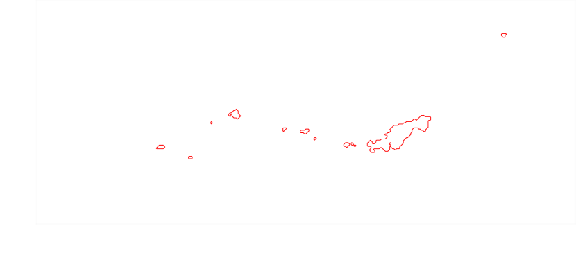
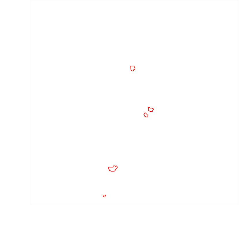
Since we have at our disposal the covariance map of these measurements, we have assessed the reliability of each density peak in these figures. The red contours in the figures show the areas (larger than 2 pixels) where the local YSO density exceeds $1.5\text{\,}\mathrm{s}\mathrm{t}\mathrm{a}\mathrm{r}\mathrm{s}\mathrm{/}\mathrm{p}\mathrm{i}\mathrm{x}\mathrm{e}\mathrm{l}$, corresponding approximately to a signal-to-noise ratio larger than 3.5: note how some regions in black in Fig. 10 do not reach the threshold because of the large error associated with them (mostly due to the high extinction values there).

Table 3 shows the YSO clusters identified in the Orion A and B areas using our simple prescription, together with the most relevant parameters. In some cases we clearly see that angularly close clusters appear as a single contour in our maps: the simple procedure used here to define clusters, the relatively coarse resolution used, and the cluster morphology itself prevent us from deblending some close objects. An extreme case of this situation might be the ISF (the Integral Shaped Filament) cluster, where the limitations due to angular resolution would make it difficult to resolve and separate smaller clusters if they exist in such a very populous region. We note that the ISF cluster encompasses M42, the Trapezium and ONC clusters as well as an extended population of YSOs along the ISF.

The radius $R$ reported in the table corresponds to the radius of a circle that would occupy the same area as the identified cluster, i.e. to the connected region of the sky where the inferred density of YSOs exceeds the background by $3\sigma$. At the estimated distance of Orion, $413\text{\,}\mathrm{p}\mathrm{c}$ (Reid et al., 2009), $1^{\prime}$ corresponds to $0.12\text{\,}\mathrm{p}\mathrm{c}$: therefore, the clusters identified have radii spanning from $\sim$2.4\text{\,}\mathrm{p}\mathrm{c}$$ to $\sim$0.15\text{\,}\mathrm{p}\mathrm{c}$$.

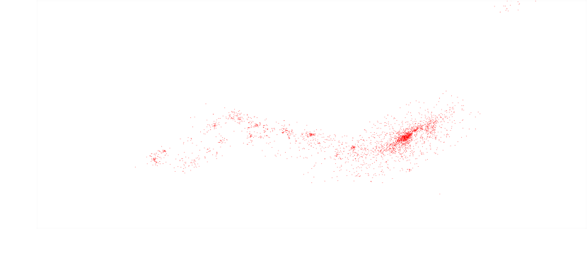
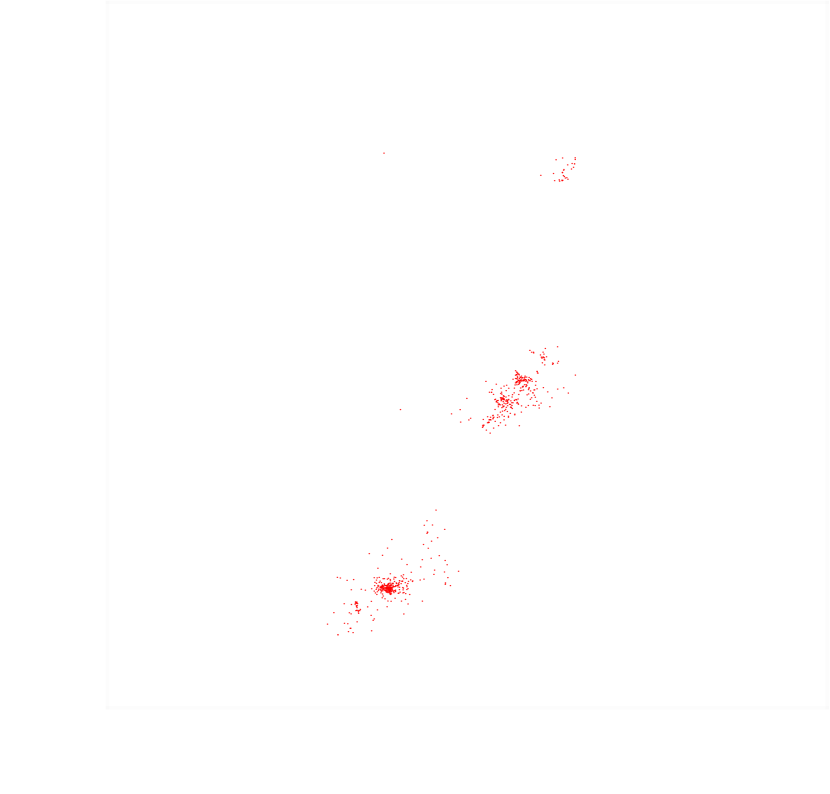
The well known clusters in these clouds are correctly identified by our procedure. It is interesting to compare Table 3 with clusters identified independently using much more secure data. Among the ones at our disposal, the recent catalog of embedded YSOs obtained by Megeath et al. (2016) using the Spitzer Space Telescope and the Chandra observatory is probably the most secure and complete: we will therefore focus on this catalog. Since our definition of a cluster is based on an somewhat arbitrary parameters (signal-to-noise threshold, minimum number of pixels, no correction for the stars missed at the boundaries), and since different, more-or-less, arbitrary parameters are also used by Megeath et al. (2016), we find it more appropriate and fair to make a comparison after we first homogenize the data. Specifically, we take Megeath et al. (2016) YSO list and we make out of it a density map using a Gaussian kernel of the same size of the one used for our map. Figures 12 and 13 show the results obtained for Orion A and B, which clearly compares very well with our own maps, derived purely from the 2MASS point source catalog. The most relevant structures are present in both maps and have very similar shapes; the only differences are the noise present in our maps (however at a relatively low level), and the limited coverange of the Spitzer derived density maps.

The qualitative similarity of these maps can be quantified if compare clusters identified in both maps using the same criteria. Table 4 shows a list of clusters identified in the smoothed Megeath et al. (2016) maps using a fix density threshold (set to $1.5\text{\,}\mathrm{s}\mathrm{t}\mathrm{a}\mathrm{r}\mathrm{s}\mathrm{/}\mathrm{p}\mathrm{i}\mathrm{x}\mathrm{e}\mathrm{l}$). In this table we compare the number of Spitzer YSOs with the number of YSOs predicted from the integral of the $\sigma_{\mathrm{YSOs}}$ over the area of each cluster as defined from Megeath et al. density map, together with the computed $1$-$\sigma$ error. It is clear that in almost all cases we find an excellent agreement, although in many cases our estimates are slightly larger than the ones by Megeath et al. We can speculate that this is due to the presence of class III YSO, which likely would be missed by Spitzer. Indeed, a comparison of the two panels of Fig. 12 shows that the bottom panel, corresponding to our density map, has spatially more extended clusters than the top panel, corresponding to Megeath et al. density map.

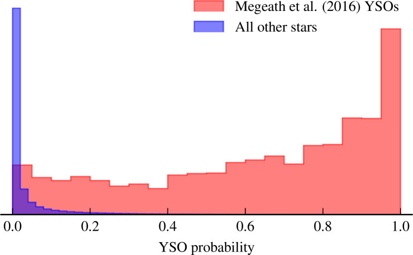
As discussed earlier on, our algorithm is a statistical one and works best when it is applied to a sizeable number of stars. However, we can also push it and associate to each single star a probability of being a YSO: to this purpose, for the $n$-th star we can compute

$$P_{i}=\frac{\sigma_{i}(\@vec{x}_{n})p_{i}(m_{n}-A_{n})}{\sum_{j=1}^{L}\sigma_{j}(\@vec{x}_{n})p_{j}(m_{n}-A_{n})}\;.$$ (35)

Note how this quantity resembles the term within the outer sum of Eq. (30). Figure 14 shows the distribution of $P_{\mathrm{YSO}}$ (that is, the distribution in the probabilities assigned to each object to be a YSO) for the Megeath et al. (2016) YSO candidates and for all the other objects. It is clear how all the other objects have $P_{\mathrm{YSO}}$ that is concentrated around zero, while the YSO candidates have a much broader distribution that extends to unity. For these latter objects the distribution, in addition to a substal peak at $P_{\mathrm{YSO}}=1$, shows a long tail up to small values of $P_{\mathrm{YSO}}$: this is not unexpected, since our identification is only statistical (and therefore we cannot identify unambigously YSOs). Note also how the relatively low values of $P_{\mathrm{YSO}}$ for some genuine YSOs in our algorithm are compensated by the small tail in the distribution of field stars (this works because there are many more field stars than YSOs, a fact that is accounted for in the algorithm).

5.1 Sensitivity to the distributed population

Recently, Kubiak et al., 2016, have identified a rich and well-defined stellar population of about 2 000 objects, mostly M stars without extinction or infrared-excesses, as the low-mass counterpart to the Orion OB Ib subgroup (the Orion belt population). This low-mass population is not obviously clustered but instead appears to be distributed across $\sim 10$ square degrees and the authors speculate that it could represent the evolved counterpart of a Orion nebula-like cluster. While more data is needed to test this scenario, it is clear that much can be learned about the origin of stellar OB associations and the dispersal of clusters into the Galactic field if one is able to trace in a robust manner the distribution of the slightly older and more expanded populations surrounding star-forming molecular clouds.

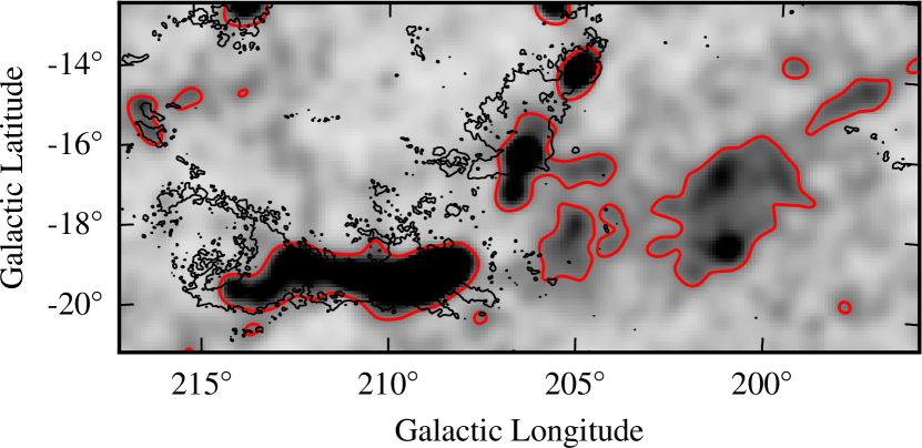
We now investigate the extent to which the technique proposed here is suitable for detection of looser, more expanded distributions of young stars, in particular the low-mass counterpart to the Orion OB association presented in Kubiak et al., 2016. For this purpose, we have built a lower resolution map of the region, employing a FWHM of $30\text{\,}\mathrm{a}\mathrm{r}\mathrm{c}\mathrm{m}\mathrm{i}\mathrm{n}$.

Figure 15 shows that, surprisingly, we are well able to recover the stellar over-density of the Ori Ib population, and for the first time, the stellar over-density of the Ori Ia population. These over-densities are likely to be created by low-mass stars as 2MASS is still sensitive to the peak of the IMF for the putative distance and age of these subgroups. An analysis of the substructure seen in the distributed population visible in Figure 15 above the noise pattern is beyond the scope of this paper, but will best addressed once Gaia parallaxes are generally available. Of relevance for this paper is that the ability of the method to trace the dispersed population from existing all sky data opens a new window on the unsolved problem of the origins of OB association and cluster dispersal in to the field.

6 Conclusions

The following items summarize the main results presented in this paper:

• We have developed a new method to discover and characterize deeply embedded star clusters.

• The method is able to statistically classify objects as field stars or YSOs and corrects for the effects of differential extinction.

• We have provided expressions for the covariance of the inferred densities and we have validated both the method and the analytic expression for the covariance with a set of simple but realistic simulations.

• We have applied the new method to 2MASS point sources observed in the Orion A and B and we have shown that we can identify and characterize well protostellar clusters in these regions, as well as detect much looser associations such as the OB 1a and 1b subgroups.

Finally, we note that the method proposed here can be easily extended to multi-band observations by using suitable probability distributions $p_{i}(\@vec{m})$ for various populations as a function of the magnitude vector $\@vec{m}$. Its implementation would be essentially identical, with minor modifications to take into account the different effects of extinction on different bands. The natural use of such an extension would be in the context of techniques such as the one proposed by Juvela & Montillaud (2016) which are able to recover the extinction from a complex analysis of multi-band data.

Appendix A Implementation

In this section we consider a few details and analytical expressions useful to evaluate some of the expressions needed to implement the method proposed here.

A.1 Algorithm

The algorithm proposed in this paper is essentially an iterative application of Eq. (30) to the set of densities $\{\sigma_{i}(\@vec{x})\}$. A few notes, however, are necessary to better implement the algorithm:

• The method assumes that the extinction values in the $H$ band are available for each star used. In our implementation these values are obtained through the use of the Nicer algorithm. Other techniques can be used, as long as the extinction is refereed to the single star and is not an average extinction at the location of the star. In our implementation, this requirement limits the method to stars for which, in addition to the $H$-band measurements, have at least another band photometry.

• Since the various densities are spatially variable, one needs to repeat the iteration of Eq. (30) to each point in the map.

• Equation (30) itself needs to be iterated a few times (typically around ten, in some cases a little more) before reaching a good convergence. This generally suggests the use of simple analytical models for the various functions involved in this equation (the probability distributions $p_{i}(m)$ and the completeness function $c(m)$, discussed below).

A.2 H-band probability distributions and completeness function

Figure 16: An histogram of $H$ band magnitudes of stars in a control field region, together with its best fit (an exponential with a complementary error function truncation, see the text).

In this paper we have considered two useful models for the $H$-band luminosity function: the exponential distribution and the normal (Gaussian) one.

We parametrize the exponential distribution as

$$p(m)=k\beta\mathrm{e}^{\beta m}\propto 10^{\alpha m}\;,$$ (36)

where $k$ is a normalization constant that will be found lather on and $\beta=\alpha\ln 10$.

The normal distribution is parametrized as

$$p(m)=\frac{k}{\sqrt{2\pi s^{2}}}\mathrm{e}^{-(m-m_{0})^{2}/2s^{2}}\;,$$ (37)

where again $k$ is a normalization constant to be investigated later.

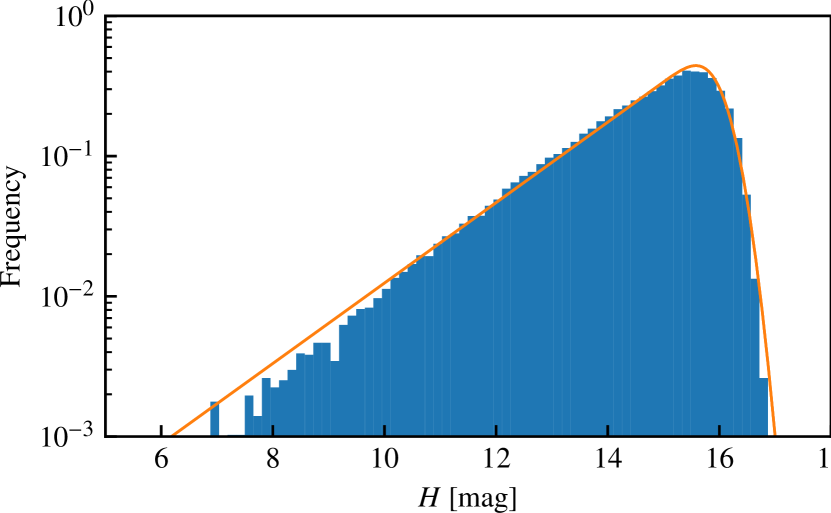
Finally, we model the completeness function $c(m)$ in terms of the complementary error function $\operatorname{erfc}$. This can justified from an empirical point of view since the error function has a shape that resemble the completeness function. It is also reasonable from a statistical point of view if the photometric errors are Gaussian: in this case, one can suppose that the probability that an object be detected is an integral over a relevant part of the Gaussian. Specifically, we assume for $c(m)$ the following functional form:

$$c(m)=\frac{1}{2}\operatorname{erfc}\left(\frac{m-m_{\mathrm{c}}}{\sqrt{2\sigma^{2}_{\mathrm{c}}}}\right)\;,$$ (38)

where $m_{\mathrm{c}}$ is the 50% completeness limit and $\sigma_{\mathrm{c}}$ sets the width of the completeness function. Figure 16 shows that our simple model for the control field HLF, the product of $p(m)c(m)$ with $p(m)$ following an exponential distribution and $c(m)$ described in terms of an erfc, reproduces well the data.

A.3 Statistical errors and completeness function

As noted above, statistical errors can be included in our algorithm by convolving the probability distributions $p_{i}$ with appropriate kernels. We expect to have two main sources for statistical errors: photometric errors in the $H$-band magnitude measurements and errors in the extinction measurements. While the formers are relatively simple to characterize (typically, they will be provided in the star catalogue), the latter are a combination of different sources of errors: the scatter in the intrinsic color of sources and the photometric errors in each band used. If extinctions are derived using the Nicer algorithm, as assumed here, then the variance associated to each extinction measurement can be computed from the expression

$$\operatorname{Var}(A)\equiv\sigma^{2}_{A}=\frac{1}{\@vec{k}^{T}C^{-1}\@vec{k}}\;,$$ (39)

where, following the notation of Lombardi & Alves (2001), we have called $\@vec{k}$ is the reddening vector and $C$ the combined covariance matrix of the observed colors (including both the intrinsic scatter in the color of unextinguished stars and the individual photometric errors).

Looking again at Eq. (30), i.e. the main equation representing our method, we see that in reality the $H$-band magnitudes and the associated extinction measurements typically enter the problem through the combination $m-A$; moreover, while in the numerator the combination is $m_{n}-A_{n}$ and involves therefore measurements of both $m$ and $A$ for individual stars, in the denominator the combination is $m-A_{n}$, with $m$ integration variable. Therefore, in presence of errors these two parts of the expression must be computed separately.

Let us consider first the denominator. Since there the only argument of $p_{i}$ with associated errors is $A_{n}$, the measured extinction for the $n$-th star, we just need to convolve the magnitude distribution with a Gaussian kernel with variance provided by Eq. (39).

In the case of the numerator the situation is slightly more complicated, because there we find the combination $m_{n}-A_{n}$. Since $A_{n}$ is computed from the observed magnitude of each star (including of course the $H$-band magnitude), $m_{n}$ and $A_{n}$ are correlated. A simple calculation shows that the variance associated to the combination $m_{n}-A_{n}$ is

$$\operatorname{Var}(m_{n}-A_{n})=k_{H}^{2}\sigma^{2}_{A}+\sigma^{2}_{H}\bigl{[}1-2\,(b_{J-H}-b_{H-K})\,k_{H}\bigr{]}\;.$$ (40)

In this expression the last term is related to the correlation between $A$ and $m$ and is equal to $\sigma^{2}_{H}$, the square of the photometric error on the $H$-band magnitude. The factors $b_{J-H}$ and $b_{H-K}$ are quantities that can be computed from Eq. (12) of Lombardi & Alves (2001), while $k_{H}$ is the reddening vector for the $H$ band, i.e. the ratio $A_{H}/A$.

A.4 Convolution integrals

The convolution of the luminosity functions (36) and (37) with Gaussian kernels representing the statistical errors take simple forms. Calling $\sigma^{2}_{p}$ the variance of the convolution kernel, given depending on the term by Eq. (39) or by Eq. (40), and using the tilde to represent the convolved $H$-band luminosity functions, we find for the exponential distribution

$$\tilde{p}(m)=k\beta\mathrm{e}^{\beta m+\sigma^{2}_{p}\beta^{2}/2}\;.$$ (41)

Similarly, for the Gaussian model we find

$$\tilde{p}(m)=\frac{k}{\sqrt{2\pi(s^{2}+\sigma^{2}_{p})}}\mathrm{e}^{-(m-m_{0})^{2}/2(s^{2}+\sigma^{2}_{p})}\;,$$ (42)

A.5 Completeness integrals

Finally, we need to compute the integral in the denominator of Eq. (30), involving the $H$-band luminosity function $p(m)$ and the completeness function $c(m)$. A simple change of variable casts this integral (similar to a convolution) into a more convenient form:

$$\int c(m)p(m-A)\,\mathrm{d}m=\int c(m+A)p(m)\,\mathrm{d}m\equiv K(A)\;.$$ (43)

In this equation we have called $K(A)$ the result of the integral, retaining its explicit dependence on $A$. We now consider the derivative $K^{\prime}$ of $K$:

$$K^{\prime}(A)=\int c^{\prime}(m+A)p(m)\,\mathrm{d}m\;,$$ (44)

and note that, since $c$ is the error function, $c^{\prime}$ is a Gaussian function. Since Eq. (44) is also (essentially) a convolution, this allows us to compute $K^{\prime}(A)$ using formulae similar to the ones of the previous section: as a result, we see that $K^{\prime}(A)$ remains either an exponential or a Gaussian, depending on the function form of $p(m)$.

Finally, we need to integrate back $K^{\prime}(A)$ to obtain $K$. The result we obtain from this procedure is, in case of an exponential distribution,

$$K(A)=k\mathrm{e}^{\beta(m_{\mathrm{c}}-A)+\sigma^{2}_{\mathrm{c}}\beta^{2}/2}\;.$$ (45)

For the Gaussian distribution the result contains again the error function:

$$K(A)=\frac{k}{2}\operatorname{erfc}\left(\frac{m_{0}-m_{\mathrm{c}}+A}{\sqrt{2(\sigma_{\mathrm{c}}^{2}+s^{2})}}\right)\;.$$ (46)

If statistical errors have to be taken into account, these expressions simply change into

$$K(A)=k\mathrm{e}^{\beta(m_{\mathrm{c}}-A)+(\sigma^{2}_{\mathrm{c}}+\sigma^{2}_{p})\beta^{2}/2}\;,$$ (47)

and

$$K(A)=\frac{k}{2}\operatorname{erfc}\left(\frac{m_{0}-m_{\mathrm{c}}+A}{\sqrt{2(\sigma_{\mathrm{c}}^{2}+s^{2}+\smash[b]{\sigma^{2}_{p}})}}\right)\;.$$ (48)

References

- Bressert et al. (2010) Bressert, E., Bastian, N., Gutermuth, R., et al. 2010, MNRAS, 409, L54
- Cambrésy et al. (2002) Cambrésy, L., Beichman, C. A., Jarrett, T. H., & Cutri, R. M. 2002, AJ, 123, 2559
- Cambrésy et al. (2013) Cambrésy, L., Marton, G., Feher, O., Tóth, L. V., & Schneider, N. 2013, A&A, 557, A29
- Cambrésy et al. (2006) Cambrésy, L., Petropoulou, V., Kontizas, M., & Kontizas, E. 2006, A&A, 445, 999
- Carpenter (2000) Carpenter, J. M. 2000, AJ, 120, 3139
- Casertano & Hut (1985) Casertano, S. & Hut, P. 1985, ApJ, 298, 80
- Feigelson & Babu (2012) Feigelson, E. D. & Babu, G. J. 2012, Modern Statistical Methods for Astronomy (Cambridge University Press)
- Geyer & Burkert (2001) Geyer, M. P. & Burkert, A. 2001, MNRAS, 323, 988
- Gutermuth et al. (2009) Gutermuth, R. A., Megeath, S. T., Myers, P. C., et al. 2009, ApJS, 184, 18
- Gutermuth et al. (2005) Gutermuth, R. A., Megeath, S. T., Pipher, J. L., et al. 2005, ApJ, 632, 397
- Hubble (1926) Hubble, E. P. 1926, ApJ, 64
- Juvela & Montillaud (2016) Juvela, M. & Montillaud, J. 2016, A&A, 585, A78
- Kubiak et al. (2016) Kubiak, K., Alves, J., Bouy, H., et al. 2016, ArXiv e-prints
- Lada & Lada (2003) Lada, C. J. & Lada, E. A. 2003, ARA&A, 41, 57
- Lada et al. (1984) Lada, C. J., Margulis, M., & Dearborn, D. 1984, ApJ, 285, 141
- Lada et al. (1991) Lada, E. A., Depoy, D. L., Evans, II, N. J., & Gatley, I. 1991, ApJ, 371, 171
- Lane et al. (2016) Lane, J., Kirk, H., Johnstone, D., et al. 2016, ArXiv e-prints
- Lombardi (2009) Lombardi, M. 2009, A&A, 493, 735
- Lombardi & Alves (2001) Lombardi, M. & Alves, J. 2001, A&A, 377, 1023
- Lombardi et al. (2011) Lombardi, M., Alves, J., & Lada, C. J. 2011, A&A, 535, A16
- Lombardi et al. (2013) Lombardi, M., Lada, C. J., & Alves, J. 2013, A&A, 559, A90
- MacKay (2003) MacKay, D. 2003, Information Theory, Inference, and Learning Algorithms (Cambridge University Press)
- Megeath et al. (2012) Megeath, S. T., Gutermuth, R., Muzerolle, J., et al. 2012, AJ, 144, 192
- Megeath et al. (2016) Megeath, S. T., Gutermuth, R., Muzerolle, J., et al. 2016, AJ, 151, 5
- Meingast et al. (2016) Meingast, S., Alves, J., Mardones, D., et al. 2016, A&A, 587, A153
- Muench et al. (2002) Muench, A. A., Lada, E. A., Lada, C. J., & Alves, J. 2002, ApJ, 573, 366
- Prisinzano et al. (2008) Prisinzano, L., Micela, G., Flaccomio, E., et al. 2008, ApJ, 677, 401
- Reid et al. (2009) Reid, M. J., Menten, K. M., Zheng, X. W., et al. 2009, ApJ, 700, 137
- Román-Zúñiga et al. (2008) Román-Zúñiga, C. G., Elston, R., Ferreira, B., & Lada, E. A. 2008, ApJ, 672, 861
- von Hoerner (1963) von Hoerner, S. 1963, ZAp, 57, 47
- Wilking & Lada (1985) Wilking, B. A. & Lada, C. J. 1985, in Protostars and Planets II, ed. D. C. Black & M. S. Matthews, 297–319