institutetext: a𝑎\,{}^{a}Niels Bohr International Academy and Discovery Center, University of Copenhagen
Blegdamsvej 17, DK-2100 Copenhagen , Denmark,
bUniversidad Santiago de Cali, Facultad de Ciencias Basicas,
Campus Pampalinda, Calle 5 No. 62-00, Código postal 76001, Santiago de Cali, Colombia
institutetext: cInstitut de Ciencies del Cosmos, Universitat de Barcelona (IEEC-UB),
Marti i Franques 1, Barcelona 08028, Spain

One-loop Parke-Taylor factors for quadratic propagators from massless scattering equations

Humberto Gomez,a,b Cristhiam Lopez-Arcosb and Pedro Talaverac humgomzu@gmail.com, crismalo@gmail.com, peterbretons@gmail.com
Abstract

In this paper we reconsider the Cachazo-He-Yuan construction (CHY) of the so called scattering amplitudes at one-loop, in order to obtain quadratic propagators. In theories with colour ordering the key ingredient is the redefinition of the Parke-Taylor factors. After classifying all the possible one-loop CHY-integrands we conjecture a new one-loop amplitude for the massless Bi-adjoint Φ3superscriptΦ3\Phi^{3} theory. The prescription directly reproduces the quadratic propagators of the traditional Feynman approach.

1 Introduction

Our most accurate knowledge on quantum field theory in Minkowski (3+1)31(3+1)-d is almost entirely based on perturbation methods. At leading order, quantities such as scattering amplitudes are computed by adding tree-like diagrams. Even this elementary manipulation becomes a formidable task at rather low multiplicity kinematics and become only technically feasible by using the Weyl-van der Waerden spinor calculus.

The use of on-shell methods for the calculation of scattering amplitudes has come into attention since the last decade, following Witten’s seminal work Witten:2003nn . A remarkable development following these ideas is the approach by Cachazo-He-Yuan (CHY) Cachazo:2013gna ; Cachazo:2013hca , it has the great advantages of being applicable to several dimensions and also to a large array of theories Cachazo:2013iea ; Cachazo:2014xea ; Cachazo:2014nsa ; Cachazo:2016njl , even beyond field theory Mizera:2017sen ; Mizera:2017cqs . The main ingredient for this approach are the tree-level scattering equations Cachazo:2013gna

Ea:=bakakbσab=0,σab:=σaσb,a=1,2,,n,formulae-sequenceassignsubscript𝐸𝑎subscript𝑏𝑎subscript𝑘𝑎subscript𝑘𝑏subscript𝜎𝑎𝑏0formulae-sequenceassignsubscript𝜎𝑎𝑏subscript𝜎𝑎subscript𝜎𝑏𝑎12𝑛\displaystyle E_{a}:=\sum_{b\neq a}\frac{k_{a}\cdot k_{b}}{\sigma_{ab}}=0,\quad\sigma_{ab}:=\sigma_{a}-\sigma_{b},\quad a=1,2,\ldots,n, (1)

where the σasubscript𝜎𝑎\sigma_{a}’s denote punctures on the sphere. The tree-level S-matrix can be written in terms of contour integrals localized over solutions of these equations on the moduli space of n-punctured Riemann spheres

𝒜n=Γ𝑑μntreetreeCHY(σ),subscript𝒜𝑛subscriptΓdifferential-dsuperscriptsubscript𝜇𝑛treesuperscriptsubscripttreeCHY𝜎\displaystyle{\cal A}_{n}=\int_{\Gamma}\,d\mu_{n}^{\rm tree}\,\,\cal{I}_{\rm tree}^{\rm CHY}(\sigma), (2)

where the integration measure, dμntree𝑑superscriptsubscript𝜇𝑛treed\mu_{n}^{\rm tree}, is given by

dμntree=a=1ndσaVol(PSL(2,))×(σijσjkσki)bi,j,knEb𝑑superscriptsubscript𝜇𝑛treesuperscriptsubscriptproduct𝑎1𝑛𝑑subscript𝜎𝑎VolPSL2subscript𝜎𝑖𝑗subscript𝜎𝑗𝑘subscript𝜎𝑘𝑖superscriptsubscriptproduct𝑏𝑖𝑗𝑘𝑛subscript𝐸𝑏d\mu_{n}^{\rm tree}=\frac{\prod_{a=1}^{n}d\sigma_{a}}{{\rm Vol}\,({\rm PSL}(2,\mathbb{C}))}\times\frac{(\sigma_{ij}\sigma_{jk}\sigma_{ki})}{\prod_{b\neq i,j,k}^{n}E_{b}} (3)

and the contour ΓΓ\Gamma is defined by the n3𝑛3n-3 independent scattering equations

Eb=0,bi,j,k.formulae-sequencesubscript𝐸𝑏0𝑏𝑖𝑗𝑘E_{b}=0,\quad b\neq i,j,k\,. (4)

The integrand, treeCHYsuperscriptsubscripttreeCHY\cal{I}_{\rm tree}^{\rm CHY}, depends on the described theory. There are other approaches that use the same moduli space Witten:2003nn ; Roiban:2004yf ; Cachazo:2012da ; Cachazo:2012kg , but restricted to four dimensions.

There have been developed several methods to evaluate the integrals, from different perspectives. Some approaches study the solutions to the scattering equations for particular kinematics and/or dimensions Cachazo:2013iaa ; Cachazo:2013iea ; Kalousios:2013eca ; Lam:2014tga ; Cachazo:2016sdc ; He:2016vfi ; Cachazo:2015nwa ; Cachazo:2016ror , others work with a polynomial form Kalousios:2015fya ; Dolan:2014ega ; Dolan:2015iln ; Huang:2015yka ; Cardona:2015ouc ; Cardona:2015eba ; Sogaard:2015dba ; Bosma:2016ttj ; Zlotnikov:2016wtk ; Mafra:2016ltu , or formulating sets of integration rules Baadsgaard:2015ifa ; Baadsgaard:2015voa ; Huang:2016zzb ; Cardona:2016gon ; Zhou:2017mfj . A different approach was proposed in Gomez:2016bmv , taking the double covered version of the sphere, the so called ΛΛ\Lambda-algorithm, which we will employ in this work.

A generalization for loop level of the CHY formalism has been made. The ambitwistor and pure spinor ambitwistor worldsheet Mason:2013sva ; Berkovits:2013xba provided a prescription for a generalization to higher genus Riemann surfaces Geyer:2015bja ; Geyer:2015jch ; Adamo:2015hoa . A different approach was also developed in Cachazo:2015aol ; He:2015yua ; Baadsgaard:2015hia , where the forward limit with two more massive particles, playing the role of the loop momenta, were introduced. The scattering equations for massive particles were already studied in Dolan:2013isa ; Naculich:2014naa . Another alternative approach using an elliptic curve was developed in Cardona:2016wcr ; Cardona:2016bpi .

The previous prescriptions give a new representation of the Feynman integrals with propagators linear in loop momenta. In order to find the equivalence with the usual Feynman propagators, (+K)2superscript𝐾2(\ell+K)^{-2}, two additional steps must be taken: the first one is the use of partial fractions, and the second one is the shifting of loop momenta Geyer:2015jch ; Casali:2014hfa .

Recently, one of the authors Gomez:2017lhy proposed a different approach to obtain the quadratic Feynman propagators directly from the CHY-integrands for the scalar Φ3superscriptΦ3\Phi^{3} theory111There are some overlapping ideas with the recent paper published by Farrow and Lipstein Farrow:2017eol .. The motivation came by analysing a Riemann surface of genus two after an unitary cut, which look exactly like a tree level diagram before the forward limit, but instead of the two massive particles associated to the loop momenta there are four massless particles. This new approach allows to work again with the scattering equations for massless particles, but at the expenses of increasing the number to n+4𝑛4n+4. In addition there is also the need to introduce a new measure of integrations that guarantees the cut and then take the forward limit.

In the present work, we follow the line of thought of Gomez:2017lhy and propose a reformulation for the one-loop Parke-Taylor factors. Splitting the massive loop momenta (+,)superscriptsuperscript(\ell^{+},\ell^{-}) into the four massless ones ((a1,b1),(b2,a2))subscript𝑎1subscript𝑏1subscript𝑏2subscript𝑎2((a_{1},b_{1}),(b_{2},a_{2})), we will have one-loop Parke-Taylor factors that will enter into CHY-integrands to lead directly to the usual Feynman propagators. The CHY-integrands in question are the ones for the Bi-adjoint Φ3superscriptΦ3\Phi^{3} scalar theory.

Outline

This paper is organized as follows. In section 2 we present our reformulation of the one-loop Parke-Taylor factors (PT). The expression is written in terms of the generalized holomorphic one-form on the Torus, ωi:ja:bsubscriptsuperscript𝜔:𝑎𝑏:𝑖𝑗\omega^{a:b}_{i:j}. By exploiting algebraic identities we formulate the Theorem 1: each term in the PT factors can be decomposed into terms containing at least two ωi:ja:bsubscriptsuperscript𝜔:𝑎𝑏:𝑖𝑗\omega^{a:b}_{i:j} factors, i.e. the PT factors are rearranged in an expansion manifestly tadpole-free222As it will be explained, the number of ωi:ja:bsubscriptsuperscript𝜔:𝑎𝑏:𝑖𝑗\omega^{a:b}_{i:j} is related with the polygon of the loop, for example, two ωi:ja:bsubscriptsuperscript𝜔:𝑎𝑏:𝑖𝑗\omega^{a:b}_{i:j} in the left integrand can only generate a bubble or a triangle. .

In section 3 we write, classify and match with their Feynman integrands counterparts, some general type of CHY-integrands that can appear at one-loop level. Since we are working with n+4𝑛4n+4 massless particles, the contour integrals can be calculated using any of the existing methods of integration. As we have mentioned already we employ the so-called ΛΛ\Lambda-algorithm, with the choice of a new gauge fixing, to solve them. This allows to analytically evaluate arbitrary CHY-integrals using simple graphical rules. The classification is made tracing the structures defined in section 2. As will become clear each element inside the partial amplitude have an unambigous correspondence with the elements of the CHY-graphs, starting with the n-gon, then following with the ones with tree level structures attached to their corners.

Section 4 shows our proposal for the partial amplitude of the Bi-adjoint Φ3superscriptΦ3\Phi^{3} theory at one-loop with quadratic propagators: first we give a simple review at tree level and one-loop with linear propagators, then we propose our formula using our definition for the PT factors.

In order to support our proposition in section 5 we perform explicitly the calculation for the partial amplitudes of the three and four-point functions. We make an extensive use of the results of previous sections. In particular we emphasize the direct interpretation of the CHY-integrals in terms of Feynman diagrams. This mapping is codified in the following equality at the integrand level

12N+1𝑑Ω×sa1b1×𝑑μN+4tree1superscript2𝑁1differential-dΩsubscript𝑠subscript𝑎1subscript𝑏1differential-dsubscriptsuperscript𝜇tree𝑁4\frac{1}{2^{N+1}}\int d\Omega\times s_{a_{1}b_{1}}\times\int d\mu^{\rm tree}_{N+4} [Uncaptioned image] = [Uncaptioned image]

that constitutes one of the most important results of this work and it will be explained in detail during the course of this paper.

In section 6 we comment on the issue of the external-leg bubble contributions. Diagrams involved are singular and need to be regularized. Next section, 7, is for illustrative purposes and is devoted to the iϵ𝑖italic-ϵi\epsilon prescription and how to directly obtain it by dimension reduction. Finally, in section 8 we conclude by summarizing our findings.

For not disrupting the line of the paper more technical discussions have been gathered in some appendices: In Appendix A we explicitly show the sufficient form of the measure (20) to tackle the one-loop CHY-integral prescription. In particular how the momenta combination it contains arrises. Proof of Theorem 1 is casted in Appendix B where it is discussed at length. Appendix C collects the relation between some techniques developed across the paper and the linear propagator prescription. We conclude by probing an statement of Cardona:2016bpi .

Before beginning section 2, we define the notation that is going to be used in the paper.

Notation

For convenience, in this paper we use the following notation

σij:=σiσj,ωi:ja:b:=σabσiaσjb.formulae-sequenceassignsubscript𝜎𝑖𝑗subscript𝜎𝑖subscript𝜎𝑗assignsuperscriptsubscript𝜔:𝑖𝑗:𝑎𝑏subscript𝜎𝑎𝑏subscript𝜎𝑖𝑎subscript𝜎𝑗𝑏\displaystyle\sigma_{ij}:=\sigma_{i}-\sigma_{j},\qquad\qquad\omega_{i:j}^{a:b}:=\frac{\sigma_{ab}}{\sigma_{ia}\,\,\sigma_{jb}}. (5)

Note that ωi:ja:bsuperscriptsubscript𝜔:𝑖𝑗:𝑎𝑏\omega_{i:j}^{a:b} are the generalization of the (1,0)limit-from10(1,0)-forms used in Gomez:2016cqb to write the CHY-integrands at two-loop. In addition, we define the σabsubscript𝜎𝑎𝑏\sigma_{ab}’s and ωi:ja:bsuperscriptsubscript𝜔:𝑖𝑗:𝑎𝑏\omega_{i:j}^{a:b}’s chains as

(i1,i2,,ip):=σi1i2σip1ipσipi1,assignsubscript𝑖1subscript𝑖2subscript𝑖𝑝subscript𝜎subscript𝑖1subscript𝑖2subscript𝜎subscript𝑖𝑝1subscript𝑖𝑝subscript𝜎subscript𝑖𝑝subscript𝑖1\displaystyle(i_{1},i_{2},\ldots,i_{p}):=\sigma_{i_{1}i_{2}}\cdots\sigma_{i_{p-1}i_{p}}\sigma_{i_{p}i_{1}}, (6)
(i1,i2,,ip)ωa:b:=ωi1:i2a:bωip1:ipa:bωip:i1a:bassignsubscriptsuperscriptsubscript𝑖1subscript𝑖2subscript𝑖𝑝:𝑎𝑏𝜔subscriptsuperscript𝜔:𝑎𝑏:subscript𝑖1subscript𝑖2subscriptsuperscript𝜔:𝑎𝑏:subscript𝑖𝑝1subscript𝑖𝑝superscriptsubscript𝜔:subscript𝑖𝑝subscript𝑖1:𝑎𝑏\displaystyle(i_{1},i_{2},\ldots,i_{p})^{a:b}_{\omega}:=\omega^{a:b}_{i_{1}:i_{2}}\cdots\omega^{a:b}_{i_{p-1}:i_{p}}\omega_{i_{p}:i_{1}}^{a:b}
=ωi1:i1a:bωip1:ip1a:bωip:ipa:b,absentsubscriptsuperscript𝜔:𝑎𝑏:subscript𝑖1subscript𝑖1subscriptsuperscript𝜔:𝑎𝑏:subscript𝑖𝑝1subscript𝑖𝑝1superscriptsubscript𝜔:subscript𝑖𝑝subscript𝑖𝑝:𝑎𝑏\displaystyle\qquad\qquad\qquad\quad=\omega^{a:b}_{i_{1}:i_{1}}\cdots\omega^{a:b}_{i_{p-1}:i_{p-1}}\omega_{i_{p}:i_{p}}^{a:b},
(i1σ,i2σ,,imω,im+1σ,,inω,ipσ)a:b:=σi1i2σi2i3ωimim+1a:bσim+1im+2ωinin+1a:bσip1ipσipi1.assignsuperscriptsuperscriptsubscript𝑖1𝜎subscriptsuperscript𝑖𝜎2superscriptsubscript𝑖𝑚𝜔superscriptsubscript𝑖𝑚1𝜎superscriptsubscript𝑖𝑛𝜔superscriptsubscript𝑖𝑝𝜎:𝑎𝑏subscript𝜎subscript𝑖1subscript𝑖2subscript𝜎subscript𝑖2subscript𝑖3subscriptsuperscript𝜔:𝑎𝑏subscript𝑖𝑚subscript𝑖𝑚1subscript𝜎subscript𝑖𝑚1subscript𝑖𝑚2subscriptsuperscript𝜔:𝑎𝑏subscript𝑖𝑛subscript𝑖𝑛1subscript𝜎subscript𝑖𝑝1subscript𝑖𝑝subscript𝜎subscript𝑖𝑝subscript𝑖1\displaystyle(i_{1}^{\sigma},i^{\sigma}_{2},\ldots,i_{m}^{\omega},i_{m+1}^{\sigma},\ldots,i_{n}^{\omega},\ldots i_{p}^{\sigma})^{a:b}:=\sigma_{i_{1}i_{2}}\sigma_{i_{2}i_{3}}\cdots\omega^{a:b}_{i_{m}i_{m+1}}\sigma_{i_{m+1}i_{m+2}}\cdots\omega^{a:b}_{i_{n}i_{n+1}}\cdots\sigma_{i_{p-1}i_{p}}\sigma_{i_{p}i_{1}}.

In order to have a graphical description for the CHY-integrands on a Riemann sphere (CHY-graphs), it is useful to represent each σasubscript𝜎𝑎\sigma_{a} puncture as a vertex, the factor 1σab1subscript𝜎𝑎𝑏{1\over\sigma_{ab}} as a line and the factor σabsubscript𝜎𝑎𝑏\sigma_{ab} as a dashed line that we call the anti-line. Additionally, since we often use the Λlimit-fromΛ\Lambda-algorithm333It is useful to recall that the Λlimit-fromΛ\Lambda-algorithm fixes four punctures, three of them by the PSL(2,)PSL2{\rm PSL}(2,\mathbb{C}) symmetry and the last one by the scale invariance. Gomez:2016bmv we introduce the color code given in Fig. 1 and 2 for a mnemonic understanding.

Refer to caption
Figure 1: Vertex Color code in CHY-graphs for the Λlimit-fromΛ\Lambda-algorithm.
Refer to caption
Figure 2: Edges Color code in CHY-graphs for the Λlimit-fromΛ\Lambda-algorithm.

Finally, we introduce the momenta notation

k{a1,,am}=[a1,,am]:=i=1mkai,sa1am:=k{a1,,am}2,ka1am:=ai<ajmkaikaj.formulae-sequencesubscript𝑘subscript𝑎1subscript𝑎𝑚subscript𝑎1subscript𝑎𝑚assignsuperscriptsubscript𝑖1𝑚subscript𝑘subscript𝑎𝑖formulae-sequenceassignsubscript𝑠subscript𝑎1subscript𝑎𝑚superscriptsubscript𝑘subscript𝑎1subscript𝑎𝑚2assignsubscript𝑘subscript𝑎1subscript𝑎𝑚superscriptsubscriptsubscript𝑎𝑖subscript𝑎𝑗𝑚subscript𝑘subscript𝑎𝑖subscript𝑘subscript𝑎𝑗k_{\{a_{1},\ldots,a_{m}\}}=[a_{1},\ldots,a_{m}]:=\sum_{i=1}^{m}k_{a_{i}},\quad s_{a_{1}\ldots a_{m}}:=k_{\{a_{1},\ldots,a_{m}\}}^{2},\quad k_{a_{1}\ldots a_{m}}:=\sum_{a_{i}<a_{j}}^{m}k_{a_{i}}\cdot k_{a_{j}}.

2 Parke-Taylor at One-Loop

In this section we define the PT factor at one-loop in the CHY prescription, which is totally similar to ones given in Geyer:2015jch ; He:2015yua ; Baadsgaard:2015hia . After that, we carry out some manipulation in order to write algebraic identities that will be very convenient to perform computations using the Λlimit-fromΛ\Lambda-algorithm.

Before defining the PT factor at one-loop, it is useful to remind that, at tree level in the CHY approach, it is given by the expression

PTtree[π]=1(π1,π2,,πn),subscriptPTtreedelimited-[]𝜋1subscript𝜋1subscript𝜋2subscript𝜋𝑛{\rm PT}_{\rm tree}[\pi]=\frac{1}{(\pi_{1},\pi_{2},\ldots,\pi_{n})}, (7)

where π𝜋\pi is a generic ordering and n𝑛n is the total number of particles.

Following the ideas presented in He:2015yua ; Baadsgaard:2015hia , we formulate:

Definition: We define the Parke-Taylor factor at one-loop with ordering π𝜋\pi as

𝐏𝐓1loopa1:a2[π]:=assignsubscriptsuperscript𝐏𝐓:subscript𝑎1subscript𝑎21loopdelimited-[]𝜋absent\displaystyle{\bf PT}^{\,a_{1}:a_{2}}_{\rm 1-loop}[\pi]:= αcyc(π)1σα1α2σα2α3σαn1αnωαn:α1a1:a2subscript𝛼cyc𝜋1subscript𝜎subscript𝛼1subscript𝛼2subscript𝜎subscript𝛼2subscript𝛼3subscript𝜎subscript𝛼𝑛1subscript𝛼𝑛subscriptsuperscript𝜔:subscript𝑎1subscript𝑎2:subscript𝛼𝑛subscript𝛼1\displaystyle\sum_{\alpha\in{\rm cyc(\pi)}}\frac{1}{\sigma_{\alpha_{1}\alpha_{2}}\sigma_{\alpha_{2}\alpha_{3}}\cdots\sigma_{\alpha_{n-1}\alpha_{n}}}\omega^{a_{1}:a_{2}}_{\alpha_{n}:\alpha_{1}} (8)
=\displaystyle= PTtree[π](σπ1π2ωπ1:π2a1:a2+σπ2π3ωπ2:π3a1:a2++σπnπ1ωπn:π1a1:a2).subscriptPTtreedelimited-[]𝜋subscript𝜎subscript𝜋1subscript𝜋2superscriptsubscript𝜔:subscript𝜋1subscript𝜋2:subscript𝑎1subscript𝑎2subscript𝜎subscript𝜋2subscript𝜋3superscriptsubscript𝜔:subscript𝜋2subscript𝜋3:subscript𝑎1subscript𝑎2subscript𝜎subscript𝜋𝑛subscript𝜋1superscriptsubscript𝜔:subscript𝜋𝑛subscript𝜋1:subscript𝑎1subscript𝑎2\displaystyle\,{\rm PT}_{\rm tree}[\pi]\left(\sigma_{\pi_{1}\pi_{2}}\,\omega_{\pi_{1}:\pi_{2}}^{a_{1}:a_{2}}+\sigma_{\pi_{2}\pi_{3}}\,\omega_{\pi_{2}:\pi_{3}}^{a_{1}:a_{2}}+\cdots+\sigma_{\pi_{n}\pi_{1}}\,\omega_{\pi_{n}:\pi_{1}}^{a_{1}:a_{2}}\right).

As it will be discussed later, the task of performing CHY-integrals using the PT defined in (8) is not simple. The difficulty of these computations resides in the number of ωi:ja1:a2subscriptsuperscript𝜔:subscript𝑎1subscript𝑎2:𝑖𝑗\omega^{a_{1}:a_{2}}_{i:j}’s, more ωi:ja1:a2subscriptsuperscript𝜔:subscript𝑎1subscript𝑎2:𝑖𝑗\omega^{a_{1}:a_{2}}_{i:j}’s imply that the singular solutions of the scattering equations do not contribute. In fact, the minimum number of ωi:ja1:a2subscriptsuperscript𝜔:subscript𝑎1subscript𝑎2:𝑖𝑗\omega^{a_{1}:a_{2}}_{i:j}’s so the CHY-integrals become simpler is two, as we are going to explain in section 3. Nevertheless, it is always possible to manipulate algebraically 𝐏𝐓1loopa1:a2[π]subscriptsuperscript𝐏𝐓:subscript𝑎1subscript𝑎21loopdelimited-[]𝜋{\bf PT}^{\,a_{1}:a_{2}}_{\rm 1-loop}[\pi] and to decompose it as a linear combination of terms that contain at least two ωi:ja1:a2subscriptsuperscript𝜔:subscript𝑎1subscript𝑎2:𝑖𝑗\omega^{a_{1}:a_{2}}_{i:j}’s.

Theorem 1: The 𝐏𝐓1loopa1:a2[π]subscriptsuperscript𝐏𝐓:subscript𝑎1subscript𝑎21loopdelimited-[]𝜋{\bf PT}^{\,a_{1}:a_{2}}_{\rm 1-loop}[\pi] factor, which was defined in (8), admits a power expansion in ωi:ja1:a2subscriptsuperscript𝜔:subscript𝑎1subscript𝑎2:𝑖𝑗\omega^{a_{1}:a_{2}}_{i:j} with two as its lowest power .

We shall only sketch some examples in order to illustrate this theorem, leaving the complete, technical proof, together with the precise construction using the Schouten-like identity for the σijsubscript𝜎𝑖𝑗\sigma_{ij}’s to the appendix B.

The previous theorem allows to clarify, that the cancellations of the tadpoles in the bi-adjoint Φ3superscriptΦ3\Phi^{3} theory can follow directly from an algebraic property of the one-loop PT factors and not necessarily from the anti-symmetry of the structure constant in the cubic vertex.

Before proceeding we shall introduce the following definitions:

𝐃type0a1:a2[1,,n]pω:=assignsubscriptsuperscript𝐃:subscript𝑎1subscript𝑎2type0superscript1𝑛𝑝𝜔absent\displaystyle\mathbf{D}^{\,a_{1}:a_{2}}_{\rm type-0}[1,\ldots,n]^{p\,\omega}:= (1,,p)ω1:1a1:a2ωp:pa1:a2+(2,,p+1)ω2:2a1:a2ωp+1:p+1a1:a21𝑝subscriptsuperscript𝜔:subscript𝑎1subscript𝑎2:11subscriptsuperscript𝜔:subscript𝑎1subscript𝑎2:𝑝𝑝2𝑝1subscriptsuperscript𝜔:subscript𝑎1subscript𝑎2:22subscriptsuperscript𝜔:subscript𝑎1subscript𝑎2:𝑝1𝑝1\displaystyle(1,\dots,p)\,\omega^{a_{1}:a_{2}}_{1:1}\cdots\omega^{a_{1}:a_{2}}_{p:p}+(2,\dots,p+1)\,\omega^{a_{1}:a_{2}}_{2:2}\cdots\omega^{a_{1}:a_{2}}_{p+1:p+1}
++(n,1,,p1)ωn:na1:a2ω1:1a1:a2ωp1:p1a1:a2,𝑛1𝑝1subscriptsuperscript𝜔:subscript𝑎1subscript𝑎2:𝑛𝑛subscriptsuperscript𝜔:subscript𝑎1subscript𝑎2:11subscriptsuperscript𝜔:subscript𝑎1subscript𝑎2:𝑝1𝑝1\displaystyle+\cdots+(n,1,\dots,p-1)\,\omega^{a_{1}:a_{2}}_{n:n}\omega^{a_{1}:a_{2}}_{1:1}\cdots\omega^{a_{1}:a_{2}}_{p-1:p-1}, (9)
with    1<pn,with1𝑝𝑛\displaystyle{\rm with}\,\,\,\,1<p\leq n,
𝐃typeIa1:a2[1,,n]pω::subscriptsuperscript𝐃:subscript𝑎1subscript𝑎2typeIsuperscript1𝑛𝑝𝜔absent\displaystyle\mathbf{D}^{\,a_{1}:a_{2}}_{\rm type-I}[1,\ldots,n]^{p\,\omega}: =(1σ,,pσ,(p+1)ω)a1:a2ω2:2a1:a2ωp:pa1:a2absentsuperscriptsuperscript1𝜎superscript𝑝𝜎superscript𝑝1𝜔:subscript𝑎1subscript𝑎2subscriptsuperscript𝜔:subscript𝑎1subscript𝑎2:22subscriptsuperscript𝜔:subscript𝑎1subscript𝑎2:𝑝𝑝\displaystyle=(1^{\sigma},\dots,p^{\sigma},(p+1)^{\omega})^{a_{1}:a_{2}}\omega^{a_{1}:a_{2}}_{2:2}\cdots\omega^{a_{1}:a_{2}}_{p:p} (10)
+(2σ,,(p+1)σ,(p+2)ω)a1:a2ω3:3a1:a2ωp+1:p+1a1:a2superscriptsuperscript2𝜎superscript𝑝1𝜎superscript𝑝2𝜔:subscript𝑎1subscript𝑎2subscriptsuperscript𝜔:subscript𝑎1subscript𝑎2:33subscriptsuperscript𝜔:subscript𝑎1subscript𝑎2:𝑝1𝑝1\displaystyle+(2^{\sigma},\dots,(p+1)^{\sigma},(p+2)^{\omega})^{a_{1}:a_{2}}\omega^{a_{1}:a_{2}}_{3:3}\cdots\omega^{a_{1}:a_{2}}_{p+1:p+1}
++(nσ,1σ,,(p1)σ,pω)a1:a2ω1:1a1:a2ω2:2a1:a2ωp1:p1a1:a2,superscriptsuperscript𝑛𝜎superscript1𝜎superscript𝑝1𝜎superscript𝑝𝜔:subscript𝑎1subscript𝑎2subscriptsuperscript𝜔:subscript𝑎1subscript𝑎2:11subscriptsuperscript𝜔:subscript𝑎1subscript𝑎2:22subscriptsuperscript𝜔:subscript𝑎1subscript𝑎2:𝑝1𝑝1\displaystyle+\cdots+(n^{\sigma},1^{\sigma},\dots,(p-1)^{\sigma},p^{\omega})^{a_{1}:a_{2}}\omega^{a_{1}:a_{2}}_{1:1}\omega^{a_{1}:a_{2}}_{2:2}\cdots\omega^{a_{1}:a_{2}}_{p-1:p-1},
with    1<pn1,with1𝑝𝑛1\displaystyle{\rm with}\,\,\,\,1<p\leq n-1,
𝐃typeIIa1:a2[1,,n]pω::subscriptsuperscript𝐃:subscript𝑎1subscript𝑎2typeIIsuperscript1𝑛𝑝𝜔absent\displaystyle\mathbf{D}^{\,a_{1}:a_{2}}_{\rm type-II}[1,\ldots,n]^{p\,\omega}: =(1σ,2ω,3σ,4ω,pω)a1:a2+(2σ,3ω,4σ,5ω,(p+1)ω)a1:a2absentsuperscriptsuperscript1𝜎superscript2𝜔superscript3𝜎superscript4𝜔superscript𝑝𝜔:subscript𝑎1subscript𝑎2superscriptsuperscript2𝜎superscript3𝜔superscript4𝜎superscript5𝜔superscript𝑝1𝜔:subscript𝑎1subscript𝑎2\displaystyle=(1^{\sigma},2^{\omega},3^{\sigma},4^{\omega}\dots,p^{\omega})^{a_{1}:a_{2}}+(2^{\sigma},3^{\omega},4^{\sigma},5^{\omega}\dots,(p+1)^{\omega})^{a_{1}:a_{2}} (11)
++(nσ,1ω,2σ,3ω,(p1)ω)a1:a2,superscriptsuperscript𝑛𝜎superscript1𝜔superscript2𝜎superscript3𝜔superscript𝑝1𝜔:subscript𝑎1subscript𝑎2\displaystyle+\cdots+(n^{\sigma},1^{\omega},2^{\sigma},3^{\omega}\dots,(p-1)^{\omega})^{a_{1}:a_{2}}\,,
withp{2,4,6,,n2}.with𝑝246𝑛2\displaystyle{\rm with}\,\,\,\,p\in\{2,4,6,\ldots,\frac{n}{2}\}.

Notice, that we have defined the factors, 𝐃type0a1:a2subscriptsuperscript𝐃:subscript𝑎1subscript𝑎2type0\mathbf{D}^{\,a_{1}:a_{2}}_{\rm type-0}, 𝐃typeIa1:a2subscriptsuperscript𝐃:subscript𝑎1subscript𝑎2typeI\mathbf{D}^{\,a_{1}:a_{2}}_{\rm type-I} and 𝐃typeIIa1:a2subscriptsuperscript𝐃:subscript𝑎1subscript𝑎2typeII\mathbf{D}^{\,a_{1}:a_{2}}_{\rm type-II}, with the particular ordering {1,2,,n}12𝑛\{1,2,\ldots,n\}, nevertheless, their definitions for another ordering are straightforward. These terms also carry the cyclic permutation invariance from the PT factor.

2.1 Examples

In this section we give some non-trivial examples in order to illustrate the above proposition. The following identities are purely algebraic and they can be proven after a, somehow, direct computation.

  • Two-Point

    𝐏𝐓1loopa1:a2[1,2]=1σ12ω2:1a1:a2+1σ21ω1:2a1:a2=PTtree[1,2]𝐃type0a1:a2[1,2]2ω,subscriptsuperscript𝐏𝐓:subscript𝑎1subscript𝑎21loop121subscript𝜎12subscriptsuperscript𝜔:subscript𝑎1subscript𝑎2:211subscript𝜎21subscriptsuperscript𝜔:subscript𝑎1subscript𝑎2:12subscriptPTtree12subscriptsuperscript𝐃:subscript𝑎1subscript𝑎2type0superscript122𝜔\displaystyle{\bf PT}^{\,a_{1}:a_{2}}_{\rm 1-loop}[1,2]=\frac{1}{\sigma_{12}}\omega^{a_{1}:a_{2}}_{2:1}+\frac{1}{\sigma_{21}}\omega^{a_{1}:a_{2}}_{1:2}={\rm PT}_{\rm tree}[1,2]\,\mathbf{D}^{\,a_{1}:a_{2}}_{\rm type-0}[1,2]^{2\omega}, (12)

    where let us remind, 𝐃type0a1:a2[1,2]2ω=(1,2)ω1:1a1:a2ω2:2a1:a2subscriptsuperscript𝐃:subscript𝑎1subscript𝑎2type0superscript122𝜔12subscriptsuperscript𝜔:subscript𝑎1subscript𝑎2:11subscriptsuperscript𝜔:subscript𝑎1subscript𝑎2:22\mathbf{D}^{\,a_{1}:a_{2}}_{\rm type-0}[1,2]^{2\omega}=(1,2)\,\omega^{a_{1}:a_{2}}_{1:1}\omega^{a_{1}:a_{2}}_{2:2}.

  • Three-Point

    𝐏𝐓1loopa1:a2[1,2,3]subscriptsuperscript𝐏𝐓:subscript𝑎1subscript𝑎21loop123\displaystyle{\bf PT}^{\,a_{1}:a_{2}}_{\rm 1-loop}[1,2,3] =1σ12σ23ω3:1a1:a2+1σ23σ31ω1:2a1:a2+1σ31σ12ω2:3a1:a2absent1subscript𝜎12subscript𝜎23subscriptsuperscript𝜔:subscript𝑎1subscript𝑎2:311subscript𝜎23subscript𝜎31subscriptsuperscript𝜔:subscript𝑎1subscript𝑎2:121subscript𝜎31subscript𝜎12subscriptsuperscript𝜔:subscript𝑎1subscript𝑎2:23\displaystyle=\frac{1}{\sigma_{12}\,\sigma_{23}}\omega^{a_{1}:a_{2}}_{3:1}+\frac{1}{\sigma_{23}\,\sigma_{31}}\omega^{a_{1}:a_{2}}_{1:2}+\frac{1}{\sigma_{31}\,\sigma_{12}}\omega^{a_{1}:a_{2}}_{2:3}
    =PTtree[1,2,3][ 2𝐃type0a1:a2[1,2,3]3ω+𝐃typeIa1:a2[1,2,3]2ω]absentsubscriptPTtree123delimited-[]2subscriptsuperscript𝐃:subscript𝑎1subscript𝑎2type0superscript1233𝜔subscriptsuperscript𝐃:subscript𝑎1subscript𝑎2typeIsuperscript1232𝜔\displaystyle={\rm PT}_{\rm tree}[1,2,3]\left[\,2\mathbf{D}^{\,a_{1}:a_{2}}_{\rm type-0}[1,2,3]^{3\omega}+\mathbf{D}^{\,a_{1}:a_{2}}_{\rm type-I}[1,2,3]^{2\omega}\right]
    =PTtree[1,2,3][𝐃type0a1:a2[3,2,1]3ω+𝐃typeIa1:a2[3,2,1]2ω].absentsubscriptPTtree123delimited-[]subscriptsuperscript𝐃:subscript𝑎1subscript𝑎2type0superscript3213𝜔subscriptsuperscript𝐃:subscript𝑎1subscript𝑎2typeIsuperscript3212𝜔\displaystyle={\rm PT}_{\rm tree}[1,2,3]\left[\,\mathbf{D}^{\,a_{1}:a_{2}}_{\rm type-0}[3,2,1]^{3\omega}+\mathbf{D}^{\,a_{1}:a_{2}}_{\rm type-I}[3,2,1]^{2\omega}\right]. (13)
  • Four-Point

    𝐏𝐓1loopa1:a2[1,2,3,4]PTtree[1,2,3,4]subscriptsuperscript𝐏𝐓:subscript𝑎1subscript𝑎21loop1234subscriptPTtree1234\displaystyle\frac{{\bf PT}^{\,a_{1}:a_{2}}_{\rm 1-loop}[1,2,3,4]}{{\rm PT}_{\rm tree}[1,2,3,4]} =σ12ω1:2a1:a2+σ23ω2:3a1:a2+σ34ω3:4a1:a2+σ41ω4:1a1:a2absentsubscript𝜎12subscriptsuperscript𝜔:subscript𝑎1subscript𝑎2:12subscript𝜎23subscriptsuperscript𝜔:subscript𝑎1subscript𝑎2:23subscript𝜎34subscriptsuperscript𝜔:subscript𝑎1subscript𝑎2:34subscript𝜎41subscriptsuperscript𝜔:subscript𝑎1subscript𝑎2:41\displaystyle=\sigma_{12}\,\omega^{a_{1}:a_{2}}_{1:2}+\sigma_{23}\,\omega^{a_{1}:a_{2}}_{2:3}+\sigma_{34}\omega^{a_{1}:a_{2}}_{3:4}+\sigma_{41}\,\omega^{a_{1}:a_{2}}_{4:1}
    =3𝐃type0a1:a2[1,2,3,4]4ω+ 2𝐃typeIa1:a2[1,2,3,4]3ωabsent3subscriptsuperscript𝐃:subscript𝑎1subscript𝑎2type0superscript12344𝜔2subscriptsuperscript𝐃:subscript𝑎1subscript𝑎2typeIsuperscript12343𝜔\displaystyle=3\mathbf{D}^{\,a_{1}:a_{2}}_{\rm type-0}[1,2,3,4]^{4\omega}+\,2\mathbf{D}^{\,a_{1}:a_{2}}_{\rm type-I}[1,2,3,4]^{3\omega}
    +𝐃typeIa1:a2[1,2,3,4]2ω+12𝐃typeIIa1:a2[1,2,3,4]2ωsubscriptsuperscript𝐃:subscript𝑎1subscript𝑎2typeIsuperscript12342𝜔12subscriptsuperscript𝐃:subscript𝑎1subscript𝑎2typeIIsuperscript12342𝜔\displaystyle\hskip 11.38092pt+\mathbf{D}^{\,a_{1}:a_{2}}_{\rm type-I}[1,2,3,4]^{2\omega}+\frac{1}{2}\,\mathbf{D}^{\,a_{1}:a_{2}}_{\rm type-II}[1,2,3,4]^{2\omega}
    =𝐃type0a1:a2[4,3,2,1]4ω+𝐃typeIa1:a2[4,3,2,1]3ωabsentsubscriptsuperscript𝐃:subscript𝑎1subscript𝑎2type0superscript43214𝜔subscriptsuperscript𝐃:subscript𝑎1subscript𝑎2typeIsuperscript43213𝜔\displaystyle=\mathbf{D}^{\,a_{1}:a_{2}}_{\rm type-0}[4,3,2,1]^{4\omega}+\,\mathbf{D}^{\,a_{1}:a_{2}}_{\rm type-I}[4,3,2,1]^{3\omega}
    +𝐃typeIa1:a2[4,3,2,1]2ω+12𝐃typeIIa1:a2[4,3,2,1]2ω.subscriptsuperscript𝐃:subscript𝑎1subscript𝑎2typeIsuperscript43212𝜔12subscriptsuperscript𝐃:subscript𝑎1subscript𝑎2typeIIsuperscript43212𝜔\displaystyle\hskip 11.38092pt+\mathbf{D}^{\,a_{1}:a_{2}}_{\rm type-I}[4,3,2,1]^{2\omega}+\frac{1}{2}\,\mathbf{D}^{\,a_{1}:a_{2}}_{\rm type-II}[4,3,2,1]^{2\omega}. (14)

    Note that the (1/2)12(1/2) factor in 𝐃typeIIa1:a2[4,3,2,1]2ωsubscriptsuperscript𝐃:subscript𝑎1subscript𝑎2typeIIsuperscript43212𝜔\mathbf{D}^{\,a_{1}:a_{2}}_{\rm type-II}[4,3,2,1]^{2\omega} comes from the fact there is a double counting, i.e.

    𝐃typeIIa1:a2[4,3,2,1]2ωsubscriptsuperscript𝐃:subscript𝑎1subscript𝑎2typeIIsuperscript43212𝜔\displaystyle\mathbf{D}^{\,a_{1}:a_{2}}_{\rm type-II}[4,3,2,1]^{2\omega} =(4σ,3ω,2σ,1ω)a1:a2+(3σ,2ω,1σ,4ω)a1:a2absentsuperscriptsuperscript4𝜎superscript3𝜔superscript2𝜎superscript1𝜔:subscript𝑎1subscript𝑎2superscriptsuperscript3𝜎superscript2𝜔superscript1𝜎superscript4𝜔:subscript𝑎1subscript𝑎2\displaystyle=(4^{\sigma},3^{\omega},2^{\sigma},1^{\omega})^{a_{1}:a_{2}}+(3^{\sigma},2^{\omega},1^{\sigma},4^{\omega})^{a_{1}:a_{2}}
    +(2σ,1ω,4σ,3ω)a1:a2+(1σ,4ω,3σ,2ω)a1:a2superscriptsuperscript2𝜎superscript1𝜔superscript4𝜎superscript3𝜔:subscript𝑎1subscript𝑎2superscriptsuperscript1𝜎superscript4𝜔superscript3𝜎superscript2𝜔:subscript𝑎1subscript𝑎2\displaystyle\,+(2^{\sigma},1^{\omega},4^{\sigma},3^{\omega})^{a_{1}:a_{2}}+(1^{\sigma},4^{\omega},3^{\sigma},2^{\omega})^{a_{1}:a_{2}}
    =2[(4σ,3ω,2σ,1ω)a1:a2+(3σ,2ω,1σ,4ω)a1:a2].absent2delimited-[]superscriptsuperscript4𝜎superscript3𝜔superscript2𝜎superscript1𝜔:subscript𝑎1subscript𝑎2superscriptsuperscript3𝜎superscript2𝜔superscript1𝜎superscript4𝜔:subscript𝑎1subscript𝑎2\displaystyle=2\left[\,(4^{\sigma},3^{\omega},2^{\sigma},1^{\omega})^{a_{1}:a_{2}}+(3^{\sigma},2^{\omega},1^{\sigma},4^{\omega})^{a_{1}:a_{2}}\,\right]. (15)

3 One-Loop Feynman Integrands Classification from CHY Approach

The main goal of this section, following Gomez:2017lhy , is to classify some CHY-integrals at one-loop. Notice that the one-loop CHY-integral prescription given in Gomez:2017lhy has the particular structure444For more details see appendix A.

𝐈n=subscript𝐈𝑛absent\displaystyle\mathbf{I}_{n}= dD(2π)Dn,superscript𝑑𝐷superscript2𝜋𝐷subscript𝑛\displaystyle\int\frac{d^{D}\ell}{(2\pi)^{D}}\,\,\mathfrak{I}_{n}\,\,,
n:=assignsubscript𝑛absent\displaystyle\mathfrak{I}_{n}:= 12n+1𝑑Ωsa1b1𝑑μn+4tree[La1:a2(σ)(a1,b1,b2,a2)]×[Rb1:b2(σ)(a1,b1,b2,a2)]1superscript2𝑛1differential-dΩsubscript𝑠subscript𝑎1subscript𝑏1differential-dsuperscriptsubscript𝜇𝑛4treedelimited-[]superscriptsubscript𝐿:subscript𝑎1subscript𝑎2𝜎subscript𝑎1subscript𝑏1subscript𝑏2subscript𝑎2delimited-[]superscriptsubscript𝑅:subscript𝑏1subscript𝑏2𝜎subscript𝑎1subscript𝑏1subscript𝑏2subscript𝑎2\displaystyle\frac{1}{2^{n+1}}\int d\Omega\,\,\,s_{a_{1}b_{1}}\,\int d\mu_{n+4}^{\rm tree}\,\left[\frac{{\cal I}_{L}^{\,a_{1}:a_{2}}(\sigma)}{(a_{1},b_{1},b_{2},a_{2})}\right]\times\left[\frac{{\cal I}_{R}^{\,b_{1}:b_{2}}(\sigma)}{(a_{1},b_{1},b_{2},a_{2})}\right] (16)

where n𝑛n is the number of massless external particles and the dμn+4tree𝑑superscriptsubscript𝜇𝑛4treed\mu_{n+4}^{\rm tree} is the tree level measure defined in Cachazo:2013hca

dμn+4tree:=assign𝑑superscriptsubscript𝜇𝑛4treeabsent\displaystyle d\mu_{n+4}^{\rm tree}:= A=1n+4dσAVol(PSL(2,))×(σ1b1σb1b2σb21)A1,b1,b2n+4EAsuperscriptsubscriptproduct𝐴1𝑛4𝑑subscript𝜎𝐴VolPSL2subscript𝜎1subscript𝑏1subscript𝜎subscript𝑏1subscript𝑏2subscript𝜎subscript𝑏21superscriptsubscriptproduct𝐴1subscript𝑏1subscript𝑏2𝑛4subscript𝐸𝐴\displaystyle\,\frac{\prod_{A=1}^{n+4}\,d\sigma_{A}}{{\rm Vol}\,\,({\rm PSL}(2,\mathbb{C}))}\times\frac{(\sigma_{1b_{1}}\,\sigma_{b_{1}b_{2}}\,\sigma_{b_{2}1})}{\prod_{A\neq 1,b_{1},b_{2}}^{n+4}E_{A}}
dσa1Ea1fixingPSL(2,)×dσa2Ea2×i=2ndσiEi×(σ1b1σb1b2σb21)2,superscript𝑑subscript𝜎subscript𝑎1subscript𝐸subscript𝑎1fixingPSL2𝑑subscript𝜎subscript𝑎2subscript𝐸subscript𝑎2superscriptsubscriptproduct𝑖2𝑛𝑑subscript𝜎𝑖subscript𝐸𝑖superscriptsubscript𝜎1subscript𝑏1subscript𝜎subscript𝑏1subscript𝑏2subscript𝜎subscript𝑏212{}^{\underrightarrow{\,\quad{\rm fixing\,\,PSL}(2,\mathbb{C})\,\quad}}\,\,\,\frac{d\sigma_{a_{1}}}{E_{a_{1}}}\times\frac{d\sigma_{a_{2}}}{E_{a_{2}}}\times\prod_{i=2}^{n}\frac{d\sigma_{i}}{E_{i}}\times(\sigma_{1b_{1}}\,\sigma_{b_{1}b_{2}}\,\sigma_{b_{2}1})^{2}, (17)
EA:=assignsubscript𝐸𝐴absent\displaystyle E_{A}:= B=1BAn+4kAkBσAB=0,A=1,2,,n+4,formulae-sequencesuperscriptsubscriptFRACOP𝐵1𝐵𝐴𝑛4subscript𝑘𝐴subscript𝑘𝐵subscript𝜎𝐴𝐵0𝐴12𝑛4\displaystyle\sum_{B=1\atop B\neq A}^{n+4}\frac{k_{A}\cdot k_{B}}{\sigma_{AB}}=0,\qquad A=1,2,\ldots,n+4, (18)

with the identification

{kn+1,kn+2,kn+3,kn+4}:={ka1,ka2,kb1,kb2},assignsubscript𝑘𝑛1subscript𝑘𝑛2subscript𝑘𝑛3subscript𝑘𝑛4subscript𝑘subscript𝑎1subscript𝑘subscript𝑎2subscript𝑘subscript𝑏1subscript𝑘subscript𝑏2\displaystyle\{k_{n+1},k_{n+2},k_{n+3},k_{n+4}\}:=\{k_{a_{1}},k_{a_{2}},k_{b_{1}},k_{b_{2}}\},
{σn+1,σn+2,σn+3,σn+4}:={σa1,σa2,σb1,σb2},assignsubscript𝜎𝑛1subscript𝜎𝑛2subscript𝜎𝑛3subscript𝜎𝑛4subscript𝜎subscript𝑎1subscript𝜎subscript𝑎2subscript𝜎subscript𝑏1subscript𝜎subscript𝑏2\displaystyle\{\sigma_{n+1},\sigma_{n+2},\sigma_{n+3},\sigma_{n+4}\}:=\{\sigma_{a_{1}},\sigma_{a_{2}},\sigma_{b_{1}},\sigma_{b_{2}}\}, (19)
{En+1,En+2,En+3,En+4}:={Ea1,Ea2,Eb1,Eb2}.assignsubscript𝐸𝑛1subscript𝐸𝑛2subscript𝐸𝑛3subscript𝐸𝑛4subscript𝐸subscript𝑎1subscript𝐸subscript𝑎2subscript𝐸subscript𝑏1subscript𝐸subscript𝑏2\displaystyle\{E_{n+1},E_{n+2},E_{n+3},E_{n+4}\}:=\{E_{a_{1}},E_{a_{2}},E_{b_{1}},E_{b_{2}}\}.

Notice that in (17), without loss of generality, we have fixed {σ1,σb1,σb2}subscript𝜎1subscript𝜎subscript𝑏1subscript𝜎subscript𝑏2\{\sigma_{1},\sigma_{b_{1}},\sigma_{b_{2}}\} and {E1,Eb1,Eb2}subscript𝐸1subscript𝐸subscript𝑏1subscript𝐸subscript𝑏2\{E_{1},E_{b_{1}},E_{b_{2}}\}. Additionally, let us remind the measure, dΩ𝑑Ωd\Omega, it is given by the expression555In this paper we are considering that the Dlimit-from𝐷D-dimensional momentum space is real, i.e. kiD1,1subscript𝑘𝑖superscript𝐷11k_{i}\in\mathbb{R}^{D-1,1}. Therefore, the Dirac delta functions in (20) are well defined.

dΩ:=assign𝑑Ωabsent\displaystyle d\Omega:= dD(ka1+kb1)δ(D)(ka1+kb1)dDka2dDkb2δ(D)(ka2+ka1)δ(D)(kb2+kb1).superscript𝑑𝐷subscript𝑘subscript𝑎1subscript𝑘subscript𝑏1superscript𝛿𝐷subscript𝑘subscript𝑎1subscript𝑘subscript𝑏1superscript𝑑𝐷subscript𝑘subscript𝑎2superscript𝑑𝐷subscript𝑘subscript𝑏2superscript𝛿𝐷subscript𝑘subscript𝑎2subscript𝑘subscript𝑎1superscript𝛿𝐷subscript𝑘subscript𝑏2subscript𝑘subscript𝑏1\displaystyle\,d^{D}(k_{a_{1}}+k_{b_{1}})\,\delta^{(D)}(k_{a_{1}}+k_{b_{1}}-\ell)\,d^{D}k_{a_{2}}\,d^{D}k_{b_{2}}\,\delta^{(D)}(k_{a_{2}}+k_{a_{1}})\,\,\delta^{(D)}(k_{b_{2}}+k_{b_{1}}). (20)

This measure is introduced to take the forward limit of the four on-shell loop momenta. The motivation comes because momenta will appear combined in a particular way after the integration of the σAsubscript𝜎𝐴\sigma_{A}’s. In Appendix A we give a more detailed explanation of how this particular combination appears.

It is useful to recall that the integration over the σAsubscript𝜎𝐴\sigma_{A}’s variables is a contour integral, which is localized over the solution of the scattering equations, i.e. EA=0subscript𝐸𝐴0E_{A}=0. In addition, in this paper we are just interested to focus at the integrand level, in other words in nsubscript𝑛\mathfrak{I}_{n}, therefore we do not worry to write the measure dD(2π)Dsuperscript𝑑𝐷superscript2𝜋𝐷\frac{d^{D}\ell}{(2\pi)^{D}}.

The classification is going to be made by taking into account the CHY-integrands appearing in the 𝐃typea:bsubscriptsuperscript𝐃:𝑎𝑏limit-fromtype{\bf D}^{\,a:b}_{\rm type-\,*} definitions given in (2),(10) and (11). i.e.

La1:a2(σ)superscriptsubscript𝐿:subscript𝑎1subscript𝑎2𝜎\displaystyle{\cal I}_{L}^{\,a_{1}:a_{2}}(\sigma) =PTtree[1,2,,n]×𝐃typea1:a2[n,n1,,1],absentsubscriptPTtree12𝑛subscriptsuperscript𝐃:subscript𝑎1subscript𝑎2limit-fromtype𝑛𝑛11\displaystyle={\rm PT_{tree}}[1,2,\ldots,n]\times{\bf D}^{\,a_{1}:a_{2}}_{\rm type-\,*}[n,n-1,\ldots,1],
Rb1:b2(σ)superscriptsubscript𝑅:subscript𝑏1subscript𝑏2𝜎\displaystyle{\cal I}_{R}^{\,b_{1}:b_{2}}(\sigma) =PTtree[1,2,,n]×(σ12ω1:2b1:b2).absentsubscriptPTtree12𝑛subscript𝜎12subscriptsuperscript𝜔:subscript𝑏1subscript𝑏2:12\displaystyle={\rm PT_{tree}}[1,2,\ldots,n]\times\left(\sigma_{12}\,\omega^{b_{1}:b_{2}}_{1:2}\right).

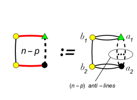
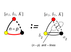
In order to not saturate the notation on the CHY-graphs, we introduce the definition given in Fig. 3.
Refer to caption
Refer to caption
Figure 3: Loop box and triangle definition .

3.1 One Loop Integrands Classification

As it is going to be checked in section 5, the terms 𝐃typea:bsubscriptsuperscript𝐃:𝑎𝑏limit-fromtype{\bf D}^{\,a:b}_{\rm type-\,*}’s have a physical meaning, as there is a relation between them and Feynman diagrams. Basically, the number of ωi:ja1:a2subscriptsuperscript𝜔:subscript𝑎1subscript𝑎2:𝑖𝑗\omega^{a_{1}:a_{2}}_{i:j}’s in

La1:a2=PTtree[1,2,,n]×𝐃typea1:a2[n,n1,,1]superscriptsubscript𝐿:subscript𝑎1subscript𝑎2subscriptPTtree12𝑛subscriptsuperscript𝐃:subscript𝑎1subscript𝑎2limit-fromtype𝑛𝑛11\mathcal{I}_{L}^{a_{1}:a_{2}}={\rm PT_{tree}}[1,2,\ldots,n]\times{\bf D}^{\,a_{1}:a_{2}}_{\rm type-\,*}[n,n-1,\ldots,1]

corresponds to the number of legs attached to the loop in the Feynman diagram, and the term in

Rb1:b2=PTtree[1,2,,n]×(σijωi:jb1:b2)superscriptsubscript𝑅:subscript𝑏1subscript𝑏2subscriptPTtree12𝑛subscript𝜎𝑖𝑗subscriptsuperscript𝜔:subscript𝑏1subscript𝑏2:𝑖𝑗\mathcal{I}_{R}^{b_{1}:b_{2}}={\rm PT_{tree}}[1,2,\ldots,n]\times\left(\sigma_{ij}\,\omega^{b_{1}:b_{2}}_{i:j}\right)

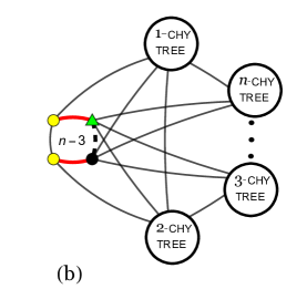
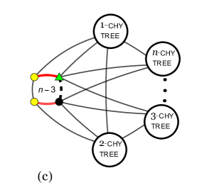
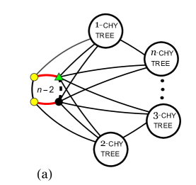
with a single ωi:jb1:b2subscriptsuperscript𝜔:subscript𝑏1subscript𝑏2:𝑖𝑗\omega^{b_{1}:b_{2}}_{i:j} will be in charge of its ordering. In fact, the CHY-integrand, La1:a2×Rb1:b2(a1,b1,b2,a2)2superscriptsubscript𝐿:subscript𝑎1subscript𝑎2superscriptsubscript𝑅:subscript𝑏1subscript𝑏2superscriptsubscript𝑎1subscript𝑏1subscript𝑏2subscript𝑎22\frac{\mathcal{I}_{L}^{a_{1}:a_{2}}\times\mathcal{I}_{R}^{b_{1}:b_{2}}}{(a_{1},b_{1},b_{2},a_{2})^{2}}, can be represented as a linear combination of the three CHY-graphs given in Fig. 4.
Refer to caption
Refer to caption
Refer to caption
Figure 4: Fundamental CHY-Integrands at one-loop.

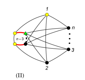
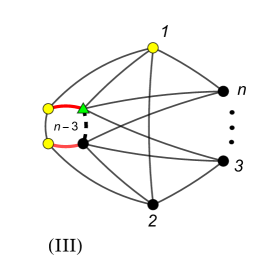
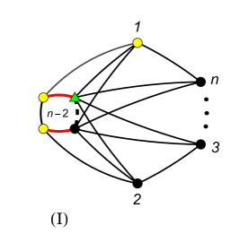
In particular, in Fig. 5 we consider the simplest cases.
Refer to caption
Refer to caption
Refer to caption
Figure 5: Simplest cases of CHY-graphs from Fig. 4.

In order to apply the ΛΛ\Lambda-algorithm to integrate the CHY-graphs in Fig. 5, we have fixed the punctures {σ1,σb1,σb2}subscript𝜎1subscript𝜎subscript𝑏1subscript𝜎subscript𝑏2\{\sigma_{1},\sigma_{b_{1}},\sigma_{b_{2}}\} by the PSL(2,)PSL2{\rm PSL}(2,\mathbb{C}) symmetry and the puncture {σa1}subscript𝜎subscript𝑎1\{\sigma_{a_{1}}\} by the scale symmetry Gomez:2016bmv . Clearly, we are using a different gauge than the one introduced in Gomez:2017lhy . This new gauge will allows us to work à la Feynman, i.e. each cut on the CHY-graph becomes a Feynman propagator, quadratic in momenta.

The CHY-graphs in Fig. 5 come from the following set of integrands

(I)I\displaystyle{\rm(I)} =PTtree[1,,n]𝐃type0a1:a2[n,,1]nω×PTtree[1,,n]σ12ω1:2b1:b2(a1,b1,b2,a2)2absentsubscriptPTtree1𝑛subscriptsuperscript𝐃:subscript𝑎1subscript𝑎2type0superscript𝑛1𝑛𝜔subscriptPTtree1𝑛subscript𝜎12subscriptsuperscript𝜔:subscript𝑏1subscript𝑏2:12superscriptsubscript𝑎1subscript𝑏1subscript𝑏2subscript𝑎22\displaystyle=\frac{{\rm PT}_{\rm tree}[1,\ldots,n]\,\mathbf{D}^{\,a_{1}:a_{2}}_{\rm type-0}[n,\ldots,1]^{n\omega}\times{\rm PT}_{\rm tree}[1,\ldots,n]\,\sigma_{12}\,\omega^{b_{1}:b_{2}}_{1:2}}{(a_{1},b_{1},b_{2},a_{2})^{2}}
=(n,n1,,1)×ω1:1a1:a2ω2:2a1:a2ωn:na1:a2×σ12ω1:2b1:b2(a1,b1,b2,a2)2×(1,2,,n)×(1,2,,n):=𝐈(I)CHY[1,,n]1:2+,absent𝑛𝑛11superscriptsubscript𝜔:11:subscript𝑎1subscript𝑎2superscriptsubscript𝜔:22:subscript𝑎1subscript𝑎2superscriptsubscript𝜔:𝑛𝑛:subscript𝑎1subscript𝑎2subscript𝜎12subscriptsuperscript𝜔:subscript𝑏1subscript𝑏2:12superscriptsubscript𝑎1subscript𝑏1subscript𝑏2subscript𝑎2212𝑛12𝑛assignsubscriptsuperscript𝐈CHYIsuperscript1𝑛:12\displaystyle=\frac{(n,n-1,\ldots,1)\times\omega_{1:1}^{a_{1}:a_{2}}\omega_{2:2}^{a_{1}:a_{2}}\cdots\omega_{n:n}^{a_{1}:a_{2}}\times\sigma_{12}\,\omega^{b_{1}:b_{2}}_{1:2}}{(a_{1},b_{1},b_{2},a_{2})^{2}\times(1,2,\ldots,n)\times(1,2,\ldots,n)}:=\mathbf{I}^{\rm CHY}_{{\rm(I)}}[1,\ldots,n]^{1:2}+\cdots,
(II)II\displaystyle{\rm(II)} =PTtree[1,,n]𝐃typeIa1:a2[n,,1](n1)ω×PTtree[1,,n]σ12ω1:2b1:b2(a1,b1,b2,a2)2absentsubscriptPTtree1𝑛subscriptsuperscript𝐃:subscript𝑎1subscript𝑎2typeIsuperscript𝑛1𝑛1𝜔subscriptPTtree1𝑛subscript𝜎12subscriptsuperscript𝜔:subscript𝑏1subscript𝑏2:12superscriptsubscript𝑎1subscript𝑏1subscript𝑏2subscript𝑎22\displaystyle=\frac{{\rm PT}_{\rm tree}[1,\ldots,n]\,\mathbf{D}^{\,a_{1}:a_{2}}_{\rm type-I}[n,\ldots,1]^{(n-1)\omega}\times{\rm PT}_{\rm tree}[1,\ldots,n]\,\sigma_{12}\,\omega^{b_{1}:b_{2}}_{1:2}}{(a_{1},b_{1},b_{2},a_{2})^{2}}
=+(1σ,nσ,3σ,2ω)a1:a2×ω3:3a1:a2ωn:na1:a2×σ12ω1:2b1:b2(a1,b1,b2,a2)2×(1,2,,n)×(1,2,,n):=𝐈(II)CHY[1,,n]1:2+,absentsuperscriptsuperscript1𝜎superscript𝑛𝜎superscript3𝜎superscript2𝜔:subscript𝑎1subscript𝑎2superscriptsubscript𝜔:33:subscript𝑎1subscript𝑎2superscriptsubscript𝜔:𝑛𝑛:subscript𝑎1subscript𝑎2subscript𝜎12subscriptsuperscript𝜔:subscript𝑏1subscript𝑏2:12superscriptsubscript𝑎1subscript𝑏1subscript𝑏2subscript𝑎2212𝑛12𝑛assignsubscriptsuperscript𝐈CHYIIsuperscript1𝑛:12\displaystyle=\cdots+\frac{(1^{\sigma},n^{\sigma}\ldots,3^{\sigma},2^{\omega})^{a_{1}:a_{2}}\times\omega_{3:3}^{a_{1}:a_{2}}\cdots\omega_{n:n}^{a_{1}:a_{2}}\times\sigma_{12}\,\omega^{b_{1}:b_{2}}_{1:2}}{(a_{1},b_{1},b_{2},a_{2})^{2}\times(1,2,\ldots,n)\times(1,2,\ldots,n)}:=\mathbf{I}^{\rm CHY}_{{\rm(II)}}[1,\ldots,n]^{1:2}+\cdots,
(III)III\displaystyle{\rm(III)} =PTtree[n,,1]𝐃typeIa1:a2[1,,n](n1)ω×PTtree[1,,n]σ12ω1:2b1:b2(a1,b1,b2,a2)2absentsubscriptPTtree𝑛1subscriptsuperscript𝐃:subscript𝑎1subscript𝑎2typeIsuperscript1𝑛𝑛1𝜔subscriptPTtree1𝑛subscript𝜎12subscriptsuperscript𝜔:subscript𝑏1subscript𝑏2:12superscriptsubscript𝑎1subscript𝑏1subscript𝑏2subscript𝑎22\displaystyle=\frac{{\rm PT}_{\rm tree}[n,\ldots,1]\,\mathbf{D}^{\,a_{1}:a_{2}}_{\rm type-I}[1,\ldots,n]^{(n-1)\omega}\times{\rm PT}_{\rm tree}[1,\ldots,n]\,\sigma_{12}\,\omega^{b_{1}:b_{2}}_{1:2}}{(a_{1},b_{1},b_{2},a_{2})^{2}}
=+(2σ,,nσ,1ω)a1:a2×ω3:3a1:a2ωn:na1:a2×σ12ω1:2b1:b2(a1,b1,b2,a2)2×(1,2,,n)×(n,n1,,1)+:=𝐈(III)CHY[1,,n]1:2+,absentsuperscriptsuperscript2𝜎superscript𝑛𝜎superscript1𝜔:subscript𝑎1subscript𝑎2superscriptsubscript𝜔:33:subscript𝑎1subscript𝑎2superscriptsubscript𝜔:𝑛𝑛:subscript𝑎1subscript𝑎2subscript𝜎12subscriptsuperscript𝜔:subscript𝑏1subscript𝑏2:12superscriptsubscript𝑎1subscript𝑏1subscript𝑏2subscript𝑎2212𝑛𝑛𝑛11assignsubscriptsuperscript𝐈CHYIIIsuperscript1𝑛:12\displaystyle=\cdots+\frac{(2^{\sigma},\ldots,n^{\sigma},1^{\omega})^{a_{1}:a_{2}}\times\omega_{3:3}^{a_{1}:a_{2}}\cdots\omega_{n:n}^{a_{1}:a_{2}}\times\sigma_{12}\,\omega^{b_{1}:b_{2}}_{1:2}}{(a_{1},b_{1},b_{2},a_{2})^{2}\times(1,2,\ldots,n)\times(n,n-1,\ldots,1)}+\cdots:=\mathbf{I}^{\rm CHY}_{{\rm(III)}}[1,\ldots,n]^{1:2}+\cdots\,,

where ellipsis stand for additional terms with the same structure666Sometimes, it is necessary to manipulate the integrand to obtain the CHY-graphs in Fig. 4. as those given in the graphs of Fig. 4.

Bearing in mind that the Λlimit-fromΛ\Lambda-algorithm is able to solve the CHY-graphs up to an overall sign the first point to tackle is how to fix this ambiguity777Notice that the overall sign can be fixed by the technique developed in Cardona:2016gon , where the anti-lines have been considered.. Let us consider the integrands, 𝐈(I)CHY[1,,n]1:2,𝐈(II)CHY[1,,n]1:2subscriptsuperscript𝐈CHYIsuperscript1𝑛:12subscriptsuperscript𝐈CHYIIsuperscript1𝑛:12\mathbf{I}^{\rm CHY}_{{\rm(I)}}[1,\ldots,n]^{1:2},\mathbf{I}^{\rm CHY}_{{\rm(II)}}[1,\ldots,n]^{1:2} and 𝐈(III)CHY[1,,n]1:2subscriptsuperscript𝐈CHYIIIsuperscript1𝑛:12\mathbf{I}^{\rm CHY}_{{\rm(III)}}[1,\ldots,n]^{1:2} above. Pulling out the common factors they become

𝐈(I)CHY[1,,n]1:2subscriptsuperscript𝐈CHYIsuperscript1𝑛:12\displaystyle\mathbf{I}^{\rm CHY}_{{\rm(I)}}[1,\ldots,n]^{1:2} =\displaystyle= (1)[(1)n+1σa1a2n2σa1b12σa2b22σb1b2×1i=1nσia1σia2×1σ1b1σ2b2σ23σn1],1delimited-[]superscript1𝑛1superscriptsubscript𝜎subscript𝑎1subscript𝑎2𝑛2superscriptsubscript𝜎subscript𝑎1subscript𝑏12superscriptsubscript𝜎subscript𝑎2subscript𝑏22subscript𝜎subscript𝑏1subscript𝑏21superscriptsubscriptproduct𝑖1𝑛subscript𝜎𝑖subscript𝑎1subscript𝜎𝑖subscript𝑎21subscript𝜎1subscript𝑏1subscript𝜎2subscript𝑏2subscript𝜎23subscript𝜎𝑛1\displaystyle(-1)\left[(-1)^{n+1}\,\,\frac{\sigma_{a_{1}a_{2}}^{n-2}}{\sigma_{a_{1}b_{1}}^{2}\sigma_{a_{2}b_{2}}^{2}\sigma_{b_{1}b_{2}}}\times\frac{1}{\prod_{i=1}^{n}\sigma_{ia_{1}}\sigma_{ia_{2}}}\times\frac{1}{\sigma_{1b_{1}}\sigma_{2b_{2}}\sigma_{23}\cdots\sigma_{n1}}\right], (22)
𝐈(II)CHY[1,,n]1:2subscriptsuperscript𝐈CHYIIsuperscript1𝑛:12\displaystyle\mathbf{I}^{\rm CHY}_{{\rm(II)}}[1,\ldots,n]^{1:2} =\displaystyle= (1)[(1)n+1σa1a2n3σa1b12σa2b22σb1b2×1σ1a2σ2a1i=3nσia1σia2×1σ1b1σ2b2(1,,n)],1delimited-[]superscript1𝑛1superscriptsubscript𝜎subscript𝑎1subscript𝑎2𝑛3superscriptsubscript𝜎subscript𝑎1subscript𝑏12superscriptsubscript𝜎subscript𝑎2subscript𝑏22subscript𝜎subscript𝑏1subscript𝑏21subscript𝜎1subscript𝑎2subscript𝜎2subscript𝑎1superscriptsubscriptproduct𝑖3𝑛subscript𝜎𝑖subscript𝑎1subscript𝜎𝑖subscript𝑎21subscript𝜎1subscript𝑏1subscript𝜎2subscript𝑏21𝑛\displaystyle(-1)\left[(-1)^{n+1}\,\,\frac{\sigma_{a_{1}a_{2}}^{n-3}}{\sigma_{a_{1}b_{1}}^{2}\sigma_{a_{2}b_{2}}^{2}\sigma_{b_{1}b_{2}}}\times\frac{1}{\sigma_{1a_{2}}\sigma_{2a_{1}}\prod_{i=3}^{n}\sigma_{ia_{1}}\sigma_{ia_{2}}}\times\frac{1}{\sigma_{1b_{1}}\sigma_{2b_{2}}(1,\ldots,n)}\right],
𝐈(III)CHY[1,,n]1:2subscriptsuperscript𝐈CHYIIIsuperscript1𝑛:12\displaystyle\mathbf{I}^{\rm CHY}_{{\rm(III)}}[1,\ldots,n]^{1:2} =\displaystyle= (1)[(1)n+1σa1a2n3σa1b12σa2b22σb1b2×1σ1a1σ2a2i=3nσia1σia2×1σ1b1σ2b2(1,,n)].1delimited-[]superscript1𝑛1superscriptsubscript𝜎subscript𝑎1subscript𝑎2𝑛3superscriptsubscript𝜎subscript𝑎1subscript𝑏12superscriptsubscript𝜎subscript𝑎2subscript𝑏22subscript𝜎subscript𝑏1subscript𝑏21subscript𝜎1subscript𝑎1subscript𝜎2subscript𝑎2superscriptsubscriptproduct𝑖3𝑛subscript𝜎𝑖subscript𝑎1subscript𝜎𝑖subscript𝑎21subscript𝜎1subscript𝑏1subscript𝜎2subscript𝑏21𝑛\displaystyle(-1)\left[(-1)^{n+1}\,\,\frac{\sigma_{a_{1}a_{2}}^{n-3}}{\sigma_{a_{1}b_{1}}^{2}\sigma_{a_{2}b_{2}}^{2}\sigma_{b_{1}b_{2}}}\times\frac{1}{\sigma_{1a_{1}}\sigma_{2a_{2}}\prod_{i=3}^{n}\sigma_{ia_{1}}\sigma_{ia_{2}}}\times\frac{1}{\sigma_{1b_{1}}\sigma_{2b_{2}}(1,\ldots,n)}\right].

We claim that the terms in the square brackets have a direct representation in terms of the CHY-graphs in Fig. 5.

In the following we make use of the Λlimit-fromΛ\Lambda-algorithm to perform the set of integrals 𝐈(I)CHY[1,,n]1:2subscriptsuperscript𝐈CHYIsuperscript1𝑛:12\mathbf{I}^{\rm CHY}_{{\rm(I)}}[1,\ldots,n]^{1:2}, 𝐈(II)CHY[1,,n]1:2subscriptsuperscript𝐈CHYIIsuperscript1𝑛:12\mathbf{I}^{\rm CHY}_{{\rm(II)}}[1,\ldots,n]^{1:2} and 𝐈(III)CHY[1,,n]1:2subscriptsuperscript𝐈CHYIIIsuperscript1𝑛:12\mathbf{I}^{\rm CHY}_{{\rm(III)}}[1,\ldots,n]^{1:2}. The conjectured overall sign inside the brackets in (22), (1)n+1superscript1𝑛1(-1)^{n+1}, is checked numerically afterwards888For the numerical checking we have fixed the punctures and scattering equations, {(σ1,E1),(σ2,E2),(σ3,E3)}subscript𝜎1subscript𝐸1subscript𝜎2subscript𝐸2subscript𝜎3subscript𝐸3\{(\sigma_{1},E_{1}),(\sigma_{2},E_{2}),(\sigma_{3},E_{3})\}, namely, the Faddeev-Popov determinant becomes (σ12σ23σ31)2superscriptsubscript𝜎12subscript𝜎23subscript𝜎312(\sigma_{12}\sigma_{23}\sigma_{31})^{2}. .

Proposition 1: There is an equality among the CHY-integral of (I)I{\rm(I)}, (22), and the one-loop n-point Feynman integrand

(I)CHY[1,,n]1:2:=12n+1𝑑Ωsa1b1𝑑μn+4tree𝐈(I)CHY[1,,n]1:2=[Uncaptioned image]assignsubscriptsuperscriptCHYIsuperscript1𝑛:121superscript2𝑛1differential-dΩsubscript𝑠subscript𝑎1subscript𝑏1differential-dsuperscriptsubscript𝜇𝑛4treesubscriptsuperscript𝐈CHYIsuperscript1𝑛:12[Uncaptioned image]\displaystyle\mathfrak{I}^{\rm CHY}_{\rm(I)}[1,\ldots,n]^{1:2}:=\frac{1}{2^{n+1}}\int d\Omega\,\,s_{a_{1}b_{1}}\int d\mu_{n+4}^{\rm tree}\,\,\mathbf{I}^{\rm CHY}_{{\rm(I)}}[1,\ldots,n]^{1:2}\,\,=\parbox[c]{100.00015pt}{\includegraphics[scale={0.2}]{feyn-p.pdf}}\,\, (23)

Proof: The result follows from a direct calculation,

(I)CHY[1,,n]1:2=12n+1𝑑Ω×sa1b1×𝑑μn+4tree𝐈(I)CHY[1,,n]1:2subscriptsuperscriptCHYIsuperscript1𝑛:121superscript2𝑛1differential-dΩsubscript𝑠subscript𝑎1subscript𝑏1differential-dsuperscriptsubscript𝜇𝑛4treesubscriptsuperscript𝐈CHYIsuperscript1𝑛:12\displaystyle\mathfrak{I}^{\rm CHY}_{\rm(I)}[1,\ldots,n]^{1:2}=\frac{1}{2^{n+1}}\int d\Omega\times s_{a_{1}b_{1}}\times\int d\mu_{n+4}^{\rm tree}\,\,\mathbf{I}^{\rm CHY}_{{\rm(I)}}[1,\ldots,n]^{1:2}
=(1)2n+1𝑑Ωsa1b1𝑑μn+4tree[(1)n+1σa1a2n2σa1b12σa2b22σb1b2×1i=1nσia1σia2×1σ1b1σ2b2σ23σn1]absent1superscript2𝑛1differential-dΩsubscript𝑠subscript𝑎1subscript𝑏1differential-dsuperscriptsubscript𝜇𝑛4treedelimited-[]superscript1𝑛1superscriptsubscript𝜎subscript𝑎1subscript𝑎2𝑛2superscriptsubscript𝜎subscript𝑎1subscript𝑏12superscriptsubscript𝜎subscript𝑎2subscript𝑏22subscript𝜎subscript𝑏1subscript𝑏21superscriptsubscriptproduct𝑖1𝑛subscript𝜎𝑖subscript𝑎1subscript𝜎𝑖subscript𝑎21subscript𝜎1subscript𝑏1subscript𝜎2subscript𝑏2subscript𝜎23subscript𝜎𝑛1\displaystyle=\frac{(-1)}{2^{n+1}}\int d\Omega\,s_{a_{1}b_{1}}\,\int d\mu_{n+4}^{\rm tree}\left[(-1)^{n+1}\,\,\frac{\sigma_{a_{1}a_{2}}^{n-2}}{\sigma_{a_{1}b_{1}}^{2}\sigma_{a_{2}b_{2}}^{2}\sigma_{b_{1}b_{2}}}\times\frac{1}{\prod_{i=1}^{n}\sigma_{ia_{1}}\sigma_{ia_{2}}}\times\frac{1}{\sigma_{1b_{1}}\sigma_{2b_{2}}\sigma_{23}\cdots\sigma_{n1}}\right]
=(1)2n+1𝑑Ωsa1b1𝑑μn+4tree[Uncaptioned image],absent1superscript2𝑛1differential-dΩsubscript𝑠subscript𝑎1subscript𝑏1differential-dsuperscriptsubscript𝜇𝑛4tree[Uncaptioned image]\displaystyle=\frac{(-1)}{2^{n+1}}\int d\Omega\,s_{a_{1}b_{1}}\,\int d\mu_{n+4}^{\rm tree}\parbox[c]{100.00015pt}{\includegraphics[scale={0.21}]{G-graph11.pdf}}\,\,, (24)

where in the last step we have mapped each element in the expression inside the bracket to the CHY-graph: The first factor is the box, namely the loop momenta sector, the second one is in charge of connecting the loop momenta to all the external points, and the third factor is the one that gives the ordering. With these identifications all the integrands of this type will look alike but with the external points permuted.

In order to compute the 𝑑μn+4treedifferential-dsuperscriptsubscript𝜇𝑛4tree\int d\mu_{n+4}^{\rm tree} integral within the ΛΛ\Lambda-algotithm Gomez:2016bmv , we introduce the “nearest neighbour” gauge fixing. One can show that it is necessary to perform a total of (n+1)limit-from𝑛1(n+1)-consecutive cuts, each one introducing a single propagator, like in the Feynman diagrams. For instance, using the Λlimit-fromΛ\Lambda-rules, there is only one non zero cut on the CHY-graph in (24), as it is shown on left graph in (25).

[Uncaptioned image]=1ka1b1×([Uncaptioned image]).[Uncaptioned image]1subscript𝑘subscript𝑎1subscript𝑏1[Uncaptioned image]\displaystyle\centering\parbox[c]{100.00015pt}{\includegraphics[scale={0.24}]{G-cut1.pdf}}=\,\,\,\frac{1}{k_{a_{1}b_{1}}}\times\left(\parbox[c]{120.00018pt}{\includegraphics[scale={0.24}]{G-cut2.pdf}}\right)\,\,.\@add@centering (25)

This first cut gives the factor 1ka1b11subscript𝑘subscript𝑎1subscript𝑏1\frac{1}{k_{a_{1}b_{1}}} and the resulting CHY-graph contains now a massive puncture with momentum, ka1+kb1subscript𝑘subscript𝑎1subscript𝑘subscript𝑏1k_{a_{1}}+k_{b_{1}}, which is connected with a double line to the puncture σ1subscript𝜎1\sigma_{1}. By scale symmetry we fix the nearest neighbour to σ1subscript𝜎1\sigma_{1} (next to its right), i.e. σnsubscript𝜎𝑛\sigma_{n} , such as it is shown on right graph in (25), see also Fig. 3.

The resulting CHY-graph in (25) contains also only one non zero cut, which we have dubbed cut-2. This cut is simple to compute and its result is given by

[Uncaptioned image]=1k234na2b2×([Uncaptioned image]),[Uncaptioned image]1subscript𝑘234𝑛subscript𝑎2subscript𝑏2[Uncaptioned image]\displaystyle\centering\parbox[c]{100.00015pt}{\includegraphics[scale={0.24}]{G-cut2.pdf}}\,\,=\,\,\,\frac{1}{k_{234\cdots na_{2}b_{2}}}\times\left(\parbox[c]{120.00018pt}{\includegraphics[scale={0.24}]{G-cut3.pdf}}\right),\@add@centering (26)

where clearly the resulting graph keeps the same form but with one less puncture. Iterating (n2)𝑛2(n-2) times this procedure we are led with

[Uncaptioned image]=1ka1b1×k234na2b2××k2a2b2×([Uncaptioned image])[Uncaptioned image]1subscript𝑘subscript𝑎1subscript𝑏1subscript𝑘234𝑛subscript𝑎2subscript𝑏2subscript𝑘2subscript𝑎2subscript𝑏2[Uncaptioned image]\displaystyle\centering\parbox[c]{90.00014pt}{\includegraphics[scale={0.24}]{G-cut1.pdf}}=\frac{1}{k_{a_{1}b_{1}}\times k_{234\cdots na_{2}b_{2}}\times\cdots\times k_{2a_{2}b_{2}}}\times\left(\parbox[c]{80.00012pt}{\includegraphics[scale={0.24}]{G-cutn.pdf}}\right)\@add@centering (27)

This final resulting graph has just one non-zero cut, as it is shown in (27), which we have called “cut-(n+1)” and its result by the Λlimit-fromΛ\Lambda-rules is 1ka2b21subscript𝑘subscript𝑎2subscript𝑏2\frac{1}{k_{a_{2}b_{2}}}.

Summarizing, so far we have proven the equality

𝑑μn+4tree[Uncaptioned image]=2n+1sa1b1×s1a1b1×s1na1b1××s1n(n1)3a1b1×sa2b2,differential-dsuperscriptsubscript𝜇𝑛4tree[Uncaptioned image]superscript2𝑛1subscript𝑠subscript𝑎1subscript𝑏1subscript𝑠1subscript𝑎1subscript𝑏1subscript𝑠1𝑛subscript𝑎1subscript𝑏1subscript𝑠1𝑛𝑛13subscript𝑎1subscript𝑏1subscript𝑠subscript𝑎2subscript𝑏2\displaystyle\int d\mu_{n+4}^{\rm tree}\parbox[c]{90.00014pt}{\includegraphics[scale={0.21}]{G-graph11.pdf}}=\frac{2^{n+1}}{s_{a_{1}b_{1}}\times s_{1a_{1}b_{1}}\times s_{1na_{1}b_{1}}\times\cdots\times s_{1n(n-1)\cdots 3a_{1}b_{1}}\times s_{a_{2}b_{2}}}\,\,,

where the momentum conservation condition, i=1nki+ka1+ka2+kb1+kb2=0superscriptsubscript𝑖1𝑛subscript𝑘𝑖subscript𝑘subscript𝑎1subscript𝑘subscript𝑎2subscript𝑘subscript𝑏1subscript𝑘subscript𝑏20\sum_{i=1}^{n}k_{i}+k_{a_{1}}+k_{a_{2}}+k_{b_{1}}+k_{b_{2}}=0, has been used.

Carrying out the last integration, 𝑑Ω×sa1b1differential-dΩsubscript𝑠subscript𝑎1subscript𝑏1\int d\Omega\times s_{a_{1}b_{1}}, we are left with the following expression

12n+1𝑑Ω×sa1b1×2n+1sa1b1×s1a1b1×s1na1b1××s1n(n1)3a1b1×sa2b21superscript2𝑛1differential-dΩsubscript𝑠subscript𝑎1subscript𝑏1superscript2𝑛1subscript𝑠subscript𝑎1subscript𝑏1subscript𝑠1subscript𝑎1subscript𝑏1subscript𝑠1𝑛subscript𝑎1subscript𝑏1subscript𝑠1𝑛𝑛13subscript𝑎1subscript𝑏1subscript𝑠subscript𝑎2subscript𝑏2\displaystyle\frac{1}{2^{n+1}}\int d\Omega\times s_{a_{1}b_{1}}\times\frac{2^{n+1}}{s_{a_{1}b_{1}}\times s_{1a_{1}b_{1}}\times s_{1na_{1}b_{1}}\times\cdots\times s_{1n(n-1)\cdots 3a_{1}b_{1}}\times s_{a_{2}b_{2}}}
=12(+k1)2(+k1+kn)2(+k1+kn+kn1)2(+i,i2nki)2=[Uncaptioned image],absent1superscript2superscriptsubscript𝑘12superscriptsubscript𝑘1subscript𝑘𝑛2superscriptsubscript𝑘1subscript𝑘𝑛subscript𝑘𝑛12superscriptsuperscriptsubscript𝑖𝑖2𝑛subscript𝑘𝑖2[Uncaptioned image]\displaystyle=\frac{1}{\ell^{2}(\ell+k_{1})^{2}(\ell+k_{1}+k_{n})^{2}(\ell+k_{1}+k_{n}+k_{n-1})^{2}\cdots(\ell+\sum_{i,i\neq 2}^{n}k_{i})^{2}}\,\,=\parbox[c]{90.00014pt}{\includegraphics[scale={0.2}]{feyn-p.pdf}}\,\,,

where we have finally identified the algebraic expression with the pictorical one-loop n-point Feynman integrand. This equality, which corresponds to our initial claim, has also been checked numerically. \quad\blacksquare

As a final remark for this first proposition, we can generalize the previous calculation to the case of attaching CHY tree-level graphs instead of points as in (24). Schematically it is

12N+1𝑑Ω×sa1b1𝑑μN+4tree[Uncaptioned image]=[Uncaptioned image],1superscript2𝑁1differential-dΩsubscript𝑠subscript𝑎1subscript𝑏1differential-dsuperscriptsubscript𝜇𝑁4tree[Uncaptioned image][Uncaptioned image]\displaystyle\frac{1}{2^{N+1}}\int d\Omega\times s_{a_{1}b_{1}}\int d\mu_{N+4}^{\rm tree}\parbox[c]{100.00015pt}{\includegraphics[scale={0.21}]{G-type_a.pdf}}=\parbox[c]{80.00012pt}{\includegraphics[scale={0.2}]{G-Fey-type_a.pdf}}\,\,, (28)

where N𝑁N is the total number of external particles. The gluing process to join the CHY tree-level graphs at the one-loop skeleton can be found in Gomez:2016cqb ; Cardona:2016wcr . These kind of graphs can be solved in the same fashion as we did for the n𝑛n-point case.

Proposition 2: The CHY-integral of (II)II{\rm(II)}, (22), identically vanishes.

(II)CHY[1,,n]1:2:=12n+1𝑑Ω×sa1b1×𝑑μn+4tree𝐈(II)CHY[1,,n]1:2=0.assignsubscriptsuperscriptCHYIIsuperscript1𝑛:121superscript2𝑛1differential-dΩsubscript𝑠subscript𝑎1subscript𝑏1differential-dsuperscriptsubscript𝜇𝑛4treesubscriptsuperscript𝐈CHYIIsuperscript1𝑛:120\displaystyle\mathfrak{I}^{\rm CHY}_{\rm(II)}[1,\ldots,n]^{1:2}:=\frac{1}{2^{n+1}}\int d\Omega\times s_{a_{1}b_{1}}\times\int d\mu_{n+4}^{\rm tree}\,\,\mathbf{I}^{\rm CHY}_{{\rm(II)}}[1,\ldots,n]^{1:2}=0\,. (29)

Proof: As in the previous case, the proof is straightforward, but a little tedious.

(II)CHY[1,,n]1:2=12n+1𝑑Ω×sa1b1×𝑑μn+4tree𝐈(II)CHY[1,,n]1:2subscriptsuperscriptCHYIIsuperscript1𝑛:121superscript2𝑛1differential-dΩsubscript𝑠subscript𝑎1subscript𝑏1differential-dsuperscriptsubscript𝜇𝑛4treesubscriptsuperscript𝐈CHYIIsuperscript1𝑛:12\displaystyle\mathfrak{I}^{\rm CHY}_{\rm(II)}[1,\ldots,n]^{1:2}=\frac{1}{2^{n+1}}\int d\Omega\times s_{a_{1}b_{1}}\times\int d\mu_{n+4}^{\rm tree}\,\,\mathbf{I}^{\rm CHY}_{{\rm(II)}}[1,\ldots,n]^{1:2}
=dΩ2n+1sa1b1𝑑μn+4tree[(1)n+1σa1a2n3σa1b12σa2b22σb1b2×1σ1a2σ2a1i=3nσia1σia2×1σ1b1σ2b2(1,,n)]absent𝑑Ωsuperscript2𝑛1subscript𝑠subscript𝑎1subscript𝑏1differential-dsuperscriptsubscript𝜇𝑛4treedelimited-[]superscript1𝑛1superscriptsubscript𝜎subscript𝑎1subscript𝑎2𝑛3superscriptsubscript𝜎subscript𝑎1subscript𝑏12superscriptsubscript𝜎subscript𝑎2subscript𝑏22subscript𝜎subscript𝑏1subscript𝑏21subscript𝜎1subscript𝑎2subscript𝜎2subscript𝑎1superscriptsubscriptproduct𝑖3𝑛subscript𝜎𝑖subscript𝑎1subscript𝜎𝑖subscript𝑎21subscript𝜎1subscript𝑏1subscript𝜎2subscript𝑏21𝑛\displaystyle=-\int\frac{d\Omega}{2^{n+1}}\,s_{a_{1}b_{1}}\,\int d\mu_{n+4}^{\rm tree}\left[(-1)^{n+1}\,\,\frac{\sigma_{a_{1}a_{2}}^{n-3}}{\sigma_{a_{1}b_{1}}^{2}\sigma_{a_{2}b_{2}}^{2}\sigma_{b_{1}b_{2}}}\times\frac{1}{\sigma_{1a_{2}}\sigma_{2a_{1}}\prod_{i=3}^{n}\sigma_{ia_{1}}\sigma_{ia_{2}}}\times\frac{1}{\sigma_{1b_{1}}\sigma_{2b_{2}}(1,\ldots,n)}\right]
=(1)2n+1𝑑Ωsa1b1𝑑μn+4tree[Uncaptioned image].absent1superscript2𝑛1differential-dΩsubscript𝑠subscript𝑎1subscript𝑏1differential-dsuperscriptsubscript𝜇𝑛4tree[Uncaptioned image]\displaystyle=\frac{(-1)}{2^{n+1}}\int d\Omega\,s_{a_{1}b_{1}}\,\int d\mu_{n+4}^{\rm tree}\parbox[c]{100.00015pt}{\includegraphics[scale={0.21}]{G-graph22.pdf}}\,\,. (30)

Applying the ΛΛ\Lambda-rules on the graph in (30) to compute the integral, 𝑑μn+4treedifferential-dsubscriptsuperscript𝜇tree𝑛4\int d\mu^{\rm tree}_{n+4}, one obtains that there is just one non-zero cut

[Uncaptioned image]=1ka1b1×([Uncaptioned image]).[Uncaptioned image]1subscript𝑘subscript𝑎1subscript𝑏1[Uncaptioned image]\displaystyle\centering\parbox[c]{103.00018pt}{\includegraphics[scale={0.24}]{i2_n-1_cut1.pdf}}=\,\,\frac{1}{k_{a_{1}b_{1}}}\times\left(\parbox[c]{120.00018pt}{\includegraphics[scale={0.24}]{i2_n-1_final.pdf}}\right)\,\,.\@add@centering (31)

Furthermore all possible cuts on the resulting CHY-graph in (31) are zero, therefore one can conclude that the integral, (II)CHY[1,,n]1:2subscriptsuperscriptCHYIIsuperscript1𝑛:12\mathfrak{I}^{\rm CHY}_{\rm(II)}[1,\ldots,n]^{1:2}, vanishes, i.e.

(II)CHY[1,,n]1:2=(1)2n+1dΩsa1b1dμn+4tree[Uncaptioned image]=0.\displaystyle\mathfrak{I}^{\rm CHY}_{\rm(II)}[1,\ldots,n]^{1:2}=\frac{(-1)}{2^{n+1}}\int d\Omega\,s_{a_{1}b_{1}}\,\int d\mu_{n+4}^{\rm tree}\parbox[c]{100.00015pt}{\includegraphics[scale={0.21}]{G-graph22.pdf}}=0\,\,.\quad\blacksquare (32)

This calculation can be generalized to the case of attaching CHY tree-level graphs instead of points. Schematically it is

𝑑Ωsa1b1𝑑μN+4tree[Uncaptioned image]=0,differential-dΩsubscript𝑠subscript𝑎1subscript𝑏1differential-dsuperscriptsubscript𝜇𝑁4tree[Uncaptioned image]0\displaystyle\int d\Omega\,s_{a_{1}b_{1}}\,\int d\mu_{N+4}^{\rm tree}\parbox[c]{100.00015pt}{\includegraphics[scale={0.21}]{Gen-I2.pdf}}=0\,\,, (33)

where N𝑁N is the total number of external particles. These type of graphs, with tree-level CHY-graphs attached, can be solved in a similar way as we did for the case in (32).

Proposition 3: There is a correspondence between the CHY-integral of (III)III{\rm(III)}, (22), and the one-loop n-point Feynman integrand

(III)CHY[1,,n]1:2:=12n+1𝑑Ωsa1b1𝑑μn+4tree𝐈(III)CHY[1,,n]1:2=(1)[Uncaptioned image]assignsubscriptsuperscriptCHYIIIsuperscript1𝑛:121superscript2𝑛1differential-dΩsubscript𝑠subscript𝑎1subscript𝑏1differential-dsuperscriptsubscript𝜇𝑛4treesubscriptsuperscript𝐈CHYIIIsuperscript1𝑛:121[Uncaptioned image]\displaystyle\mathfrak{I}^{\rm CHY}_{\rm(III)}[1,\ldots,n]^{1:2}:=\frac{1}{2^{n+1}}\int d\Omega\,\,s_{a_{1}b_{1}}\int d\mu_{n+4}^{\rm tree}\,\,\mathbf{I}^{\rm CHY}_{{\rm(III)}}[1,\ldots,n]^{1:2}=(-1)\parbox[c]{120.00018pt}{\includegraphics[scale={0.2}]{feyn-p.pdf}}\,\, (34)

Proof: The result follows from a direct calculation,

(III)CHY[1,,n]1:2=12n+1𝑑Ω×sa1b1×𝑑μn+4tree𝐈(III)CHY[1,,n]1:2subscriptsuperscriptCHYIIIsuperscript1𝑛:121superscript2𝑛1differential-dΩsubscript𝑠subscript𝑎1subscript𝑏1differential-dsuperscriptsubscript𝜇𝑛4treesubscriptsuperscript𝐈CHYIIIsuperscript1𝑛:12\displaystyle\mathfrak{I}^{\rm CHY}_{\rm(III)}[1,\ldots,n]^{1:2}=\frac{1}{2^{n+1}}\int d\Omega\times s_{a_{1}b_{1}}\times\int d\mu_{n+4}^{\rm tree}\,\,\mathbf{I}^{\rm CHY}_{{\rm(III)}}[1,\ldots,n]^{1:2}
=(1)2n+1𝑑Ωsa1b1𝑑μn+4tree[(1)n+1σa1a2n3σa1b12σa2b22σb1b2×1σ1a1σ2a2i=3nσia1σia2×1σ1b1σ2b2(1,,n)]absent1superscript2𝑛1differential-dΩsubscript𝑠subscript𝑎1subscript𝑏1differential-dsuperscriptsubscript𝜇𝑛4treedelimited-[]superscript1𝑛1superscriptsubscript𝜎subscript𝑎1subscript𝑎2𝑛3superscriptsubscript𝜎subscript𝑎1subscript𝑏12superscriptsubscript𝜎subscript𝑎2subscript𝑏22subscript𝜎subscript𝑏1subscript𝑏21subscript𝜎1subscript𝑎1subscript𝜎2subscript𝑎2superscriptsubscriptproduct𝑖3𝑛subscript𝜎𝑖subscript𝑎1subscript𝜎𝑖subscript𝑎21subscript𝜎1subscript𝑏1subscript𝜎2subscript𝑏21𝑛\displaystyle=\frac{(-1)}{2^{n+1}}\int d\Omega\,s_{a_{1}b_{1}}\,\int d\mu_{n+4}^{\rm tree}\left[(-1)^{n+1}\,\frac{\sigma_{a_{1}a_{2}}^{n-3}}{\sigma_{a_{1}b_{1}}^{2}\sigma_{a_{2}b_{2}}^{2}\sigma_{b_{1}b_{2}}}\times\frac{1}{\sigma_{1a_{1}}\sigma_{2a_{2}}\prod_{i=3}^{n}\sigma_{ia_{1}}\sigma_{ia_{2}}}\times\frac{1}{\sigma_{1b_{1}}\sigma_{2b_{2}}(1,\ldots,n)}\right]
=(1)2n+1𝑑Ωsa1b1𝑑μn+4tree[Uncaptioned image].absent1superscript2𝑛1differential-dΩsubscript𝑠subscript𝑎1subscript𝑏1differential-dsuperscriptsubscript𝜇𝑛4tree[Uncaptioned image]\displaystyle=\frac{(-1)}{2^{n+1}}\int d\Omega\,s_{a_{1}b_{1}}\,\int d\mu_{n+4}^{\rm tree}\parbox[c]{100.00015pt}{\includegraphics[scale={0.21}]{G-graph33.pdf}}\,\,. (35)

To compute this integral we use the previous results together with the cross-ratio identity

𝟙=σ12σa1a2σ1a2σ2a1+σ1a1σ2a2σ1a2σ2a1.double-struck-𝟙subscript𝜎12subscript𝜎subscript𝑎1subscript𝑎2subscript𝜎1subscript𝑎2subscript𝜎2subscript𝑎1subscript𝜎1subscript𝑎1subscript𝜎2subscript𝑎2subscript𝜎1subscript𝑎2subscript𝜎2subscript𝑎1\displaystyle\mathbb{1}=-\frac{\sigma_{12}\,\sigma_{a_{1}a_{2}}}{\sigma_{1a_{2}}\sigma_{2a_{1}}}+\frac{\sigma_{1a_{1}}\sigma_{2a_{2}}}{\sigma_{1a_{2}}\sigma_{2a_{1}}}\,. (36)

It is straightforward to check that by multiplying the CHY-integrand (or graph) in (35) times the above identity and using Proposition 2, the integral, (III)CHY[1,,n]1:2subscriptsuperscriptCHYIIIsuperscript1𝑛:12\mathfrak{I}^{\rm CHY}_{\rm(III)}[1,\ldots,n]^{1:2}, becomes

(III)CHY[1,,n]1:2subscriptsuperscriptCHYIIIsuperscript1𝑛:12\displaystyle\mathfrak{I}^{\rm CHY}_{\rm(III)}[1,\ldots,n]^{1:2} =12n+1𝑑Ω×sa1b1×𝑑μn+4tree𝐈(III)CHY[1,,n]1:2×𝟙absent1superscript2𝑛1differential-dΩsubscript𝑠subscript𝑎1subscript𝑏1differential-dsuperscriptsubscript𝜇𝑛4treesubscriptsuperscript𝐈CHYIIIsuperscript1𝑛:12double-struck-𝟙\displaystyle=\frac{1}{2^{n+1}}\int d\Omega\times s_{a_{1}b_{1}}\times\int d\mu_{n+4}^{\rm tree}\,\,\mathbf{I}^{\rm CHY}_{{\rm(III)}}[1,\ldots,n]^{1:2}\times\mathbb{1}
=(I)CHY[1,,n]1:2+(II)CHY[1,,n]1:2absentsubscriptsuperscriptCHYIsuperscript1𝑛:12subscriptsuperscriptCHYIIsuperscript1𝑛:12\displaystyle=-\mathfrak{I}^{\rm CHY}_{\rm(I)}[1,\ldots,n]^{1:2}+\mathfrak{I}^{\rm CHY}_{\rm(II)}[1,\ldots,n]^{1:2}
=(I)CHY[1,,n]1:2,absentsubscriptsuperscriptCHYIsuperscript1𝑛:12\displaystyle=-\mathfrak{I}^{\rm CHY}_{\rm(I)}[1,\ldots,n]^{1:2}\,, (37)

and consequently

12n+1𝑑Ω×sa1b1𝑑μn+4tree[Uncaptioned image]=(1)[Uncaptioned image]1superscript2𝑛1differential-dΩsubscript𝑠subscript𝑎1subscript𝑏1differential-dsuperscriptsubscript𝜇𝑛4tree[Uncaptioned image]1[Uncaptioned image]\displaystyle\frac{1}{2^{n+1}}\int d\Omega\times s_{a_{1}b_{1}}\int d\mu_{n+4}^{\rm tree}\parbox[c]{95.00014pt}{\includegraphics[scale={0.21}]{G-graph33.pdf}}=\,\,\,(-1)\parbox[c]{90.00014pt}{\includegraphics[scale={0.2}]{feyn-p.pdf}}\,\,\blacksquare (38)

This result can also be generalized for external CHY tree graphs. Schematically it is

12N+1𝑑Ω×sa1b1𝑑μN+4tree[Uncaptioned image]=(1)[Uncaptioned image],1superscript2𝑁1differential-dΩsubscript𝑠subscript𝑎1subscript𝑏1differential-dsuperscriptsubscript𝜇𝑁4tree[Uncaptioned image]1[Uncaptioned image]\displaystyle\frac{1}{2^{N+1}}\int d\Omega\times s_{a_{1}b_{1}}\int d\mu_{N+4}^{\rm tree}\parbox[c]{100.00015pt}{\includegraphics[scale={0.21}]{G-type_a33.pdf}}=\,\,\,(-1)\parbox[c]{90.00014pt}{\includegraphics[scale={0.2}]{G-Fey-type_a.pdf}}\,\,, (39)

where N𝑁N is the total number of external particles and again we can solve these type of CHY-graphs like we have done in the previous cases.

Now that we have a classification for the type of integrands that will appear in our calculations we can employ the results in the computation of the integrands for the Bi-adjoint Φ3superscriptΦ3\Phi^{3} scalar theory.

4 The bi-adjoint Φ3superscriptΦ3\Phi^{3} scalar theory

The scattering amplitudes at tree level for the massless bi-adjoint Φ3superscriptΦ3\Phi^{3} scalar theory are given by the elements Cachazo:2013iea

mntree[π|ρ]:=12n3𝑑μntreetCHY[π|ρ]assignsuperscriptsubscript𝑚𝑛treedelimited-[]conditional𝜋𝜌1superscript2𝑛3differential-dsuperscriptsubscript𝜇𝑛treesuperscriptsubscripttCHYdelimited-[]conditional𝜋𝜌\displaystyle m_{n}^{\rm tree}[\pi|\rho]:={1\over 2^{n-3}}\int\,\,d\mu_{n}^{\rm tree}\,\,\cal{I}_{\rm t}^{\rm CHY}[\pi|\rho] (40)

where

treeCHY[π|ρ]:=PTtree[π]×PTtree[ρ]assignsuperscriptsubscripttreeCHYdelimited-[]conditional𝜋𝜌subscriptPTtreedelimited-[]𝜋subscriptPTtreedelimited-[]𝜌\cal{I}_{\rm tree}^{\rm CHY}[\pi|\rho]:={\rm PT}_{\rm tree}[\pi]\times{\rm PT}_{\rm tree}[\rho] (41)

and the measure, dμntree𝑑superscriptsubscript𝜇𝑛treed\mu_{n}^{\rm tree}, is given in (17).

In Cachazo:2013iea , it was shown that the integral, mntree[π|ρ]superscriptsubscript𝑚𝑛treedelimited-[]conditional𝜋𝜌m_{n}^{\rm tree}[\pi|\rho], is composed by the sum over all the trivalent Feynman diagrams containing two planar embeddings, consistent with the π𝜋\pi (ρ𝜌\rho) ordering respectively999There are many techniques to compute mntree[π|ρ]superscriptsubscript𝑚𝑛treedelimited-[]conditional𝜋𝜌m_{n}^{\rm tree}[\pi|\rho], such as ones given in Gomez:2016cqb ; Chen:2017edo ; Cardona:2016gon ; Huang:2016zzb ; Cardona:2015ouc ; Kalousios:2015fya ; Mafra:2016ltu ; Cachazo:2013iea ; Baadsgaard:2015voa ; Cachazo:2015nwa ; Cardona:2015eba .. Specifically mntree[π|ρ]superscriptsubscript𝑚𝑛treedelimited-[]conditional𝜋𝜌m_{n}^{\rm tree}[\pi|\rho] reduces to the sum over all elements contained in the intersection among these two planar ordering. Schematically it can be written as Cachazo:2013iea

mntree[π|ρ]=(1)n3+nπ|ρmntree[π|π]mntree[ρ|ρ],superscriptsubscript𝑚𝑛treedelimited-[]conditional𝜋𝜌superscript1𝑛3subscript𝑛conditional𝜋𝜌superscriptsubscript𝑚𝑛treedelimited-[]conditional𝜋𝜋superscriptsubscript𝑚𝑛treedelimited-[]conditional𝜌𝜌\displaystyle m_{n}^{\rm tree}[\pi|\rho]=(-1)^{n-3+n_{\pi|\rho}}m_{n}^{\rm tree}[\pi|\pi]\cap m_{n}^{\rm tree}[\rho|\rho]\,, (42)

where nπ|ρsubscript𝑛conditional𝜋𝜌n_{\pi|\rho} is determined by the number of flips between two permutations π,ρ𝜋𝜌\pi,\rho Cachazo:2013iea . For example, let us consider the element, m4tree[1234|1243]superscriptsubscript𝑚4treedelimited-[]conditional12341243m_{4}^{\rm tree}[1234|1243], it reads

m4tree[1234|1243]=m4tree[1234|1234]m4tree[1243|1243]=[Uncaptioned image]=[Uncaptioned image]superscriptsubscript𝑚4treedelimited-[]conditional12341243superscriptsubscript𝑚4treedelimited-[]conditional12341234superscriptsubscript𝑚4treedelimited-[]conditional12431243[Uncaptioned image][Uncaptioned image]\displaystyle m_{4}^{\rm tree}[1234|1243]=m_{4}^{\rm tree}[1234|1234]\cap m_{4}^{\rm tree}[1243|1243]=\parbox[c]{100.00015pt}{\includegraphics[scale={0.38}]{intersection-eps-converted-to.pdf}}=\parbox[c]{60.00009pt}{\includegraphics[scale={0.41}]{intersectionR-eps-converted-to.pdf}} (43)

which is the right answer. In the previous example one can appreciate the advantage of (42), since the calculation for both orderings is exactly the same but with external legs permuted to the given ordering. Therefore, we only have to do the full calculation in the canonical ordering (i.e. (1,2,…,n)). This will prove extremely useful for the one-loop calculations.

4.1 Bi-adjoint Φ3superscriptΦ3\Phi^{3} at One-Loop

The CHY prescription to obtain the scattering integrands at one-loop, respecting the planar orderings (π𝜋\pi, ρ𝜌\rho), is given by the elements

mn1loop[π|ρ]=12n12𝑑μn+21loop1loopCHY[π|ρ],subscriptsuperscript𝑚1loop𝑛delimited-[]conditional𝜋𝜌1superscript2𝑛1superscript2differential-dsubscriptsuperscript𝜇1loop𝑛2superscriptsubscript1loopCHYdelimited-[]conditional𝜋𝜌\displaystyle m^{\rm 1-loop}_{n}[\pi|\rho]={1\over 2^{n-1}\,\,\ell^{2}}\int d\mu^{\rm 1-loop}_{n+2}\,\,\mathcal{I}_{\rm 1-loop}^{\rm CHY}[\pi|\rho], (44)

where

1loopCHY[π|ρ]:=1(+,)2×𝐏𝐓1loop+:[π]×𝐏𝐓1loop+:[ρ]assignsuperscriptsubscript1loopCHYdelimited-[]conditional𝜋𝜌1superscriptsuperscriptsuperscript2superscriptsubscript𝐏𝐓1loop:superscriptsuperscriptdelimited-[]𝜋superscriptsubscript𝐏𝐓1loop:superscriptsuperscriptdelimited-[]𝜌\mathcal{I}_{\rm 1-loop}^{\rm CHY}[\pi|\rho]:=\frac{1}{(\ell^{+},\ell^{-})^{2}}\times{\bf PT}_{\rm 1-loop}^{\,\ell^{+}:\ell^{-}}[\pi]\times{\bf PT}_{\rm 1-loop}^{\,\ell^{+}:\ell^{-}}[\rho] (45)

and the measure dμn+21loop𝑑subscriptsuperscript𝜇1loop𝑛2d\mu^{\rm 1-loop}_{n+2}

dμn+21loop:=assign𝑑subscriptsuperscript𝜇1loop𝑛2absent\displaystyle d\mu^{\rm 1-loop}_{n+2}:= dσ+dσa=1ndσaVol(PSL(2,))×(σ+σ1σ1+)a=2nEa1loop,𝑑subscript𝜎superscript𝑑subscript𝜎superscriptsuperscriptsubscriptproduct𝑎1𝑛𝑑subscript𝜎𝑎VolPSL2subscript𝜎superscriptsuperscriptsubscript𝜎superscript1subscript𝜎1superscriptsuperscriptsubscriptproduct𝑎2𝑛subscriptsuperscript𝐸1loop𝑎\displaystyle\frac{d\sigma_{\ell^{+}}d\sigma_{\ell^{-}}\prod_{a=1}^{n}d\sigma_{a}}{{\rm Vol}\,\,({\rm PSL}(2,\mathbb{C}))}\times\frac{(\sigma_{\ell^{+}\ell^{-}}\,\sigma_{\ell^{-}1}\,\sigma_{1\ell^{+}})}{\prod_{a=2}^{n}E^{\rm 1-loop}_{a}},
i=2nfixingPSL(2,)dσiEi1loop×(σ+σ1σ1+)2superscriptsuperscriptsubscriptproduct𝑖2𝑛fixingPSL2𝑑subscript𝜎𝑖subscriptsuperscript𝐸1loop𝑖superscriptsubscript𝜎superscriptsuperscriptsubscript𝜎superscript1subscript𝜎1superscript2{}^{\underrightarrow{\,\quad{\rm fixing\,\,PSL}(2,\mathbb{C})\,\quad}}\,\,\,\prod_{i=2}^{n}\frac{d\sigma_{i}}{E^{\rm 1-loop}_{i}}\times(\sigma_{\ell^{+}\ell^{-}}\,\sigma_{\ell^{-}1}\,\sigma_{1\ell^{+}})^{2} (46)

with

Ea1loop:=b=1bankakbσab+ka+σa++kaσa,a=1,,nformulae-sequenceassignsuperscriptsubscript𝐸𝑎1loopsubscriptsuperscript𝑛FRACOP𝑏1𝑏𝑎subscript𝑘𝑎subscript𝑘𝑏subscript𝜎𝑎𝑏subscript𝑘𝑎superscriptsubscript𝜎𝑎superscriptsubscript𝑘𝑎superscriptsubscript𝜎𝑎superscript𝑎1𝑛\displaystyle E_{a}^{\rm 1-loop}:=\sum^{n}_{b=1\atop b\neq a}\frac{k_{a}\cdot k_{b}}{\sigma_{ab}}+\frac{k_{a}\cdot\ell^{+}}{\sigma_{a\ell^{+}}}+\frac{k_{a}\cdot\ell^{-}}{\sigma_{a\ell^{-}}},\quad a=1,\ldots,n (47)
E±1loop:=b=1n±kbσ±b,(+)μ=()μ:=μ,20.formulae-sequenceformulae-sequenceassignsuperscriptsubscript𝐸superscriptplus-or-minus1loopsubscriptsuperscript𝑛𝑏1superscriptplus-or-minussubscript𝑘𝑏subscript𝜎superscriptplus-or-minus𝑏superscriptsuperscript𝜇superscriptsuperscript𝜇assignsuperscript𝜇superscript20\displaystyle E_{\ell^{\pm}}^{\rm 1-loop}:=\sum^{n}_{b=1}\frac{\ell^{\pm}\cdot k_{b}}{\sigma_{\ell^{\pm}b}},\qquad(\ell^{+})^{\mu}=-(\ell^{-})^{\mu}:=\ell^{\mu},\quad\ell^{2}\neq 0.

where, without loss of generality, we have fixed {σ+,σ,σ1}subscript𝜎superscriptsubscript𝜎superscriptsubscript𝜎1\{\sigma_{\ell^{+}},\sigma_{\ell^{-}},\sigma_{1}\} and {E+1loop,E1loop,E11loop}subscriptsuperscript𝐸1loopsuperscriptsubscriptsuperscript𝐸1loopsuperscriptsubscriptsuperscript𝐸1loop1\{E^{\rm 1-loop}_{\ell^{+}},E^{\rm 1-loop}_{\ell^{-}},E^{\rm 1-loop}_{1}\}.

As it has been shown in Geyer:2015jch ; He:2015yua ; Baadsgaard:2015hia , the CHY-integral in (44) reproduces the linear propagators in the internal loop momentum μsuperscript𝜇\ell^{\mu}, i.e. in the Q-cut representation Baadsgaard:2015twa ; Huang:2015cwh ; Feng:2016msc . Therefore, as it is very well known, these results match with the traditional Feynman propagators just after using the partial fraction identity and performing a shift in the loop momentum.

4.2 A New Proposal

In this section we propose a new CHY prescription for the S-matrix at one-loop of the bi-adjoint Φ3superscriptΦ3\Phi^{3} scalar theory, that takes into account the planar orderings. In this proposal we will be able reproduce directly the quadratic propagators, in the same way as the traditional Feynman approach.

Borrowing the line of reasoning in Gomez:2017lhy and the prescription (44) we arrive at:

Definition: The partial amplitude 𝔐n1loop[π|ρ]superscriptsubscript𝔐𝑛1loopdelimited-[]conditional𝜋𝜌\mathfrak{M}_{n}^{\rm 1-loop}[\pi|\rho] is given as

𝔐n1loop[π|ρ]:=12n+1𝑑Ω×(ka1+kb1)2×𝑑μn+4tree𝐈1loopCHY[π|ρ],assignsuperscriptsubscript𝔐𝑛1loopdelimited-[]conditional𝜋𝜌1superscript2𝑛1differential-dΩsuperscriptsubscript𝑘subscript𝑎1subscript𝑘subscript𝑏12differential-dsuperscriptsubscript𝜇𝑛4treesuperscriptsubscript𝐈1loopCHYdelimited-[]conditional𝜋𝜌\displaystyle\mathfrak{M}_{n}^{\rm 1-loop}[\pi|\rho]:={1\over 2^{n+1}}\int d\Omega\times(k_{a_{1}}+k_{b_{1}})^{2}\times\int d\mu_{n+4}^{\rm tree}\,\,\mathbf{I}_{\rm 1-loop}^{\rm CHY}[\pi|\rho], (48)

with

𝐈1loopCHY[π|ρ]:=𝐏𝐓1loopa1:a2[π]×1(a1,b1,b2,a2)2×𝐏𝐓1loopb1:b2[ρ].assignsuperscriptsubscript𝐈1loopCHYdelimited-[]conditional𝜋𝜌subscriptsuperscript𝐏𝐓:subscript𝑎1subscript𝑎21loopdelimited-[]𝜋1superscriptsubscript𝑎1subscript𝑏1subscript𝑏2subscript𝑎22subscriptsuperscript𝐏𝐓:subscript𝑏1subscript𝑏21loopdelimited-[]𝜌\mathbf{I}_{\rm 1-loop}^{\rm CHY}[\pi|\rho]:={\bf PT}^{\,a_{1}:a_{2}}_{\rm 1-loop}[\pi]\times\frac{1}{(a_{1},b_{1},b_{2},a_{2})^{2}}\times{\bf PT}^{\,b_{1}:b_{2}}_{\rm 1-loop}[\rho]. (49)

We conjecture that the amplitude, 𝔐n1loop[π|ρ]superscriptsubscript𝔐𝑛1loopdelimited-[]conditional𝜋𝜌\mathfrak{M}_{n}^{\rm 1-loop}[\pi|\rho], reproduces the integrands of the S-matrix elements at one-loop for the Φ3superscriptΦ3\Phi^{3} bi-adjoint massless theory. We are going to present several examples in order to support this statement.

Notice that despite the similarity among the prescriptions (44) and (48), there are significant differences between them: i) The total number of punctures do not match, namely in (44) there are n+2𝑛2n+2 punctures, out of which two are massive, while in (48) there are n+4𝑛4n+4 massless punctures. ii) The scattering equations are neither the same, although in Cachazo:2015aol it was shown that the massive scattering equations in (47) can be obtained from (18) after dimensional reduction. Additionally, iii) the final outcomes are different, as it is going to be shown later, (44) produces linear propagators in μsuperscript𝜇\ell^{\mu}, while (48) is able to reproduce the quadratic propagators as the traditional Feynman approach.

After some manipulations 𝐈1loopCHY[π|ρ]superscriptsubscript𝐈1loopCHYdelimited-[]conditional𝜋𝜌\mathbf{I}_{\rm 1-loop}^{\rm CHY}[\pi|\rho] in (49) becomes

𝐈1loopCHY[π|ρ]:=𝐏𝐓1loopa1:a2[π]×1(a1,b1,b2,a2)2×𝐏𝐓1loopb1:b2[ρ]assignsuperscriptsubscript𝐈1loopCHYdelimited-[]conditional𝜋𝜌subscriptsuperscript𝐏𝐓:subscript𝑎1subscript𝑎21loopdelimited-[]𝜋1superscriptsubscript𝑎1subscript𝑏1subscript𝑏2subscript𝑎22subscriptsuperscript𝐏𝐓:subscript𝑏1subscript𝑏21loopdelimited-[]𝜌\displaystyle\mathbf{I}_{\rm 1-loop}^{\rm CHY}[\pi|\rho]:={\bf PT}^{\,a_{1}:a_{2}}_{\rm 1-loop}[\pi]\times\frac{1}{(a_{1},b_{1},b_{2},a_{2})^{2}}\times{\bf PT}^{\,b_{1}:b_{2}}_{\rm 1-loop}[\rho]
=αcyc(π)βcyc(ρ)PTtree(α1,,αn,a1,b1,b2,a2)×PTtree(β1,,βn,b1,a1,a2,b2).absentsubscript𝛼cyc𝜋subscript𝛽cyc𝜌subscriptPTtreesubscript𝛼1subscript𝛼𝑛subscript𝑎1subscript𝑏1subscript𝑏2subscript𝑎2subscriptPTtreesubscript𝛽1subscript𝛽𝑛subscript𝑏1subscript𝑎1subscript𝑎2subscript𝑏2\displaystyle=\sum_{\alpha\in\rm cyc(\pi)}\sum_{\beta\in\rm cyc(\rho)}{\rm PT_{tree}}(\alpha_{1},\ldots,\alpha_{n},a_{1},b_{1},b_{2},a_{2})\times{\rm PT_{tree}}(\beta_{1},\ldots,\beta_{n},b_{1},a_{1},a_{2},b_{2}). (50)

As a consequence the integral, 𝑑μn+4tree𝐈1loopCHY[π|ρ]differential-dsuperscriptsubscript𝜇𝑛4treesuperscriptsubscript𝐈1loopCHYdelimited-[]conditional𝜋𝜌\int d\mu_{n+4}^{\rm tree}\,\mathbf{I}_{\rm 1-loop}^{\rm CHY}[\pi|\rho], is just a sum over trivalent tree level planar Feynman diagrams. However, this is not a very efficient and useful way to proceed because there is a large number of singular Feynman diagrams that do not contribute to the partial Amplitude, i.e. these diagrams must cancel out among them.

For example, consider the CHY-integrand

𝐈1loopCHY[1,2,3|1,2,3]=PTtree(1,2,3,a1,b1,b2,a2)×PTtree(1,2,3,b1,a1,a2,b2)+superscriptsubscript𝐈1loopCHY12conditional3123subscriptPTtree123subscript𝑎1subscript𝑏1subscript𝑏2subscript𝑎2subscriptPTtree123subscript𝑏1subscript𝑎1subscript𝑎2subscript𝑏2\mathbf{I}_{\rm 1-loop}^{\rm CHY}[1,2,3|1,2,3]={\rm PT_{tree}}(1,2,3,a_{1},b_{1},b_{2},a_{2})\times{\rm PT_{tree}}(1,2,3,b_{1},a_{1},a_{2},b_{2})+\cdots (51)

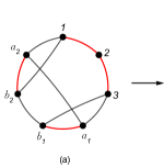
where ellipsis stand for terms obtained under cyclic permutations. The CHY-graph for the first term of the expansion in (51) is represented on the left hand side of Fig. 6.
Refer to caption
Refer to caption
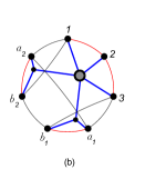
Figure 6: (a) CHY-graph for the first term in (51). (b) All trivalent Feynman diagrams associated to the CHY-graph (The grey circle means the sum over all possible trivalent vertices.).

The integral

𝑑μ3+4treePTtree(1,2,3,a1,b1,b2,a2)×PTtree(1,2,3,b1,a1,a2,b2),differential-dsuperscriptsubscript𝜇34treesubscriptPTtree123subscript𝑎1subscript𝑏1subscript𝑏2subscript𝑎2subscriptPTtree123subscript𝑏1subscript𝑎1subscript𝑎2subscript𝑏2\int d\mu_{3+4}^{\rm tree}\,{\rm PT_{tree}}(1,2,3,a_{1},b_{1},b_{2},a_{2})\times{\rm PT_{tree}}(1,2,3,b_{1},a_{1},a_{2},b_{2})\,,

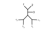
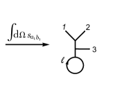
contains the sum over all possible trivalent planar Feynman diagrams, Cachazo:2013iea ; Mafra:2016ltu ; Baadsgaard:2015voa ; Gomez:2016bmv , that have been depicted with a grey circle and blue lines in Fig. 6(b). In particular, in Fig. 7(a) we give one example. Clearly, by performing the 𝑑Ωsa1b1differential-dΩsubscript𝑠subscript𝑎1subscript𝑏1\int d\Omega\,s_{a_{1}b_{1}} integral of this diagram, one obtains a tadpole, such as it is shown in Fig. 7(b). This singular diagram must not contribute to the amplitude and therefore it cancels out with another one which comes from the next contributions. This kind of analysis is tedious since the number of tree level diagrams in (4.2) is large.
Refer to caption
Refer to caption
Figure 7: One of all possible Feynman diagrams given in Fig. 6(b). Resulting tadpole after making the forward limit, i.e. by integrating 𝑑Ω(ka1+kb1)2differential-dΩsuperscriptsubscript𝑘subscript𝑎1subscript𝑘subscript𝑏12\int d\Omega\,(k_{a_{1}}+k_{b_{1}})^{2}.

In order to handle this group of cancelling diagrams without going through the detailed analysis described above, we shall rely on the findings of sections 2 and 3 to classify the Feynman diagrams at one-loop from the CHY approach. In the next section we are going to show several examples where this new technology is applied and the conjecture over 𝔐n1loop[π|ρ]superscriptsubscript𝔐𝑛1loopdelimited-[]conditional𝜋𝜌\mathfrak{M}_{n}^{\rm 1-loop}[\pi|\rho] will be checked.

Finally, note that the method used in He:2015yua ; Baadsgaard:2015hia could be applied here with a small variation: the off-shell momenta, μsuperscript𝜇\ell^{\mu} and μsuperscript𝜇-\ell^{\mu}, are split into two on-shell momenta, (ka1μ,kb1μ)superscriptsubscript𝑘subscript𝑎1𝜇superscriptsubscript𝑘subscript𝑏1𝜇(k_{a_{1}}^{\mu},k_{b_{1}}^{\mu}) and (ka2μ,kb2μ)superscriptsubscript𝑘subscript𝑎2𝜇superscriptsubscript𝑘subscript𝑏2𝜇(k_{a_{2}}^{\mu},k_{b_{2}}^{\mu}), as is shown in Fig. 6.

5 Examples

In the following section we will use all the previous results to calculate the particular cases n=3𝑛3n=3 and n=4𝑛4n=4. Since n=3𝑛3n=3 is simpler, it contains only two possible orderings, we will show all the contributions by direct calculation of the integrands in (13).

Before giving the examples, it is useful to introduce the following notation

[Uncaptioned image]:=[Uncaptioned image]+[Uncaptioned image]++[Uncaptioned image].assign[Uncaptioned image][Uncaptioned image][Uncaptioned image][Uncaptioned image]\displaystyle\parbox[c]{80.00012pt}{\includegraphics[scale={0.18}]{fey-1loop-T.pdf}}:=\parbox[c]{80.00012pt}{\includegraphics[scale={0.18}]{fey-1loop-01.pdf}}+\parbox[c]{80.00012pt}{\includegraphics[scale={0.18}]{fey-1loop-02.pdf}}+\cdots+\parbox[c]{100.00015pt}{\includegraphics[scale={0.18}]{fey-1loop-n.pdf}}. (52)

5.1 Three-point

In this case there are just two partial amplitudes, one coming from 𝔐31loop[1,2,3|1,2,3]superscriptsubscript𝔐31loop12conditional3123\mathfrak{M}_{3}^{\rm 1-loop}[1,2,3|1,2,3] and another from 𝔐31loop[1,2,3|3,2,1]superscriptsubscript𝔐31loop12conditional3321\mathfrak{M}_{3}^{\rm 1-loop}[1,2,3|3,2,1]. In addition, as inferred from (13), we have two expressions for 𝐏𝐓1loopa1:a2[1,2,3]subscriptsuperscript𝐏𝐓:subscript𝑎1subscript𝑎21loop123{\bf PT}^{\,a_{1}:a_{2}}_{\rm 1-loop}[1,2,3], one written in terms of the 𝐃typea:bsubscriptsuperscript𝐃:𝑎𝑏limit-fromtype{\bf D}^{\,a:b}_{\rm type-\,*}’s from the ordering (1,2,3), and the other in terms of the ordering (3,2,1). In the following we disentangle each of them.

5.1.1 Obtaining 𝔐31loop[1,2,3|1,2,3]superscriptsubscript𝔐31loop12conditional3123\mathfrak{M}_{3}^{\rm 1-loop}[1,2,3|1,2,3]

Let us start with the first CHY-integrand

𝐈1loopCHY[1,2,3|1,2,3]superscriptsubscript𝐈1loopCHY12conditional3123\displaystyle\mathbf{I}_{\rm 1-loop}^{\rm CHY}[1,2,3|1,2,3] =\displaystyle= PTtree[1,2,3]×PTtree[1,2,3](a1,b1,b2,a2)2×\displaystyle\frac{{\rm PT}_{\rm tree}[1,2,3]\times{\rm PT}_{\rm tree}[1,2,3]}{(a_{1},b_{1},b_{2},a_{2})^{2}}\times (53)
[ 2𝐃type0a1:a2[1,2,3]3ω+𝐃typeIa1:a2[1,2,3]2ω]×[σ12ω1:2b1:b2+σ23ω2:3b1:b2+σ31ω3:1b1:b2]delimited-[]2subscriptsuperscript𝐃:subscript𝑎1subscript𝑎2type0superscript1233𝜔subscriptsuperscript𝐃:subscript𝑎1subscript𝑎2typeIsuperscript1232𝜔delimited-[]subscript𝜎12subscriptsuperscript𝜔:subscript𝑏1subscript𝑏2:12subscript𝜎23subscriptsuperscript𝜔:subscript𝑏1subscript𝑏2:23subscript𝜎31subscriptsuperscript𝜔:subscript𝑏1subscript𝑏2:31\displaystyle\left[\,2\mathbf{D}^{\,a_{1}:a_{2}}_{\rm type-0}[1,2,3]^{3\omega}+\mathbf{D}^{\,a_{1}:a_{2}}_{\rm type-I}[1,2,3]^{2\omega}\right]\times\left[\sigma_{12}\,\omega^{b_{1}:b_{2}}_{1:2}+\sigma_{23}\,\omega^{b_{1}:b_{2}}_{2:3}+\sigma_{31}\omega^{b_{1}:b_{2}}_{3:1}\right]
=\displaystyle= [ 2𝐈(I)CHY[1,2,3]1:2+𝐈(III)CHY[1,2,3]1:2+𝐈(I)CHY[1,(2,3)]1:2+𝐈(I)CHY[(3,1),2]1:2\displaystyle-\left[\,2\mathbf{I}^{\rm CHY}_{\rm(I)}[1,2,3]^{1:2}+\mathbf{I}^{\rm CHY}_{\rm(III)}[1,2,3]^{1:2}+\mathbf{I}^{\rm CHY}_{\rm(I)}[1,(2,3)]^{1:2}+\mathbf{I}^{\rm CHY}_{\rm(I)}[(3,1),2]^{1:2}\right.
+cyc(1,2,3)]\displaystyle\left.\quad+{\rm cyc(1,2,3)}\right]

where we have introduced the shorthand notation

𝐈(I)CHY[i,(j,k)]i:jsubscriptsuperscript𝐈CHYIsuperscript𝑖𝑗𝑘:𝑖𝑗\displaystyle\mathbf{I}^{\rm CHY}_{{\rm(I)}}[i,(j,k)]^{i:j} :=(1)[(1)×1σa1b12σa2b22σb1b2×1σia1σia2×σja1σka2×1σib1σjb2σki×(j,k)],assignabsent1delimited-[]11superscriptsubscript𝜎subscript𝑎1subscript𝑏12superscriptsubscript𝜎subscript𝑎2subscript𝑏22subscript𝜎subscript𝑏1subscript𝑏21subscript𝜎𝑖subscript𝑎1subscript𝜎𝑖subscript𝑎2subscript𝜎𝑗subscript𝑎1subscript𝜎𝑘subscript𝑎21subscript𝜎𝑖subscript𝑏1subscript𝜎𝑗subscript𝑏2subscript𝜎𝑘𝑖𝑗𝑘\displaystyle:=(-1)\left[(-1)\times\frac{1}{\sigma_{a_{1}b_{1}}^{2}\sigma_{a_{2}b_{2}}^{2}\sigma_{b_{1}b_{2}}}\times\frac{1}{\sigma_{ia_{1}}\sigma_{ia_{2}}\times\sigma_{ja_{1}}\sigma_{ka_{2}}}\times\frac{1}{\sigma_{ib_{1}}\sigma_{jb_{2}}\sigma_{ki}\times(j,k)}\right],
𝐈(I)CHY[(k,i),j]i:jsubscriptsuperscript𝐈CHYIsuperscript𝑘𝑖𝑗:𝑖𝑗\displaystyle\mathbf{I}^{\rm CHY}_{{\rm(I)}}[(k,i),j]^{i:j} :=(1)[(1)×1σa1b12σa2b22σb1b2×1σka1σia2×σja1σja2×1σib1σjb2σjk×(k,i)].assignabsent1delimited-[]11superscriptsubscript𝜎subscript𝑎1subscript𝑏12superscriptsubscript𝜎subscript𝑎2subscript𝑏22subscript𝜎subscript𝑏1subscript𝑏21subscript𝜎𝑘subscript𝑎1subscript𝜎𝑖subscript𝑎2subscript𝜎𝑗subscript𝑎1subscript𝜎𝑗subscript𝑎21subscript𝜎𝑖subscript𝑏1subscript𝜎𝑗subscript𝑏2subscript𝜎𝑗𝑘𝑘𝑖\displaystyle:=(-1)\left[(-1)\times\frac{1}{\sigma_{a_{1}b_{1}}^{2}\sigma_{a_{2}b_{2}}^{2}\sigma_{b_{1}b_{2}}}\times\frac{1}{\sigma_{ka_{1}}\sigma_{ia_{2}}\times\sigma_{ja_{1}}\sigma_{ja_{2}}}\times\frac{1}{\sigma_{ib_{1}}\sigma_{jb_{2}}\sigma_{jk}\times(k,i)}\right].

In terms of the CHY-graphs one has

𝔐31loop[1,2,3|1,2,3]=124dΩ×sa1b1×\displaystyle\mathfrak{M}_{3}^{\rm 1-loop}[1,2,3|1,2,3]=\frac{1}{2^{4}}\int d\Omega\times s_{a_{1}b_{1}}\times (54)
𝑑μ3+4tree{2[Uncaptioned image]+[Uncaptioned image]+[Uncaptioned image]+[Uncaptioned image]+cyc(1,2,3)}.differential-dsuperscriptsubscript𝜇34tree2[Uncaptioned image][Uncaptioned image][Uncaptioned image][Uncaptioned image]cyc123\displaystyle\int d\mu_{3+4}^{\rm tree}\left\{2\parbox[c]{80.00012pt}{\includegraphics[scale={0.18}]{1-l_3-p_c1.pdf}}\,+\parbox[c]{80.00012pt}{\includegraphics[scale={0.18}]{1-l_3-p_c2.pdf}}\,+\parbox[c]{70.0001pt}{\includegraphics[scale={0.18}]{1-l_3-p_c3.pdf}}\,+\parbox[c]{80.00012pt}{\includegraphics[scale={0.18}]{1-l_3-p_c4.pdf}}+{\rm cyc(1,2,3)}\,\right\}.

That can be simplified further using (3.1)

𝔐31loop[1,2,3|1,2,3]=124dΩ×sa1b1×\displaystyle\mathfrak{M}_{3}^{\rm 1-loop}[1,2,3|1,2,3]=\frac{1}{2^{4}}\int d\Omega\times s_{a_{1}b_{1}}\times (55)
𝑑μ3+4tree{[Uncaptioned image]+[Uncaptioned image]+[Uncaptioned image]+cyc(1,2,3)}.differential-dsuperscriptsubscript𝜇34tree[Uncaptioned image][Uncaptioned image][Uncaptioned image]cyc123\displaystyle\int d\mu_{3+4}^{\rm tree}\left\{\parbox[c]{80.00012pt}{\includegraphics[scale={0.18}]{1-l_3-p_c1.pdf}}\,+\parbox[c]{70.0001pt}{\includegraphics[scale={0.18}]{1-l_3-p_c3.pdf}}\,+\parbox[c]{80.00012pt}{\includegraphics[scale={0.18}]{1-l_3-p_c4.pdf}}+{\rm cyc(1,2,3)}\,\right\}.

From the general result in section 3.1 the first integral reduces to

124𝑑Ωsa1b1𝑑μ3+4tree{[Uncaptioned image]+cyc(1,2,3)}=[Uncaptioned image],1superscript24differential-dΩsubscript𝑠subscript𝑎1subscript𝑏1differential-dsuperscriptsubscript𝜇34tree[Uncaptioned image]cyc123[Uncaptioned image]\displaystyle\frac{1}{2^{4}}\int d\Omega\,s_{a_{1}b_{1}}\int d\mu_{3+4}^{\rm tree}\left\{\parbox[c]{80.00012pt}{\includegraphics[scale={0.18}]{1-l_3-p_c1.pdf}}+{\rm cyc}(1,2,3)\right\}=\parbox[c]{100.00015pt}{\includegraphics[scale={0.23}]{fey-3pts-firstC.pdf}}\,, (56)

while the rest of terms can be cast in the general form depicted in Fig. 4(a), and their computations is totally similar to the one presented in section 3.1

124×sa1b1×𝑑μ3+4tree[Uncaptioned image]=1s23×1(ka2+kb2)2(k1+ka1+kb1)2,1superscript24subscript𝑠subscript𝑎1subscript𝑏1differential-dsuperscriptsubscript𝜇34tree[Uncaptioned image]1subscript𝑠231superscriptsubscript𝑘subscript𝑎2subscript𝑘subscript𝑏22superscriptsubscript𝑘1subscript𝑘subscript𝑎1subscript𝑘subscript𝑏12\displaystyle\frac{1}{2^{4}}\times s_{a_{1}b_{1}}\times\int d\mu_{3+4}^{\rm tree}\parbox[c]{70.0001pt}{\includegraphics[scale={0.18}]{1-l_3-p_c3.pdf}}=\frac{1}{s_{23}}\times\frac{1}{(k_{a_{2}}+k_{b_{2}})^{2}\,(k_{1}+k_{a_{1}}+k_{b_{1}})^{2}}, (57)
124×sa1b1×𝑑μ3+4tree[Uncaptioned image]=1s13×1(ka2+kb2)2(k1+k3+ka1+kb1)2.1superscript24subscript𝑠subscript𝑎1subscript𝑏1differential-dsuperscriptsubscript𝜇34tree[Uncaptioned image]1subscript𝑠131superscriptsubscript𝑘subscript𝑎2subscript𝑘subscript𝑏22superscriptsubscript𝑘1subscript𝑘3subscript𝑘subscript𝑎1subscript𝑘subscript𝑏12\displaystyle\frac{1}{2^{4}}\times s_{a_{1}b_{1}}\times\int d\mu_{3+4}^{\rm tree}\parbox[c]{70.0001pt}{\includegraphics[scale={0.18}]{1-l_3-p_c4.pdf}}=\frac{1}{s_{13}}\times\frac{1}{(k_{a_{2}}+k_{b_{2}})^{2}\,(k_{1}+k_{3}+k_{a_{1}}+k_{b_{1}})^{2}}. (58)

Notice that by performing the integral 𝑑Ωdifferential-dΩ\int d\Omega, i.e. at the forward limit, the momentum conservation condition becomes, k1+k2+k3=0subscript𝑘1subscript𝑘2subscript𝑘30k_{1}+k_{2}+k_{3}=0 (s12=s13=s23=0subscript𝑠12subscript𝑠13subscript𝑠230s_{12}=s_{13}=s_{23}=0), and the expressions (57), (58) are ill defined. This fact indicates that these type of terms need some regularization101010 Notice that in the linear propagator approach these kind of diagrams are absent He:2015yua ; Baadsgaard:2015hia , see section 6.. One way to obtain a well defined result by integrating (57) and (58) over 𝑑Ωdifferential-dΩ\int d\Omega is to regularize the forward limit condition, i.e. instead to consider the measure, dDka2dDkb2δ(D)(ka2+ka1)δ(D)(kb2+kb1)superscript𝑑𝐷subscript𝑘subscript𝑎2superscript𝑑𝐷subscript𝑘subscript𝑏2superscript𝛿𝐷subscript𝑘subscript𝑎2subscript𝑘subscript𝑎1superscript𝛿𝐷subscript𝑘subscript𝑏2subscript𝑘subscript𝑏1d^{D}k_{a_{2}}\,\,d^{D}k_{b_{2}}\,\,\delta^{(D)}(k_{a_{2}}+k_{a_{1}})\,\,\delta^{(D)}(k_{b_{2}}+k_{b_{1}}), we allow for the measure dDka2dDkb2δ(D)(ka2+ka1ϵ2)δ(D)(kb2+kb1ϵ2)superscript𝑑𝐷subscript𝑘subscript𝑎2superscript𝑑𝐷subscript𝑘subscript𝑏2superscript𝛿𝐷subscript𝑘subscript𝑎2subscript𝑘subscript𝑎1italic-ϵ2superscript𝛿𝐷subscript𝑘subscript𝑏2subscript𝑘subscript𝑏1italic-ϵ2d^{D}k_{a_{2}}\,\,d^{D}k_{b_{2}}\,\,\delta^{(D)}(k_{a_{2}}+k_{a_{1}}-\frac{\epsilon}{2})\,\,\delta^{(D)}(k_{b_{2}}+k_{b_{1}}-\frac{\epsilon}{2}), where ϵμsuperscriptitalic-ϵ𝜇\epsilon^{\mu} is an infinitesimal vector (ϵ20similar-tosuperscriptitalic-ϵ20\epsilon^{2}\sim 0) orthogonal to the external vectors111111Let us recall this condition depends of the dimension of the momentum space. (ϵki=0italic-ϵsubscript𝑘𝑖0\epsilon\cdot k_{i}=0). Using this new measure the momentum conservation condition becomes, k1+k2+k3=ϵsubscript𝑘1subscript𝑘2subscript𝑘3italic-ϵk_{1}+k_{2}+k_{3}=\epsilon (s12=s13=s23=ϵ2subscript𝑠12subscript𝑠13subscript𝑠23superscriptitalic-ϵ2s_{12}=s_{13}=s_{23}=\epsilon^{2}), and now we are able to integrate (57) and (58). Considering the leading order term one has

𝑑Ω[1s23(ka2+kb2)2(k1+ka1+kb1)2]=1s23×12(+k1)2=[Uncaptioned image],differential-dΩdelimited-[]1subscript𝑠23superscriptsubscript𝑘subscript𝑎2subscript𝑘subscript𝑏22superscriptsubscript𝑘1subscript𝑘subscript𝑎1subscript𝑘subscript𝑏121subscript𝑠231superscript2superscriptsubscript𝑘12[Uncaptioned image]\displaystyle\int d\Omega\left[\frac{1}{s_{23}\,(k_{a_{2}}+k_{b_{2}})^{2}\,(k_{1}+k_{a_{1}}+k_{b_{1}})^{2}}\right]=\frac{1}{s_{23}}\times\frac{1}{\ell^{2}\,(\ell+k_{1})^{2}}\,\,=\parbox[c]{70.0001pt}{\includegraphics[scale={0.18}]{fey-bb-1.pdf}}, (59)
𝑑Ω[1s13(ka2+kb2)2(k1+k3+ka1+kb1)2]=1s13×12(+k1+k3)2=[Uncaptioned image].differential-dΩdelimited-[]1subscript𝑠13superscriptsubscript𝑘subscript𝑎2subscript𝑘subscript𝑏22superscriptsubscript𝑘1subscript𝑘3subscript𝑘subscript𝑎1subscript𝑘subscript𝑏121subscript𝑠131superscript2superscriptsubscript𝑘1subscript𝑘32[Uncaptioned image]\displaystyle\int d\Omega\left[\frac{1}{s_{13}\,(k_{a_{2}}+k_{b_{2}})^{2}\,(k_{1}+k_{3}+k_{a_{1}}+k_{b_{1}})^{2}}\right]=\frac{1}{s_{13}}\times\frac{1}{\ell^{2}\,(\ell+k_{1}+k_{3})^{2}}\,\,=\parbox[c]{70.0001pt}{\includegraphics[scale={0.18}]{fey-bb-2.pdf}}.

Finally, adding all the partial results one gets

𝔐31loop[1,2,3|1,2,3]=[Uncaptioned image]+[Uncaptioned image]+[Uncaptioned image]+[Uncaptioned image]superscriptsubscript𝔐31loop12conditional3123[Uncaptioned image][Uncaptioned image][Uncaptioned image][Uncaptioned image]\displaystyle\mathfrak{M}_{3}^{\rm 1-loop}[1,2,3|1,2,3]=\parbox[c]{90.00014pt}{\includegraphics[scale={0.23}]{fey-3pts-firstC.pdf}}+\parbox[c]{70.0001pt}{\includegraphics[scale={0.17}]{fey-bb1C.pdf}}+\parbox[c]{70.0001pt}{\includegraphics[scale={0.17}]{fey-bb2C.pdf}}+\parbox[c]{70.0001pt}{\includegraphics[scale={0.17}]{fey-bb3C.pdf}}\, (60)

which is the expected answer, and has also been checked numerically. In section 6 we will briefly discuss about the external-leg bubbles contributions in 𝔐31loop[|]\mathfrak{M}_{3}^{\rm 1-loop}[\ast|\ast].

5.1.2 Obtaining 𝔐31loop[1,2,3|3,2,1]superscriptsubscript𝔐31loop12conditional3321\mathfrak{M}_{3}^{\rm 1-loop}[1,2,3|3,2,1]

To compute the next partial amplitude we use the second expression for 𝐏𝐓1loopa1:a2[1,2,3]subscriptsuperscript𝐏𝐓:subscript𝑎1subscript𝑎21loop123{\bf PT}^{\,a_{1}:a_{2}}_{\rm 1-loop}[1,2,3] in (13). The CHY-integrand for this case is

𝐈1loopCHY[1,2,3|3,2,1]superscriptsubscript𝐈1loopCHY12conditional3321\displaystyle\mathbf{I}_{\rm 1-loop}^{\rm CHY}[1,2,3|3,2,1] =\displaystyle= PTtree[3,2,1]PTtree[3,2,1](a1,b1,b2,a2)2[𝐃type0a1:a2[3,2,1]3ω+𝐃typeIa1:a2[3,2,1]2ω]subscriptPTtree321subscriptPTtree321superscriptsubscript𝑎1subscript𝑏1subscript𝑏2subscript𝑎22delimited-[]subscriptsuperscript𝐃:subscript𝑎1subscript𝑎2type0superscript3213𝜔subscriptsuperscript𝐃:subscript𝑎1subscript𝑎2typeIsuperscript3212𝜔\displaystyle-\frac{{\rm PT}_{\rm tree}[3,2,1]{\rm PT}_{\rm tree}[3,2,1]}{(a_{1},b_{1},b_{2},a_{2})^{2}}\left[\,\mathbf{D}^{\,a_{1}:a_{2}}_{\rm type-0}[3,2,1]^{3\omega}+\mathbf{D}^{\,a_{1}:a_{2}}_{\rm type-I}[3,2,1]^{2\omega}\right] (61)
×[σ32ω3:2b1:b2+σ21ω2:1b1:b2+σ13ω1:3b1:b2]absentdelimited-[]subscript𝜎32subscriptsuperscript𝜔:subscript𝑏1subscript𝑏2:32subscript𝜎21subscriptsuperscript𝜔:subscript𝑏1subscript𝑏2:21subscript𝜎13subscriptsuperscript𝜔:subscript𝑏1subscript𝑏2:13\displaystyle\hskip 126.61467pt\times\left[\sigma_{32}\,\omega^{b_{1}:b_{2}}_{3:2}+\sigma_{21}\,\omega^{b_{1}:b_{2}}_{2:1}+\sigma_{13}\omega^{b_{1}:b_{2}}_{1:3}\right]
=\displaystyle= 𝐈(I)CHY[3,2,1]3:2+𝐈(III)CHY[3,2,1]3:2+𝐈(I)CHY[3,(2,1)]3:2+𝐈(I)CHY[(1,3),2]3:2subscriptsuperscript𝐈CHYIsuperscript321:32subscriptsuperscript𝐈CHYIIIsuperscript321:32subscriptsuperscript𝐈CHYIsuperscript321:32subscriptsuperscript𝐈CHYIsuperscript132:32\displaystyle\mathbf{I}^{\rm CHY}_{\rm(I)}[3,2,1]^{3:2}+\mathbf{I}^{\rm CHY}_{\rm(III)}[3,2,1]^{3:2}+\mathbf{I}^{\rm CHY}_{\rm(I)}[3,(2,1)]^{3:2}+\mathbf{I}^{\rm CHY}_{\rm(I)}[(1,3),2]^{3:2}
+cyc(3,2,1)cyc321\displaystyle+{\rm cyc(3,2,1)}
=\displaystyle= 𝐈(I)CHY[3,(2,1)]3:2+𝐈(I)CHY[(1,3),2]3:2+cyc(3,2,1),subscriptsuperscript𝐈CHYIsuperscript321:32subscriptsuperscript𝐈CHYIsuperscript132:32cyc321\displaystyle\mathbf{I}^{\rm CHY}_{\rm(I)}[3,(2,1)]^{3:2}+\mathbf{I}^{\rm CHY}_{\rm(I)}[(1,3),2]^{3:2}+{\rm cyc(3,2,1)}\,,

where in the first line we used the inversion property of the PT factors, and in the third one the result, 𝐈(III)CHY[3,2,1]3:2=𝐈(I)CHY[3,2,1]3:2+(zeroafterintegration)subscriptsuperscript𝐈CHYIIIsuperscript321:32subscriptsuperscript𝐈CHYIsuperscript321:32zeroafterintegration\mathbf{I}^{\rm CHY}_{\rm(III)}[3,2,1]^{3:2}=-\mathbf{I}^{\rm CHY}_{\rm(I)}[3,2,1]^{3:2}+({\rm zero\,\,after\,\,integration}), given in (3.1). Translating to CHY-graphs the amplitude becomes,

𝔐31loop[1,2,3|3,2,1]superscriptsubscript𝔐31loop12conditional3321\displaystyle\mathfrak{M}_{3}^{\rm 1-loop}[1,2,3|3,2,1] =\displaystyle= (1)24𝑑Ω×sa1b11superscript24differential-dΩsubscript𝑠subscript𝑎1subscript𝑏1\displaystyle\frac{(-1)}{2^{4}}\int d\Omega\times s_{a_{1}b_{1}} (62)
×dμ3+4tree{[Uncaptioned image]+[Uncaptioned image]+cyc(3,2,1)}.\displaystyle\times\int d\mu_{3+4}^{\rm tree}\left\{\parbox[c]{70.0001pt}{\includegraphics[scale={0.18}]{1-l_3-p_c5.pdf}}+\parbox[c]{70.0001pt}{\includegraphics[scale={0.18}]{1-l_3-p_c6.pdf}}+{\rm cyc(3,2,1)}\right\}.

The integrals entering in (62) were already computed in the example above, (57)–(59). Collecting then we can write the total result as

𝔐31loop[1,2,3|3,2,1]={[Uncaptioned image]+[Uncaptioned image]+[Uncaptioned image]},superscriptsubscript𝔐31loop12conditional3321[Uncaptioned image][Uncaptioned image][Uncaptioned image]\displaystyle\mathfrak{M}_{3}^{\rm 1-loop}[1,2,3|3,2,1]=-\left\{\parbox[c]{60.00009pt}{\includegraphics[scale={0.17}]{fey-bb1C-inv.pdf}}+\parbox[c]{60.00009pt}{\includegraphics[scale={0.17}]{fey-bb2C-inv.pdf}}+\parbox[c]{60.00009pt}{\includegraphics[scale={0.17}]{fey-bb3C-inv.pdf}}\right\}, (63)

which has been checked numerically.

Hitherto we have found the Feynman diagrams expansion for the canonical ordering, 𝔐31loop[1,2,3|1,2,3]superscriptsubscript𝔐31loop12conditional3123\mathfrak{M}_{3}^{\rm 1-loop}[1,2,3|1,2,3] and its opposite ordering, 𝔐31loop[1,2,3|3,2,1]superscriptsubscript𝔐31loop12conditional3321\mathfrak{M}_{3}^{\rm 1-loop}[1,2,3|3,2,1], in (60), (63) respectively. With those it is now straightforward to verify the relation

(1)𝔐31loop[1,2,3|1,2,3]𝔐31loop[3,2,1|3,2,1]=𝔐31loop[1,2,3|3,2,1],1superscriptsubscript𝔐31loop12conditional3123superscriptsubscript𝔐31loop32conditional1321superscriptsubscript𝔐31loop12conditional3321\displaystyle(-1)\,\,\mathfrak{M}_{3}^{\rm 1-loop}[1,2,3|1,2,3]\cap\mathfrak{M}_{3}^{\rm 1-loop}[3,2,1|3,2,1]=\mathfrak{M}_{3}^{\rm 1-loop}[1,2,3|3,2,1]\,, (64)

which is the one-loop equivalent to (42) Cachazo:2013iea . In He:2015yua a general relation at one-loop was conjectured, but in the Q-cut representation, i.e. using the prescription presented in section 4.1. Although we have not got a general proof for (64), we have a strong numerical evidence that the conjecture formulated in He:2015yua can be extended to the new proposal formulated in this paper as

𝔐n1loop[π|ρ]=(1)nπ|ρ𝔐n1loop[π|π]𝔐n1loop[ρ|ρ].superscriptsubscript𝔐𝑛1loopdelimited-[]conditional𝜋𝜌superscript1subscript𝑛conditional𝜋𝜌superscriptsubscript𝔐𝑛1loopdelimited-[]conditional𝜋𝜋superscriptsubscript𝔐𝑛1loopdelimited-[]conditional𝜌𝜌\displaystyle\mathfrak{M}_{n}^{\rm 1-loop}[\pi|\rho]=(-1)^{n_{\pi|\rho}}\,\,\mathfrak{M}_{n}^{\rm 1-loop}[\pi|\pi]\cap\mathfrak{M}_{n}^{\rm 1-loop}[\rho|\rho]\,. (65)

5.2 Four-point

In this case we will have to deal with three different independent orderings,

[π|ρ]{[1234|1234],[1234|4321],[1234|1243]}.delimited-[]conditional𝜋𝜌delimited-[]conditional12341234delimited-[]conditional12344321delimited-[]conditional12341243\displaystyle[\pi|\rho]\in\{[1234|1234],[1234|4321],[1234|1243]\}\,. (66)

We will calculate explicitly the first one and rely heavily in the use of (65) in order to infer the rest of them.

The CHY-integrand for the partial amplitude 𝔐41loop[1,2,3,4|1,2,3,4]superscriptsubscript𝔐41loop123conditional41234\mathfrak{M}_{4}^{\rm 1-loop}[1,2,3,4|1,2,3,4] reads

𝐈1loopCHY[1,2,3,4|1,2,3,4]=PTtree[1,2,3,4]PTtree[1,2,3,4](a1,b1,b2,a2)2[ 3𝐃type0a1:a2[1,2,3,4]4ω+ 2𝐃typeIa1:a2[1,2,3,4]3ω\displaystyle\mathbf{I}_{\rm 1-loop}^{\rm CHY}[1,2,3,4|1,2,3,4]=\frac{{\rm PT}_{\rm tree}[1,2,3,4]{\rm PT}_{\rm tree}[1,2,3,4]}{(a_{1},b_{1},b_{2},a_{2})^{2}}\,\,\big{[}\,3\mathbf{D}^{\,a_{1}:a_{2}}_{\rm type-0}[1,2,3,4]^{4\omega}+\,2\mathbf{D}^{\,a_{1}:a_{2}}_{\rm type-I}[1,2,3,4]^{3\omega}
+𝐃typeIa1:a2[1,2,3,4]2ω+12𝐃typeIIa1:a2[1,2,3,4]2ω]×[σ12ω1:2b1:b2+σ23ω2:3b1:b2+σ34ω3:4b1:b2+σ41ω4:1b1:b2].\displaystyle+\mathbf{D}^{\,a_{1}:a_{2}}_{\rm type-I}[1,2,3,4]^{2\omega}+\frac{1}{2}\,\mathbf{D}^{\,a_{1}:a_{2}}_{\rm type-II}[1,2,3,4]^{2\omega}\big{]}\times\big{[}\sigma_{12}\,\omega^{b_{1}:b_{2}}_{1:2}+\sigma_{23}\,\omega^{b_{1}:b_{2}}_{2:3}+\sigma_{34}\,\omega^{b_{1}:b_{2}}_{3:4}+\sigma_{41}\,\omega^{b_{1}:b_{2}}_{4:1}\big{]}.

After expanding the terms we obtain several cancellations due to the identity, 𝐈(III)CHY[]=𝐈(I)CHY[]subscriptsuperscript𝐈CHYIIIdelimited-[]subscriptsuperscript𝐈CHYIdelimited-[]\mathbf{I}^{\rm CHY}_{\rm(III)}[\ast]=-\mathbf{I}^{\rm CHY}_{\rm(I)}[\ast], which was proven in (3.1) in the simplest case. After a rather cumbersome calculation the above amplitude can be cast in terms of CHY-graphs as

𝔐41loop[1,2,3,4|1,2,3,4]=(1)25dΩ×sa1b1×\displaystyle\mathfrak{M}_{4}^{\rm 1-loop}[1,2,3,4|1,2,3,4]=\frac{(-1)}{2^{5}}\int d\Omega\times s_{a_{1}b_{1}}\times
dμ4+4tree{[Uncaptioned image]+[Uncaptioned image]+[Uncaptioned image]+[Uncaptioned image]+[Uncaptioned image]\displaystyle\int d\mu^{\rm tree}_{4+4}\left\{\parbox[c]{80.00012pt}{\includegraphics[scale={0.17}]{1-l_4-p_c1.pdf}}+\parbox[c]{75.0001pt}{\includegraphics[scale={0.16}]{1-l_4-p_c2U.pdf}}+\parbox[c]{80.00012pt}{\includegraphics[scale={0.17}]{1-l_4-p_c2.pdf}}+\parbox[c]{75.0001pt}{\includegraphics[scale={0.16}]{1-l_4-p_c2D.pdf}}+\parbox[c]{80.00012pt}{\includegraphics[scale={0.16}]{1-l_4-p_c3.pdf}}\right.
+[Uncaptioned image]+[Uncaptioned image]+cyc(1,2,3,4)}.\displaystyle\hskip 56.9055pt+\left.\parbox[c]{80.00012pt}{\includegraphics[scale={0.16}]{1-l_4-p_c4.pdf}}+\parbox[c]{80.00012pt}{\includegraphics[scale={0.16}]{1-l_4-p_c4D.pdf}}+{\rm cyc(1,2,3,4)}\right\}\,. (67)

All the integrals in (67) can be computed using the propositions 1,2,3 and the technology described in their proofs. The result is, following the same order: one box, four triangles, two bubbles and the external-leg bubbles The latter must be regularized. In terms of Feynman diagrams one has

𝔐41loop[1,2,3,4|1,2,3,4]=[Uncaptioned image]([Uncaptioned image]+cyc(1,2,3,4))superscriptsubscript𝔐41loop123conditional41234[Uncaptioned image][Uncaptioned image]cyc1234\displaystyle\mathfrak{M}_{4}^{\rm 1-loop}[1,2,3,4|1,2,3,4]=\,\,-\parbox[c]{80.00012pt}{\includegraphics[scale={0.22}]{fey-box-cano.pdf}}-\,\,\,\left(\parbox[c]{80.00012pt}{\includegraphics[scale={0.2}]{fey-tri-cano.pdf}}+{\rm cyc(1,2,3,4)}\right)
[Uncaptioned image][Uncaptioned image]([Uncaptioned image]+cyc(1,2,3,4)),[Uncaptioned image][Uncaptioned image][Uncaptioned image]cyc1234\displaystyle-\parbox[c]{80.00012pt}{\includegraphics[scale={0.19}]{fey-bubble-cano2.pdf}}-\parbox[c]{70.0001pt}{\includegraphics[scale={0.18}]{fey-bubble-cano.pdf}}-\,\,\left(\parbox[c]{70.0001pt}{\includegraphics[scale={0.2}]{fey-bubbleL-cano.pdf}}+{\rm cyc(1,2,3,4)}\right)\,, (68)

where the grey circle in the third graph inside of the bracket means the sum over all possible trivalent planar diagrams. This result was checked numerically.

In order to calculate analytically the next contributions we are going to use the conjecture in (65)

𝔐41loop[1,2,3,4|4,3,2,1]=(1)𝔐41loop[1,2,3,4|1,2,3,4]𝔐41loop[4,3,2,1|4,3,2,1]superscriptsubscript𝔐41loop123conditional443211superscriptsubscript𝔐41loop123conditional41234superscriptsubscript𝔐41loop432conditional14321\displaystyle\mathfrak{M}_{4}^{\rm 1-loop}[1,2,3,4|4,3,2,1]=(-1)\,\mathfrak{M}_{4}^{\rm 1-loop}[1,2,3,4|1,2,3,4]\cap\mathfrak{M}_{4}^{\rm 1-loop}[4,3,2,1|4,3,2,1]
=[Uncaptioned image][Uncaptioned image]([Uncaptioned image]+cyc(1,2,3,4)),absent[Uncaptioned image][Uncaptioned image][Uncaptioned image]cyc1234\displaystyle=-\parbox[c]{80.00012pt}{\includegraphics[scale={0.19}]{fey-bubble-cano2.pdf}}-\parbox[c]{70.0001pt}{\includegraphics[scale={0.18}]{fey-bubble-cano.pdf}}-\,\,\left(\parbox[c]{70.0001pt}{\includegraphics[scale={0.2}]{fey-bubbleL-cano.pdf}}+{\rm cyc(1,2,3,4)}\right)\,, (69)
𝔐41loop[1,2,3,4|1,2,4,3]=(1)𝔐41loop[1,2,3,4|1,2,3,4]𝔐41loop[1,2,4,3|1,2,4,3]superscriptsubscript𝔐41loop123conditional412431superscriptsubscript𝔐41loop123conditional41234superscriptsubscript𝔐41loop124conditional31243\displaystyle\mathfrak{M}_{4}^{\rm 1-loop}[1,2,3,4|1,2,4,3]=(-1)\,\mathfrak{M}_{4}^{\rm 1-loop}[1,2,3,4|1,2,3,4]\cap\mathfrak{M}_{4}^{\rm 1-loop}[1,2,4,3|1,2,4,3]
=[Uncaptioned image][Uncaptioned image][Uncaptioned image][Uncaptioned image][Uncaptioned image][Uncaptioned image].absent[Uncaptioned image][Uncaptioned image][Uncaptioned image][Uncaptioned image][Uncaptioned image][Uncaptioned image]\displaystyle=-\parbox[c]{70.0001pt}{\includegraphics[scale={0.19}]{fey-tri-cano.pdf}}-\parbox[c]{80.00012pt}{\includegraphics[scale={0.19}]{fey-bubble-cano2.pdf}}-\parbox[c]{50.00008pt}{\includegraphics[scale={0.24}]{bub1.pdf}}-\parbox[c]{50.00008pt}{\includegraphics[scale={0.24}]{bub2.pdf}}-\parbox[c]{50.00008pt}{\includegraphics[scale={0.24}]{bub3.pdf}}-\parbox[c]{50.00008pt}{\includegraphics[scale={0.24}]{bub4.pdf}}. (70)

These results were checked numerically concluding that, in fact, the conjecture in (65) works perfectly.

With this procedure we can easily go to higher point cases, since we can always construct the CHY-graphs for 𝔐n1loop[𝟙|𝟙]superscriptsubscript𝔐𝑛1loopdelimited-[]conditionaldouble-struck-𝟙double-struck-𝟙\mathfrak{M}_{n}^{\rm 1-loop}[\mathbb{1}|\mathbb{1}], where 𝟙double-struck-𝟙\mathbb{1} means canonical ordering, and know how to calculate all the CHY-integrals.

5.3 General Structure of 𝔐N1loop[𝟙N|𝟙N]superscriptsubscript𝔐𝑁1loopdelimited-[]conditionalsubscriptdouble-struck-𝟙𝑁subscriptdouble-struck-𝟙𝑁\mathfrak{M}_{N}^{\rm 1-loop}[\mathbb{1}_{N}|\mathbb{1}_{N}]

From the CHY-graphs representation found for 𝔐31loop[𝟙3|𝟙3]superscriptsubscript𝔐31loopdelimited-[]conditionalsubscriptdouble-struck-𝟙3subscriptdouble-struck-𝟙3\mathfrak{M}_{3}^{\rm 1-loop}[\mathbb{1}_{3}|\mathbb{1}_{3}] and 𝔐41loop[𝟙4|𝟙4]superscriptsubscript𝔐41loopdelimited-[]conditionalsubscriptdouble-struck-𝟙4subscriptdouble-struck-𝟙4\mathfrak{M}_{4}^{\rm 1-loop}[\mathbb{1}_{4}|\mathbb{1}_{4}] in (55) and (67) respectively, where 𝟙Nsubscriptdouble-struck-𝟙𝑁\mathbb{1}_{N} means the canonical ordering (1,2,,N)12𝑁(1,2,\ldots,N), it is direct to obtain the general expression for 𝔐N1loop[𝟙N|𝟙N]superscriptsubscript𝔐𝑁1loopdelimited-[]conditionalsubscriptdouble-struck-𝟙𝑁subscriptdouble-struck-𝟙𝑁\mathfrak{M}_{N}^{\rm 1-loop}[\mathbb{1}_{N}|\mathbb{1}_{N}]. To be precise, up to global sign, one has

𝔐N1loop[𝟙N|𝟙N]=12N+1𝑑Ωsa1b1𝑑μN+4tree[a=2NiGchy1,,Na2[[i]]+cyc(1,,N)],superscriptsubscript𝔐𝑁1loopdelimited-[]conditionalsubscriptdouble-struck-𝟙𝑁subscriptdouble-struck-𝟙𝑁1superscript2𝑁1differential-dΩsubscript𝑠subscript𝑎1subscript𝑏1differential-dsubscriptsuperscript𝜇tree𝑁4delimited-[]superscriptsubscript𝑎2𝑁subscript𝑖subscriptsuperscriptGchy𝑎21𝑁delimited-[]delimited-[]𝑖cyc1𝑁\displaystyle\mathfrak{M}_{N}^{\rm 1-loop}[\mathbb{1}_{N}|\mathbb{1}_{N}]=\frac{1}{2^{N+1}}\int d\Omega\,\,s_{a_{1}b_{1}}\int d\mu^{\rm tree}_{N+4}\left[\sum_{a=2}^{N}\sum_{i}{\rm Gchy}^{a-2}_{1,\ldots,N}[[i]]+{\rm cyc}(1,\ldots,N)\right], (71)

where the set, Gchy1,,Na2subscriptsuperscriptGchy𝑎21𝑁{\rm Gchy}^{a-2}_{1,\ldots,N}, is defined as

Gchy1,,Nn2:={AllpossibleCHYgraphswiththeform[Uncaptioned image]},assignsubscriptsuperscriptGchy𝑛21𝑁AllpossibleCHYgraphswiththeform[Uncaptioned image]\displaystyle{\rm Gchy}^{n-2}_{1,\ldots,N}:=\left\{{\rm All\,\,possible\,\,CHY-graphs\,\,with\,\,the\,\,form}\right.\parbox[c]{90.00014pt}{\includegraphics[scale={0.26}]{chyG_n.pdf}}\left.\right\}\,, (72)

being Gchy1,,Nn2[[i]]subscriptsuperscriptGchy𝑛21𝑁delimited-[]delimited-[]𝑖{\rm Gchy}^{n-2}_{1,\ldots,N}[[i]] an element in Gchy1,,Nn2subscriptsuperscriptGchy𝑛21𝑁{\rm Gchy}^{n-2}_{1,\ldots,N}. For instance

Gchy1,2,3,41={[Uncaptioned image],[Uncaptioned image],[Uncaptioned image]}.subscriptsuperscriptGchy11234[Uncaptioned image][Uncaptioned image][Uncaptioned image]\displaystyle{\rm Gchy}^{1}_{1,2,3,4}=\left\{\parbox[c]{70.0001pt}{\includegraphics[scale={0.14}]{1-l_4-p_c2U.pdf}},\parbox[c]{75.0001pt}{\includegraphics[scale={0.15}]{1-l_4-p_c2.pdf}},\parbox[c]{70.0001pt}{\includegraphics[scale={0.14}]{1-l_4-p_c2D.pdf}}\right\}\,. (73)

Therefore, it now is clear that (71) is in agreement with (55) and (67).

Using the same techniques developed in the proof of proposition 1, we can compute the CHY-integral for a generic element in Gchy1,,Nn2subscriptsuperscriptGchy𝑛21𝑁{\rm Gchy}^{n-2}_{1,\ldots,N}. Thus, we assert the following general result at the integrand level

12N+1𝑑Ω×sa1b1×𝑑μN+4tree[Uncaptioned image]=[Uncaptioned image]1superscript2𝑁1differential-dΩsubscript𝑠subscript𝑎1subscript𝑏1differential-dsubscriptsuperscript𝜇tree𝑁4[Uncaptioned image][Uncaptioned image]\displaystyle\frac{1}{2^{N+1}}\int d\Omega\times s_{a_{1}b_{1}}\times\int d\mu^{\rm tree}_{N+4}\parbox[c]{110.00017pt}{\includegraphics[scale={0.34}]{mostG-chy.pdf}}=\parbox[c]{120.00018pt}{\includegraphics[scale={0.38}]{mostG-fey.pdf}} (74)

where the grey circles mean the sum over all possible trivalent planar diagrams and the symbol, “Pnsubscript𝑃𝑛P_{n}”, means the loop circle is a regular polygon of n edges, where we define P2subscript𝑃2P_{2} as a bubble.

Finally, using the general results given in (71) and the “map” in (74), the structure of 𝔐N1loop[𝟙N|𝟙N]superscriptsubscript𝔐𝑁1loopdelimited-[]conditionalsubscriptdouble-struck-𝟙𝑁subscriptdouble-struck-𝟙𝑁\mathfrak{M}_{N}^{\rm 1-loop}[\mathbb{1}_{N}|\mathbb{1}_{N}] becomes simple. In wp , we also analyse the general case for the integrands that contribute to 𝔐N1loop[π|ρ]superscriptsubscript𝔐𝑁1loopdelimited-[]conditional𝜋𝜌\mathfrak{M}_{N}^{\rm 1-loop}[\pi|\rho].

6 External-Leg Bubbles

As it is known, in the linear propagators formalism the external-leg bubbles vanish. To illustrate that, let us consider the following Feynman integrand

[Uncaptioned image]=12(+ki)2=12(2ki+ki2)1(+ki)2(2ki+ki2),[Uncaptioned image]1superscript2superscriptsubscript𝑘𝑖21superscript22subscript𝑘𝑖superscriptsubscript𝑘𝑖21superscriptsubscript𝑘𝑖22subscript𝑘𝑖superscriptsubscript𝑘𝑖2\displaystyle\parbox[c]{96.0002pt}{\includegraphics[scale={0.34}]{bubblesimple.pdf}}=\,\,\frac{1}{\ell^{2}(\ell+k_{i})^{2}}=\,\,\frac{1}{\ell^{2}(2\,\ell\cdot k_{i}+k_{i}^{2})}-\frac{1}{(\ell+k_{i})^{2}(2\,\ell\cdot k_{i}+k_{i}^{2})}, (75)

where we have applied the partial fraction identity, 1AB=1A(BA)+1B(AB)1𝐴𝐵1𝐴𝐵𝐴1𝐵𝐴𝐵\frac{1}{A\,B}=\frac{1}{A\,(B-A)}+\frac{1}{B\,(A-B)}. Performing a shifting over the loop momentum variable in the second term in (75), i.e. ~=+ki~subscript𝑘𝑖\ell\rightarrow\tilde{\ell}=\ell+k_{i}, one obtains121212We are assuming that the integration measure over \ell is invariant under this transformation.

12(+ki)2=12(2ki+ki2)12(2kiki2).1superscript2superscriptsubscript𝑘𝑖21superscript22subscript𝑘𝑖superscriptsubscript𝑘𝑖21superscript22subscript𝑘𝑖superscriptsubscript𝑘𝑖2\frac{1}{\ell^{2}(\ell+k_{i})^{2}}=\frac{1}{\ell^{2}(2\,\ell\cdot k_{i}+k_{i}^{2})}-\frac{1}{\ell^{2}(2\ell\cdot k_{i}-k_{i}^{2})}. (76)

Since we are interested on the external leg bubbles131313On this example we are considering that the propagator,1K21superscript𝐾2\frac{1}{K^{2}}, is regularized., we assume that kisubscript𝑘𝑖k_{i} is an external massless on-shell particle and therefore (76) vanishes. This is the reason, in principle, why in the linear propagator formalism the external-leg bubbles do not appear Baadsgaard:2015hia . In He:2015yua it was also argued that the external-leg bubbles contribution must be regularized. In the proposal we present in this work, the external-leg bubbles appear in a natural way and been also singular their contribution need to be regularize. Notice that from the map (74), it is straightforward to identify the external-leg bubbles contributions in 𝔐N1loop[𝟙N|𝟙N]superscriptsubscript𝔐𝑁1loopdelimited-[]conditionalsubscriptdouble-struck-𝟙𝑁subscriptdouble-struck-𝟙𝑁\mathfrak{M}_{N}^{\rm 1-loop}[\mathbb{1}_{N}|\mathbb{1}_{N}]. This contribution is given by the expression

𝔐singular1loop[𝟙N|𝟙N]=12N+1𝑑Ω×sa1b1𝑑μN+4tree[j=12Gchy1,,N0ELB[[j]]+cyc(1,,N)],superscriptsubscript𝔐singular1loopdelimited-[]conditionalsubscriptdouble-struck-𝟙𝑁subscriptdouble-struck-𝟙𝑁1superscript2𝑁1differential-dΩsubscript𝑠subscript𝑎1subscript𝑏1differential-dsubscriptsuperscript𝜇tree𝑁4delimited-[]superscriptsubscript𝑗12subscriptsuperscriptGchy0ELB1𝑁delimited-[]delimited-[]𝑗cyc1𝑁\displaystyle\mathfrak{M}_{{\rm singular}}^{\rm 1-loop}[\mathbb{1}_{N}|\mathbb{1}_{N}]=\frac{1}{2^{N+1}}\int d\Omega\times s_{a_{1}b_{1}}\int d\mu^{\rm tree}_{N+4}\left[\sum_{j=1}^{2}{\rm Gchy}^{\rm 0-ELB}_{1,\ldots,N}[[j]]+{\rm cyc}(1,\ldots,N)\right],

where Gchy1,,N0ELBsubscriptsuperscriptGchy0ELB1𝑁{\rm Gchy}^{\rm 0-ELB}_{1,\ldots,N} is defined as

Gchy1,,N0ELB:={[Uncaptioned image],[Uncaptioned image]}.assignsubscriptsuperscriptGchy0ELB1𝑁[Uncaptioned image][Uncaptioned image]\displaystyle{\rm Gchy}^{\rm 0-ELB}_{1,\ldots,N}:=\left\{\parbox[c]{70.0001pt}{\includegraphics[scale={0.21}]{elb-one.pdf}},\parbox[c]{66.00015pt}{\includegraphics[scale={0.21}]{elb-two.pdf}}\,\,\,\right\}\,. (77)

Clearly, Gchy1,,N0ELBGchy1,,N0subscriptsuperscriptGchy0ELB1𝑁subscriptsuperscriptGchy01𝑁{\rm Gchy}^{\rm 0-ELB}_{1,\ldots,N}\subset{\rm Gchy}^{0}_{1,\ldots,N}, and this is the generator of the external-leg bubbles (ELBELB{\rm ELB}).

Finally, we believe perhaps it would be interesting to find a regularization method in the CHY coordinates.

7 Feynman iϵ𝑖italic-ϵi\epsilon prescription

In order to obtain the full form of the traditional Feynman propagators, we show that our proposal is able to reproduce the Feynman iϵ𝑖italic-ϵi\epsilon. This term can be included at each propagator in a pragmatic and simple way, by dimensional reduction in the momenta of the auxiliary punctures, i.e. (ka1,ka2,kb1,kb2)subscript𝑘subscript𝑎1subscript𝑘subscript𝑎2subscript𝑘subscript𝑏1subscript𝑘subscript𝑏2(k_{a_{1}},k_{a_{2}},k_{b_{1}},k_{b_{2}}).

Let us consider that the momenta of the auxiliary punctures has one more dimension than the rest of the kinematic data, namely,

Ka1,2M:=(ka1,2μ,ka1,2D+1),Kb1,2M:=(kb1,2μ,kb1,2D+1),μ=1,,D,formulae-sequenceassignsuperscriptsubscript𝐾subscript𝑎12𝑀superscriptsubscript𝑘subscript𝑎12𝜇superscriptsubscript𝑘subscript𝑎12𝐷1formulae-sequenceassignsuperscriptsubscript𝐾subscript𝑏12𝑀superscriptsubscript𝑘subscript𝑏12𝜇superscriptsubscript𝑘subscript𝑏12𝐷1𝜇1𝐷\displaystyle K_{a_{1,2}}^{M}:=(k_{a_{1,2}}^{\mu},k_{a_{1,2}}^{D+1}),\quad K_{b_{1,2}}^{M}:=(k_{b_{1,2}}^{\mu},k_{b_{1,2}}^{D+1}),\quad\mu=1,\ldots,D\,, (78)
kαM:=(kαμ,0),M:=(μ,0),α=1,n,formulae-sequenceassignsuperscriptsubscript𝑘𝛼𝑀superscriptsubscript𝑘𝛼𝜇0formulae-sequenceassignsuperscript𝑀superscript𝜇0𝛼1𝑛\displaystyle k_{\alpha}^{M}:=(k_{\alpha}^{\mu},0),\hskip 45.52458pt\ell^{M}:=(\ell^{\mu},0),\hskip 46.37813pt\alpha=1,\ldots n\,,

where D𝐷D is the number of physical dimensions and n𝑛n is the number of external particles. The forward limit measure, dΩ𝑑Ωd\Omega, is modified in the following way

dΩ:=dD(ka1+kb1)δ(D)(ka1+kb1)dD+1Ka2dD+1Kb2δ(D+1)(Ka2+Ka1)δ(D+1)(Kb2+Kb1).assign𝑑Ωsuperscript𝑑𝐷subscript𝑘subscript𝑎1subscript𝑘subscript𝑏1superscript𝛿𝐷subscript𝑘subscript𝑎1subscript𝑘subscript𝑏1superscript𝑑𝐷1subscript𝐾subscript𝑎2superscript𝑑𝐷1subscript𝐾subscript𝑏2superscript𝛿𝐷1subscript𝐾subscript𝑎2subscript𝐾subscript𝑎1superscript𝛿𝐷1subscript𝐾subscript𝑏2subscript𝐾subscript𝑏1d\Omega:=d^{D}(k_{a_{1}}+k_{b_{1}})\delta^{(D)}(k_{a_{1}}+k_{b_{1}}-\ell)d^{D+1}K_{a_{2}}d^{D+1}K_{b_{2}}\delta^{(D+1)}(K_{a_{2}}+K_{a_{1}})\delta^{(D+1)}(K_{b_{2}}+K_{b_{1}}).

After performing all integrals, the propagators become

1(Ka1+Kb1+P)2=1(ka1+kb1+p)2+2ka1D+1kb1D+1=1(+p)2+2ka1D+1kb1D+1,1superscriptsubscript𝐾subscript𝑎1subscript𝐾subscript𝑏1𝑃21superscriptsubscript𝑘subscript𝑎1subscript𝑘subscript𝑏1𝑝22subscriptsuperscript𝑘𝐷1subscript𝑎1subscriptsuperscript𝑘𝐷1subscript𝑏11superscript𝑝22subscriptsuperscript𝑘𝐷1subscript𝑎1subscriptsuperscript𝑘𝐷1subscript𝑏1\displaystyle\frac{1}{(K_{a_{1}}+K_{b_{1}}+P)^{2}}=\frac{1}{(k_{a_{1}}+k_{b_{1}}+p)^{2}+2\,k^{D+1}_{a_{1}}\,k^{D+1}_{b_{1}}}=\frac{1}{(\ell+p)^{2}+2\,k^{D+1}_{a_{1}}\,k^{D+1}_{b_{1}}}, (79)

where PM=(pμ,0)superscript𝑃𝑀superscript𝑝𝜇0P^{M}=(p^{\mu},0) is a momentum vector given by the sum of external momenta, i.e PM=kα1M+kαiM=(kα1μ++kαiμ,0):=(pμ,0)superscript𝑃𝑀subscriptsuperscript𝑘𝑀subscript𝛼1subscriptsuperscript𝑘𝑀subscript𝛼𝑖subscriptsuperscript𝑘𝜇subscript𝛼1subscriptsuperscript𝑘𝜇subscript𝛼𝑖0assignsuperscript𝑝𝜇0P^{M}=k^{M}_{\alpha_{1}}+\cdots k^{M}_{\alpha_{i}}=(k^{\mu}_{\alpha_{1}}+\cdots+k^{\mu}_{\alpha_{i}},0):=(p^{\mu},0), therefore (Ka1+Kb1)P=(ka1+kb1)psubscript𝐾subscript𝑎1subscript𝐾subscript𝑏1𝑃subscript𝑘subscript𝑎1subscript𝑘subscript𝑏1𝑝(K_{a_{1}}+K_{b_{1}})\cdot P=(k_{a_{1}}+k_{b_{1}})\cdot p. Finally, with the identification, 2ka1D+1kb1D+12subscriptsuperscript𝑘𝐷1subscript𝑎1subscriptsuperscript𝑘𝐷1subscript𝑏12\,k^{D+1}_{a_{1}}\,k^{D+1}_{b_{1}} = iϵ𝑖italic-ϵi\epsilon, we obtain the Feynman propagators in full form.

8 Discussions

Along the line of reasoning introduced in Gomez:2017lhy , we have proposed a reformulation for the one-loop Parke-Taylor factors given in He:2015yua ; Baadsgaard:2015hia ; Geyer:2015jch . Exploiting the algebraic (Schouten-like) identity between the σijsubscript𝜎𝑖𝑗\sigma_{ij}’s in the PT factors, we were able to show that they can be expanded in such a way that no tadpoles integrands will appear later, so for bi-adjoint Φ3superscriptΦ3\Phi^{3} theory this cancellation is not necessarily related to the anti-symmetry of the structure constant in the cubic vertex. The construction also allowed us to build and classify systematically all the contributing CHY-integrals to the one-loop nlimit-from𝑛n-point case.

These new PT factors were used to calculate the partial amplitudes for the bi-adjoint Φ3superscriptΦ3\Phi^{3} theory at one-loop. It can be seen that the prescription presents advantages over the previous ones:

  • In this approach the CHY-integrals are supported over n+4𝑛4n+4 massless scattering equations only, where n𝑛n is the total number of external particles. Thus, all the known techniques to compute these type of integrals can be used Gomez:2016cqb ; Chen:2017edo ; Cardona:2016gon ; Huang:2016zzb ; Cardona:2015ouc ; Kalousios:2015fya ; Mafra:2016ltu ; Cachazo:2013iea ; Baadsgaard:2015voa ; Cachazo:2015nwa ; Cardona:2015eba .

  • It gives directly the quadratic Feynman propagators, unlike the already known prescriptions, which must apply the partial fractions identity, namely, their results are written in the Qlimit-from𝑄Q-cut language Baadsgaard:2015twa .

  • The corresponding CHY-graphs are well suited to be easily solved using the ΛΛ\Lambda-algorithm allowing to calculate the integrands for higher points cases in a similar fashion to Feynman diagrams. In addition, with the technology developed in this work, we are able to compute the CHY-integrals directly in the forward limit, up to external-leg bubble configurations. The reason is because the singular solutions of the scattering equations do not contribute.

In addition, it is straightforward to note that if one takes all the permutations instead of the cyclic ones, i.e,

La1:a2=αSn11σα1α2σα2α3σαn1αnωαn:α1a1:a2subscriptsuperscript:subscript𝑎1subscript𝑎2𝐿subscript𝛼subscriptSn11subscript𝜎subscript𝛼1subscript𝛼2subscript𝜎subscript𝛼2subscript𝛼3subscript𝜎subscript𝛼𝑛1subscript𝛼𝑛subscriptsuperscript𝜔:subscript𝑎1subscript𝑎2:subscript𝛼𝑛subscript𝛼1\displaystyle{\cal I}^{a_{1}:a_{2}}_{L}=\sum_{\alpha\in{\rm S_{n-1}}}\frac{1}{\sigma_{\alpha_{1}\alpha_{2}}\sigma_{\alpha_{2}\alpha_{3}}\cdots\sigma_{\alpha_{n-1}\alpha_{n}}}\omega^{a_{1}:a_{2}}_{\alpha_{n}:\alpha_{1}} =(1)nPTtree[1,,n]𝐃type0a1:a2[n,,1]nωabsentsuperscript1𝑛subscriptPTtree1𝑛subscriptsuperscript𝐃:subscript𝑎1subscript𝑎2type0superscript𝑛1𝑛𝜔\displaystyle=(-1)^{n}\,{\rm PT}_{\rm tree}[1,\ldots,n]\,\mathbf{D}^{\,a_{1}:a_{2}}_{\rm type-0}[n,\ldots,1]^{n\omega}
=ω1:1a1:a2ω2:2a1:a2ωn:na1:a2absentsubscriptsuperscript𝜔:subscript𝑎1subscript𝑎2:11subscriptsuperscript𝜔:subscript𝑎1subscript𝑎2:22subscriptsuperscript𝜔:subscript𝑎1subscript𝑎2:𝑛𝑛\displaystyle=\,\omega^{a_{1}:a_{2}}_{1:1}\,\omega^{a_{1}:a_{2}}_{2:2}\,\cdots\,\omega^{a_{1}:a_{2}}_{n:n} (80)
=ω1:2a1:a2ω2:3a1:a2ωn:1a1:a2,absentsubscriptsuperscript𝜔:subscript𝑎1subscript𝑎2:12subscriptsuperscript𝜔:subscript𝑎1subscript𝑎2:23subscriptsuperscript𝜔:subscript𝑎1subscript𝑎2:𝑛1\displaystyle=\,\omega^{a_{1}:a_{2}}_{1:2}\,\omega^{a_{1}:a_{2}}_{2:3}\,\cdots\,\omega^{a_{1}:a_{2}}_{n:1},

where α1:=1assignsubscript𝛼11\alpha_{1}:=1 and Sn1subscriptSn1\rm S_{n-1} is the set of all permutations of {2,3,,n}23𝑛\{2,3,\ldots,n\}, and by integrating it with, Rb1:b2=𝐏𝐓1loopb1:b2[1,2,,n]subscriptsuperscript:subscript𝑏1subscript𝑏2𝑅subscriptsuperscript𝐏𝐓:subscript𝑏1subscript𝑏21loop12𝑛{\cal I}^{b_{1}:b_{2}}_{R}={\bf PT}^{\,b_{1}:b_{2}}_{\rm 1-loop}[1,2,\ldots,n], one obtains the nlimit-from𝑛n-gon with the canonical ordering, which is a consequence of proposition 1. Therefore, we can say that the calculations in Gomez:2017lhy are a particular case of our prescription.

At this time, most of computations performed at loop level using the CHY prescription have been obtained in the Q-cut language Chen:2016fgi ; Feng:2016nrf ; Baadsgaard:2015hia ; Cachazo:2015aol ; He:2015yua ; Gomez:2016cqb ; Cardona:2016wcr ; Cardona:2016bpi ; Geyer:2015jch ; Geyer:2015bja ; Geyer:2016wjx ; Casali:2014hfa ; Adamo:2015hoa , i.e. linear propagators in the loop momenta. Additionally, it is very well known that the PT factors is one of the most important ingredient to define several types of theories in the CHY approach, most notably Yang-Mills and Einstein gravity (from the Kawai–Lewellen–Tye (KLT) relations point of view).

We are confident that by using the new formulation of the PT factors at one-loop, as it has been proposed in this work, we will be able to extend our ideas beyond the bi-adjoint Φ3superscriptΦ3\Phi^{3} case, in particular for the Yang-Mills theory (see appendix A and eq. (A)), Recently, many works about the Bern-Carrasco-Johansson (BCJ) duality and KLT kernel in the CHY context have been published Bern:2008qj ; BjerrumBohr:2010hn ; He:2016mzd ; He:2017spx ; Bjerrum-Bohr:2016axv ; Bjerrum-Bohr:2016juj ; Huang:2017ydz ; Teng:2017tbo . In particular, at one-loop all found results have been written in the 𝒬limit-from𝒬{\cal Q}-cuts representation He:2016mzd ; He:2017spx . Thus, following the lines of the new proposal developed here, it would be very interesting to obtain result in terms of the conventional propagators, (+K)2superscript𝐾2(\ell+K)^{-2}, and to compare with the technologies presented in He:2016mzd ; He:2017spx ; Stieberger:2016lng ; Hohenegger:2017kqy ; Tourkine:2016bak .

Moreover, extensions to higher loops are being developed wp . In addition, it would be fascinating to found the origin of this new prescription or its relationship with the Ambitwistor string theory Mason:2013sva ; Adamo:2013tsa ; Casali:2015vta ; Ohmori:2015sha .

Acknowledgements.
H.G. would like to thank to E. Bjerrum-Bohr, J. Bourjaily, and P. Damgaard for discussions. H.G. is very grateful to the Niels Bohr Institute - University of Copenhagen for hospitality and partial financial support during this work. We thank to S. Mizera and P. Damgaard for useful comments. The work of H.G. is supported by USC grant DGI-COCEIN-No 935-621115-N22. P.T. is partially supported by MINECO grant FPA2016-76005-C2-1-P.

Appendix A CHY-integrands at One-loop

In this appendix we will give a simple way to construct CHY-integrands that have a particular dependence on the loop momenta after integration, i.e. they come as couples, (ka1+kb1)subscript𝑘subscript𝑎1subscript𝑘subscript𝑏1(k_{a_{1}}+k_{b_{1}}) and (ka2+kb2)subscript𝑘subscript𝑎2subscript𝑘subscript𝑏2(k_{a_{2}}+k_{b_{2}}).

As it was mentioned previously, the proposal given in this paper follows the idea presented in Gomez:2017lhy . The main idea that motivated the one-loop calculation in Gomez:2017lhy is that the CHY-integral

12n+1dDka2dDkb2δ(D)(ka2+ka1)δ(D)(kb2+kb1)×\displaystyle\frac{1}{2^{n+1}}\int d^{D}k_{a_{2}}\,d^{D}k_{b_{2}}\delta^{(D)}(k_{a_{2}}+k_{a_{1}})\delta^{(D)}(k_{b_{2}}+k_{b_{1}})\,\,\times (81)
𝑑μn+4tree[ω1:2a1:a2ω2:3a1:a2ωn:1a1:a2(a1,b1,b2,a2)]×[ω1:2b1:b2ω2:3b1:b2ωn:1b1:b2(a1,b1,b2,a2)]=[Uncaptioned image]+per(1,,n)differential-dsuperscriptsubscript𝜇𝑛4treedelimited-[]subscriptsuperscript𝜔:subscript𝑎1subscript𝑎2:12subscriptsuperscript𝜔:subscript𝑎1subscript𝑎2:23subscriptsuperscript𝜔:subscript𝑎1subscript𝑎2:𝑛1subscript𝑎1subscript𝑏1subscript𝑏2subscript𝑎2delimited-[]subscriptsuperscript𝜔:subscript𝑏1subscript𝑏2:12subscriptsuperscript𝜔:subscript𝑏1subscript𝑏2:23subscriptsuperscript𝜔:subscript𝑏1subscript𝑏2:𝑛1subscript𝑎1subscript𝑏1subscript𝑏2subscript𝑎2[Uncaptioned image]per1𝑛\displaystyle\int d\mu_{n+4}^{\rm tree}\left[\frac{\omega^{a_{1}:a_{2}}_{1:2}\,\omega^{a_{1}:a_{2}}_{2:3}\,\cdots\,\omega^{a_{1}:a_{2}}_{n:1}}{(a_{1},b_{1},b_{2},a_{2})}\right]\times\left[\frac{\omega^{b_{1}:b_{2}}_{1:2}\,\omega^{b_{1}:b_{2}}_{2:3}\,\cdots\,\omega^{b_{1}:b_{2}}_{n:1}}{(a_{1},b_{1},b_{2},a_{2})}\right]=\parbox[c]{105.00015pt}{\includegraphics[scale={0.35}]{1-loop-UC.pdf}}+{\rm per}(1,...,n)

is just the unitary cut of the two-loop diagram Gomez:2016cqb , at the integrand level, as it has been represented above. Therefore, in order to obtain a one-loop integrand, we multiply by the factor, (ka1+kb1)2superscriptsubscript𝑘subscript𝑎1subscript𝑘subscript𝑏12(k_{a_{1}}+k_{b_{1}})^{2}, and we make the identification, ka1+kb1=subscript𝑘subscript𝑎1subscript𝑘subscript𝑏1k_{a_{1}}+k_{b_{1}}=\ell. This process is performed by the integral, dD(ka1+kb1)δ(D)(ka1+kb1)superscript𝑑𝐷subscript𝑘subscript𝑎1subscript𝑘subscript𝑏1superscript𝛿𝐷subscript𝑘subscript𝑎1subscript𝑘subscript𝑏1\int d^{D}(k_{a_{1}}+k_{b_{1}})\,\delta^{(D)}(k_{a_{1}}+k_{b_{1}}-\ell). This would be a simple explanation why the measure, dΩ×sa1b1𝑑Ωsubscript𝑠subscript𝑎1subscript𝑏1d\Omega\times s_{a_{1}b_{1}}, is introduced in that particular way. Note that the (81) CHY-integrand is a generalization for the one found in Cardona:2016bpi ; Geyer:2015jch

𝑑μn+21loop[ω1:2+:ω2:3+:ωn:1+:(+,)]×[ω1:2+:ω2:3+:ωn:1+:(+,)]differential-dsuperscriptsubscript𝜇𝑛21loopdelimited-[]subscriptsuperscript𝜔:superscriptsuperscript:12subscriptsuperscript𝜔:superscriptsuperscript:23subscriptsuperscript𝜔:superscriptsuperscript:𝑛1superscriptsuperscriptdelimited-[]subscriptsuperscript𝜔:superscriptsuperscript:12subscriptsuperscript𝜔:superscriptsuperscript:23subscriptsuperscript𝜔:superscriptsuperscript:𝑛1superscriptsuperscript\displaystyle\int d\mu_{n+2}^{\rm 1-loop}\left[\frac{\omega^{\ell^{+}:\ell^{-}}_{1:2}\,\omega^{\ell^{+}:\ell^{-}}_{2:3}\,\cdots\,\omega^{\ell^{+}:\ell^{-}}_{n:1}}{(\ell^{+},\ell^{-})}\right]\times\left[\frac{\omega^{\ell^{+}:\ell^{-}}_{1:2}\,\omega^{\ell^{+}:\ell^{-}}_{2:3}\,\cdots\,\omega^{\ell^{+}:\ell^{-}}_{n:1}}{(\ell^{+},\ell^{-})}\right] (82)
[Uncaptioned image]Linearpropagators+per(1,,n),superscript[Uncaptioned image]Linearpropagatorsper1𝑛{}^{\underrightarrow{\quad{\rm Linear\,\,propagators}\quad}}\parbox[c]{87.00009pt}{\includegraphics[scale={0.2}]{feyn-p.pdf}}+\,\,{\rm per}(1,...,n),

which is the one that reproduces only linear propagators.

Generalizing the (81) idea, our proposal is

n:=12n+1𝑑Ωsa1b1𝑑μn+4tree[La1:a2(σ)(a1,b1,b2,a2)]×[Rb1:b2(σ)(a1,b1,b2,a2)].assignsubscript𝑛1superscript2𝑛1differential-dΩsubscript𝑠subscript𝑎1subscript𝑏1differential-dsuperscriptsubscript𝜇𝑛4treedelimited-[]superscriptsubscript𝐿:subscript𝑎1subscript𝑎2𝜎subscript𝑎1subscript𝑏1subscript𝑏2subscript𝑎2delimited-[]superscriptsubscript𝑅:subscript𝑏1subscript𝑏2𝜎subscript𝑎1subscript𝑏1subscript𝑏2subscript𝑎2\displaystyle\mathfrak{I}_{n}:=\frac{1}{2^{n+1}}\int d\Omega\,s_{a_{1}b_{1}}\,\int d\mu_{n+4}^{\rm tree}\left[\frac{{\cal I}_{L}^{\,a_{1}:a_{2}}(\sigma)}{(a_{1},b_{1},b_{2},a_{2})}\right]\times\left[\frac{{\cal I}_{R}^{\,b_{1}:b_{2}}(\sigma)}{(a_{1},b_{1},b_{2},a_{2})}\right].

So, a natural question is: What must be the form of the integrands, {La1:a2,Rb1:b2}superscriptsubscript𝐿:subscript𝑎1subscript𝑎2superscriptsubscript𝑅:subscript𝑏1subscript𝑏2\{{\cal I}_{L}^{\,a_{1}:a_{2}},{\cal I}_{R}^{\,b_{1}:b_{2}}\}, in order to obtain a function of the couples, (ka1+kb1)subscript𝑘subscript𝑎1subscript𝑘subscript𝑏1(k_{a_{1}}+k_{b_{1}}) and (ka2+kb2)subscript𝑘subscript𝑎2subscript𝑘subscript𝑏2(k_{a_{2}}+k_{b_{2}}) ? Before giving an answer of this question, it is useful to remind our one-loop Parke-Taylor factors construction.

In He:2015yua ; Baadsgaard:2015hia , the planar one-loop Parke-Taylor factors for linear propagators were presented, and they can be written like

PT1loop[π]:=1(+,)αcyc(π)1σα1α2σα2α3σαn1αnωαn:α1+:.assignsubscriptPT1loopdelimited-[]𝜋1superscriptsuperscriptsubscript𝛼cyc𝜋1subscript𝜎subscript𝛼1subscript𝛼2subscript𝜎subscript𝛼2subscript𝛼3subscript𝜎subscript𝛼𝑛1subscript𝛼𝑛subscriptsuperscript𝜔:superscriptsuperscript:subscript𝛼𝑛subscript𝛼1\displaystyle{\rm PT}_{\rm 1-loop}[\pi]:=\frac{1}{(\ell^{+},\ell^{-})}\sum_{\alpha\in{\rm cyc(\pi)}}\frac{1}{\sigma_{\alpha_{1}\alpha_{2}}\sigma_{\alpha_{2}\alpha_{3}}\cdots\sigma_{\alpha_{n-1}\alpha_{n}}}\omega^{\ell^{+}:\ell^{-}}_{\alpha_{n}:\alpha_{1}}. (83)

Following the previous proposal and the generalization of (82) given in (81), in this paper we proposed the planar Parke-Taylor factors at one-loop for quadratic propagators as

La1:a2(σ)(a1,b1,b2,a2)=𝐏𝐓1loopa1:a2[π](a1,b1,b2,a2):=1(a1,b1,b2,a2)αcyc(π)1σα1α2σα2α3σαn1αnωαn:α1a1:a2,superscriptsubscript𝐿:subscript𝑎1subscript𝑎2𝜎subscript𝑎1subscript𝑏1subscript𝑏2subscript𝑎2subscriptsuperscript𝐏𝐓:subscript𝑎1subscript𝑎21loopdelimited-[]𝜋subscript𝑎1subscript𝑏1subscript𝑏2subscript𝑎2assign1subscript𝑎1subscript𝑏1subscript𝑏2subscript𝑎2subscript𝛼cyc𝜋1subscript𝜎subscript𝛼1subscript𝛼2subscript𝜎subscript𝛼2subscript𝛼3subscript𝜎subscript𝛼𝑛1subscript𝛼𝑛subscriptsuperscript𝜔:subscript𝑎1subscript𝑎2:subscript𝛼𝑛subscript𝛼1\displaystyle\frac{{\cal I}_{L}^{\,a_{1}:a_{2}}(\sigma)}{(a_{1},b_{1},b_{2},a_{2})}=\frac{{\bf PT}^{a_{1}:a_{2}}_{\rm 1-loop}[\pi]}{(a_{1},b_{1},b_{2},a_{2})}:=\frac{1}{(a_{1},b_{1},b_{2},a_{2})}\sum_{\alpha\in{\rm cyc(\pi)}}\frac{1}{\sigma_{\alpha_{1}\alpha_{2}}\sigma_{\alpha_{2}\alpha_{3}}\cdots\sigma_{\alpha_{n-1}\alpha_{n}}}\omega^{a_{1}:a_{2}}_{\alpha_{n}:\alpha_{1}}\,,
Rb1:b2(σ)(a1,b1,b2,a2)=𝐏𝐓1loopb1:b2[ρ](a1,b1,b2,a2):=1(a1,b1,b2,a2)βcyc(ρ)1σβ1β2σβ2β3σβn1βnωβn:β1b1:b2.superscriptsubscript𝑅:subscript𝑏1subscript𝑏2𝜎subscript𝑎1subscript𝑏1subscript𝑏2subscript𝑎2subscriptsuperscript𝐏𝐓:subscript𝑏1subscript𝑏21loopdelimited-[]𝜌subscript𝑎1subscript𝑏1subscript𝑏2subscript𝑎2assign1subscript𝑎1subscript𝑏1subscript𝑏2subscript𝑎2subscript𝛽cyc𝜌1subscript𝜎subscript𝛽1subscript𝛽2subscript𝜎subscript𝛽2subscript𝛽3subscript𝜎subscript𝛽𝑛1subscript𝛽𝑛subscriptsuperscript𝜔:subscript𝑏1subscript𝑏2:subscript𝛽𝑛subscript𝛽1\displaystyle\frac{{\cal I}_{R}^{\,b_{1}:b_{2}}(\sigma)}{(a_{1},b_{1},b_{2},a_{2})}=\frac{{\bf PT}^{b_{1}:b_{2}}_{\rm 1-loop}[\rho]}{(a_{1},b_{1},b_{2},a_{2})}:=\frac{1}{(a_{1},b_{1},b_{2},a_{2})}\sum_{\beta\in{\rm cyc(\rho)}}\frac{1}{\sigma_{\beta_{1}\beta_{2}}\sigma_{\beta_{2}\beta_{3}}\cdots\sigma_{\beta_{n-1}\beta_{n}}}\omega^{b_{1}:b_{2}}_{\beta_{n}:\beta_{1}}\,. (84)

It is not obvious that by using these integrands we will obtain a functional dependence of the loop momenta like (ka1+kb1)subscript𝑘subscript𝑎1subscript𝑘subscript𝑏1(k_{a_{1}}+k_{b_{1}}) and (ka2+kb2)subscript𝑘subscript𝑎2subscript𝑘subscript𝑏2(k_{a_{2}}+k_{b_{2}}), nevertheless, it is not difficult to show that this turn out to be the case. First of all, as in (4.2), it is straightforward to check that the integrands in (A) can be written as

𝐏𝐓1loopa1:a2[π](a1,b1,b2,a2)=αcyc(π)PTtree[α1,α2,,αn,a1,b1,b2,a2],subscriptsuperscript𝐏𝐓:subscript𝑎1subscript𝑎21loopdelimited-[]𝜋subscript𝑎1subscript𝑏1subscript𝑏2subscript𝑎2subscript𝛼cyc𝜋subscriptPTtreesubscript𝛼1subscript𝛼2subscript𝛼𝑛subscript𝑎1subscript𝑏1subscript𝑏2subscript𝑎2\displaystyle\frac{{\bf PT}^{a_{1}:a_{2}}_{\rm 1-loop}[\pi]}{(a_{1},b_{1},b_{2},a_{2})}=\sum_{\alpha\in{\rm cyc(\pi)}}{\rm PT_{tree}}[\alpha_{1},\alpha_{2},\ldots,\alpha_{n},a_{1},b_{1},b_{2},a_{2}]\,,
𝐏𝐓1loopb1:b2[ρ](a1,b1,b2,a2)=βcyc(ρ)PTtree[β1,β2,,βn,b1,a1,a2,b2].subscriptsuperscript𝐏𝐓:subscript𝑏1subscript𝑏21loopdelimited-[]𝜌subscript𝑎1subscript𝑏1subscript𝑏2subscript𝑎2subscript𝛽cyc𝜌subscriptPTtreesubscript𝛽1subscript𝛽2subscript𝛽𝑛subscript𝑏1subscript𝑎1subscript𝑎2subscript𝑏2\displaystyle\frac{{\bf PT}^{b_{1}:b_{2}}_{\rm 1-loop}[\rho]}{(a_{1},b_{1},b_{2},a_{2})}=\sum_{\beta\in{\rm cyc(\rho)}}{\rm PT_{tree}}[\beta_{1},\beta_{2},\ldots,\beta_{n},b_{1},a_{1},a_{2},b_{2}]\,. (85)

Each term in the (A) sums is called a partial planar one-loop Parke-Taylor factor, and we denote them as

PTL1loop[α]:=assignsubscriptsuperscriptPT1loop𝐿delimited-[]𝛼absent\displaystyle{\rm PT}^{\rm 1-loop}_{L}[\alpha]:= PTtree[α1,,αn,a1,b1,b2,a2]=1(a1,b1,b2,a2)[(a1,a2)(α1,,αn,a1,a2)],subscriptPTtreesubscript𝛼1subscript𝛼𝑛subscript𝑎1subscript𝑏1subscript𝑏2subscript𝑎21subscript𝑎1subscript𝑏1subscript𝑏2subscript𝑎2delimited-[]subscript𝑎1subscript𝑎2subscript𝛼1subscript𝛼𝑛subscript𝑎1subscript𝑎2\displaystyle{\rm PT_{tree}}[\alpha_{1},\ldots,\alpha_{n},a_{1},b_{1},b_{2},a_{2}]=\frac{1}{(a_{1},b_{1},b_{2},a_{2})}\left[\frac{(a_{1},a_{2})}{(\alpha_{1},\dots,\alpha_{n},a_{1},a_{2})}\right]\,,
PTR1loop[β]:=assignsubscriptsuperscriptPT1loop𝑅delimited-[]𝛽absent\displaystyle{\rm PT}^{\rm 1-loop}_{R}[\beta]:= PTtree[β1,,βn,b1,a1,a2,b2]=1(a1,b1,b2,a2)[(b1,b2)(α1,,αn,b1,b2)].subscriptPTtreesubscript𝛽1subscript𝛽𝑛subscript𝑏1subscript𝑎1subscript𝑎2subscript𝑏21subscript𝑎1subscript𝑏1subscript𝑏2subscript𝑎2delimited-[]subscript𝑏1subscript𝑏2subscript𝛼1subscript𝛼𝑛subscript𝑏1subscript𝑏2\displaystyle{\rm PT_{tree}}[\beta_{1},\ldots,\beta_{n},b_{1},a_{1},a_{2},b_{2}]=\frac{1}{(a_{1},b_{1},b_{2},a_{2})}\left[\frac{(b_{1},b_{2})}{(\alpha_{1},\dots,\alpha_{n},b_{1},b_{2})}\right]\,. (86)

Next, by taking the CHY-integral of the product of these two factors, PTL1loopsubscriptsuperscriptPT1loop𝐿{\rm PT}^{\rm 1-loop}_{L} and PTR1loopsubscriptsuperscriptPT1loop𝑅{\rm PT}^{\rm 1-loop}_{R}, for two generic orderings141414Note that this is a general case of the example shown in (51). α𝛼\alpha and β𝛽\beta, it can be represented as

𝑑μn+4treePTL1loop[α1,,αn]×PTR1loop[β1,,βn]differential-dsuperscriptsubscript𝜇𝑛4treesubscriptsuperscriptPT1loop𝐿subscript𝛼1subscript𝛼𝑛subscriptsuperscriptPT1loop𝑅subscript𝛽1subscript𝛽𝑛\displaystyle\int d\mu_{n+4}^{\rm tree}\,\,{\rm PT}^{\rm 1-loop}_{L}[\alpha_{1},\ldots,\alpha_{n}]\times{\rm PT}^{\rm 1-loop}_{R}[\beta_{1},\ldots,\beta_{n}] (87)
=[Uncaptioned image][Uncaptioned image]=[Uncaptioned image][Uncaptioned image],absent[Uncaptioned image][Uncaptioned image][Uncaptioned image][Uncaptioned image]\displaystyle=\parbox[c]{100.00015pt}{\includegraphics[scale={0.32}]{PTL2.pdf}}\bigcap\parbox[c]{100.00015pt}{\includegraphics[scale={0.32}]{PTR2.pdf}}=\parbox[c]{100.00015pt}{\includegraphics[scale={0.32}]{feyL2.pdf}}\bigcap\parbox[c]{100.00015pt}{\includegraphics[scale={0.32}]{feyR2.pdf}}\,,

where we have used the intersection property Cachazo:2013iea from section 4, and the grey circles mean the sum over all possible trivalent planar diagrams. Clearly, in (87) we have shown that the CHY-integral, 𝑑μn+4treePTL1loop[α]×PTR1loop[β]differential-dsuperscriptsubscript𝜇𝑛4treesubscriptsuperscriptPT1loop𝐿delimited-[]𝛼subscriptsuperscriptPT1loop𝑅delimited-[]𝛽\int d\mu_{n+4}^{\rm tree}\,{\rm PT}^{\rm 1-loop}_{L}[\alpha]\times{\rm PT}^{\rm 1-loop}_{R}[\beta], is in fact a function of the two off-shell momenta which come from the combinations of four on-shell momenta: (ka1+kb1)subscript𝑘subscript𝑎1subscript𝑘subscript𝑏1(k_{a_{1}}+k_{b_{1}}) and (ka2+kb2)subscript𝑘subscript𝑎2subscript𝑘subscript𝑏2(k_{a_{2}}+k_{b_{2}}). This implies that the whole construction developed in this paper is well defined, i.e. the three types of CHY-integrands:

La1:a2(σ)(a1,b1,b2,a2)×Rb1:b2(σ)(a1,b1,b2,a2)superscriptsubscript𝐿:subscript𝑎1subscript𝑎2𝜎subscript𝑎1subscript𝑏1subscript𝑏2subscript𝑎2superscriptsubscript𝑅:subscript𝑏1subscript𝑏2𝜎subscript𝑎1subscript𝑏1subscript𝑏2subscript𝑎2\displaystyle\frac{{\cal I}_{L}^{\,a_{1}:a_{2}}(\sigma)}{(a_{1},b_{1},b_{2},a_{2})}\times\frac{{\cal I}_{R}^{\,b_{1}:b_{2}}(\sigma)}{(a_{1},b_{1},b_{2},a_{2})} =\displaystyle= PTL1loop[α]×PTR1loop[β],subscriptsuperscriptPT1loop𝐿delimited-[]𝛼subscriptsuperscriptPT1loop𝑅delimited-[]𝛽\displaystyle{\rm PT}^{\rm 1-loop}_{L}[\alpha]\times{\rm PT}^{\rm 1-loop}_{R}[\beta]\,, (88)
La1:a2(σ)(a1,b1,b2,a2)×Rb1:b2(σ)(a1,b1,b2,a2)superscriptsubscript𝐿:subscript𝑎1subscript𝑎2𝜎subscript𝑎1subscript𝑏1subscript𝑏2subscript𝑎2superscriptsubscript𝑅:subscript𝑏1subscript𝑏2𝜎subscript𝑎1subscript𝑏1subscript𝑏2subscript𝑎2\displaystyle\frac{{\cal I}_{L}^{\,a_{1}:a_{2}}(\sigma)}{(a_{1},b_{1},b_{2},a_{2})}\times\frac{{\cal I}_{R}^{\,b_{1}:b_{2}}(\sigma)}{(a_{1},b_{1},b_{2},a_{2})} =\displaystyle= 𝐏𝐓1loopa1:a2[π](a1,b1,b2,a2)×PTR1loop[β],subscriptsuperscript𝐏𝐓:subscript𝑎1subscript𝑎21loopdelimited-[]𝜋subscript𝑎1subscript𝑏1subscript𝑏2subscript𝑎2subscriptsuperscriptPT1loop𝑅delimited-[]𝛽\displaystyle\frac{{\bf PT}^{a_{1}:a_{2}}_{\rm 1-loop}[\pi]}{(a_{1},b_{1},b_{2},a_{2})}\times{\rm PT}^{\rm 1-loop}_{R}[\beta]\,, (89)
La1:a2(σ)(a1,b1,b2,a2)×Rb1:b2(σ)(a1,b1,b2,a2)superscriptsubscript𝐿:subscript𝑎1subscript𝑎2𝜎subscript𝑎1subscript𝑏1subscript𝑏2subscript𝑎2superscriptsubscript𝑅:subscript𝑏1subscript𝑏2𝜎subscript𝑎1subscript𝑏1subscript𝑏2subscript𝑎2\displaystyle\frac{{\cal I}_{L}^{\,a_{1}:a_{2}}(\sigma)}{(a_{1},b_{1},b_{2},a_{2})}\times\frac{{\cal I}_{R}^{\,b_{1}:b_{2}}(\sigma)}{(a_{1},b_{1},b_{2},a_{2})} =\displaystyle= 𝐏𝐓1loopa1:a2[π](a1,b1,b2,a2)×𝐏𝐓1loopb1:b2[ρ](a1,b1,b2,a2),subscriptsuperscript𝐏𝐓:subscript𝑎1subscript𝑎21loopdelimited-[]𝜋subscript𝑎1subscript𝑏1subscript𝑏2subscript𝑎2subscriptsuperscript𝐏𝐓:subscript𝑏1subscript𝑏21loopdelimited-[]𝜌subscript𝑎1subscript𝑏1subscript𝑏2subscript𝑎2\displaystyle\frac{{\bf PT}^{a_{1}:a_{2}}_{\rm 1-loop}[\pi]}{(a_{1},b_{1},b_{2},a_{2})}\times\frac{{\bf PT}^{b_{1}:b_{2}}_{\rm 1-loop}[\rho]}{(a_{1},b_{1},b_{2},a_{2})}\,, (90)

give a functional dependence of the loop momenta like (ka1+kb1)subscript𝑘subscript𝑎1subscript𝑘subscript𝑏1(k_{a_{1}}+k_{b_{1}}) and (ka2+kb2)subscript𝑘subscript𝑎2subscript𝑘subscript𝑏2(k_{a_{2}}+k_{b_{2}}). In addition, from the identities

αSn1PTL1loop[α1,,αn1,n]subscript𝛼subscript𝑆𝑛1subscriptsuperscriptPT1loop𝐿subscript𝛼1subscript𝛼𝑛1𝑛\displaystyle\sum_{\alpha\in S_{n-1}}{\rm PT}^{\rm 1-loop}_{L}[\alpha_{1},\ldots,\alpha_{n-1},n] =\displaystyle= ω1:2a1:a2ω2:3a1:a2ωn:1a1:a2(a1,b1,b2,a2),subscriptsuperscript𝜔:subscript𝑎1subscript𝑎2:12subscriptsuperscript𝜔:subscript𝑎1subscript𝑎2:23subscriptsuperscript𝜔:subscript𝑎1subscript𝑎2:𝑛1subscript𝑎1subscript𝑏1subscript𝑏2subscript𝑎2\displaystyle\frac{\omega^{a_{1}:a_{2}}_{1:2}\,\omega^{a_{1}:a_{2}}_{2:3}\,\cdots\,\omega^{a_{1}:a_{2}}_{n:1}}{(a_{1},b_{1},b_{2},a_{2})}\,, (91)
βSn1PTR1loop[β1,,βn1,n]subscript𝛽subscript𝑆𝑛1subscriptsuperscriptPT1loop𝑅subscript𝛽1subscript𝛽𝑛1𝑛\displaystyle\sum_{\beta\in S_{n-1}}{\rm PT}^{\rm 1-loop}_{R}[\beta_{1},\ldots,\beta_{n-1},n] =\displaystyle= ω1:2b1:b2ω2:3b1:b2ωn:1b1:b2(a1,b1,b2,a2),subscriptsuperscript𝜔:subscript𝑏1subscript𝑏2:12subscriptsuperscript𝜔:subscript𝑏1subscript𝑏2:23subscriptsuperscript𝜔:subscript𝑏1subscript𝑏2:𝑛1subscript𝑎1subscript𝑏1subscript𝑏2subscript𝑎2\displaystyle\frac{\omega^{b_{1}:b_{2}}_{1:2}\,\omega^{b_{1}:b_{2}}_{2:3}\,\cdots\,\omega^{b_{1}:b_{2}}_{n:1}}{(a_{1},b_{1},b_{2},a_{2})}\,, (92)

where Sn1subscript𝑆𝑛1S_{n-1} is the group of (n1)𝑛1(n-1)-permutations, the CHY-integrand in (81),

La1:a2(σ)(a1,b1,b2,a2)×Rb1:b2(σ)(a1,b1,b2,a2)=[ω1:2a1:a2ω2:3a1:a2ωn:1a1:a2(a1,b1,b2,a2)]×[ω1:2b1:b2ω2:3b1:b2ωn:1b1:b2(a1,b1,b2,a2)],superscriptsubscript𝐿:subscript𝑎1subscript𝑎2𝜎subscript𝑎1subscript𝑏1subscript𝑏2subscript𝑎2superscriptsubscript𝑅:subscript𝑏1subscript𝑏2𝜎subscript𝑎1subscript𝑏1subscript𝑏2subscript𝑎2delimited-[]subscriptsuperscript𝜔:subscript𝑎1subscript𝑎2:12subscriptsuperscript𝜔:subscript𝑎1subscript𝑎2:23subscriptsuperscript𝜔:subscript𝑎1subscript𝑎2:𝑛1subscript𝑎1subscript𝑏1subscript𝑏2subscript𝑎2delimited-[]subscriptsuperscript𝜔:subscript𝑏1subscript𝑏2:12subscriptsuperscript𝜔:subscript𝑏1subscript𝑏2:23subscriptsuperscript𝜔:subscript𝑏1subscript𝑏2:𝑛1subscript𝑎1subscript𝑏1subscript𝑏2subscript𝑎2\displaystyle\frac{{\cal I}_{L}^{\,a_{1}:a_{2}}(\sigma)}{(a_{1},b_{1},b_{2},a_{2})}\times\frac{{\cal I}_{R}^{\,b_{1}:b_{2}}(\sigma)}{(a_{1},b_{1},b_{2},a_{2})}=\left[\frac{\omega^{a_{1}:a_{2}}_{1:2}\,\omega^{a_{1}:a_{2}}_{2:3}\,\cdots\,\omega^{a_{1}:a_{2}}_{n:1}}{(a_{1},b_{1},b_{2},a_{2})}\right]\times\left[\frac{\omega^{b_{1}:b_{2}}_{1:2}\,\omega^{b_{1}:b_{2}}_{2:3}\,\cdots\,\omega^{b_{1}:b_{2}}_{n:1}}{(a_{1},b_{1},b_{2},a_{2})}\right]\,,

gives also a functional dependence of (ka1+kb1)subscript𝑘subscript𝑎1subscript𝑘subscript𝑏1(k_{a_{1}}+k_{b_{1}}) and (ka2+kb2)subscript𝑘subscript𝑎2subscript𝑘subscript𝑏2(k_{a_{2}}+k_{b_{2}}).

Therefore, we have found an answer for the question formulated previously, to obtain a CHY-integral that is able to give a functional dependence of the momenta, (ka1+kb1)subscript𝑘subscript𝑎1subscript𝑘subscript𝑏1(k_{a_{1}}+k_{b_{1}}) and (ka2+kb2)subscript𝑘subscript𝑎2subscript𝑘subscript𝑏2(k_{a_{2}}+k_{b_{2}}), the integrands, La1:a2(σ)(a1,b1,b2,a2)superscriptsubscript𝐿:subscript𝑎1subscript𝑎2𝜎subscript𝑎1subscript𝑏1subscript𝑏2subscript𝑎2\frac{{\cal I}_{L}^{\,a_{1}:a_{2}}(\sigma)}{(a_{1},b_{1},b_{2},a_{2})} and Rb1:b2(σ)(a1,b1,b2,a2)superscriptsubscript𝑅:subscript𝑏1subscript𝑏2𝜎subscript𝑎1subscript𝑏1subscript𝑏2subscript𝑎2\frac{{\cal I}_{R}^{\,b_{1}:b_{2}}(\sigma)}{(a_{1},b_{1},b_{2},a_{2})}, must be a linear combination of the factors, PTL1loopsubscriptsuperscriptPT1loop𝐿{\rm PT}^{\rm 1-loop}_{L} and PTR1loopsubscriptsuperscriptPT1loop𝑅{\rm PT}^{\rm 1-loop}_{R}, respectively.

Finally, from the ideas given in this appendix, in order to reproduce the planar contribution at one-loop (with quadratic propagators) for Yang-Mills theory, we propose the following prescription wp

A1loopYM(1,2,,n)=dD(2π)D×dΩsa1b12n+1×𝑑μn+4tree𝐏𝐓1loopa1:a2[1,2,,n](a1,b1,b2,a2)subscriptsuperscript𝐴YM1loop12𝑛superscript𝑑𝐷superscript2𝜋𝐷𝑑Ωsubscript𝑠subscript𝑎1subscript𝑏1superscript2𝑛1differential-dsuperscriptsubscript𝜇𝑛4treesubscriptsuperscript𝐏𝐓:subscript𝑎1subscript𝑎21loop12𝑛subscript𝑎1subscript𝑏1subscript𝑏2subscript𝑎2\displaystyle A^{\rm YM}_{\rm 1-loop}(1,2,\ldots,n)=\int\frac{d^{D}\ell}{(2\pi)^{D}}\times\int\frac{d\Omega\,\,s_{a_{1}b_{1}}}{2^{n+1}}\times\int d\mu_{n+4}^{\rm tree}\,\,\frac{{\bf PT}^{a_{1}:a_{2}}_{\rm 1-loop}[1,2,\ldots,n]}{(a_{1},b_{1},b_{2},a_{2})}
×ρSn𝐧a2,b2|ρ1ρn|b1,a1×PTR1loop[ρ1,,ρn],\displaystyle\hskip 91.04872pt\times\sum_{\rho\in S_{n}}\,{\bf n}_{a_{2},b_{2}|\rho_{1}\cdots\rho_{n}|b_{1},a_{1}}\times{\rm PT}^{\rm 1-loop}_{R}[\rho_{1},\ldots,\rho_{n}], (93)

where 𝐧a2,b2|ρ1ρn|b1,a1subscript𝐧subscript𝑎2subscript𝑏2subscript𝜌1subscript𝜌𝑛subscript𝑏1subscript𝑎1{\bf n}_{a_{2},b_{2}|\rho_{1}\cdots\rho_{n}|b_{1},a_{1}} are the BCJ numerators, which must be found (see He:2016mzd ; He:2017spx for linear representation). Additionally, some progress towards the construction of the partial non-planar one-loop Parke-Taylor factors is in development. In wp , we have shown that those non-planar Parke-Taylor factors can be written as a linear combination of PTL1loopsubscriptsuperscriptPT1loop𝐿{\rm PT}^{\rm 1-loop}_{L} (or PTR1loopsubscriptsuperscriptPT1loop𝑅{\rm PT}^{\rm 1-loop}_{R}), as it is claimed in this appendix.

Appendix B Proof of the one-loop Parke-Taylor factor expansion

The path we found to write (8) as a sum of terms with a minimum number of two ωi:ja1:a2subscriptsuperscript𝜔:subscript𝑎1subscript𝑎2:𝑖𝑗\omega^{a_{1}:a_{2}}_{i:j}’s was not a straightforward one, but it allowed us to see that the space for the one-loop CHY diagrams with a fixed number of external points is bigger than the one of Feynman diagrams. We have seen that the diagrams we have encounter so far can be written in terms of the diagrams we computed in section 3, even diagrams that cannot be solved using the ΛΛ\Lambda-algorithm, which happens to be the case for the original Parke-Taylor factor. Our proof will be supported only in the use of the Schouten-like identity

𝟙double-struck-𝟙\displaystyle\mathbb{1} =\displaystyle= σacσbdσadσbcσabσcd,subscript𝜎𝑎𝑐subscript𝜎𝑏𝑑subscript𝜎𝑎𝑑subscript𝜎𝑏𝑐subscript𝜎𝑎𝑏subscript𝜎𝑐𝑑\displaystyle\frac{\sigma_{ac}\sigma_{bd}-\sigma_{ad}\sigma_{bc}}{\sigma_{ab}\sigma_{cd}}\,, (94)

which give us a cross-ratio to relate the diagrams algebraically, without the use of the scattering equations.

Our starting point is the expression (8) for the one-loop Parke-Taylor factor with ordering π𝜋\pi, it can be rewritten as follows

𝐏𝐓1loopa1:a2[π]:=PTtree[π]αcyc(π)σαnα1ωαn:α1a1:a2.assignsubscriptsuperscript𝐏𝐓:subscript𝑎1subscript𝑎21loopdelimited-[]𝜋subscriptPTtreedelimited-[]𝜋subscript𝛼cyc𝜋subscript𝜎subscript𝛼𝑛subscript𝛼1subscriptsuperscript𝜔:subscript𝑎1subscript𝑎2:subscript𝛼𝑛subscript𝛼1\displaystyle{\bf PT}^{\,a_{1}:a_{2}}_{\rm 1-loop}[\pi]:={\rm PT}_{\rm tree}[\pi]\sum_{\alpha\in{\rm cyc(\pi)}}\sigma_{\alpha_{n}\alpha_{1}}\omega^{a_{1}:a_{2}}_{\alpha_{n}:\alpha_{1}}\,. (95)

Since the proof works the same way for any ordering, we can take π=(12n)𝜋12𝑛\pi=(12...n), then

𝐏𝐓1loopa1:a2[1,2,,n]=PTtree[1,2,,n](σ12ω1:2a1:a2+σ23ω2:3a1:a2++σn1ωn:1a1:a2).subscriptsuperscript𝐏𝐓:subscript𝑎1subscript𝑎21loop12𝑛subscriptPTtree12𝑛subscript𝜎12subscriptsuperscript𝜔:subscript𝑎1subscript𝑎2:12subscript𝜎23subscriptsuperscript𝜔:subscript𝑎1subscript𝑎2:23subscript𝜎𝑛1subscriptsuperscript𝜔:subscript𝑎1subscript𝑎2:𝑛1\displaystyle{\bf PT}^{\,a_{1}:a_{2}}_{\rm 1-loop}[1,2,...,n]={\rm PT}_{\rm tree}[1,2,...,n]\left(\sigma_{12}\omega^{a_{1}:a_{2}}_{1:2}+\sigma_{23}\omega^{a_{1}:a_{2}}_{2:3}+...+\sigma_{n1}\omega^{a_{1}:a_{2}}_{n:1}\right)\,. (96)

One thing to attempt would be to solve the diagram corresponding to the first term and then take cyclic permutations of the result, but it leads to singular cuts, so we cannot apply the ΛΛ\Lambda-algorithm. Since the PTtreesubscriptPTtree{\rm PT}_{\rm tree} is a global factor, we can perform our analysis just on the first term σω𝜎𝜔\sigma\omega and then apply the cyclic permutations to get the whole 𝐏𝐓1loopsubscript𝐏𝐓1loop{\bf PT}_{\rm 1-loop}. Writing it explicitly

σ12ω1:2a1:a2=σ12σa1a2σ1a1σ2a2.subscript𝜎12subscriptsuperscript𝜔:subscript𝑎1subscript𝑎2:12subscript𝜎12subscript𝜎subscript𝑎1subscript𝑎2subscript𝜎1subscript𝑎1subscript𝜎2subscript𝑎2\displaystyle\sigma_{12}\omega^{a_{1}:a_{2}}_{1:2}=\frac{\sigma_{12}\sigma_{a_{1}a_{2}}}{\sigma_{1a_{1}}\sigma_{2a_{2}}}\,. (97)

We want to find terms with the higher order of ω𝜔\omega’s, since we are missing 2n22𝑛22n-2 factors in the denominator, we use the cross-ratios (94) to obtain them. Now we have (97) times “1”

σ12σa1a2σ1a1σ2a2(σ23σa1a2+σ2a2σ3a1σ2a1σ3a2)(σ34σa1a2+σ3a2σ4a1σ3a1σ4a2)(σn1σa1a2+σna2σ1a1σna1σ1a2).subscript𝜎12subscript𝜎subscript𝑎1subscript𝑎2subscript𝜎1subscript𝑎1subscript𝜎2subscript𝑎2subscript𝜎23subscript𝜎subscript𝑎1subscript𝑎2subscript𝜎2subscript𝑎2subscript𝜎3subscript𝑎1subscript𝜎2subscript𝑎1subscript𝜎3subscript𝑎2subscript𝜎34subscript𝜎subscript𝑎1subscript𝑎2subscript𝜎3subscript𝑎2subscript𝜎4subscript𝑎1subscript𝜎3subscript𝑎1subscript𝜎4subscript𝑎2subscript𝜎𝑛1subscript𝜎subscript𝑎1subscript𝑎2subscript𝜎𝑛subscript𝑎2subscript𝜎1subscript𝑎1subscript𝜎𝑛subscript𝑎1subscript𝜎1subscript𝑎2\displaystyle\frac{\sigma_{12}\sigma_{a_{1}a_{2}}}{\sigma_{1a_{1}}\sigma_{2a_{2}}}\left(\frac{\sigma_{23}\sigma_{a_{1}a_{2}}+\sigma_{2a_{2}}\sigma_{3a_{1}}}{\sigma_{2a_{1}}\sigma_{3a_{2}}}\right)\left(\frac{\sigma_{34}\sigma_{a_{1}a_{2}}+\sigma_{3a_{2}}\sigma_{4a_{1}}}{\sigma_{3a_{1}}\sigma_{4a_{2}}}\right)\cdots\left(\frac{\sigma_{n1}\sigma_{a_{1}a_{2}}+\sigma_{na_{2}}\sigma_{1a_{1}}}{\sigma_{na_{1}}\sigma_{1a_{2}}}\right)\,. (98)

Expanding all the products and performing the sum over cyclic permutations will give us more than just the term with n ω𝜔\omega’s, it will give all the correct terms151515By correct we mean that each one of these terms will give the integrand for a contributing Feynman diagram. down to ω2superscript𝜔2\omega^{2}, but we will still have terms linear in ω𝜔\omega. Actually, those linear terms belong to the inverse ordering. Schematically, the expansion now looks like this

𝐏𝐓1loopa1:a2[1,2,,n]subscriptsuperscript𝐏𝐓:subscript𝑎1subscript𝑎21loop12𝑛\displaystyle{\bf PT}^{\,a_{1}:a_{2}}_{\rm 1-loop}[1,2,...,n] =\displaystyle= PTtree[1,2,,n][n×(σσσ)(n)(ωωω)(n)\displaystyle{\rm PT}_{\rm tree}[1,2,...,n]\bigg{[}n\times(\sigma\sigma...\sigma)^{(n)}(\omega\omega...\omega)^{(n)}
+(n1)×{(σσσω)(n)(ωωω)(n2)+}+𝑛1superscript𝜎𝜎𝜎𝜔𝑛superscript𝜔𝜔𝜔𝑛2\displaystyle\hskip 73.97733pt+(n-1)\times\big{\{}(\sigma\sigma...\sigma\omega)^{(n)}(\omega\omega...\omega)^{(n-2)}+...\big{\}}+...
+2×(σω)(2)(σω)(2)]𝟙n𝐏𝐓a1:a21loop[n,n1,,1]\displaystyle\hskip 73.97733pt+2\times(\sigma\omega)^{(2)}(\sigma\omega)^{(2)}\bigg{]}^{\mathbb{1}_{n}}-{\bf PT}^{\,a_{1}:a_{2}}_{\rm 1-loop}[n,n-1,...,1]

where the round brackets mean closed cycles, and the super indices on them mean the number of factors inside. All the terms inside the square brackets belong to the (12…,n) ordering, so we put a super index 𝟙double-struck-𝟙\mathbb{1} on them. A somehow unexpected result, is that we can write 𝐏𝐓1loopa1:a2[n,n1,,1]subscriptsuperscript𝐏𝐓:subscript𝑎1subscript𝑎21loop𝑛𝑛11{\bf PT}^{\,a_{1}:a_{2}}_{\rm 1-loop}[n,n-1,...,1] as a sum of all the terms on the square brackets (i.e. from its inverse order), but with all the coefficients equal to 1. The expression we have, again schematically, is

𝐏𝐓1loopa1:a2[n,n1,,1]subscriptsuperscript𝐏𝐓:subscript𝑎1subscript𝑎21loop𝑛𝑛11\displaystyle{\bf PT}^{\,a_{1}:a_{2}}_{\rm 1-loop}[n,n-1,...,1] =\displaystyle= PTtree[1,2,,n][(σσσ)(n)(ωωω)(n)\displaystyle{\rm PT}_{\rm tree}[1,2,...,n]\bigg{[}(\sigma\sigma...\sigma)^{(n)}(\omega\omega...\omega)^{(n)} (100)
+{(σσσω)(n)(ωωω)(n2)+}+superscript𝜎𝜎𝜎𝜔𝑛superscript𝜔𝜔𝜔𝑛2\displaystyle\hskip 73.97733pt+\big{\{}(\sigma\sigma...\sigma\omega)^{(n)}(\omega\omega...\omega)^{(n-2)}+...\big{\}}+...
+(σω)(2)(σω)(2)]𝟙n.\displaystyle\hskip 73.97733pt+(\sigma\omega)^{(2)}(\sigma\omega)^{(2)}\bigg{]}^{\mathbb{1}_{n}}\,.

To prove the previous relation we apply the inverse procedure with the Schouten like identity, we dismantle the numerator by mixing the σijsubscript𝜎𝑖𝑗\sigma_{ij}’s with the σa1a2subscript𝜎subscript𝑎1subscript𝑎2\sigma_{a_{1}a_{2}}’s, factors that cancel out the denominators will appear and we will arrive to the PT1loopa1:a2[n,n1,,1]subscriptsuperscriptPT:subscript𝑎1subscript𝑎21loop𝑛𝑛11{\rm PT}^{\,a_{1}:a_{2}}_{\rm 1-loop}[n,n-1,...,1].

Replacing (100) in (LABEL:1loopPTlin) we will have an expression with no linear terms in ω𝜔\omega. Its coefficients are the only ones modified

PT1loopa1:a2[1,2,,n]subscriptsuperscriptPT:subscript𝑎1subscript𝑎21loop12𝑛\displaystyle{\rm PT}^{\,a_{1}:a_{2}}_{\rm 1-loop}[1,2,...,n] =\displaystyle= PTtree[1,2,,n][(n1)×(σσσ)(n)(ωωω)(n)\displaystyle{\rm PT}_{\rm tree}[1,2,...,n]\bigg{[}(n-1)\times(\sigma\sigma...\sigma)^{(n)}(\omega\omega...\omega)^{(n)} (101)
+(n2)×{(σσσω)(n)(ωωω)(n2)+}+𝑛2superscript𝜎𝜎𝜎𝜔𝑛superscript𝜔𝜔𝜔𝑛2\displaystyle\hskip 73.97733pt+(n-2)\times\big{\{}(\sigma\sigma...\sigma\omega)^{(n)}(\omega\omega...\omega)^{(n-2)}+...\big{\}}+...
+1×(σω)(2)(σω)(2)]𝟙n.\displaystyle\hskip 73.97733pt+1\times(\sigma\omega)^{(2)}(\sigma\omega)^{(2)}\bigg{]}^{\mathbb{1}_{n}}\,.

Now this one-loop Parke-Taylor factor will enter into CHY integrands that can be easily solved using the ΛΛ\Lambda-algorithm, these give also the correct contributions for the bi-adjoint Φ3superscriptΦ3\Phi^{3} scalar theory.

Appendix C From quadratic to Linear propagators in the CHY-graphs

The computational techniques developed in this work can be applied to the linear propagators approach as well.

Schematically, the CHY-graphs that lead to linear propagators can be obtained from the ones related to quadratic ones just by replacing the box loop by a “line loop” in the CHY-graphs, meaning

(102)

where, +=:=superscriptsuperscriptassign\ell^{+}=-\ell^{-}:=\ell, and \ell is the off-shell loop momentum, 20superscript20\ell^{2}\neq 0. For example, the general CHY-graph given in (24) becomes

[Uncaptioned image] [Uncaptioned image] [Uncaptioned image] . [Uncaptioned image] [Uncaptioned image] [Uncaptioned image] \displaystyle\parbox[c]{50.00008pt}{\includegraphics[scale={0.21}]{G-graph11.pdf}}\parbox[c]{70.0001pt}{\includegraphics[scale={0.35}]{flecha.pdf}}\parbox[c]{70.0001pt}{\includegraphics[scale={0.3}]{gen-linear.pdf}}. (103)

Here we apply the nearest neighbour gauge fixing to compute the CHY-graph on the left hand side of (103), which was described in detail in the proof of proposition 1, where it was applied to calculate the CHY-graph on the right hand side. Following exactly the same steps we obtain the following result

𝑑μn+21loop[Uncaptioned image]differential-dsuperscriptsubscript𝜇𝑛21loop[Uncaptioned image]\displaystyle\int d\mu_{n+2}^{\rm 1-loop}\parbox[c]{70.0001pt}{\includegraphics[scale={0.3}]{gen-linear.pdf}} (104)
=\displaystyle= 1[(+k1)22][(+k1+kn)22][(+k1+kn+kn1)22][(+i,i2nki)22],1delimited-[]superscriptsubscript𝑘12superscript2delimited-[]superscriptsubscript𝑘1subscript𝑘𝑛2superscript2delimited-[]superscriptsubscript𝑘1subscript𝑘𝑛subscript𝑘𝑛12superscript2delimited-[]superscriptsuperscriptsubscript𝑖𝑖2𝑛subscript𝑘𝑖2superscript2\displaystyle\frac{1}{[(\ell+k_{1})^{2}-\ell^{2}][(\ell+k_{1}+k_{n})^{2}-\ell^{2}][(\ell+k_{1}+k_{n}+k_{n-1})^{2}-\ell^{2}]\cdots[(\ell+\sum_{i,i\neq 2}^{n}k_{i})^{2}-\ell^{2}]},

which is linear in \ell and where the measure dμn+21loop𝑑superscriptsubscript𝜇𝑛21loopd\mu_{n+2}^{\rm 1-loop} was defined in (4.1).

Finally, if the result found in (104) is summed over all possible permutations, it provides a proof to the conjecture proposed in Cardona:2016bpi , equation (7.18).

References