Hydrodynamical corrections to electromagnetic emissivities in QCD

Abstract

We provide a general framework for the derivation of the hydrodynamical corrections to the QCD electromagnetic emissivities in a viscous fluid. Assuming that the emission times are short in comparison to the fluid evolution time, we show that the leading corrections in the fluid gradients are controlled by the bulk and shear tensors times pertinent response functions involving the energy-momentum tensor. In a hadronic fluid phase, we explicit these contributions using spectral functions. Using the vector dominance approximation, we show that the bulk viscosity correction to the photon rate is sizable, while the shear viscosity is negligible for about all frequencies. In the partonic phase near the transition temperature we provide an assessment of the viscous corrections to the photon and dilepton emissions, using a non-perturbative quark-gluon plasma with soft thermal gluonic corrections in the form of operators of leading mass dimension. Again, the thermal bulk viscosity corrections are found to be larger than the thermal shear viscosity corrections at all energies for both the photon and dilepton in the partonic phase.

I Introduction

One of the major achievement of the heavy ion program at RHIC and now also at LHC is the emergence of a new state of matter under extreme conditions, the strongly coupled quark gluon plasma (sQGP) with near ideal liquid properties Heinz:2013th ; Luzum:2013yya ; Teaney:2009qa . The prompt release of a large entropy in the early partonic phase together with a rapid thermalization and short mean free paths, points to a partonic fluid. The anisotropies of the produced hadrons and photons suggest a near ideal fluid Adl03 ; PHE12 ; PHE16 ; ALICE12 ; ALICE13 ; CMS13 ; CMS14 .

Small deviations from the ideal limit appears to follow from dissipative effects, suggesting that the shear viscosity of the sQGP fluid is very close to its quantum bound SON . However, this interpretation requires some care since the emitted hadrons interact strongly throughout the fluid hystory, and particularly in the late stages of the evolution composed essentially of a fluid of hadrons. In contrast, the emitted photons or dileptons are continuously emitted throughout the evolution of the fluid without secondary interactions. They provide for an alternative probe of the nature and strength of these viscous corrections.

In so far, most of the hydrodynamical corrections to the electromagnetic emissivities have made use of weakly coupled kinetic theory to modify the phase space distributions of either partons or hadrons in $2\rightarrow 2$ rate processes VISCO . Holographic calculations for the electromagnetic emissivities for ${\cal N}=4$ SUSY were carried in near equilibrium in HONG , and far from equilibrium in BAIER . In light of this, It is important to seek a full non-perturbative analysis of the electromagnetic emissivities in a viscous QCD fluid that relies solely on a near-equilibrium approximation and a fluid gradient expansion.

The purpose of this paper is to provide such a framework for the analysis of the emission of photons and dileptons from a non-ideal hydrodynamical QCD fluid that does not rely on perturbation theory. Assuming that the electromagnetic emission time is shorter than the fluid unfolding time, we show how to organize the rates in the near equilibrium phase by expanding in the fluid derivatives. The emerging fluid bulk and shear tensors are multiplied by pertinent correlation functions involving the energy-momentum tensor in equilibrium.

The organization of the paper is as follows: in section 2 we show how to assess the electromagnetic emissivities in a fluid near equilibrium by capturing the slow fluid flow in a density matrix. In section 3, we show that in leading order in the fluid gradients, the electromagnetic emissivities receive contributions proportional to the bulk and shear tensors times Kubo-like response functions involving the energy momentum tensor. In section 4, we analyze the leading viscous corrections to the electromagnetic emissivities in the hadronic phase, and in section 5 in a non-perturbative partonic phase. Our conclusions are in section 6. A background field analysis for the soft gluon corrections in the partonic phase is outlined in Appendix A. We also detail the leading contribution to the photon thermal viscous corrections in Appendix B.

II Photon emission in a fluid

In thermal equilibrium, the photon emission rate is fixed by the Wightman function for the electromagnetic current LARRY

$$\frac{d\Gamma_{0}}{d^{3}k}=-\frac{\alpha\,g^{\mu\nu}}{4\pi^{2}|k|}\left<\mathbb{G}_{\mu\nu}^{<}(q)\right>_{0}$$ (1)

with

$$\mathbb{G}_{\mu\nu}^{<}(q)=\int d^{4}xe^{-iq\cdot x}\,J_{\mu}(0)J_{\nu}(x)$$ (2)

The averaging is carried over the state of maximum entropy or equivalently a thermal distribution of fixed temperature $1/\beta$. In writing (2) space-time translational invariance is assumed. Most studies of photon emission at collider energies have relied on (1), with some recent exceptions using modifications based on kinetic theory.

For a system far out of equilibrium its evolution and emission rates are convoluted. However, for large times the system nears equilibrium and its evolution follows the lore of hydrodynamics. In this regime, the microscopic electromagnetic emission rates can be assumed to occur on time scales shorter than the times it takes for the fluid to flow. In this decoupling approximation, we may ask for the changes caused by a fluid velocity profile on the electromagnetic emissivities of a QCD fluid for instance.

With this in mind, we may still rely on (2) at any time $\bar{t}$ since space-time microscopic translational invariance holds. Now, consider the emission on a fluid time-like surface defined by $\bar{t}={\rm constant}$ and canonically quantize the field theory on this surface. Let $\phi_{\bar{t}}$ be a generic operator on this surface. Its time evolution proceeds through

$$\phi_{\bar{t}}(t,\vec{x})\equiv\phi(\bar{t}+t,\vec{x})=e^{iHt}\phi(\bar{t},\vec{x})e^{-iHt}$$ (3)

with the canonical Hamiltonian $H=H[\phi_{\bar{t}},\pi_{\bar{t}}]$. The emission on this time-like surface is still controlled by the general Wightman function

$$\left<\mathbb{G}^{<}_{\bar{t}\,\mu\nu}(t,\vec{x})\right>={\rm Tr}\left(\rho(\bar{t}_{0})\,J_{\bar{t}\mu}(0,\vec{0})J_{\bar{t}\nu}(t,{\vec{x}})\right)$$ (4)

with an initial density operator at $\bar{t}_{0}<\bar{t}$. For a state in equilibrium, we have

$$\rho(\bar{t}_{0})\rightarrow\rho(\bar{t})=e^{-\beta_{\bar{t}}(H-F_{\bar{t}})}$$ (5)

However, for a state near-equilibrium we define

$$\rho(\bar{t}_{0})=\rho(\bar{t})U(\bar{t},\bar{t}_{0})\equiv\rho(\bar{t})\,T_{\tau}e^{\int_{0}^{1}d\tau\Sigma(\bar{t}-i\beta_{\bar{t}}\tau,\bar{t}_{0})}$$ (6)

The operator $\Sigma$ is a measure of the entropy change from $\bar{t}_{0}\rightarrow\bar{t}$ as discussed in OUT . For our case, it is sufficient to note that it follows from the covariatized gradient expansion of $\beta H$,

$$\Sigma(\bar{t}-i\beta\tau,\bar{t}_{0})=\partial_{i}\beta_{j}\int_{\bar{t}_{0}}^{\bar{t}}dt^{\prime}\int_{0}^{1}d\tau d^{3}x^{\prime}\,T_{ij}(\vec{x}{\,{}^{\prime}},t^{\prime}-i\tau\beta_{\bar{t}})$$

for a time-independent but spatially dependent fluid velocity $\beta_{i}$. We note that (6) can be equally defined through

$$\rho(\bar{t}_{0})=\tilde{U}(\bar{t},\bar{t}_{0})\rho(\bar{t})\equiv T^{\star}_{\tau}e^{\int_{0}^{1}d\tau\Sigma(\bar{t}+i\beta_{\bar{t}}\tau,\bar{t}_{0})}\rho(\bar{t})$$ (8)

For $\bar{t}\gg\bar{t}_{0}$, the averaging over $\rho(\bar{t}_{0})$ asymptotes the equilibrium average captured by $\rho(\bar{t})$, modulo derivative corrections due to the fluid gradients as captured in $\Sigma$. In what will follow, we will set $\beta=\beta_{\bar{t}}$ for notational simplicity.

III Gradient expansion

For a baryon free fluid flow characterized locally by $\beta_{i}$, we can now organize (4) using an expansion in fluid gradients $\partial_{i}\beta_{j}$. For a given time $\bar{t}$, the leading contribution emerges only by keeping $\rho(\bar{t})$ in (6). In this order (4) yields (1) in equilibrium. The fluid gradient corrections appear at next to leading order by expanding the $\tau$-ordered exponent and retaining only the first gradient correction in $\Sigma$,

$$\rho(\bar{t}_{0})$$ (9)

$$\approx\rho(\bar{t})\left(1-\partial_{i}\beta_{j}\int_{\bar{t}_{0}}^{\bar{t}}dt^{\prime}\int_{0}^{1}d\tau d^{3}x^{\prime}\,T_{ij}(\vec{x}{\,{}^{\prime}},t^{\prime}-i\tau\beta)\right)$$

$$\approx\left(1-\partial_{i}\beta_{j}\int_{\bar{t}_{0}}^{\bar{t}}dt^{\prime}\int_{0}^{1}d\tau d^{3}x^{\prime}\,T_{ij}(\vec{x}{\,{}^{\prime}},t^{\prime}+i\tau\beta)\right)\rho(\bar{t})$$

Inserting (9) in (4) yields the first order fluid gradient correction to the electromagnetic emissivities

$$\left<\mathbb{G}_{\bar{t}\,\mu\nu}^{<}(t,\vec{x})\right>_{1}\approx$$

$$-\int_{\bar{t}_{0}}^{\bar{t}}dt^{\prime}\int_{0}^{1}d\tau\left<T_{ii}(t^{\prime}-i\tau\beta,\vec{q}=0)J_{{\bar{t}\mu}}(0)J_{\bar{t}\nu}(x)\right>_{\beta}\,\theta$$

$$-\int_{\bar{t}_{0}}^{\bar{t}}dt^{\prime}\int_{0}^{1}d\tau\left<T_{ij}(t^{\prime}-i\tau\beta,\vec{q}=0)J_{{\bar{t}\mu}}(0)J_{\bar{t}\nu}(x)\right>_{\beta}\sigma_{ij}$$

with $\theta={\partial_{m}\beta_{m}}/3$. The transverse and traceless shear velocity tensor is defined as

$$\sigma_{ij}=\frac{1}{2}\left(\partial_{i}\beta_{j}+\partial_{j}\beta_{i}-\frac{2}{3}\delta_{ij}\,\partial_{m}\beta_{m}\right)$$ (11)

(III) involves the causal change in the electromagnetic emissivity caused by the fluid bulk and shear parts of the energy momentum tensor $T_{ij}$, while evolving from $\bar{t}_{0}\rightarrow\bar{t}$.

The Kubo-like 3-point response function in (III) can be made more explicit by defining

$$O_{ij}^{\pm}=\int_{\bar{t}_{0}}^{\bar{t}}dt^{\prime}\int_{0}^{1}d\tau\int d^{3}x^{\prime}T_{ij}(t^{\prime}\mp i\tau\beta,\vec{x}^{\prime})$$ (12)

so that

$$\left<\mathbb{G}_{\bar{t}\,\mu\nu}^{<}(t,\vec{x})\right>_{1}\approx$$

$$-\left<O_{ii}^{-}J_{{\bar{t}\mu}}(0)J_{\bar{t}\nu}(x)\right>\,\theta-\left<O_{ij}^{-}J_{{\bar{t}\mu}}(0)J_{\bar{t}\nu}(x)\right>\sigma_{ij}$$

The equivalence between the left-right decomposition in (9) suggests that the operator $O_{ij}^{\pm}$ commutes with the Hamiltonian. Indeed, we have

$$[H,O_{ij}^{\pm}]=-i\int_{\bar{t}_{0}}^{\bar{t}}dt^{\prime}\int_{0}^{1}d\tau\int d^{3}x^{\prime}\partial_{t^{\prime}}T_{ij}(t^{\prime}\mp i\tau\beta,\vec{x}^{\prime})$$

$$=\pm\frac{1}{\beta}\int_{\bar{t}_{0}}^{\bar{t}}dt^{\prime}d^{3}x^{\prime}(T_{ij}(t\mp i\beta,\vec{x})-T_{ij}(t,x^{\prime}))$$ (14)

If the de-correlation time in the Kubo-like result (III) is short in comparison to the fluid evolution time, we may regard $t_{H}=\bar{t}-\bar{t}_{0}$ as large. This will be understood throughout. Therefore, the commutator in (III) vanishes modulo asymptotic terms. We note that the operator $O_{ij}$ is related to the time integration of the first moment of the momentum density which is conserved,

$$\partial_{t}\int d^{3}x\,(x_{i}T^{0}_{j}(t,\vec{x}))=\int d^{3}x\,(x_{i}\partial_{t}T^{0}_{j}(t,\vec{x}))$$

$$=-\int d^{3}x(x_{i}\partial_{k}T^{k}_{j}(t,\vec{x}))=\int d^{3}x\,T_{ij}(t,\vec{x})$$ (15)

It follows that its expectation value is proportional to the time length $t_{H}$ characteristic of the hydrodynamical evolution, which is assumed to be much larger than the characteristic time for electromagnetic emission. This point will become clear in the explicit calculations to follow.

IV Hadronic phase

In a QCD fluid the analysis of the response functions depend on the nature of the underlying phase. At low temperatures, the fluid is mostly hadronic, while at high temperature it is partonic but strongly coupled near the cross-over temperature. In the hadronic phase with zero baryon density and no strangeness, (III) can be organized by expanding it in increasing densities of the lightest stable thermal hadrons, i.e. pions following similar analyses for the equilibrium rates in STEELE . Specifically, we have

$$G^{<}_{\bar{t}ij}(x)={\rm Tr}\left(e^{-\beta(H-F)}O^{\pm}_{ij}\,\left(J(\bar{x})J(\bar{x}-x)\right)\right)=$$

$$G^{<}_{ij,0\pi}+\int(d\tilde{\pi}_{1})_{ij}\,G^{<}_{1\pi}+\frac{1}{2!}\int(d\tilde{\pi}_{1}d\tilde{\pi}_{2})_{ij}\,G^{<}_{2\pi}+...$$ (16)

where we have defined the unordered and connected matrix elements

$$G^{<}_{n\pi}(x)=$$

$$\left<\pi^{a_{1}}(k_{1})...\pi^{a_{n}}(k_{n})|J(\bar{x})J(\bar{x}-x)|\pi^{a_{1}}(k_{1})...\pi^{a_{n}}(k_{n})\right>$$

with the pion thermal phase space factors ($E_{i}^{2}=\vec{k}_{i}^{2}+m_{\pi}^{2}$)

$$(d\tilde{\pi}_{1})_{ij}=\frac{d^{3}k_{i}}{(2\pi)^{3}}\frac{t_{H}}{2E_{i}}\frac{k_{i}k_{j}}{E_{i}}n_{B}(E_{i})(1+n_{B}(E_{i}))$$ (18)

and the identification $t_{H}=2\pi\delta(0_{E})$. This can be justified by explicitly performing the trace using the in-states. For instance for the 1-pion connected pieces, we have

$$\sum_{n,[k]}\left<\pi(k_{1})..\pi(k_{n})|e^{-\beta H}O^{\pm}_{ij}JJ|\pi(k_{1})..\pi(k_{n})\right>=$$

$$\sum_{n_{2},k_{2},...}...\sum_{n1,k_{1}}\frac{n_{1}^{2}}{n_{1}}\left<\pi(k_{1})|JJ|\pi(k_{1})\right>e^{-n_{1}\beta E_{k_{1}}}\frac{k_{1i}k_{2j}}{E_{1}}=$$

$$e^{-\beta F_{0}}\int\frac{d^{3}k}{(2\pi)^{3}}\frac{t_{H}}{2E_{k}}\frac{k_{i}k_{j}}{E_{k}}n_{B}(1+n_{B})\left<\pi(k)|JJ|\pi(k)\right>$$

IV.1 $G^{<}_{ij,0\pi}$ contribution

The contributions to $G^{<}_{ij,0\pi}$ in (IV) follow from $2\pi,4\pi,...$ insertions in the intermediate state, and are found to all vanish. Indeed, consider the leading $2\pi$ insertion to $G^{<}_{ij,0\pi}$

$$G^{<}_{ij,0\pi}(x)=\left<0|O^{\pm}_{ij}J(\bar{x})J(\bar{x}-x)|0\right>\approx$$

$$2\int\frac{d^{3}k_{1}d^{3}k_{2}}{(2\pi)^{6}2E_{k1}2E_{k_{2}}}\left<0|O_{ij}^{\pm}|\pi^{+}(k_{1})\pi^{-}(k_{2})\right>$$

$$\times\left<\pi^{+}(k_{1})\pi^{-}(k_{2})|J(\bar{x})J(\bar{x}-x)|0\right>$$

where the overall factor 2 accounts for isospin. The covariantize transition matrix element in (IV.1) in leading order in the pion momentum reads

$$\left<0|T_{\mu\nu}(t,x)|\pi^{+}(k_{1})\pi^{-}(k_{2})\right>=$$

$$e^{-it(E_{1}+E_{2})+i\vec{x}\cdot(\vec{k1}+\vec{k_{2}})}$$

$$\times(-k_{1{\mu}}k_{2{\nu}}-k_{2{\mu}}k_{1{\nu}}-g_{\mu\nu}(-k_{1}\cdot k_{2}-m_{\pi}^{2}))$$ (21)

At asymptotic times or $t$ large as required by the out-field condition, this contribution vanishes owing to the non-vanishing Fourier component in time. This result is consistent with the fact that $O_{mn}$ connects only states with $E_{m}=E_{n}$. Clearly, this result carries to all $2n\pi$ insertions, making $G^{<}_{ij,0\pi}=0$.

IV.2 $G^{<}_{1\pi}$ contribution

The leading correction to (III) arises from the thermal one-pion contribution to $G^{<}_{1\pi}$. Specifically, we have

$$(d\tilde{\pi}_{1})_{ij}\,G^{<}_{1\pi}(x) =\frac{d^{3}k_{1}}{(2\pi)^{3}}\frac{t_{H}}{2E_{1}}\frac{k_{1i}k_{1j}}{E_{1}}n_{B}(1+n_{B})$$ (22)

$$\times\left<\pi^{a}(k_{1})|J(\bar{x})J(\bar{x}-x)|\pi^{a}(k_{1})\right>$$

which is seen to involve part of the forward photon-pion scattering amplitude. Its explicit form follows from the general strictures of broken chiral symmetry, crossing symmetry and unitarity YAMA ; STEELE ,

$$(d\tilde{\pi}_{1})_{ij}\,G^{<}_{1\pi}(q)= \frac{d^{3}k_{1}}{(2\pi)^{3}}\frac{t_{H}}{2E_{1}}\frac{k_{1i}k_{1j}}{E_{1}}n_{B}(1+n_{B})$$

$$\times\biggl{(}-\frac{6}{f_{\pi}^{2}}(k_{1}-q)^{2}\text{Im}{\bf\Pi}_{A}\left((k_{1}-q)^{2}\right)\biggr{)}$$

Here $\Pi_{A}$ is the $AA$ correlation function of the axial-vector current in the vacuum STEELE . Its spectral form follows from $\tau$-decay measurements into an odd number of pions. The result (IV.2) grows linearly with the hydrodynamical time $t_{H}$, that is the time it takes the externally applied hydrodynamical gradient $\partial_{i}\beta_{j}$ to change. This time is proportional to the transport mean free path $t_{H}\approx\lambda_{\rm mfp}$, which in turn is determined by the viscosities,

$$t_{H}\rightarrow t_{\eta}\approx\frac{\eta}{e+p}\qquad{\rm shear}$$

$$t_{H}\rightarrow t_{\zeta}\approx\frac{\zeta}{e+p}\qquad{\rm bulk}$$ (24)

Here $\eta,\zeta$ are the shear and bulk viscosities respectively, and $e,p$ are the energy and pressure densities respectively. These hydrodynamical times will be understood in the results to follow.

IV.3 Viscous photon rate

The viscous corrections to the photon rates due to a baryon free fluid of hadrons follow from the results in (1-III) and in (IV-IV.2), in the form

$$\frac{d\Gamma^{<}_{1}}{d^{3}k}= -\frac{\alpha\,t_{H}}{2\pi^{2}\omega}\int\frac{d^{3}p}{(2\pi)^{3}}\frac{1}{2E}\frac{e^{\beta E}}{(e^{\beta E}-1)^{2}}\,\frac{p^{2}}{E}$$

$$\times\left(2\partial_{i}\beta_{j}{\bf P}_{ij}\cos^{2}\theta_{p}+\partial_{i}\beta_{j}{\bf N}_{ij}\sin^{2}\theta_{p}\right)$$

$$\times\left(-\frac{3}{f_{\pi}^{2}}(p-k)^{2}\text{Im}{\bf\Pi}_{A}\left((p-k)^{2}\right)\right)$$

with ${\bf P}_{ij}=\hat{k}_{i}\hat{k}_{j}$ and ${\bf N}_{ij}=\delta_{ij}-\hat{k}_{i}\hat{k}_{j}$. Now, we define the bulk parameter $\theta=\partial_{m}\beta_{m}/3$ and the shear parameter $\sigma=\sigma_{ij}\hat{k}_{i}\hat{k}_{j}$, and rewrite

$$2\partial_{i}\beta_{j}{\bf P}_{ij}\cos^{2}\theta_{p}+\partial_{i}\beta_{j}{\bf N}_{ij}\sin^{2}\theta_{p}$$

$$=\sigma(3\cos^{2}\theta_{p}-1)+2\theta$$ (26)

in terms of which (IV.3) reads

$$\frac{d\Gamma^{<}_{1}}{d^{3}k}= -\frac{\alpha}{2\pi^{2}\omega}\int\frac{d^{3}p}{(2\pi)^{3}}\frac{1}{2E}\frac{e^{\beta E}}{(e^{\beta E}-1)^{2}}\,\frac{p^{2}}{E}$$

$$\times\left(t_{\eta}\sigma(3\cos^{2}\theta_{p}-1)+2t_{\zeta}\theta\right)$$

$$\times\left(-\frac{3}{f_{\pi}^{2}}(p-k)^{2}\text{Im}{\bf\Pi}_{A}\left((p-k)^{2}\right)\right)$$

after using the substitution (IV.2).

For comparison, the equilibrium photon rates (1) in the hadronic phase can also be calculated using the Wightman function with the result

$$\frac{d\Gamma^{<}_{0}}{d^{3}k}= \frac{\alpha}{\pi^{2}\omega}\int\frac{d^{3}p}{(2\pi)^{3}}\frac{1}{2E}\frac{1}{e^{\beta E}-1}$$

$$\times\left(\frac{3}{f_{\pi}^{2}}(p-k)^{2}\text{Im}{\bf\Pi}_{A}\left((p-k)^{2}\right)\right)$$

However (IV.3) to this order does not enforce the KMS condition,

$$G^{<}(q)=\frac{2}{e^{\beta q_{0}}+1}\,{\rm Im}\,iG^{F}(q)$$ (29)

which reflects on the causal character of the emissivities. To enforce this condition requires re-summing higher order contributions from the expansion in (IV). This is possible, and the result is STEELE

$$\frac{d\Gamma_{0}}{d^{3}k}= \frac{1}{e^{\beta\omega}+1}\frac{\alpha}{\pi^{2}\omega}\int\frac{d^{3}p}{(2\pi)^{3}}\frac{1}{2E}\frac{1}{e^{\beta E}-1}$$

$$\times\left(\frac{3}{f_{\pi}^{2}}(p+k)^{2}\text{Im}{\bf\Pi}_{A}\left((p+k)^{2}\right)+(k\to-k)\right)$$

The chief outcomes of this re-summation are two-fold: 1/ the appearance of an overall factor of $1/(e^{\beta\omega}+1)$; 2/ a crossing of the spectral function in the integrand that yields the full forward $\gamma^{*}\pi\rightarrow\gamma^{*}\pi$ Feynman amplitude. We now apply these observations to (IV.3) to obtain

$$\frac{d\Gamma_{1}}{d^{3}k}= -\frac{1}{e^{\beta\omega}+1}\frac{\alpha}{2\pi^{2}\omega}\int\frac{d^{3}p}{(2\pi)^{3}}\frac{1}{2E}\frac{e^{\beta E}}{(e^{\beta E}-1)^{2}}\,\frac{p^{2}}{E}$$

$$\times\left(t_{\eta}\sigma(3\cos^{2}\theta_{p}-1)+2t_{\zeta}\theta\right)$$

$$\times\left(-\frac{3}{f_{\pi}^{2}}(p-k)^{2}\text{Im}{\bf\Pi}_{A}\left((p-k)^{2}\right)+(k\rightarrow-k)\right)$$

(IV.3) is our final result for the leading viscous correction to the hadronic rate using spectral functions. The total viscous photon hadronic rate follows from (IV.3) plus (IV.3) as

$$\frac{d\Gamma}{d^{3}k}=\frac{d\Gamma_{0}}{d^{3}k}+\frac{d\Gamma_{1}}{d^{3}k}$$ (32)

IV.4 Vector dominance

For a simple estimate of the size of the viscous corrections, we will use the un-summed rates $\Gamma_{0,1}^{<}$, and make use of vector dominance model (VDM) to saturate ${\rm Im}\,\Pi_{A}$. Specifically, we set

$${\rm Im}\,\Pi_{A}(s)\approx f_{A}^{2}\,\frac{\frac{\Gamma}{2}}{(s-m_{A}^{2})^{2}+\frac{\Gamma^{2}}{4}}$$ (33)

with the axial constant $f_{A}\approx f_{\pi}$. Here $m_{A},\Gamma$ are the mass and width of the axial-meson. Inserting (33) in (IV.3) yields the VDM result for the (un-summed) viscous photon rate

$$\frac{d\Gamma^{<}_{1}}{d^{3}k}\approx -\frac{3\alpha}{8\pi^{4}}\frac{f_{A}^{2}}{f_{\pi}^{2}}\,\Gamma\int\frac{p^{4}dp\,d\cos\theta_{p}}{E^{2}}\frac{e^{\beta E}}{(e^{\beta E}-1)^{2}}$$ (34)

$$\times\left(\left(t_{\zeta}\theta-\frac{1}{2}t_{\eta}\sigma\right)+\frac{3}{2}t_{\eta}\sigma\cos^{2}\theta_{p}\right)$$

$$\times\frac{E-p\cos\theta_{p}}{(m_{A}^{2}+2E\omega-2p\omega\cos\theta_{p})^{2}+\frac{\Gamma^{2}}{4}}$$

(34) simplifies further as $\beta m_{\pi}\rightarrow 0$ (chiral limit),

$$\frac{d\Gamma^{<}_{1}}{d^{3}k}\approx -\frac{3\alpha}{8\pi^{4}}\frac{f_{A}^{2}}{f_{\pi}^{2}}\,\Gamma\int_{m_{\pi}}^{\infty}E^{3}dE\frac{e^{\beta E}}{(e^{\beta E}-1)^{2}}$$ (35)

$$\times\left(\left(t_{\zeta}\theta-\frac{1}{2}t_{\eta}\sigma\right)f_{1}(E)+\frac{3}{2}t_{\eta}\sigma f_{2}(E)\right)$$

where we have kept $m_{\pi}$ as an infrared regulator in the integration, with

$$f_{1}(E)=\int_{-1}^{1}dx\frac{1-x}{(m_{A}^{2}+2E\omega(1-x))^{2}+\frac{\Gamma^{2}}{4}}$$

$$f_{2}(E)=\int_{-1}^{1}dx\frac{x^{2}(1-x)}{(m_{A}^{2}+2E\omega(1-x))^{2}+\frac{\Gamma^{2}}{4}}$$ (36)

(34) is seen to vanish for zero width $\Gamma$. To leading order in $\Gamma$, (IV.4) simplifies

$$m_{A}^{4}f_{1}(E)\approx f_{1}(x)= \frac{1}{4x^{2}}\left({\rm ln(1+4x)-\frac{4x}{1+4x}}\right)$$

$$m_{A}^{4}f_{2}(E)\approx f_{2}(x)= \frac{1}{16x^{4}}\biggl{(}(3+2x)(1+2x)\rm ln(1+4x)$$

$$-8x(1+x)-\frac{4x(1+2x)^{2}}{1+4x}\biggr{)}$$

with $x={E\omega}/{m_{A}^{2}}$. Changing the integration variable to $x$ in (34) gives

$$\frac{d\Gamma^{<}_{1}}{d^{3}k}\approx -\frac{3\alpha}{16\pi^{4}}\frac{f_{A}^{2}m_{A}^{4}}{f_{\pi}^{2}\omega^{4}}\,\Gamma\int_{\frac{m_{\pi}\omega}{m_{A}^{2}}}^{\infty}dx\frac{x^{3}e^{\frac{\beta m_{A}^{2}x}{\omega}}}{(e^{\frac{\beta m_{A}^{2}x}{\omega}}-1)^{2}}$$ (38)

$$\times\left(2t_{\zeta}\theta f_{1}(x)+t_{\eta}\sigma(3f_{2}(x)-f_{1}(x))\right)$$

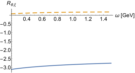
Figure 1: Ratio (IV.4) for the bulk hadron contribution $R_{\zeta}$ blue-solid curve vs $\omega$, and for the hadron shear contribution $R_{\eta}$ orange-dashed curve vs $\omega$ in the VDM approximation, for $\beta=1/m_{\pi}$, and equal relaxation times $t_{\zeta}=t_{\eta}=\beta$ for fixed $\theta=\sigma=1$.

For comparison, the (un-summed) equilibrium VDM rate (IV.3) in the same approximation reads

$$\frac{d^{3}\tilde{\Gamma}^{<}_{0}}{d^{3}k}\approx\frac{3\alpha}{8\pi^{4}}\frac{f_{A}^{2}m_{A}^{2}}{f_{\pi}^{2}\omega^{3}}\,\Gamma\,\int_{\frac{m_{\pi}\omega}{m_{A}^{2}}}^{\infty}dx\frac{x^{2}f_{1}(x)}{e^{\frac{\beta m_{A}^{2}x}{\omega}}-1}$$ (39)

where the lower bound stems from

$$(p+k)^{2}=2E\omega(1-\cos\theta_{p})=m_{A}^{2}$$ (40)

The ratio of the (un-summed) viscous rate (35) to the equilibrium rate (39) takes the simple form

$$\frac{d\Gamma^{<}_{1}}{d\Gamma^{<}_{0}}\approx-\frac{m_{A}^{2}}{2\omega}\left(\int_{\frac{m_{\pi}\omega}{m_{A}^{2}}}^{\infty}dx\frac{x^{2}f_{1}(x)}{e^{\frac{\beta m_{A}^{2}x}{\omega}}-1}\right)^{-1}$$

$$\times\biggl{(}2t_{\zeta}\theta\int_{\frac{m_{\pi}\omega}{m_{A}^{2}}}^{\infty}dx\frac{x^{3}e^{\frac{\beta m_{A}^{2}x}{\omega}}}{(e^{\frac{\beta m_{A}^{2}x}{\omega}}-1)^{2}}f_{1}(x)\biggr{.}$$

$$\biggl{.}\,\,\,\,\,\,+t_{\eta}\sigma\int_{\frac{m_{\pi}\omega}{m_{A}^{2}}}^{\infty}dx\frac{x^{3}e^{\frac{\beta m_{A}^{2}x}{\omega}}}{(e^{\frac{\beta m_{A}^{2}x}{\omega}}-1)^{2}}(3f_{2}(x)-f_{1}(x))\biggr{)}$$

In Fig. 1 we show the bulk contribution $R_{\zeta}$ in (IV.4) as the solid-blue curve, and the shear contribution $R_{\eta}$ in (IV.4) as the orange-dashed over a range of frequencies $\omega$ in GeV for a temperature $1/\beta=m_{\pi}$. We have set the shear and bulk factors to $\theta=\sigma=1$, and fixed the relaxation times to $t_{\eta}=t_{\zeta}=\beta$. The smallness of the shear contribution stems from the near cancellation of the $3f_{2}-f_{1}$ in the integrand of (IV.4). The bulk contribution dwarfs the shear contribution in the VDM approximation for about all frequencies. The bulk contribution is also opposite in sign to the shear contribution in leading order. At currently available collider energies, a typical AA collision triggers a hadronic fluid with a size $L\approx 10$ fm. For temperatures $T\approx 200$ MeV that results in fluid gradients of the size $\theta\approx\sigma\approx 1/TL\approx 1/10$. When combined with the result shown in Fig. 1, this estimate shows that the bulk viscosity correction to the hadronic rate is about 30% across all frequencies, while the shear viscosity correction is negligible. Overall, the bulk hydrodynamical correction appears sizable even in the late stage of the hadronic evolution with smal gradients in the form of a small $\theta=\partial_{i}\beta_{i}/3$. These observations deserve to be further checked in current hydrodynamical assessments of the electromagnetic emissivities and without the VDM approximation through the use of the full axial spectral weight.

IV.5 Viscous dilepton rate

The previous results, extend to the dilepton rates as well if we recall that for dilepton emissivities (1) need to be changed to

$$\frac{d\mathbb{R}_{0}}{d^{4}q}=-\frac{\alpha^{2}{\mathbb{B}}\,g^{\mu\nu}}{6\pi^{3}q^{2}}\left<\mathbb{G}_{\mu\nu}^{<}(q)\right>_{0}$$ (42)

with the leptonic factor

$$\mathbb{B}=\left(1+\frac{2m_{l}^{2}}{q^{2}}\right)\left(1-\frac{4m_{l}^{2}}{q^{2}}\right)^{\frac{1}{2}}$$ (43)

with the treshold $q^{2}>4m_{l}^{2}$ and typically $l=e,\mu$. The equilibrium contributions to (42) in the hadronic phase have been discussed in details using spectral functions in DILEPTON and hadronic processes in HADRON . From the spectral functions analysis the result is DILEPTON

$$\frac{d\mathbb{R}_{0}}{d^{4}q} =-\frac{\alpha^{2}}{6\pi^{3}}\frac{\mathbb{B}}{q^{2}}\,\frac{2}{e^{\beta\omega}+1}\,$$ (44)

$$\times\biggl{(}-3q^{2}{\rm Im}\Pi_{V}(q^{2})+\int\frac{d^{3}p}{(2\pi)^{3}}\frac{1}{2E}\frac{1}{e^{\beta E}-1}$$

$$\times\biggl{(}\frac{12}{f_{\pi}^{2}}q^{2}\text{Im}{\bf\Pi}_{V}(q^{2})$$

$$-\frac{6}{f_{\pi}^{2}}(p-q)^{2}\text{Im}{\bf\Pi}_{A}\left((p-q)^{2}+q\rightarrow-q\right)$$

$$+\frac{8}{f_{\pi}^{2}}\left((p\cdot q)^{2}-m_{\pi}^{2}q^{2}\right)\text{Im}{\bf\Pi}_{V}(q^{2})\times\text{Re}\Delta_{R}(p-q)$$

$$+q\rightarrow-q\biggr{)}\biggr{)}$$

The non-equilibrium viscous correction in the hadronic phase, follows a similar reasoning as that given for the photons. A rerun of the preceding reasoning shows that $G^{<}_{ij,0\pi}$ also vanishes in this case. However, $G^{<}_{1\pi}$ does not and the result is

$$(d\pi)_{ij}G^{<}_{1\pi}(q,k)=\frac{d^{3}k}{(2\pi)^{3}}\frac{t_{H}}{2E}\left(\frac{k_{i}k_{j}}{E_{k}}\right)n_{B}(1+n_{B})$$

$$\times\biggl{(}\frac{12}{f_{\pi}^{2}}q^{2}\text{Im}{\bf\Pi}_{V}(q^{2})$$

$$-\frac{6}{f_{\pi}^{2}}(k-q)^{2}\text{Im}{\bf\Pi}_{A}\left((k-q)^{2}\right)$$

$$+\frac{8}{f_{\pi}^{2}}\left((k\cdot q)^{2}-m_{\pi}^{2}q^{2}\right)\text{Im}{\bf\Pi}_{V}(q^{2})\times\text{Re}\Delta_{R}(k-q)\biggr{)}$$

Here $\Pi_{V}$ is the VV correlation of the vector current in the vacuum, and $\Delta_{R}$ is the retarded pion propagator STEELE . The spectral form of $\Pi_{V}$ follows from $e^{+}e^{-}$ annihilation. The last bracket in (IV.5) is only the crossed $\gamma^{*}\pi\rightarrow\gamma^{*}\pi$ scattering amplitude ${\cal T}_{\gamma^{*}\pi}$, which is seen to reduce to (IV.2) at the photon point or $q^{2}=0$. In terms of (IV.5) the re-summed viscous corrections to the dilepton emissivities in a hadronic fluid take the following final form

$$\frac{d\mathbb{R}_{1}}{d^{4}q} =-\frac{4\alpha^{2}}{3\pi^{2}}\frac{\mathbb{B}}{q^{2}}\,\frac{1}{e^{\beta\omega}+1}\,\int\frac{p^{4}dp\,d{\rm cos}\theta_{p}}{(2\pi)^{3}}\frac{1}{2E}\frac{e^{\beta E}}{(e^{\beta E}-1)^{2}}$$ (46)

$$\times\left(\left(t_{\zeta}\theta-\frac{1}{2}t_{\eta}\sigma\right)+\frac{3}{2}t_{\eta}\sigma\cos^{2}\theta_{p}\right)$$

$$\times\biggl{(}\frac{12}{f_{\pi}^{2}}q^{2}\text{Im}{\bf\Pi}_{V}(q^{2})$$

$$-\frac{6}{f_{\pi}^{2}}(p-q)^{2}\text{Im}{\bf\Pi}_{A}\left((p-q)^{2}+q\rightarrow-q\right)$$

$$+\frac{8}{f_{\pi}^{2}}\left((p\cdot q)^{2}-m_{\pi}^{2}q^{2}\right)\text{Im}{\bf\Pi}_{V}(q^{2})\times\text{Re}\Delta_{R}(p-q)$$

$$+q\rightarrow-q\biggr{)}$$

The total viscous hadronic rate for dilepton emission is (44) plus (46)

$$\frac{d\mathbb{R}}{d^{4}q}=\frac{d\mathbb{R}_{0}}{d^{4}q}+\frac{d\mathbb{R}_{1}}{d^{4}q}$$ (47)

V Partonic phase

At high temperature the fluid is that of strongly coupled partonic-like constituents (sQGP). We will treat it in leading order as made of partonic constituents in the presence of soft gluonic fields. The soft corrections will be estimated as operator insertions in leading dimensions as in OPE . A similar proposal using soft insertions for the electromagnetic emissivities was also suggested in ROB . With this in mind, and for the generic process $[p_{i}]\rightarrow[q_{f}]+\gamma$, the unordered Wightman function reads LARRY ,

$$-G^{\mu<}_{\mu}(q)=$$

$$\int\prod_{i}\frac{d^{3}p^{\rm in}_{i}}{(2\pi)^{3}2E_{i}^{\rm in}}n(E_{i}^{\rm in})\prod_{j}\frac{d^{3}q^{\rm out}_{j}}{(2\pi)^{3}2E_{j}^{\rm out}}(1\pm n(E_{j}^{\rm out}))$$

$$\times(2\pi)^{4}\delta\left(\sum_{i}{p_{i}}-\sum_{j}{q_{j}}-{q}\right)\,|{\bf M}_{i\rightarrow f+\gamma}|^{2}$$ (48)

The effects of the viscous corrections amount to additional contributions to the initial and final distribution functions. We now detail them for both dilepton and photon emissions.

V.1 Dileptons

We now seek to organize the photon emissivities in the non-perturbative partonic phase as follows

$$\frac{d^{3}\mathbb{R}}{d^{4}q}=\frac{d^{3}\mathbb{R}^{Tp}_{0}}{d^{4}q}+\frac{d^{3}\mathbb{R}^{Vp}_{1}}{d^{4}q}+\frac{d^{3}\mathbb{R}^{Tn}_{0}}{d^{4}q}+\frac{d^{3}\mathbb{R}^{Vn}_{1}}{d^{4}q}$$ (49)

with the first contribution $\mathbb{R}^{Tp}_{0}$ as the thermal perturbative rate, the second contribution $\mathbb{R}^{Vp}_{1}$ as the viscous perturbative correction, the third contribution $\mathbb{R}^{Tn}_{0}$ as the thermal and non-perturbative correction of leading mass dimension in the external fields, and finally the fourth contribution $\mathbb{R}^{Vp}_{1}$ as the viscous non-perturbative contribution in leading mass dimension in the external fields. We now proceed to evaluate each of these contributions sequentially as (54), (V.1.2), (66) and (V.1.4) to be detailed below.

V.1.1 Thermal perturbative contribution

In leading order, the perturbative dilepton emissivity corresponds to an in-state with a single $q\bar{q}$ as illustrated in Fig. 3, and its contribution to (V) is (omitting all charge factors)

$$-G^{\mu<}_{\mu}(q)=\frac{q^{2}}{\pi|q|}\int_{\frac{q_{0}-|q|}{2}}^{\frac{q_{0}+|q|}{2}}dkf_{\mu}(k)f_{-\mu}(q_{0}-k)$$

$$=n_{B}(q_{0})\,\frac{q^{2}}{\pi|q|}\int_{q^{-}}^{q^{+}}(1-f_{\mu}(k)-f_{-\mu}(q_{0}-k))$$

$$=n_{B}(q_{0})\,\frac{q^{2}}{\pi}n_{B}(q_{0})\left(-1+\frac{1}{\beta|q|}\rm ln\left(\frac{n_{\mu}^{-}n_{-\mu}^{-}}{n_{\mu}^{+}n_{-\mu}^{+}}\right)\right)$$ (50)

we have defined the Fermi distributions at finite chemical potential $\mu$ as

$$f_{\pm\mu}(q)=\frac{1}{e^{\beta({q_{0}\mp\mu})}+1}$$ (51)

and their associated shifted distributions

$$n_{\pm\mu}^{\pm}=\frac{1}{e^{\beta(q_{0}\pm|q|)/2\mp\beta\mu}+1}$$ (52)

The emergence of the Bose distribution $n_{B}=1/(e^{\beta q_{0}}-1)$ in (V.1.1) reflects on the KMS condition

$$G^{\mu<}_{\mu}(q)=2n_{B}(q_{0})\,{\rm Im}\,iG^{\mu R}_{\mu}(q)$$ (53)

at finite temperature and chemical potential $\mu$ in leading order. The finite chemical potential will be traded below for a complex chemical potential for a fixed color species and identified with the insertion of a soft $A_{4}$ contribution in the strongly coupled QGP OPE ; ROB . For $\mu=0$, (V.1.1) when inserted in the general formula for dilepton emission (42) and upon restoring the color-flavor factor for partons $N_{c}\hat{e}_{f}^{2}/2$, yield the leading partonic dilepton rate

$$\frac{d\mathbb{R}^{T}_{0}}{d^{4}q} =\frac{-\alpha^{2}\mathbb{B}}{3\pi^{3}}\frac{1}{e^{\beta q_{0}}-1}$$ (54)

$$\times\left(\frac{1}{4\pi}\,d_{F}\sum_{f}\hat{e}_{f}^{2}\right)\left(1+\frac{2}{\beta|q|}\,{\rm ln}\left(\frac{n^{+}}{n^{-}}\right)\right)$$

with $d_{F}=N_{c}$ the color dimension of the quark representation, and $n^{\pm}\equiv n^{\pm}_{\pm 0}$. Here $e\hat{e}_{f}$ is the electromagnetic charge of a quark of flavor $f$. In this order, the emission is isotropic.

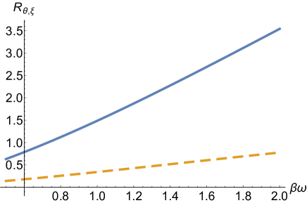
Figure 2: Ratio $d{\mathbb{R}_{1}^{Vp}}/d{\mathbb{R}_{0}^{Tp}}$ for the thermal perturbative dilepton bulk contribution $R_{\zeta}$ blue-solid curve vs $\beta\omega$, and for the thermal perturbative shear dilepton contribution $R_{\eta}$ orange-dashed curve vs $\beta\omega$ and $q=(2\omega,\omega)$. We have set the relaxation times $t_{\zeta}=t_{\eta}=\beta$ and fixed $\theta=\sigma=1$.

V.1.2 Viscous perturbative contribution

The viscous corrections to the perturbative quark and gluon processes, follow exactly along the general arguments we presented earlier in sections II and III. Specifically, for the Fermionic Wightman functions

$$G_{\alpha\beta}^{>}(x)=+\left<\psi_{\alpha}(x)\bar{\psi}_{\beta}(0)\right>$$

$$G_{\alpha\beta}^{<}(x)=-\left<\bar{\psi}_{\beta}(0)\psi_{\alpha}(x)\right>$$ (55)

the $T_{ij}$ insertions amounts to additional contributions, and in leading order we have

$$G^{<}(k)=-\frac{\pi\not{k}}{E}n(k_{0})(\delta^{-}-\delta^{+})$$

$$-t_{H}\partial_{i}\beta_{j}\frac{k^{i}k^{j}}{E}\frac{\pi\not{k}}{E}n(k_{0})(1-n(k_{0}))(\delta^{-}+\delta^{+})$$

$$G^{>}(k)=+\frac{\pi\not{k}}{E}(1-n)(\delta^{-}-\delta^{+})$$

$$-t_{H}\partial_{i}\beta_{j}\frac{k^{i}k^{j}}{E}\frac{\pi\not{k}}{E}n(1-n)(\delta^{-}+\delta^{+})$$ (56)

with $\delta^{\pm}\equiv\delta(k_{0}\mp k)$. In the real-time or double-line formalism, the total emission rate follows from the 12 Wightman function, where the effects of the $T_{ij}$ insertions amount to modifying the in-state population by

$$n\rightarrow n+t_{H}\frac{k_{i}k_{j}}{E}\partial_{i}\beta_{j}\,n(1\pm n)$$ (57)

and the out-state population by

$$n\rightarrow 1-n-t_{H}\frac{k_{i}k_{j}}{E}\partial_{i}\beta_{j}\,n(1\pm n)$$ (58)

With this in mind, the viscouss corrections to the leading order dilepton emission at finite chemical potential (V.1.1) is

$$+t_{H}\partial_{i}\beta_{j}\frac{q^{2}}{\pi|q|}\int_{\frac{q_{0}-|q|}{2}}^{\frac{q_{0}+|q|}{2}}dkf_{\mu}(1-f_{\mu})f_{-\mu}(q_{0}-k)\frac{k_{i}k_{j}}{k}$$

$$+t_{H}\partial_{i}\beta_{j}\frac{q^{2}}{\pi|q|}\int_{\frac{q_{0}-|q|}{2}}^{\frac{q_{0}+|q|}{2}}dkf_{-\mu}(1-f_{-\mu})f_{\mu}(q_{0}-k)\frac{k_{i}k_{j}}{k}$$

which can be re-organized as follows

$$t_{H}\partial_{i}\beta_{j}\frac{q^{2}}{\pi|q|}$$

$$\times\biggl{(}\frac{\delta_{ij}-\hat{q}_{i}\hat{q}_{j}}{2}\int_{\frac{q_{0}-|q|}{2}}^{\frac{q_{0}+|q|}{2}}dkkf_{\mu}(1-f_{\mu})f_{-\mu}(q_{0}-k)\biggr{.}$$

$$\biggl{.}+\frac{3\hat{q}_{i}\hat{q}_{j}-\delta_{ij}}{2}\int_{\frac{q_{0}-|q|}{2}}^{\frac{q_{0}+|q|}{2}}dkkf_{\mu}(1-f_{\mu})f_{-\mu}(q_{0}-k)\biggr{.}$$

$$\biggl{.}\times\left(\frac{q_{0}}{|q|}-2\frac{q_{+}q_{-}}{|q|k}\right)^{2}+\mu\rightarrow-\mu\biggr{)}$$ (60)

The $\mu=0$ contribution in (V.1.2) yields the viscous perturbative contribution to the dilepton rate (54). More specifically, we have

$$\frac{d\mathbb{R}^{Vp}_{1}}{d^{4}q} =\frac{\alpha^{2}\mathbb{B}}{3\pi^{3}}\frac{1}{e^{\beta q_{0}}-1}$$

$$\times\left(\frac{1}{4\pi}\,d_{F}\sum_{f}\hat{e}_{f}^{2}\right)\,\frac{2}{|q|}$$

$$\times\biggl{(}\frac{2t_{\zeta}\theta-t_{\eta}\sigma}{2}\int_{\frac{q_{0}-|q|}{2}}^{\frac{q_{0}+|q|}{2}}dkk(1-f-\tilde{f})(1-f)\biggr{.}$$

$$\biggl{.}+\frac{3t_{\eta}\sigma}{2}\int_{\frac{q_{0}-|q|}{2}}^{\frac{q_{0}+|q|}{2}}dkk(1-f-\tilde{f})(1-f)\biggr{.}$$

$$\biggl{.}\times\left(\frac{q_{0}}{|q|}-2\frac{q_{+}q_{-}}{|q|k}\right)^{2}\biggr{)}$$

where we have defined the fermionic distributions $f\equiv f_{0}(k)$ and $\tilde{f}\equiv f_{0}(q_{0}-k)$ for $\mu=0$.

In Fig. 2 we show the ratio $d{\mathbb{R}_{1}^{Vp}}/d{\mathbb{R}_{0}^{Tp}}$ of the thermal viscous contribution (V.1.2) to the free thermal contribution (54), for dilepton emission at $q=(2\omega,\omega)$ as a function of $\beta\omega$, after setting $t_{\zeta}=t_{\eta}=\beta$ and $\theta=\sigma=1$. The orange-dashed line is the shear ratio, while the blue-solid line is the bulk ratio. Again, the bulk contribution is larger than the shear contribution and both are positive and increasing with $\beta\omega$.

Figure 3: Thermal dilepton emission including the leading perturbative term (top) and the leading soft and non-perturbative corrections (bottom). The blob refers to gluon insertions of leading dimensions $(gA_{4})^{2},(gE)^{2},(gB)^{2}$.

V.1.3 Thermal non-perturbative contribution

The partonic phase near the transition temperature still carries soft gluons OPE ; ROB . Their effects is to modify both the thermal and viscous rates. A way to assess these non-perturbative effects is to organize these modifications as power corrections through gluonic operators insertions of increasing dimension $\Delta=2,4$ in the $JJ$ correlation function. In Fig. 3 we illustrate the leading soft gluonic insertions on the dilepton emissivities. Typically, these contributions are of the form $(gA_{4})^{2},(gE)^{2},(gB)^{2},...$ and of order $(g^{2}T)^{\Delta}$.

Since a constant $gA_{4}$ acts as an imaginary colored chemical potential on the quark line, the leading operator insertion $(gA_{4})^{2}$ is readily obtained from the quadratic $\mu$-contribution steming from the fermionic propagator at finite chemical potential, with the identification

$$\mu^{2}\rightarrow-\left<(gA_{4})^{2}\right>$$ (62)

A proof of this is given in the Appendix A using the background field method. With this in mind, the quadratic contribution steming from (V.1.1) is

$$\rm ln\left(\frac{n_{\mu}^{-}n_{-\mu}^{-}}{n_{\mu}^{+}n_{-\mu}^{+}}\right)=+2\,\rm ln\left(\frac{n^{-}}{n^{+}}\right)$$

$$+(\beta\mu)^{2}(n^{+}(1-n^{+})-n^{-}(1-n^{-}))+{\cal O}(\mu^{4})$$ (63)

which corrects the perturbative dilepton rate (54) by the non-perturbative contribution

$$-\frac{\alpha^{2}\mathbb{B}}{3\pi^{3}}\frac{1}{e^{\beta q_{0}}-1}\left(\frac{1}{4\pi}\,d_{F}\sum_{f}\hat{e}_{f}^{2}\right)\left<(gA_{4})^{2}\right>$$

$$\times\left(\frac{\beta}{|q|}\right)\left(n^{+}(1-n^{+})-n^{-}(1-n^{-})\right)$$ (64)

The effects of $(gE)^{2},(gB)^{2}$ can be calculated by general arguments using the background field method OPE , as briefly recalled in the Appendix. The net result can be understood using the following simple substitution

$$\left<(gA_{4})^{2}\right>\rightarrow\left<(gA_{4})^{2}\right>-\frac{1}{6q^{2}}\left<(gE)^{2}\right>+\frac{1}{3q^{2}}\left<(gB)^{2}\right>$$ (65)

a proof of which is given in Appendix A. The substitution can be understood as $(gqA_{4})\sim gE\sim gB$. The factor of $\frac{1}{3}$ is from averaging over the vector orientations. The extra $-\frac{1}{2}$ in front of the electric contribution is due to the use of a fixed thermal frame and the fact that $(gE)^{2}\sim-(gB)^{2}$ in Euclidean space. Hence the final non-perturbative corrections to the dilepton rate (54) in leading operator insertions

$$\frac{d{\mathbb{R}}^{Tn}_{0}}{d^{4}q} =\frac{\alpha^{2}\mathbb{B}}{3\pi^{3}}\frac{1}{e^{\beta q_{0}}-1}\left(\frac{1}{4\pi}\,d_{F}\sum_{f}\hat{e}_{f}^{2}\right)$$ (66)

$$\times\left(-\left<(gA_{4})^{2}\right>+\frac{1}{6q^{2}}\left<(gE)^{2}\right>-\frac{1}{3q^{2}}\left<(gB)^{2}\right>\right)$$

$$\times\left(\frac{\beta}{|q|}\right)\left(n_{+}(1-n_{+})-n_{-}(1-n_{-})\right)\biggr{)}$$

in agreement with the result in OPE . The typical values of the soft condensate insertions in (66) are discussed in OPE ; Lee14 .

V.1.4 Viscous non-perturbative contribution

The viscous and non-perturbative corrections to (V.1.2) can be obtained using the same reasoning developed above for the non-perturbative thermal corrections. For that, we expand the general result (V.1.2) to quadratic order in $\mu$, by expanding the fermionic occupation number

$$f_{\mu}=f+\beta\mu f(1-f)+\frac{1}{2}{(\beta\mu)^{2}}\,f(1-f)(1-2f)+{\cal O}(\mu^{3})$$

Now we use the identity

$$\int f_{\mu}(1-f_{\mu})f_{-\mu}(q_{0}-k)\,[...]=$$

$$n_{B}(q_{0})\int(1-f_{\mu}-f_{-\mu}(q_{0}-k))(1-f_{\mu})\,[...]$$ (68)

and expand the integrand in $\mu$. The quadratic contribution reads

$$\biggl{(}(1-f_{\mu}-\tilde{f}_{-\mu})(1-f_{\mu})+(\mu\rightarrow-\mu)\biggr{)}_{\mu^{2}}=$$

$$+2f(1-f)^{2}(3f-1)+f(1-f)(1-2f)(\tilde{f}-1)$$

$$+\tilde{f}(1-\tilde{f})(1-2\tilde{f})(f-1)-2f(1-f)\tilde{f}(1-\tilde{f})$$

With the help of the identity

$$2f(1-f)^{2}(3f-1)=$$

$$(1+n_{B}(q_{0}))(1-\tilde{f}-f)(f(1-2f)+\tilde{f}(1-2\tilde{f}))$$

$$-2n_{B}(q_{0})(1+n_{B}(q_{0})(1-f-\tilde{f})^{2}$$ (70)

we have finally for the $\mu^{2}$ correction to the viscous corrections to (V.1.2) as

$$(\beta\mu)^{2}t_{H}\partial_{i}\beta_{j}\frac{q^{2}}{\pi|q|}\times$$

$$\biggl{(}\frac{\delta_{ij}-\hat{q}_{i}\hat{q}_{j}}{2}(n_{B}F_{1}+n_{B}(1+n_{B})F_{2}+n_{B}^{2}(1+n_{B})F_{3})\biggr{.}$$

$$\biggl{.}+\frac{3\hat{q}_{i}\hat{q}_{j}-\delta_{ij}}{2}(n_{B}\tilde{F}_{1}+n_{B}(1+n_{B})\tilde{F}_{2}+n_{B}^{2}(1+n_{B})\tilde{F}_{3})\biggr{)}$$

where we have defined

$$F_{1}= +2\int dkkf(1-f)^{2}(3f-1)$$

$$\tilde{F}_{1}= +2\int dkkf(1-f)^{2}(3f-1)\left(\frac{q_{0}}{|q|}-\frac{2q_{+}q_{-}}{|q|k}\right)^{2}$$

$$F_{2}= -\int dkk(1-\tilde{f}-f)(f(1-2f)+\tilde{f}(1-2\tilde{f}))$$

$$\tilde{F}_{2}= -\int dkk(1-\tilde{f}-f)(f(1-2f)+\tilde{f}(1-2\tilde{f}))$$

$$\times\left(\frac{q_{0}}{|q|}-\frac{2q_{+}q_{-}}{|q|k}\right)^{2}$$

$$F_{3}= -2\int dkk(1-\tilde{f}-f)^{2}\$$

$$\tilde{F}_{3}= -2\int dkk(1-\tilde{f}-f)^{2}\left(\frac{q_{0}}{|q|}-\frac{2q_{+}q_{-}}{|q|k}\right)^{2}$$ (72)

Using the operator substitutions (62-65) for $\mu^{2}$ in (V.1.4) lead to the non-perturbative corrections to the viscous dilepton emission rate (V.1.2) in the form $(n_{B}\equiv n_{B}(q_{0}))$

$$\frac{d\mathbb{R}^{Vn}_{1}}{d^{4}q}=\frac{\alpha^{2}\mathbb{B}}{3\pi^{3}q^{2}}\frac{\beta^{2}}{e^{\beta q_{0}}-1}$$

$$\times\left(\frac{1}{4\pi}\,d_{F}\sum_{f}\hat{e}_{f}^{2}\right)\,\frac{q^{2}}{\pi|q|}$$

$$\times\left(-\left<(gA_{4})^{2}\right>+\frac{1}{6q^{2}}\left<(gE)^{2}\right>-\frac{1}{3q^{2}}\left<(gB)^{2}\right>\right)$$

$$\biggl{(}\frac{2t_{\zeta}\theta-t_{\eta}\sigma}{2}(n_{B}F_{1}+n_{B}(1+n_{B})F_{2}+n_{B}^{2}(1+n_{B})F_{3})\biggr{.}$$

$$\biggl{.}+\frac{3t_{\eta}\sigma}{2}(n_{B}\tilde{F}_{1}+n_{B}(1+n_{B})\tilde{F}_{2}+n_{B}^{2}(1+n_{B})\tilde{F}_{3})\biggr{)}$$

Figure 4: Thermal photon emission including the leading perturbative term and the leading soft and non-perturbative corrections. The blob refers to gluon insertions of leading dimensions $(gA_{4})^{2},(gE)^{2},(gB)^{2}$. Soft vertex insertions as in Fig.3 are also included but not shown. The last two contributions are not allowed without the soft insertions.

V.2 Photons

Following the dilepton analysis, we now seek to organize the photon emissivities in the non-perturbative partonic phase as follows

$$\frac{d^{3}\Gamma}{d^{3}k}=\frac{d^{3}\Gamma^{Tp}_{0}}{d^{3}k}+\frac{d^{3}\Gamma^{Vp}_{1}}{d^{3}k}+\frac{d^{3}\Gamma^{Tn}_{0}}{d^{3}k}+\frac{d^{3}\Gamma^{Vn}_{1}}{d^{3}k}$$ (74)

with the first contribution $\Gamma^{Tp}_{0}$ as the thermal perturbative rate, the second contribution $\Gamma^{Vp}_{1}$ as the viscous perturbative correction, the third contribution $\Gamma^{Tn}_{0}$ as the thermal and non-perturbative correction of leading mass dimension in the external fields, and finally the fourth contribution $\Gamma^{Vp}_{1}$ as the viscous non-perturbative contribution in leading mass dimension in the external fields. We now proceed to evaluate each of these contributions sequentially as (V.2.2), (96), (102) and (V.2.5) to be detailed below.

V.2.1 General

The photon analysis is more involved since the in-state with $q\bar{q}$ is kinematically not allowed. The partonic photon emission proceeds through: 1/ the Compton channel, with $qg\rightarrow\gamma q$ or $\bar{q}g\rightarrow\gamma\bar{q}$; 2/ the pair annihilation channel with $\bar{q}q\rightarrow g\gamma$, as illustrated in Fig. 4. Specifically, we have

$$G^{<}_{\rm compton}=\frac{{\bf N}}{8(2\pi)^{4}E}\int dsdt|M_{c}(s,t)|^{2}$$

$$\times\int dE_{1}dE_{2}f_{\mu}(E_{1})f_{g}(E_{2})(1-f_{\mu}(E_{1}+E_{2}-E))$$

$$\times\frac{\theta(E_{1}+E_{2}-E)}{\sqrt{aE_{1}^{2}+bE_{1}+c}}+\mu\rightarrow-\mu$$ (75)

with $E=\omega=k$ throughout, and

$$G^{<}_{\rm pair}=\frac{{\bf N}}{8(2\pi)^{4}E}\int dsdt|M_{p}(s,t)|^{2}$$

$$\times\int dE_{1}dE_{2}f_{\mu}(E_{1})f_{-\mu}(E_{2})(1+f_{g}(E_{1}+E_{2}-E))$$

$$\times\frac{\theta(E_{1}+E_{2}-E)}{\sqrt{aE_{1}^{2}+bE_{1}+c}}$$ (76)

The leading perturbative contributions to the squared matrix elements are

$$\frac{|M_{c}(s,t,u)|^{2}}{16\pi^{2}}=-8\alpha\alpha_{s}\frac{u^{2}+s^{2}}{us}$$

$$\frac{|M_{p}(s,t,u)|^{2}}{16\pi^{2}}=+8\alpha\alpha_{s}\frac{u^{2}+t^{2}}{ut}$$ (77)

and the color-flavor factor is

$${\bf N}=\frac{N_{c}^{2}-1}{2N_{c}}N_{c}\sum_{f}\hat{e}_{f}^{2}\equiv C_{F}d_{F}\sum_{f}\hat{e}_{f}^{2}$$ (78)

The Mandelstam variables and the kinematical parameters $a,b,c$ are collectively defined as

$$s=(p_{1}+p_{2})^{2}$$

$$t=(p-p_{1})^{2}$$

$$a=-(s+t)^{2}$$

$$b=2(s+t)(Es-E_{2}t)$$

$$c=st(s+t)-(Es+E_{2}t)^{2}$$ (79)

with $s+t+u=0$. The range of the integrations are $s\geq 0$ and $-s\leq t\leq 0$. However, the $s$-integration is infrared sensitive, so the integration range will be modified to $s\geq m_{T}^{2}$ with the squared thermal quark mass $m_{T}^{2}=\pi\alpha_{s}C_{F}/\beta^{2}$ as a regulator. These results are in agreement with those first reported in NAIVE .

V.2.2 Thermal perturbative contribution

In this section we will detail the approximations in the reduction of (V.2.1-V.2.1) in leading order, as they will be used for the viscous contributions as well. Following NAIVE we can unwind the integrations through the Boltzmann approximation

$$f_{0}(E_{1})f_{g}(E_{2})\sim e^{-\beta(E_{1}+E_{2})}\sim e^{-\beta E}$$ (80)

in terms of which the integrand is typically of the form

$$\int dE_{1}dE_{2}f(E_{1}+E_{2}-E)\frac{\theta(E_{1}+E_{2}-E)}{\sqrt{aE_{1}^{2}+bE_{1}+c}}$$ (81)

After the change of variables $E_{1}=x^{\prime}+y,E_{2}=x^{\prime}-y$, this integral simplifies

$$2\int dx^{\prime}\int dy\frac{f(2x^{\prime}-E)}{\sqrt{s^{2}(y-y_{2})(y_{1}-y)}}$$ (82)

with the integration over y giving just $\frac{\pi}{s}$. From the constraint

$$2(E_{1}+E_{2}-E)E(1-\cos\theta_{34})=s$$ (83)

we find that $2x^{\prime}-E=2x\geq\frac{s}{8E}$, and (81) gives

$$\frac{2\pi}{s}\int_{\frac{s}{8E}}^{\infty}dx\,f(2x)$$ (84)

For either distributions $f=\frac{1}{e^{\beta x}\pm 1}$ we obtain

$$\frac{\pi}{\beta s}\rm ln(1\pm e^{-\frac{\beta s}{4E}})^{\pm 1}$$ (85)

The $t$-integrations can be carried explicitly with the results

$$\int\frac{dt}{s}{|M_{c}(s,t)|^{2}}$$

$$=128\pi^{2}\alpha\alpha_{s}\left({\rm ln}\left(\frac{s-m_{T}^{2}}{m_{T}^{2}}\right)+\frac{1}{2}\left(1-\frac{2m_{T}^{2}}{s}\right)\right)$$

$$\int\frac{dt}{s}{|M_{p}(s,t)|^{2}}$$

$$=256\pi^{2}\alpha\alpha_{s}\left({\rm ln}\left(\frac{s-m_{T}^{2}}{m_{T}^{2}}\right)-\left(1-\frac{2m_{T}^{2}}{s}\right)\right)$$ (86)

Again, the infrared cutoff satisfies $2m_{T}^{2}\leq s$ ,$-s+m_{T}^{2}\leq t\leq-m_{T}^{2}$. With the above in mind, the leading equilibrium photon emission from a perturbative QCD plasma associated to the Compton $qg\rightarrow q\gamma$ and pair creation $q\bar{q}\rightarrow\gamma g$ processes, is NAIVE

$$\frac{d\Gamma^{T}_{0}}{d^{3}k} =\frac{\alpha\alpha_{s}}{\pi}\frac{1}{E\beta^{2}}\frac{1}{e^{\beta E}-1}$$

$$\times\left(\frac{1}{4\pi}\,C_{F}d_{F}\sum_{f}\hat{e}_{f}^{2}\right)\,\left(\frac{1}{2}{\rm ln}\left(\frac{4E}{\beta m_{T}^{2}}\right)+{\rm}{\bf C}\right)$$

Here ${\bf C}$ is a constant. The emission rate to this order is isotropic. In (V.2.2) the overall substitution

$$e^{-\beta E}\rightarrow\frac{1}{e^{\beta E}-1}$$ (88)

was made to recover the causal pre-factor required by the KMS condition for the retarded process as in (53).

Finally, we remark that the perturbative photon rate (V.2.2) receives additional perturbative corrections to the same order in $\alpha\alpha_{s}$ through collinear Bremsstralung AMY . This effect and its resummation will not be discussed here. Instead, we will focus on the potentially soft gluonic corrections that are also important near the transition temperature as we now detail.

V.2.3 Viscous perturbative contributions

As we noted in the dilepron rates above, the viscous corrections in leading order correspond to the partinent insertions of $k_{i}k_{j}$ on the partonic lines as given in (57-58). These gradient insertions break the isotropic character of the integrations with the typical integral structures

$$q_{i}q_{j}\int{\rm cos}^{2}\theta+\frac{(\delta_{ij}-q_{i}q_{j})}{2}\int(1-{\rm cos}^{2}\theta)$$

$$=q_{i}q_{j}\int\frac{3\,{\rm cos}^{2}\theta-1}{2}+\delta_{ij}\int\frac{1-{\rm cos}^{2}\theta}{2}$$ (89)

where the scattering angles are defined as

$${\rm cos}\,\theta_{1}=\frac{t+2EE_{1}}{2EE_{1}}$$

$${\rm cos}\,\theta_{2}=\frac{u+2EE_{2}}{2EE_{2}}$$

$${\rm cos}\,\theta_{3}=\frac{2(E_{1}+E_{2}-E)E-s}{2E(E_{1}+E_{2}-E)}$$ (90)

The angles $\theta_{1,2,3}$ refer to the angles between particle $1,2,3$ and $\gamma$ flying along the z-direction, in the process labeled as $1+2\rightarrow 3+\gamma$. To proceed, we now make two kinematical approximations to simplify the integration analyses to follow. The first is to follow (107) and approximate the population factors by

$$f_{\pm\mu}(E_{1})(1-f_{\pm\mu}(E_{1}))f_{g}(E_{2})\approx e^{-\beta(E_{1}+E_{2}\mp\mu)}$$

$$f_{\pm\mu}(E_{1})(f_{g})(1+f_{g})\approx e^{-\beta(E_{1}+E_{2}\mp\mu)}$$

and the second is to replace $E_{1,2}$ in ${\rm cos}(\theta_{1,2})$ by $E_{1,2}\approx(E_{1}+E_{2})/2$. These approximations will allow us to extract explicit estimates for the viscous perturbative and non-perturbative effects. They will be tested against realistic hydrodynamical evolution of the rates in the future. With this in mind the viscous corrections to the Compton (V.2.1) and pair (V.2.1) are respectively given by

$$-G^{<}_{c}=t_{H}\partial_{i}\beta_{j}\left(\frac{\delta_{ij}-\hat{q}_{i}\hat{q}_{j}}{2}G_{c}^{P}+\frac{3\hat{q}_{i}\hat{q}_{j}-\delta_{ij}}{2}G_{c}^{T}\right)$$

$$-G^{<}_{p}=t_{H}\partial_{i}\beta_{j}\left(\frac{\delta_{ij}-\hat{q}_{i}\hat{q}_{j}}{2}G_{p}^{P}+\frac{3\hat{q}_{i}\hat{q}_{j}-\delta_{ij}}{2}G_{p}^{T}\right)$$

with the Compton kernels

$$G_{c}^{P}\approx \frac{{\bf N}}{8(2\pi)^{3}E}\frac{1}{e^{\beta(E-\mu)}-1}\int\frac{dsdt}{s}\,{|M_{c}(s,t)|^{2}}$$

$$\times\int_{\frac{s}{8E}}^{\infty}dx\left(\frac{2x+E}{e^{\beta(2x-\mu)}+1}-\frac{2xe^{\beta(2x-\mu)}}{(e^{\beta(2x-\mu)}+1)^{2}}\right)$$

$$+\mu\rightarrow-\mu$$

$$G_{c}^{T}\approx \frac{{\bf N}}{8(2\pi)^{3}E}\frac{1}{e^{\beta(E-\mu)}-1}\int\frac{dsdt}{s}\,{|M_{c}(s,t)|^{2}}$$ (93)

$$\times\int_{\frac{s}{8E}}^{\infty}dx\biggl{(}\frac{2x+E-\frac{s}{E}+\frac{t^{2}+(s+t)^{2}}{8xE^{2}}}{e^{\frac{2x-\mu}{T}}+1}$$

$$\qquad\qquad\,\,\,-\frac{2xe^{\beta(2x-\mu)}(1-\frac{s}{4Ex})^{2}}{(e^{\beta(2x-\mu)}+1)^{2}}\biggr{)}$$

$$+\mu\rightarrow-\mu$$

and the pair production kernels

$$G_{p}^{P}\approx \frac{{\bf N}}{8(2\pi)^{3}E}\frac{1}{e^{\beta E}-1}\int\frac{dsdt}{s}\,{|M_{p}(s,t)|^{2}}$$

$$\times\int_{\frac{s}{8E}}^{\infty}dx\left(\frac{2x+E}{e^{\beta 2x}-1}+\frac{2xe^{\beta 2x}}{(e^{\beta 2x}-1)^{2}}\right)$$

$$G_{p}^{T}\approx \frac{{\bf N}}{8(2\pi)^{3}E}\frac{1}{e^{\beta E}-1}\int\frac{dsdt}{s}\,{|M_{p}(s,t)|^{2}}$$ (94)

$$\times\int_{\frac{s}{8E}}^{\infty}dx\biggl{(}\frac{2x+E-\frac{s}{E}+\frac{t^{2}+(s+t)^{2}}{8xE^{2}}}{e^{\beta 2x}-1}$$

$$\qquad\qquad\,\,\,+\frac{2xe^{\beta 2x}(1-\frac{s}{4Ex})^{2}}{(e^{\beta 2x}-1)^{2}}\biggr{)}$$

which are independent of the chemical potential $\mu$. In both kernels in (V.2.3-V.2.3) the substitution (88) was performed to recover the causal pre-factor required by the KMS condition. In terms of the hydrodynamical times, (V.2.3) reads

$$-G^{<}_{c}=\left(\frac{2t_{\zeta}\theta-t_{\eta}\sigma}{2}G_{c}^{P}+\frac{3t_{\eta}\sigma}{2}G_{c}^{T}\right)$$

$$-G^{<}_{p}=\left(\frac{2t_{\zeta}\theta-t_{\eta}\sigma}{2}G_{p}^{P}+\frac{3t_{\eta}\sigma}{2}G_{p}^{T}\right)$$

and the perturbative viscous correction to the photon rate takes the final form

$$\frac{d^{3}\Gamma^{\rm Vp}_{1}}{d^{3}k}=\frac{-1}{(2\pi)^{3}2E}(G^{<}_{c}+G^{<}_{p})_{\mu=0}$$ (96)

after setting $\mu=0$ in (V.2.3). In Appendix B, we explicit the contributions in (96). The ratio of the leading shear and bulk thermal contributions in (96) to the leading thermal perturbative photon contribution (V.2.2) are found to be

$$R_{\eta}=\frac{d^{3}\Gamma^{Vp}_{\rm shear}}{d^{3}\Gamma^{T}_{0}}\approx \left(E+\frac{1}{\beta}\left(A_{1}-2A_{2}-\frac{1}{3}-\frac{7\zeta_{3}}{\pi^{2}}\right)\right)\,t_{\eta}\sigma$$

$$R_{\zeta}=\frac{d^{3}\Gamma^{Vp}_{\rm bulk}}{d^{3}\Gamma^{T}_{0}}\approx \left(E+\frac{1}{\beta}\left(\frac{2}{3}+\frac{14\zeta_{3}}{\pi^{2}}\right)\right)\,t_{\zeta}\theta$$ (97)

with $E=\omega=k_{0}$. Here $A_{1,2}$ are functions of $E$ defined in (IX), that asymptote zero at large $E$ exponentially, and $\zeta_{3}$ referes to Riemann zeta function. In Fig. 5 we show the ratios (V.2.3) vs $\beta\omega$ with $\omega=E$, for $t_{\zeta}=t_{\eta}=\beta$ and fixed $\theta=\sigma=1$. The thermal viscous corrections to the photon emissivities become linearly large at large $E=\omega$. Since (V.2.3) were derived for large $E=\omega$, the low $E=\omega$ part of the curve receives additional corrections. Note that the constants contributions were dropped from both the perturbative and viscous rates at large $E=\omega$.

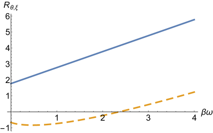
Figure 5: Ratios (V.2.3) for the photon thermal bulk contribution $R_{\zeta}$ blue-solid curve vs $\beta\omega$, and for the photon thermal shear contribution $R_{\eta}$ orange-dashed curve vs $\beta\omega$, and equal relaxation times $t_{\zeta}=t_{\eta}=\beta$ for fixed $\theta=\sigma=1$.

V.2.4 Thermal non-perturbative contributions

To obtain the thermal non-perturbative corrections to the photon rates we proceed as in the case of the dilepton rates above, by expanding (V.2.3) to order $\mu^{2}$ and then trading $\mu^{2}$ as in (62). With this in mind, we have

$$-G_{c}|_{\mu^{2}}=(\beta\mu)^{2}(G_{1}+G_{2})$$ (98)

with

$$G_{1}= \frac{{\bf N}}{16(2\pi)^{3}\beta E}n_{B}(1+n_{B})(1+2n_{B})$$

$$\times\int\frac{dsdt}{s}|M_{c}(s,t)|^{2}\rm ln(1+e^{-\frac{s}{4E}})$$

$$G_{2}= \frac{{\bf N}}{16(2\pi)^{3}\beta E}n_{B}\int\frac{dsdt}{s}|M_{c}(s,t)|^{2}\frac{e^{\frac{\beta s}{4}}}{(1+e^{\frac{\beta s}{4}})^{2}}$$

The associated non-perturbative photon rate is

$$-\frac{\beta^{2}}{(2\pi)^{3}2E}{\left<(gA_{4})^{2}\right>}(G_{1}+G_{2})_{\mu=0}$$ (100)

which corresponds to the leading soft gluon insertion to the Compton process. We now note that eventough the perturbative annihilation process $q\bar{q}\rightarrow\gamma$ is kinematically forbidden, its counterpart in the presence of external fields $(gE),(gB)$ is not. This contribution can be obtained from the $\gamma^{*}\rightarrow q\bar{q}$ process in (66) after suitably multiplying by $q^{2}$ and then taking $q^{2}\rightarrow 0$ to recover the photon point through the dilepton-photon identity

$$q_{0}\frac{d^{3}\Gamma}{d^{3}q}=\frac{3\pi}{2\alpha\mathbb{B}}\lim_{q^{2}\to 0}\left(q^{2}\frac{d^{4}{\mathbb{R}}}{d^{4}q}\right)$$ (101)

The outcome combined with (100) gives

$$\frac{d^{3}\Gamma^{Tn}_{0}}{d^{3}k}= \frac{\alpha}{2\pi^{2}E}\frac{1}{e^{\beta E}-1}\left(\frac{1}{4\pi}\,d_{F}\sum_{f}\hat{e}_{f}^{2}\right)$$ (102)

$$\times\left(\frac{1}{6}\left<(gE)^{2}\right>-\frac{1}{3}\left<(gB)^{2}\right>\right)$$

$$\times\left(\frac{\beta}{|q|}\right)\left(n_{+}(1-n_{+})-n_{-}(1-n_{-})\right)\biggr{)}$$

$$-\frac{\beta^{2}}{(2\pi)^{3}2E}{\left<(gA_{4})^{2}\right>}(G_{1}+G_{2})_{\mu=0}$$

The explicit forms of $G_{1,2}$ follow the same analysis detailed in Appendix B. This is our final result for the thermal and non-perturbative contributions for the photon emissivity, in leading mass dimensions.

V.2.5 Viscous non-perturbative contributions

The viscous non-perturbative contributions of the type $\left<(gA_{4})^{2}\right>$ are readily obtained by expanding (V.2.3) in powers of $\mu^{2}$ and using the identification $\mu^{2}\rightarrow-\left<(gA_{4})^{2}\right>$ as we discussed above. We note that the $\mu$ dependence drops out of the pair production rate (V.2.3). More specifically, we have for the Compton contribution to second order in $\mu^{2}$

$$G_{c}^{P}|\mu^{2}=(\beta\mu)^{2}G_{3}\qquad\qquad G_{c}^{T}|_{\mu^{2}}=(\beta\mu)^{2}G_{4}$$ (103)

with

$$G_{3}=(1+n_{B}(E))(1+2n_{B}(E))\,G_{c}^{P}$$

$$+\frac{{\bf N}}{8(2\pi)^{3}E}\,n_{B}(E)\,\int\frac{dsdt}{s}|M_{c}(s,t)|^{2}$$

$$\times\int_{\frac{s}{8E}}^{\infty}\biggl{(}(2x+E)f(1-f)$$

$$-2xf(1-f)(6f^{2}-6f+1)\biggr{)}$$

$$G_{4}=(1+n_{B}(E))(1+2n_{B}(E))\,G_{c}^{T}$$

$$+\frac{{\bf N}}{8(2\pi)^{3}E}\,n_{B}(E)\,\int\frac{dsdt}{s}|M_{c}(s,t)|^{2}$$

$$\times\int_{\frac{s}{8E}}^{\infty}\biggl{(}\left(2x+E-\frac{s}{E}+\frac{t^{2}+(s+t)^{2}}{8xE^{2}}\right)f(1-f)$$

$$-2x\left(1-\frac{s}{4Ex}\right)^{2}f(1-f)(6f^{2}-6f+1)\biggr{)}$$ (104)

Here we have set $f=f(2x)=1/(e^{\beta 2x}+1)$. The non-perturbative viscous corrections to the photon rates are

$$\frac{d^{3}\Gamma^{Vn}_{1}}{d^{3}k}=\frac{-1}{(2\pi)^{3}2E}G^{<}(E)=$$

$$+\frac{\alpha}{2\pi^{2}E}\frac{1}{e^{\beta E}-1}\left(\frac{1}{4\pi}\,d_{F}\sum_{f}\hat{e}_{f}^{2}\right)\,\frac{\beta^{2}}{\pi E}$$

$$\times\left(\frac{1}{6}\left<(gE)^{2}\right>-\frac{1}{3}\left<(gB)^{2}\right>\right)$$

$$\biggl{(}\frac{2t_{\zeta}\theta-t_{\eta}\sigma}{2}(n_{B}F_{1}+n_{B}(1+n_{B})F_{2}+n_{B}^{2}(1+n_{B})F_{3})\biggr{.}$$

$$\biggl{.}+\frac{3t_{\eta}\sigma}{2}(n_{B}\tilde{F}_{1}+n_{B}(1+n_{B})\tilde{F}_{2}+n_{B}^{2}(1+n_{B})\tilde{F}_{3})\biggr{)}$$

$$-\frac{\beta^{2}}{(2\pi)^{3}2E}{\left<(gA_{4})^{2}\right>}\left(\frac{2t_{\zeta}\theta-t_{\eta}\sigma}{2}G_{3}+\frac{3t_{\eta}\sigma}{2}G_{4}\right)$$

The first contribution stems again from the $q^{2}\rightarrow 0$ of the non-perturbative viscous contribution for the $\gamma^{*}\rightarrow q\bar{q}$ rate in (V.1.4) using (101), and the last contribution follows from (103) after inserting it in (V.2.3), and combining it with (96) following the substitution $\mu^{2}\rightarrow-\left<(gA_{4})^{2}\right>$. Again, the explicit forms of $G_{3,4}$ follow the same analysis detailed in Appendix B. (V.2.5) is our final result for the viscous and non-perturbative corrections to the photon rates in leading mass dimensions.

VI conclusion

We have provided a general framework for analyzing near-equilibrium hydrodynamical corrections to the photon and dilepton emissivities in QCD. Assuming that the emission times are short in comparison to the hydrodynamical evolution times, we have developed the rates by expanding the evolving fluid density matrix in derivatives of the fluid gradients. In leading order, the electromagnetic rates get corrected by bulk and shear viscous contributions in the form of Kubo-like response functions involving the energy-momentum tensor.

We have analyzed the viscous corrections in a hadronic fluid below the QCD transition temperature for both the photon and dilepton emissivities. A simple estimate of the photon rate using vector dominance in the chiral limit shows that the bulk viscosity corrections are much larger than the shear viscosity corrections for about all frequencies. The former are still sizable in the late stages of the hadronic evolution. These observations are interesting to check in a full hydrodynamical analysis of the photon emissivities at present colliders. Similar corrections were also shown to occur in the dilepton emission rates.

We have also analyzed the viscous corrections in a strongly coupled quark gluon plasma (sQGP) for temperatures higher but close to the transition temperature, as probed by current colliders. The non-perturbative character of the sQGP is developed by correcting the thermal perturbative rates with soft gluonic insertions in the form of gluonic operators of increasing mass dimensions, in the spirit of the OPE expansion for the QCD vacuum correlation functions. The partonic thermal bulk viscous corrections to the dilepton and photon rates are observed to be more sizable than their shear counterparts with increasing dilepton and photon energies. As our calculations were carried at finite chemical potential $\mu$ which was traded by an expansion with $igA_{4}$, they also provide for the viscous corrected electromagnetic rates at finite chemical potential as well.

The shortcomings of our analysis stem from our decoupling approximation that the hydrodynamical gradients decorrelate on time scales that are larger than the electromagnetic emission times, and also our also assessment of only the leading gradient corrections. To improve on this, looks at this stage formidable. This notwithstanding, the present viscous corrections to the hadronic and partonic emissivities can and should be assessed in current analyses with hydrodynamical base evolution. In particular their effects on the currently reported photon flow VISCO ; RALF ; LEEX .

VII Acknowledgements

We thank Jean-Francois Paquet for a discussion. This work was supported by the U.S. Department of Energy under Contract No. DE-FG-88ER40388.

VIII Appendix A: Background field analysis

In this Appendix we briefly outline how to correct the Wightman function for the $JJ$ correlator using the background field method as initially discussed in OPE and illustraded in Fig. 6. The soft gluon corrections are indicated by a blob. For the case of the leading $(gA_{4})^{2}$ insertion discussed above, this construction relies directly on Feynman diagrams in the background field method, rather than the observation that $A_{4}$ plays the role of a colored chemical potential, and therefore can be traded by a real chemical potential as we discussed above. It also shows how the $(gE)^{2}$ and $(gB)^{2}$ corrections are obtained. Throughout this appendix the analysis is in Euclidean space and we will set $A_{4}=A_{0}$.

Figure 6: The thermal $JJ$ correlation function in Euclidean space. The soft gluon insertions of the type $(gA_{4})^{2},(gE)^{2},(gB)^{2}$ are indicated by a blob.

Using the Fock-Schwinger gauge for the background fields, we can explicitly re-write the gauge fields as an expansion in increasing covariant derivatives of the field strengths,

$$A_{0}=A_{0}+x^{i}D_{i}A_{0}+...$$

$$A_{i}=x^{j}F_{ji}+\sum_{k=1}\frac{k+2}{k!}x^{j}x^{j_{1}}..x^{j_{k}}D_{j_{1}}..D_{j_{k}}F_{ji}$$ (106)

The fermion propagator in these external fields takes the form

$$S(q)=\int d^{4}x\,e^{-iq\cdot x}\left<x\biggl{|}\frac{1}{-i\gamma\cdot D}\biggr{|}0\right>$$ (107)

For simplicity, consider first the presence of a magnetic field $B$ by limiting the external gauge field in $D$ to $A_{i}$. Expanding (107) to first order in $B$, we have

$$S_{1}(q)=$$

$$-g\int\frac{d^{4}q_{1}d^{4}q_{2}}{(2\pi)^{4}(2\pi)^{4}}\frac{q_{1}\cdot\gamma}{q_{1}^{2}}F_{ij}\gamma^{j}\frac{q_{2}\cdot\gamma}{q_{2}^{2}}i\frac{\partial\delta^{4}(q_{1}-q_{2})}{\partial(q_{1}-q_{2})^{i}}e^{iq_{1}\cdot x}$$

using $\frac{\partial\delta^{4}(q_{1}-q_{2})}{\partial(q_{1}-q_{2})^{i}}=-\frac{\partial\delta^{4}(q_{1}-q_{2})}{\partial q_{2}^{i}}$ we obtain

$$S_{1}(q)=-igS_{0}(q)F_{ij}\gamma^{j}\partial_{i}S_{0}(q)$$

$$S_{0}(q)=\frac{\not{q}}{q^{2}}$$ (109)

After a simple reduction we have to first order in $B$

$$S_{1}[B]=-i\frac{gF_{ij}}{q^{4}}\gamma^{i}\not{q}\gamma^{j}$$ (110)

The second order correction in $B$ follows by expanding further in (107), giving the following contribution

$$-g^{2}S_{0}(q_{1})F_{ij}\gamma^{j}S_{0}(q_{2})F_{kl}\gamma^{l}S_{0}(q_{3})$$

$$\times\partial_{q_{2}-q_{3}}\delta(q_{2}-q_{3})\partial_{q_{1}-q_{2}}\delta(q_{1}-q_{2})$$ (111)

which can be reduced by first partially integrating with respect to $q_{3}$, and then partially integrating with respect to $q_{2}$, to obtain

$$S_{2}[B]=-\frac{g^{2}F_{ij}F_{kl}}{q^{6}}\not{q}\left(\gamma^{j}\gamma^{k}\gamma^{i}\gamma^{l}-\frac{4q_{i}\gamma_{j}}{q^{2}}\gamma^{k}\not{q}\gamma^{l}\right)$$ (112)

Color-spin averaging (112) using

$$\left<F_{kl}F_{mn}\right>=\frac{1}{8}\frac{1}{3}{\left<B^{2}\right>}(\delta_{km}\delta_{ln}-\delta_{kn}\delta_{lm})$$

leads to the $B^{2}$ correction to the fermionic propagator

$$\left<S_{2}[B]\right>=\frac{2\left<(gB)^{2}\right>}{3q^{6}}\left(q_{0}\gamma_{0}-\frac{q_{0}^{2}}{q^{2}}\not{q}\right)$$ (113)

Using a similar reasoning as for the magnetic field $B$, we can seek the corrections in $A_{0}$ and $E$ to second order. The results are for the electric field

$$S_{1}[E]=-i\frac{gD_{i}A_{0}}{q^{4}}\left(\gamma^{i}\not{q}\gamma^{0}-\frac{4q_{0}q_{i}}{q^{2}}\not{q}\right)$$

$$\left<S_{2}[E]\right>=\frac{\left<(gE)^{2}\right>}{8q^{6}}(\not{q}f_{1}+q_{0}\gamma_{0}f_{2})$$

$$f_{1}=\frac{1}{3}+\frac{28q_{0}^{2}}{3q^{2}}-\frac{16q_{0}^{2}|\vec{q}|^{2}}{q^{4}}$$

$$f_{2}=-\frac{20}{3}+\frac{8|\vec{q}|^{2}}{3q^{2}}$$ (114)

and for $A_{0}$

$$S_{1}[A_{0}]=-\frac{gA_{0}}{q^{4}}\not{q}\gamma_{0}\not{q}$$

$$S_{2}[A_{0}]=\frac{g^{2}A_{0}^{2}}{q^{6}}\not{q}\gamma_{0}\not{q}\gamma_{0}\not{q}$$ (115)

The leading magnetic correction to the Wightman function for the $JJ$ correlator in Euclidean space is

$$\left<\Gamma_{\mu\mu}^{E}(q;[B])\right>=e^{2}\left<(gB)^{2}\right>(I_{1}+I_{2})$$

$$I_{1}=-\frac{16}{3}\sum_{q_{1}+q_{2}=q}\frac{|\vec{q_{1}}|^{2}\omega_{1}\omega_{2}-\omega_{1}^{2}\vec{q_{1}}\cdot\vec{q_{2}}}{q_{1}^{8}q_{2}^{2}}$$

$$I_{2}=-2\sum_{q_{1}+q_{2}=q}\frac{\omega_{1}\omega_{2}+\frac{\vec{q_{1}}\cdot\vec{q_{2}}}{3}}{q_{1}^{4}q_{2}^{4}}$$ (116)

with $q=(\omega,\vec{q})$ and the short hand notation

$$\sum_{q}\equiv\sum_{\omega_{n}=\pi T(2n+1)}\int\frac{d^{3}\vec{q}}{(2\pi)^{3}}$$

The leading $A_{0}$ correction is

$$\left<\Gamma_{\mu\mu}^{E}(q;[A])\right>=e^{2}\left<(gA_{0})^{2}\right>(I_{3}+I_{4})$$

$$I_{3}=-8$$

$$\times\sum_{q_{1}+q_{2}=q}\frac{\omega_{1}\omega_{2}(\omega_{1}^{2}-3|\vec{q_{1}}|^{2})+(3\omega_{1}^{2}-|\vec{q_{1}}|^{2})\vec{q_{1}}\cdot\vec{q_{2}}}{q_{1}^{6}q_{2}^{2}}$$

$$I_{4}=-4$$

$$\times\sum_{q_{1}+q_{2}=q}\frac{(\omega_{1}^{2}-|\vec{q_{1}}|^{2})(\omega_{2}^{2}-|\vec{q_{2}}|^{2})+4\omega_{1}\omega_{2}\vec{q_{1}}\cdot{\vec{q_{2}}}}{q_{1}^{4}q_{2}^{4}}$$

Here $I_{4}$ follows from the soft insertion in the second contribution (bottom) of Fig. 6, and $I_{3}$ follows from the soft insertion in the first contribution (bottom) of Fig. 6.

If we set the external momentum $q=(q_{0},\vec{0})$, then (VIII-VIII) can be reduced to

$$I_{1}=\frac{32}{3}\left(2q_{0}I_{31}^{0}+I_{31}^{00}+q_{0}^{2}I_{41}^{00}-I_{40}^{00}\right)$$

$$I_{2}=\frac{-1}{3}\left(2I_{12}-q_{0}^{2}I_{22}+4q_{0}I_{22}^{0}+4I_{22}^{00}\right)$$

$$I_{3}=4\left(-3q_{0}I_{21}^{0}+4q_{0}I_{31}^{000}+2I_{21}^{00}-I_{11}\right)$$

$$I_{4}=2\left(+2q_{0}^{2}I_{22}^{00}-q_{0}^{2}I_{12}+2q_{0}I_{12}^{0}+I_{02}\right)$$ (118)

with the following notation

$$I_{mn}^{\mu_{1}...\mu_{j}}\equiv\sum_{k}\frac{k^{\mu_{1}}...k^{\mu_{j}}}{k^{2m}(k+q)^{2n}}$$ (119)

some useful properties of these integrals can be found in Hansson:1987un . In particular, we have the identity

$$2I_{12}-q_{0}^{2}I_{22}=4q_{0}I_{22}^{0}+4I_{22}^{00}$$ (120)

The magnetic contribution $I_{2}$ in (VIII) diverges in the infrared at zero temperature. This contribution can be reabsorbed in the definition of $m\bar{q}q$ at zero temperature. This will be assumed at finite temperature as well. Since the chiral condensate vanishes in the partonic phase, we will set this self-energy type contribution to zero. The same will be assumed for the analogue electric contribution. With this in mind, the electric and magnetic contributions following from the soft gluon insertions contribute to the $JJ$ correlator as

$$\left<\Gamma_{\mu\mu}^{E}(q;[E,B])\right>= -4e^{2}\left<(gE)^{2}\right>\left(2I_{12}-q_{0}^{2}I_{22}\right)$$

$$+\frac{4e^{2}}{3}\left(\left<(gE)^{2}\right>+\left<(gB)^{2}\right>\right)$$

$$\times\left(2I_{12}-q_{0}^{2}I_{22}+4q_{0}I_{22}^{0}+4I_{22}^{00}\right)$$

The asymmetry between the electric and magnetic field is due to the breaking of Lorentz invariance introduced by the heat bath. The Matsubara summation in the I-integrals reduce to a zero temperature plus a finite temperature part through the use of

$$\sum_{\omega_{n}=\pi T(2n+1)}\beta F(\omega_{n})=$$

$$\int_{-i\infty+i0}^{+i\infty+i0}\frac{dz}{2i\pi}\left(\frac{1}{2}-f(z)\right)\left(F(z)+F(-z)\right)$$ (122)

with $f(z)$ a thermal Fermi distribution. The analytical continuation of the Euclidean correlator to its Minkowski counterpart follows through the discontinuity

$$\Gamma^{\mu<}_{\mu}(\omega)=\frac{1}{i(e^{\beta\omega}-1)}\,\rm{Disc}\,\Gamma_{\mu\mu}^{E}(q_{0}\rightarrow-i(\omega\pm i\epsilon))$$ (123)

The results for the $(gA_{0})^{2}$ insertion are in complete agreement with those obtained using a chemical potential and then the substitution (62). The results for the $(gE)^{2},(gB)^{2}$ insertions correspond to the substitution (65).

IX Appendix B: Leading thermal viscous photon correction

In this Appendix we explicit the calculations leading to (V.2.3). We start by performing the integrals

$$\int\frac{dt}{s}(t^{2}+(s+t)^{2})|M_{c}(s,t)|^{2}=128\pi^{2}\alpha\alpha_{s}$$

$$\times\left(-\frac{2m_{T}^{6}}{3s}+m_{T}^{4}+m_{T}^{2}s-\frac{2s^{2}}{3}+s^{2}{\rm ln}\left(\frac{s-m_{T}^{2}}{m_{T}^{2}}\right)\right)$$

$$\int\frac{dt}{s}(t^{2}+(s+t)^{2})|M_{p}(s,t)|^{2}=128\pi^{2}\alpha\alpha_{s}$$

$$\times\left(\frac{8m_{T}^{6}}{3s}-4m_{T}^{4}+8m_{T}^{2}s-\frac{10s^{2}}{3}+2s^{2}{\rm ln}\left(\frac{s-m_{T}^{2}}{m_{T}^{2}}\right)\right)$$

Much like the leading perturbative thermal contribution (V.2.2), the viscous thermal contributions are also infrared sensitive. The leading singularities are logarithmic. For the Compton $G_{c}$ and the pair $G_{p}$ amplitudes they are

$$G_{c}^{P}\approx \frac{{\bf N}}{8(2\pi)^{3}\beta E}\frac{128\pi^{2}\alpha\alpha_{s}}{e^{\beta E}-1}$$

$$\times\int_{2m_{T}^{2}}^{\infty}ds{\rm ln}\left(\frac{s-m_{T}^{2}}{m_{T}^{2}}\right)\sum_{n=1}^{\infty}\frac{(-1)^{n+1}e^{-\frac{ns\beta}{4E}}}{n}$$

$$\times\left(E-\frac{1}{\beta}\left(1-\frac{1}{n}\right)\left(1+\frac{ns\beta}{4E}\right)\right)$$

$$G_{c}^{T}\approx \frac{{\bf N}}{4(2\pi)^{3}\beta E}\frac{128\pi^{2}\alpha\alpha_{s}}{e^{\beta E}-1}$$

$$\times\int_{2m_{T}^{2}}^{\infty}ds{\rm ln}\left(\frac{s-m_{T}^{2}}{m_{T}^{2}}\right)\sum_{n=1}^{\infty}\frac{(-1)^{n+1}e^{-\frac{ns}{4ET}}}{2n}$$

$$\times\left(E-\frac{1}{\beta}\left(1-\frac{1}{n}\right)\left(1+\frac{ns\beta}{4E}\right)+\frac{s}{E}(n-1)\right)$$

$$+\int_{\frac{s}{8E}}^{\infty}dx(-1)^{n+1}e^{-2n\beta x}\left(\frac{s^{2}}{4E^{2}(x+\frac{E}{2})}-n\frac{s^{2}}{8E^{2}x}\right)$$

and

$$G_{p}^{P}\approx \frac{{\bf N}}{8(2\pi)^{3}\beta E}\frac{128\pi^{2}\alpha\alpha_{s}}{e^{\beta E}-1}$$

$$\times\int_{2m_{T}^{2}}^{\infty}ds{\rm ln}\left(\frac{s-m_{T}^{2}}{m_{T}^{2}}\right)$$

$$\times\sum_{n=1}^{\infty}\frac{e^{-\frac{ns\beta}{4E}}}{n}\left(E+\frac{1}{\beta}\left(1+\frac{1}{n}\right)\left(1+\frac{ns\beta}{4E}\right)\right)$$

$$G_{p}^{T}\approx \frac{{\bf N}}{4(2\pi)^{3}\beta E}\frac{128\pi^{2}\alpha\alpha_{s}}{e^{\beta E}-1}$$

$$\times\int_{2m_{T}^{2}}^{\infty}ds{\rm ln}\left(\frac{s-m_{T}^{2}}{m_{T}^{2}}\right)$$

$$\times\sum_{n=1}^{\infty}\frac{e^{-\frac{ns\beta}{4E}}}{2n}$$

$$\times\left(E+\frac{1}{\beta}\left(1+\frac{1}{n}\right)\left(1+\frac{ns\beta}{4E}\right)-\frac{s}{E}(n+1)\right)$$

$$+\int_{\frac{s}{8E}}^{\infty}dxe^{-2n\beta x}\left(\frac{s^{2}}{4E^{2}(x+\frac{E}{2})}+n\frac{s^{2}}{8E^{2}x}\right)$$

For a small infrared cutoff $m_{T}$, we now define the useful integrals

$$\int_{2m_{T}^{2}}dss^{k}{\rm ln}\left(\frac{s-m_{T}^{2}}{m_{T}^{2}}\right)\,e^{-\frac{ns\beta}{4E}}$$

$$=k!\,\left(\frac{4E}{n\beta}\right)^{k+1}{\rm ln}\left(\frac{4E}{\beta m_{T}^{2}}\right)+{\mathbb{C}}$$ (127)

and

$$\int_{2m_{T}^{2}}dss^{k}{\rm ln}\left(\frac{s-m_{T}^{2}}{m_{T}^{2}}\right)\int_{\frac{s}{8E}}dx\frac{e^{-2n\beta x}}{x+a}$$

$$=k!\,{\rm ln}\left(\frac{4E}{\beta m_{T}^{2}}\right)\int_{1}^{\infty}\left(\frac{4E}{un\beta}\right)^{k+1}\frac{e^{-2n\beta a(u-1)}}{u}du+{\mathbb{C}}$$

Collecting the above results yield for the Compton and pair amplitudes

$$G_{c}^{P}= \frac{{\bf N}}{2(2\pi)^{3}\beta^{2}}\frac{128\pi^{2}\alpha\alpha_{s}}{e^{\beta E}-1}\biggl{(}{\rm ln}\left(\frac{4E}{\beta m_{T}^{2}}\right)$$

$$\times\sum_{n=1}\frac{(-1)^{n-1}}{n^{2}}\left(E-\frac{2}{\beta}\left(1-\frac{1}{n}\right)\right)+{\bf C_{1}}\biggr{)}$$

$$G_{c}^{T}= \frac{{\bf N}}{2(2\pi)^{3}\beta^{2}}\frac{128\pi^{2}\alpha\alpha_{s}}{e^{\beta E}-1}\biggl{(}{\rm ln}\left(\frac{4E}{\beta m_{T}^{2}}\right)$$

$$\times\biggl{(}\sum_{n=1}\frac{(-1)^{n-1}}{n^{2}}\biggl{(}E+\frac{2}{\beta}\left(1-\frac{1}{n}\right)$$

$$+\frac{8}{n\beta}\left(I_{4}\left(n,\frac{E}{2}\right)-\frac{n}{2}I_{4}(n,0)\right)\biggr{)}\biggr{)}+{\bf C_{2}}\biggr{)}$$

and

$$G_{p}^{P}= \frac{{\bf N}}{2(2\pi)^{3}\beta^{2}}\frac{128\pi^{2}\alpha\alpha_{s}}{e^{\beta E}-1}\biggl{(}{\rm ln}\left(\frac{4E}{\beta m_{T}^{2}}\right)$$

$$\times\sum_{n=1}\frac{1}{n^{2}}\left(E+\frac{2}{\beta}\left(1+\frac{1}{n}\right)\right)+{\bf C_{3}}\biggr{)}$$

$$G_{p}^{T}= \frac{{\bf N}}{2(2\pi)^{3}\beta^{2}}\frac{128\pi^{2}\alpha\alpha_{s}}{e^{\beta E}-1}\biggl{(}{\rm ln}\left(\frac{4E}{\beta m_{T}^{2}}\right)$$

$$\biggl{(}\times\sum_{n=1}\frac{1}{n^{2}}\biggl{(}(E-\frac{2}{\beta}\left(1+\frac{1}{n}\right)$$

$$+\frac{8}{n\beta}\left(I_{4}\left(n,\frac{E}{2}\right)+\frac{n}{2}I_{4}(n,0)\right)\biggr{)}\biggr{)}+{\bf C_{2}}\biggr{)}$$

where we have defined

$$I_{k}(n,a)= \int_{1}^{\infty}\frac{e^{-2n\beta a(u-1)}}{u^{k}}du$$

$$I_{k}(n,0)= \frac{1}{k+1}$$ (131)

Here ${\bf C}_{1,2,3,4}$ are constants. After further simplifications we finally obtain

$$G_{c}^{P}=\frac{2\pi\alpha\alpha_{s}{\bf N}}{3\beta^{2}(e^{\beta E}-1)}\left(E-\frac{2}{\beta}\left(1-\frac{9\zeta_{3}}{\pi^{2}}\right)\right){\rm ln}\left(\frac{4E}{\beta m_{T}^{2}}\right)$$

$$G_{p}^{P}=\frac{4\pi\alpha\alpha_{s}{\bf N}}{3\beta^{2}(e^{\beta E}-1)}\left(E+\frac{2}{\beta}\left(1+\frac{6\zeta_{3}}{\pi^{2}}\right)\right){\rm ln}\left(\frac{4E}{\beta m_{T}^{2}}\right)$$

$$G_{c}^{T}=\frac{2\pi\alpha\alpha_{s}{\bf N}}{3\beta^{2}(e^{\beta E}-1)}\left(E+\frac{2}{\beta}A_{1}\right){\rm ln}\left(\frac{4E}{\beta m_{T}^{2}}\right)$$

$$G_{p}^{T}=\frac{2\pi\alpha\alpha_{s}{\bf N}}{3\beta^{2}(e^{\beta E}-1)}\left(E-\frac{2}{\beta}A_{2}\right){\rm ln}\left(\frac{4E}{\beta m_{T}^{2}}\right)$$ (132)

with the E-dependent functions

$$A_{1}=1-\frac{9\zeta_{3}}{\pi^{2}}-\frac{48}{\pi^{2}}\sum_{n=1}\frac{(-1)^{n}}{n^{3}}\left(I_{4}\left(n,\frac{E}{2}\right)-\frac{n}{2}I_{4}(n,0)\right)$$

$$A_{2}=1+\frac{6\zeta_{3}}{\pi^{2}}-\frac{24}{\pi^{2}}\sum_{n=1}\frac{1}{n^{3}}\left(I_{4}\left(n,\frac{E}{2}\right)+\frac{n}{2}I_{4}(n,0)\right)$$

Here $\zeta_{3}\equiv\zeta(3)\approx 1.202$ refers to Riemann zeta function.

References

- (1) U. Heinz and R. Snellings, “Collective flow and viscosity in relativistic heavy-ion collisions,” Ann. Rev. Nucl. Part. Sci. 63, 123 (2013) [arXiv:1301.2826 [nucl-th]].
- (2) M. Luzum and H. Petersen, “Initial State Fluctuations and Final State Correlations in Relativistic Heavy-Ion Collisions,” J. Phys. G 41, 063102 (2014) [arXiv:1312.5503 [nucl-th]].
- (3) D. A. Teaney, “Viscous Hydrodynamics and the Quark Gluon Plasma,” arXiv:0905.2433 [nucl-th].
- (4) C.-H. Lee and I. Zahed, ”Electromagnetic radiation in hot QCD matter: rates, electric conductivity, flavour susceptibility, and diffusion”, Phys. Rev. C 90, 025204 (2014).
- (5) J. F. Paquet, C. Shen, G. S. Denicol, M. Luzum, B. Schenke, S. Jeon and C. Gale, “The production of photons in relativistic heavy-ion collisions,” Phys. Rev. C 93, no. 4, 044906 (2016) [arXiv:1509.06738 [hep-ph]].
- (6) H. van Hees, C. Gale and R. Rapp, “Thermal Photons and Collective Flow at the Relativistic Heavy-Ion Collider,” Phys. Rev. C 84, 054906 (2011); R. Rapp, H. van Hees and M. He, “Properties of Thermal Photons at RHIC and LHC,” Nucl. Phys. A 931, 696 (2014).
- (7) S.S. Adler et al. (PHENIX Collaboration), ”Elliptic flow of identified hadrons in AuAu Collisions at GeV, Phys. Rev. Lett. 91, 182301 (2003).
- (8) A. Adare et al. (PHENIX Collaboration), “Observation of Direct-Photon Collective Flow in Au+Au collisions at GeV”, Phy. Rev. Lett. 109, 122302 (2012)
- (9) A. Adare et al. (PHENIX Collaboration), “Azimuthally anisotropic emission of low-momentum direct photon in Au+Au collisions at GeV”, Phy. Rev. C 94, 064901 (2016) [arXiv:1509.07758 [nucl-ex]]
- (10) ALICE Collaboration, “Anisotropic flow of charged hadrons, pions and (anti-)protons measured at high transverse momentum in PbPb collisions at TeV”, Phys. Lett. B 719, 18 (2013)
- (11) D. Lohner (for the ALICE Collaboration), “Measurement of Direct-Photon Elliptic Flow in PbPb collisions at TeV”, arxiv:1212.3995 (2012)
- (12) S. Chatrchyan et al. (CMS Collaboration), “Measurement of the elliptic anisotropy of charged particles produced in PbPb collisions at TeV”, Phys. Rev. C 87, 014902 (2013)
- (13) S. Chatrchyan et al. (CMS Collaboration), “Measurement of higher-order harmonic azimuthal anisotropy in PbPb collisions at TeV”, Phys. Rev. C 89, 044906 (2011)
- (14) P. Kovtun, D. T. Son and A. O. Starinets, Phys. Rev. Lett. 94, 111601 (2005) [hep-th/0405231].
- (15) K. Dusling, arXiv:0901.2027 [nucl-th]; K. Dusling, Nucl. Phys. A 839, 70 (2010) [arXiv:0903.1764 [nucl-th]]; K. Dusling, G. D. Moore and D. Teaney, Phys. Rev. C 81, 034907 (2010) [arXiv:0909.0754 [nucl-th]]; M. Dion, J. F. Paquet, B. Schenke, C. Young, S. Jeon and C. Gale, Phys. Rev. C 84, 064901 (2011); [arXiv:1109.4405 [hep-ph]]; S. Mitra, P. Mohanty, S. Sarkar and J. e. Alam, arXiv:1107.2500 [nucl-th]; C. Shen, U. W. Heinz, J. F. Paquet, I. Kozlov and C. Gale, Phys. Rev. C 91, no. 2, 024908 (2015) [arXiv:1308.2111 [nucl-th]]; C. Shen, J. F. Paquet, U. Heinz and C. Gale, Phys. Rev. C 91 (2015) no.1, 014908 [arXiv:1410.3404 [nucl-th]]; J. F. Paquet, C. Shen, G. S. Denicol, M. Luzum, B. Schenke, S. Jeon and C. Gale, Phys. Rev. C 93, no. 4, 044906 (2016) [arXiv:1509.06738 [hep-ph]].
- (16) K. A. Mamo and H. U. Yee, Phys. Rev. D 91, no. 8, 086011 (2015) [arXiv:1409.7674 [nucl-th]].
- (17) R. Baier, S. A. Stricker, O. Taanila and A. Vuorinen, Phys. Rev. D 86, 081901 (2012) [arXiv:1207.1116 [hep-ph]].
- (18) L. D. McLerran and T. Toimela, Phys. Rev. D 31, 545 (1985).
- (19) T. Hayata, Y. Hidaka, T. Noumi and M. Hongo, Phys. Rev. D 92, no. 6, 065008 (2015) [arXiv:1503.04535 [hep-ph]]; M. Buzzegoli, E. Grossi and F. Becattini, arXiv:1704.02808 [hep-th].
- (20) J. V. Steele, H. Yamagishi and I. Zahed, Phys. Lett. B 384, 255 (1996) [hep-ph/9603290].
- (21) H. Yamagishi and I. Zahed, Annals Phys. 247, 292 (1996) [hep-ph/9503413].
- (22) J. V. Steele, H. Yamagishi and I. Zahed, Phys. Lett. B 384, 255 (1996); [hep-ph/9603290]. C. H. Lee and I. Zahed, Phys. Rev. C 90, no. 2, 025204 (2014) [arXiv:1403.1632 [hep-ph]].
- (23) C. Gale and J. I. Kapusta, Phys. Rev. C 35, 2107 (1987); C. Gale and J. I. Kapusta, Nucl. Phys. B 357, 65 (1991); R. Rapp and J. Wambach, Adv. Nucl. Phys. 25, 1 (2000) [hep-ph/9909229]; G. Vujanovic, J. F. Paquet, G. S. Denicol, M. Luzum, S. Jeon and C. Gale, Phys. Rev. C 94, no. 1, 014904 (2016) [arXiv:1602.01455 [nucl-th]]; R. Rapp and H. van Hees, Eur. Phys. J. A 52, no. 8, 257 (2016) [arXiv:1608.05279 [hep-ph]].
- (24) T. H. Hansson and I. Zahed, “Qcd Sum Rules At High Temperature,” PRINT-90-0339 (STONY-BROOK). C. H. Lee, J. Wirstam, I. Zahed and T. H. Hansson, Phys. Lett. B 448, 168 (1999) [hep-ph/9809440].
- (25) Y. Hidaka, S. Lin, R. D. Pisarski and D. Satow, JHEP 1510, 005 (2015) [arXiv:1504.01770 [hep-ph]].
- (26) J. I. Kapusta, P. Lichard and D. Seibert, Phys. Rev. D 44, 2774 (1991) Erratum: [Phys. Rev. D 47, 4171 (1993)]; R. Baier, H. Nakkagawa, A. Niegawa and K. Redlich, Z. Phys. C 53, 433 (1992);
- (27) P. B. Arnold, G. D. Moore and L. G. Yaffe, JHEP 0206, 030 (2002) [hep-ph/0204343].
- (28) Y. M. Kim, C. H. Lee, D. Teaney and I. Zahed, Phys. Rev. C 96, 015201 (2017) arXiv:1610.06213 [nucl-th].
- (29) T. H. Hansson and I. Zahed, Nucl. Phys. B 292, 725 (1987).