Schottky Algorithms:
Classical meets Tropical

Abstract

We present a new perspective on the Schottky problem that links numerical computing with tropical geometry. The task is to decide whether a symmetric matrix defines a Jacobian, and, if so, to compute the curve and its canonical embedding. We offer solutions and their implementations in genus four, both classically and tropically. The locus of cographic matroids arises from tropicalizing the Schottky–Igusa modular form.

1 Introduction

The Schottky problem [12] concerns the characterization of Jacobians of genus $g$ curves among all abelian varieties of dimension $g$. The latter are parametrized by the Siegel upper-half space $\mathfrak{H}_{g}$, i.e. the set of complex symmetric $g\times g$ matrices $\tau$ with positive definite imaginary part. The Schottky locus $\mathfrak{J}_{g}$ is the subset of matrices $\tau$ in $\mathfrak{H}_{g}$ that represent Jacobians. Both sets are complex analytic spaces whose dimensions reveal that the inclusion is proper for $g\geq 4$:

$${\rm dim}(\mathfrak{J}_{g})\,=\,3g-3\qquad\hbox{and}\qquad{\rm dim}(\mathfrak{H}_{g})\,=\,\binom{g+1}{2}.$$ (1)

For $g=4$, the dimensions in (1) are $9$ and $10$, so $\mathfrak{J}_{4}$ is an analytic hypersurface in $\mathfrak{H}_{4}$. The equation defining this hypersurface is a polynomial of degree $16$ in the theta constants. First constructed by Schottky [24], and further developed by Igusa [16], this modular form embodies the theoretical solution (cf. [12, §3]) to the classical Schottky problem for $g=4$.

The Schottky problem also exists in tropical geometry [20]. The tropical Siegel space $\mathfrak{H}_{g}^{\rm trop}$ is the cone of positive definite $g\times g$-matrices, endowed with the fan structure given by the second Voronoi decomposition. The tropical Schottky locus $\mathfrak{J}_{g}^{\rm trop}$ is the subfan indexed by cographic matroids [3, Theorem 5.2.4]. A detailed analysis for $g\leq 5$ is found in [4, Theorem 6.4]. It is known, e.g. by [3, §6.3], that the inclusion $\mathfrak{J}_{g}^{\rm trop}\subset\mathfrak{H}_{g}^{\rm trop}$ correctly tropicalizes the complex-analytic inclusion $\mathfrak{J}_{g}\subset\mathfrak{H}_{g}$. However, it has been an open problem (suggested in [23, §9]) to find a direct link between the equations that govern these two inclusions.

We here solve this problem, and develop computational tools for the Schottky problem, both classically and tropically. We distinguish between the Schottky Decision Problem and the Schottky Recovery Problem. For the former, the input is a matrix $\tau$ in $\mathfrak{H}_{g}$ resp. $\mathfrak{H}_{g}^{\rm trop}$, possibly depending on parameters, and we must decide whether $\tau$ lies in $\mathfrak{J}_{g}$ resp. $\mathfrak{J}_{g}^{\rm trop}$. For the latter, $\tau$ already passed that test, and we compute a curve whose Jacobian is given by $\tau$. The recovery problem also makes sense for $g=3$, both classically [5] and tropically [2, §7].

This paper is organized as follows. In Section 2 we tackle the classical Schottky problem as a task in numerical algebraic geometry [7, 15, 25]. For $g=4$, we utilize the software abelfunctions [26] to test whether the Schottky–Igusa modular form vanishes. In the affirmative case, we use a numerical version of Kempf’s method [18] to compute a canonical embedding into $\mathbb{P}^{3}$. Our main results in Section 3 are Algorithms 3.3 and 3.5. Based on the work in [8, 9, 28, 29], these furnish a computational solution to the tropical Schottky problem. Key ingredients are cographic matroids and the f-vectors of Voronoi polytopes.

Section 4 links the classical and tropical Schottky scenarios. Theorem 4.2 expresses the edge lengths of a metric graph in terms of tropical theta constants, and Theorem 4.9 explains what happens to the Schottky–Igusa modular form in the tropical limit. We found it especially gratifying to discover how the cographic locus is encoded in the classical theory.

The software we describe in this paper is made available at the supplementary website

http://eecs.berkeley.edu/~chualynn/schottky (2)

This contains several pieces of code for the tropical Schottky problem, as well as a more coherent Sage program for the classical Schottky problem that makes calls to abelfunctions.

2 The Classical Schottky Problem

We fix $g=4$, and review theta functions and Igusa’s construction [16] of the equation that cuts out $\mathfrak{J}_{4}$. For any vector $m\in\mathbb{Z}^{8}$ we write $m=(m^{\prime},m^{\prime\prime})$ for suitable $m^{\prime},m^{\prime\prime}\in\mathbb{Z}^{4}$. The Riemann theta function with characteristic $m$ is the following function of $\tau\in\mathfrak{H}_{4}$ and $z\in\mathbb{C}^{4}$:

$$\theta[m](\tau,z)\,\,=\,\,\,\sum_{n\in\mathbb{Z}^{4}}\exp\left[\pi\textnormal{i}(n+\frac{m^{\prime}}{2})^{t}\tau(n+\frac{m^{\prime}}{2})+2\pi\textnormal{i}(n+\frac{m^{\prime}}{2})^{t}(z+\frac{m^{\prime\prime}}{2})\right].$$ (3)

For numerical computations of the theta function one has to make a good choice of lattice points to sum over in order for this series to converge rapidly [6, 25]. We use the software abelfunctions [26] to evaluate $\theta[m]$ for arguments $\tau$ and $z$ with floating point coordinates.

Up to a global multiplicative factor, the definition (3) depends only on the image of $m$ in $(\mathbb{Z}/2\mathbb{Z})^{8}$. The sign of the characteristic $m$ is $\,e(m)=(-1)^{(m^{\prime})^{t}m^{\prime\prime}}$. Namely, $m$ is even if $e(m)=1$ and odd if $e(m)=-1$. A triple $\{m_{1},m_{2},m_{3}\}\subset(\mathbb{Z}/2\mathbb{Z})^{8}$ is called azygetic if $e(m_{1})e(m_{2})e(m_{3})e(m_{1}+m_{2}+m_{3})=-1$. Suppose that this holds. Then we choose a rank $3$ subgroup $N$ of $(\mathbb{Z}/2\mathbb{Z})^{8}$ such that all elements of $(m_{1}{+}N)\cup(m_{2}{+}N)\cup(m_{3}{+}N)$ are even.

We consider the following three products of eight theta constants each:

$$\pi_{i}\,\,\,\,=\prod_{m\in m_{i}+N}\!\theta[m](\tau,0)\qquad\hbox{for}\quad i=1,2,3.$$ (4)

Theorem 2.1 (Igusa [16]).

The function $\mathfrak{H}_{4}\rightarrow\mathbb{C}$ that takes a symmetric $4{\times}4$-matrix $\tau$ to

$$\pi_{1}^{2}+\pi_{2}^{2}+\pi_{3}^{2}-2\pi_{1}\pi_{2}-2\pi_{1}\pi_{3}-2\pi_{2}\pi_{3}$$ (5)

is independent of the choices above. It vanishes if and only if $\tau$ lies in the closure of the Schottky locus $\mathfrak{J}_{4}$.

We refer to the expression (5) as the Schottky–Igusa modular form. This is a polynomial of degree $16$ in the theta constants $\theta[m](\tau,0)$. Of course, the formula is unique only modulo the ideal that defines the embedding of the moduli space $\mathcal{A}_{4}$ in the $\mathbb{P}^{15}$ of theta constants.

Our implementation uses the polynomial that is given by the following specific choices:

$$m_{1}=\begin{pmatrix}1&1\\ 0&0\\ 1&1\\ 0&0\end{pmatrix}\!,\,m_{2}=\begin{pmatrix}0&1\\ 0&0\\ 0&0\\ 1&0\end{pmatrix}\!,\,m_{3}=\begin{pmatrix}0&1\\ 0&0\\ 1&1\\ 1&1\end{pmatrix}\!,\,\,n_{1}=\begin{pmatrix}0&1\\ 0&1\\ 0&1\\ 1&0\end{pmatrix}\!,\,n_{2}=\begin{pmatrix}0&0\\ 0&0\\ 1&0\\ 1&1\end{pmatrix}\!,\,n_{3}=\begin{pmatrix}0&1\\ 0&0\\ 1&1\\ 0&1\end{pmatrix}\!.$$

The vectors $n_{1},n_{2},n_{3}$ generate the subgroup $N$ in $(\mathbb{Z}/2\mathbb{Z})^{8}$. One checks that the triple $\{m_{1},m_{2},m_{3}\}$ is azygetic and that the three cosets $m_{i}+N$ consist of even elements only. The computations to be described next were done with the Sage library abelfunctions [26].

The algorithm in [7] finds the Riemann matrix $\tau\in\mathfrak{J}_{g}$ of a plane curve in $\mathbb{C}^{2}$. It is implemented in abelfunctions. We first check that (5) does indeed vanish for such $\tau$.

Example 2.2.

The plane curve $\,y^{5}+x^{3}-1=0\,$ has genus four. Its Riemann matrix $\tau$ is

$$\begin{pmatrix}\,\,0.16913+1.41714\textnormal{i}&-0.81736-0.25138\textnormal{i}&\!-0.05626-0.44830\textnormal{i}&\,\,0.24724+0.36327\textnormal{i}\\ \!-0.81736-0.25138\textnormal{i}&-0.31319+0.67096\textnormal{i}&\!-0.02813-0.57155\textnormal{i}&\,\,0.34132+0.40334\textnormal{i}\\ \!-0.05626-0.44830\textnormal{i}&-0.02813-0.57155\textnormal{i}&\,0.32393+1.44947\textnormal{i}&-0.96494-0.63753\textnormal{i}\\ \,\,0.24724+0.36327\textnormal{i}&\,\,\,0.34132+0.40334\textnormal{i}&\!\!-0.96494-0.63753\textnormal{i}&\,\,0.62362+0.73694\textnormal{i}\end{pmatrix}\!.$$

Evaluating the $16$ theta constants $\theta[m](\tau,0)$ numerically with abelfunctions, we find that

$$\pi_{1}^{2}+\pi_{2}^{2}+\pi_{3}^{2} = -5.13472888270289+6.13887870578982\textnormal{i},$$

$$2(\pi_{1}\pi_{2}+\pi_{1}\pi_{3}+\pi_{2}\pi_{3}) = -5.13472882638710+6.13887931435788\textnormal{i}.$$

We trust that (5) is zero, and conclude that $\tau$ lies in the Schottky locus $\mathfrak{J}_{4}$, as expected.

Suppose now that we are given a matrix $\tau$ that depends on one or two parameters, so it traces out a curve or surface in $\mathfrak{H}_{4}$. Then we can use our numerical method to determine the Schottky locus inside that curve or surface. Here is an illustration for a surface in $\mathfrak{H}_{4}$.

Example 2.3.

The following one-parameter family of genus $4$ curves is found in [13, §2]:

$$y^{6}\,\,=\,\,x(x+1)(x-t).$$

This is both a Shimura curve and a Teichmüller curve. Its Riemann matrix is $\rho(t)=Z_{2}^{-1}Z_{1}$ where $Z_{1},Z_{2}$ are given in [13, Prop. 6]. Consider the following two-parameter family in $\mathfrak{H}_{4}$:

$$\tau(s,t)\,=\,s\cdot{\rm diag}(2,3,5,7)\,\,+\,\,\rho(t).$$ (6)

We are interested in the restriction of the Schottky locus $\mathfrak{J}_{4}$ to the $(s,t)$-plane. For our experiment, we assume that the two parameters satisfy $s\in[-0.5,0.5]$ and $\lambda^{-1}(t)\in[\,\textnormal{i},\textnormal{i}+1]$, where $\lambda$ is the function in [13, Prop. 6]. Using abelfunctions, we computed the absolute value of the modular form (5) at 6400 equally spaced rational points in the square $[-0.5,0.5]\times[i,i+1]$. That graph is shown in Figure 6. For $s$ different from zero, the smallest absolute value of (5) is $4.3\times 10^{-3}$. For $s=0$, all absolute values are below $2.9\times 10^{-8}$. Based on this numerical evidence, we conclude that the Schottky locus of our family is the line $s=0$.

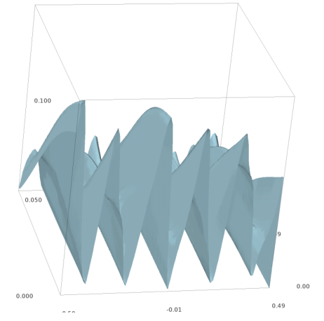
Figure 1: Absolute value of the Schottky–Igusa modular form on the 2-parameter family (6).

We now come to the Schottky Recovery Problem. Our input is a matrix $\tau$ in $\mathfrak{J}_{4}$. Our task is to compute a curve whose Riemann matrix equals $\tau$. We use the following result from Kempf’s paper [18]. The theta divisor in the Jacobian $\,\mathbb{C}^{4}/(\mathbb{Z}^{4}+\mathbb{Z}^{4}\tau)\,$ is the zero locus $\Theta^{-1}(0)$ of the Riemann theta function $\,\Theta(z):=\theta[0](\tau,z)$. For generic $\tau$ this divisor is singular at precisely two points. These represent $3$-to-$1$ maps from the curve to $\mathbb{P}^{1}$. We compute a vector $z^{*}\in\mathbb{C}^{4}$ that is a singular point of $\Theta^{-1}(0)$ by solving the system of five equations

$$\Theta(z)\,=\,\frac{\partial\Theta}{\partial z_{1}}(z)=\frac{\partial\Theta}{\partial z_{2}}(z)=\frac{\partial\Theta}{\partial z_{3}}(z)=\frac{\partial\Theta}{\partial z_{4}}(z)=0.$$ (7)

The Taylor series of the Riemann theta function $\Theta$ at the singular point $z^{*}$ has the form

$$\Theta(z^{*}+x)\,=\,f_{2}(x)\,+\,f_{3}(x)\,+\,f_{4}(x)\,+\,\,\hbox{higher order terms},$$ (8)

where $f_{s}$ is a homogeneous polynomial of degree $s$ in $x=(x_{1},x_{2},x_{3},x_{4})$.

Proposition 2.4 (Kempf [18]).

The canonical curve with Riemann matrix $\tau$ is the degree $6$ curve in $\mathbb{P}^{3}$ that is defined by the quadratic equation $f_{2}=0$ and the cubic equation $f_{3}=0$.

Thus our algorithm for the Schottky Recovery Problem consists of solving the five equations (7) for $z^{*}\in\mathbb{C}^{4}$, followed by extracting the polynomials $f_{2}$ and $f_{3}$ in the Taylor series (8). Both of these steps can be done numerically using the software abelfunctions [26].

Example 2.5.

Let $\tau\in\mathfrak{J}_{4}$ be the Riemann matrix of the genus $4$ curve $C=\{x^{3}y^{3}+x^{3}+y^{3}=1\}$. We obtain $\tau$ numerically using abelfunctions. We want to recover $C$ from $\tau$. To be precise, given only $\tau$, we want to find defining equations $f_{2}=f_{3}=0$ in $\mathbb{P}^{3}$ of the canonical embedding of $C$. For that we use evaluations of $\Theta(z)$ and its derivatives in abelfunctions, combined with a numerical optimization routine in SciPy [17]. We solve the equations (7) starting from random points $z=u+\tau v$ where $u,v\in\mathbb{R}^{4}$ with entries between $0$ and $1$. After several tries, the local method in SciPy converges to the following solution of our equations:

$$z^{*}=\bigl{(}0.55517+0.69801\textnormal{i},0.53678+0.26881\textnormal{i},-0.50000-0.58958\textnormal{i},0.55517+0.69801\textnormal{i}\bigr{)}.$$

Using (8), we computed the quadric $f_{2}$, which is nonsingular, as well as the cubic $f_{3}$:

$$\small\begin{matrix}f_{2}(x)&=&(-3.044822827+21.980542613\textnormal{i})\cdot x_{1}^{2}+(-237.95207224+252.54744634\textnormal{i})\cdot x_{1}x_{2}\\ &&\,+(-222.35552015+139.95612952\textnormal{i})\cdot x_{1}x_{3}+(-200.66932133-16.596272620\textnormal{i})\cdot x_{1}x_{4}\\ &&+(-191.16241727-85.22650070\textnormal{i})\cdot x_{2}^{2}+(-429.11449060+167.32094535\textnormal{i})\cdot x_{2}x_{3}\\ &&+(-237.952072+252.54744632\textnormal{i})\cdot x_{2}x_{4}+(-206.75896934+27.364814282\textnormal{i})\cdot x_{3}^{2}\\ &&+(222.35552013+139.95612953\textnormal{i})\cdot x_{3}x_{4}+(-3.0448227745+21.980542601\textnormal{i})\cdot x_{4}^{2}\end{matrix}$$

$$\small\begin{matrix}f_{3}(x)\quad=\quad(441.375966486+61.14097461986\textnormal{i})\cdot x_{1}^{3}+(2785.727151434+2303.609067429\textnormal{i})\cdot x_{1}^{2}x_{2}\\ +\quad\cdots\,\,\cdots\quad+\quad(441.3759668263+61.14097402189\textnormal{i})\cdot x_{4}^{3}.\end{matrix}$$

As a proof of concept we also computed the $120$ tritangent planes numerically directly from $\tau$. These planes are indexed by the $120$ odd theta characteristics $m$. In analogy to the computation in [25, §5.2] of the $28$ bitangents for $g=3$, their defining equations are

$$\frac{\partial\theta[m](\tau,z)}{\partial z_{1}}\biggl{|}_{z=0}\!\!\!\cdot\,x_{1}\,\,+\,\,\frac{\partial\theta[m](\tau,z)}{\partial z_{2}}\biggl{|}_{z=0}\!\!\!\cdot\,x_{2}\,\,+\,\,\frac{\partial\theta[m](\tau,z)}{\partial z_{3}}\biggl{|}_{z=0}\!\!\!\cdot\,x_{3}\,\,+\,\,\frac{\partial\theta[m](\tau,z)}{\partial z_{4}}\biggl{|}_{z=0}\!\!\!\cdot\,x_{4}\,\,\,=\,\,\,0.$$

We verified numerically that each such plane meets $\{f_{2}=f_{3}=0\}$ in three double points.

Remark 2.6.

On our website (2), we offer a program in Sage whose input is a symmetric $4\times 4$-matrix $\tau\in\mathfrak{H}_{4}$, given numerically. The code decides whether $\tau$ lies in $\mathfrak{J}_{4}$ and, in the affirmative case, it computes the canonical curve $\{f_{2}=f_{3}=0\}$ and its 120 tritangent planes.

3 The Tropical Schottky Problem

Curves, their Jacobians, and the Schottky locus have natural counterparts in the combinatorial setting of tropical geometry. We review the basics from [2, 3, 4, 20]. The role of a curve is played by a connected metric graph $\Gamma=(V,E,l,w)$. This has vertex set $V$, edge set $E$, a length function $l:E\rightarrow\mathbb{R}_{>0}$, and a weight function $w:V\rightarrow\mathbb{Z}_{\geq 0}$. The genus of $\Gamma$ is

$$g\,\,=\,\,|E|-|V|+1\,+\,\sum_{v\in V}w(v).$$ (9)

The moduli space $\mathcal{M}_{g}^{\rm trop}$ comprises all metric graphs of genus $g$. This is a stacky fan of dimension $3g-3$. See [4, Figure 4] for a colorful illustration. The tropical Torelli map $\,\mathcal{M}_{g}^{\rm trop}\rightarrow\mathfrak{H}_{g}^{\rm trop}\,$ takes $\Gamma$ to its (symmetric and positive semidefinite) Riemann matrix $Q_{\Gamma}$.

Fix a basis for the integral homology $H_{1}(\Gamma,\mathbb{Z})\simeq\mathbb{Z}^{g}$. Beside the usual cycles in $\Gamma$, this group has $w(v)$ generators for the virtual cycles at each vertex $v$. Let $B$ denote the $g\times|E|$ matrix whose columns record the coefficients of each edge in the basis vectors. Let $D$ be the $|E|\times|E|$ diagonal matrix whose entries are the edge lengths. The Riemann matrix of $\Gamma$ is

$$Q_{\Gamma}\,\,=\,\,B\cdot D\cdot B^{t}.$$ (10)

One way to choose a basis is to fix an orientation and a spanning tree of $\Gamma$. Each edge not in that tree then determines a cycle with $\pm 1$-coefficients. See [2, §4] for details and an example. Changing the basis of $H_{1}(\Gamma,\mathbb{Z})$ corresponds to the action of ${\rm GL}_{g}(\mathbb{Z})$ on $Q_{\Gamma}$ by conjugation.

The matrix $Q_{\Gamma}$ has rank $g-\sum_{v\in V}w(v)$. We defined $\mathfrak{H}_{g}^{\rm trop}$ with positive definite matrices. Those have rank $g$. For that reason, we now restrict to graphs with zero weights, i.e. $w\equiv 0$.

The tropical Schottky locus $\mathfrak{J}_{g}^{\rm trop}$ is the set of all matrices (10), where $\Gamma=(V,E,l)$ runs over graphs of genus $g$, and $B$ runs over their cycle bases. This set is known as the cographic locus in $\mathfrak{H}_{g}^{\rm trop}$, because the $g\times|E|$ matrix $B$ is a representation of the cographic matroid of $\Gamma$.

The Schottky Decision Problem asks for a test of membership in $\mathfrak{J}_{g}^{\rm trop}$. To be precise, given a positive definite matrix $Q$, does there exist a metric graph $\Gamma$ such that $Q=Q_{\Gamma}$?

To address this question, we need the polyhedral fan structures on $\mathfrak{J}_{g}^{\rm trop}$ and $\mathfrak{H}_{g}^{\rm trop}$. Let $G=(V,E)$ be the graph underlying $\Gamma$, with $E=\{e_{1},e_{2},\ldots,e_{m}\}$. Fix a cycle basis as above. Let $b_{1},b_{2},\ldots,b_{m}$ be the column vectors of the $g\times m$-matrix $B$. Formula (10) is equivalent to

$$Q_{\Gamma}\,\,=\,\,l(e_{1})b_{1}b_{1}^{t}+l(e_{2})b_{2}b_{2}^{t}+\cdots+l(e_{m})b_{m}b_{m}^{t}.$$ (11)

The cone of all Riemann matrices for the graph $G$, allowing the edge lengths to vary, is

$$\sigma_{G,B}\,\,=\,\,\mathbb{R}_{>0}\bigl{\{}b_{1}b_{1}^{t},\,b_{2}b_{2}^{t},\,\ldots\,,\,b_{m}b_{m}^{t}\bigr{\}}\,.$$ (12)

This is a relatively open rational convex polyhedral cone, spanned by matrices of rank $1$. The collection of all cones $\sigma_{G,B}$ is a polyhedral fan whose support is the Schottky locus $\mathfrak{J}_{g}^{\rm trop}$.

This fan is a subfan of the second Voronoi decomposition of the cone $\mathfrak{H}_{g}^{\rm trop}$ of positive definite matrices. The latter fan is defined as follows. Fix a Riemann matrix $Q\in\mathfrak{H}_{g}^{\rm trop}$ and consider its quadratic form $\,\mathbb{Z}^{g}\rightarrow\mathbb{R},\,x\mapsto x^{t}Qx$. The values of this quadratic form define a regular polyhedral subdivision of $\mathbb{R}^{g}$ with vertices at $\mathbb{Z}^{g}$. This is denoted ${\rm Del}(Q)$ and known as the Delaunay subdivision of $Q$. Dual to ${\rm Del}(Q)$ is the Voronoi decomposition of $\mathbb{R}^{g}$. The cells of the Voronoi decomposition of $Q$ are the lattice translates of the Voronoi polytope

$$\bigl{\{}\,p\in\mathbb{R}^{g}\,:\,2p^{t}Qx\leq x^{t}Qx\,\,\,\hbox{for all}\,\,x\in\mathbb{Z}^{g}\,\bigr{\}}.$$ (13)

This is the set of points in $\mathbb{R}^{g}$ for which the origin is the closest lattice point, in the norm given by $Q$. If $Q$ is generic then the Delaunay subdivision is a triangulation and the Voronoi polytope (13) is simple. It is dual to the link of the origin in the simplicial complex ${\rm Del}(Q)$.

The structures above represent principally polarized abelian varieties in tropical geometry. A tropical abelian variety is the torus $\mathbb{R}^{g}/\mathbb{Z}^{g}$ together with a quadratic form $Q\in\mathfrak{H}_{g}^{\rm trop}$. The tropical theta divisor is given by the codimension one cells in the induced Voronoi decomposition of $\mathbb{R}^{g}/\mathbb{Z}^{g}$. See [2, §5] for an introduction with many pictures and many references.

We now fix an arbitrary Delaunay subdivision $D$ of $\mathbb{R}^{g}$. Its secondary cone is defined as

$$\sigma_{D}\,\,=\,\,\bigl{\{}\,Q\in\mathfrak{H}_{g}^{\rm trop}\,\,|\,\,\operatorname{Del}(Q)=D\bigr{\}}\,.$$ (14)

This is a relatively open convex polyhedral cone. It consists of positive definite matrices $Q$ whose Voronoi polytopes (13) have the same normal fan. The group ${\rm GL}_{g}(\mathbb{Z})$ acts on the set of secondary cones. In his classical reduction theory for quadratic forms, Voronoi [29] proved that the cones $\sigma_{D}$ form a polyhedral fan, now known as the second Voronoi decomposition of $\mathfrak{H}_{g}^{\rm trop}$, and that there are only finitely many secondary cones $\sigma_{D}$ up to the action of ${\rm GL}_{g}(\mathbb{Z})$. The following summarizes characteristic features for matrices in the Schottky locus $\mathfrak{J}_{g}^{\rm trop}$.

Proposition 3.1.

Fix a graph $G$ with metric $D$, homology basis $B$, and Riemann matrix $Q=BDB^{t}$. The Voronoi polytope (13) is affinely isomorphic to the zonotope $\sum_{i=1}^{m}[-b_{i},b_{i}]$. The secondary cone $\sigma_{{\rm Del}(Q)}$ is spanned by the rank one matrices $b_{i}b_{i}^{t}$: it equals $\sigma_{G,B}$ in (12).

Proof.

This can be extracted from Vallentin’s thesis [28]. The affine isomorphism is given by the invertible matrix $Q$, as explained in item iii) of [28, §3.3.1]. The Voronoi polytope being the zonotope $\sum_{i=1}^{m}[-b_{i},b_{i}]$ follows from the discussion on cographic lattices in [28, §3.5]. The result for the secondary cone is derived from [28, §2.6]. See [28, §4] for many examples. ∎

We now fix $g=4$. Vallentin [28, §4.4.6] lists all $52$ combinatorial types of Delaunay subdivisions of $\mathbb{Z}^{4}$. His table contains the f-vectors of all $52$ Voronoi polytopes. Precisely $16$ of these types are cographic, and these comprise the Schottky locus $\mathfrak{J}_{4}^{\rm trop}$. These are described in rows 3 to 18 of the table in [28, §4.4.6]. We reproduce the relevant data in Table LABEL:table-trop-schottky. The following key lemma is found by inspecting Vallentin’s list of f-vectors.

Lemma 3.2.

The f-vectors of the $16$ Voronoi polytopes representing the Schottky locus $\mathfrak{J}_{4}^{\rm trop}$ are distinct from the f-vectors of the other $36$ Voronoi polytopes, corresponding to $\mathfrak{H}_{4}^{\rm trop}\backslash\mathfrak{J}_{4}^{\rm trop}$.

This lemma gives rise to the following method for the tropical Schottky decision problem.

Algorithm 3.3 (Tropical Schottky Decision).

Input: $Q\in\mathfrak{H}_{4}^{\rm trop}\!$. Output: Yes, if $\,Q\in\mathfrak{J}_{4}^{\rm trop}\!$.
1. Compute the Voronoi polytope in (13) for the quadratic form $Q$.
2. Determine the f-vector $(f_{0},f_{1},f_{2},f_{3})$ of this $4$-dimensional polytope.
3. Check whether this f-vector appears in our Table LABEL:table-trop-schottky. Output “Yes” if this holds.

Table 1: The tropical Schottky locus for $g=4$

Graph $G$	Riemann matrix $Q_{\Gamma}$	$f_{0}$	$f_{1}$	$f_{2}$	$f_{3}$	Dimension of $\sigma_{D}$
	$\begin{pmatrix}3&1&-1&0\\ 1&4&1&1\\ -1&1&4&-1\\ 0&1&-1&3\end{pmatrix}$	96	198	130	28	9
	$\begin{pmatrix}4&2&-2&-1\\ 2&4&-1&-2\\ -2&-1&4&2\\ -1&-2&2&4\end{pmatrix}$	102	216	144	30	9
	$\begin{pmatrix}2&0&-1&0\\ 0&3&1&1\\ -1&1&4&-1\\ 0&1&-1&3\end{pmatrix}$	72	150	102	24	8
	$\begin{pmatrix}3&2&1&-1\\ 2&4&2&-1\\ 1&2&4&1\\ -1&-1&1&3\end{pmatrix}$	78	168	116	26	8
	$\begin{pmatrix}3&1&-1&-1\\ 1&3&1&1\\ -1&1&3&2\\ -1&1&2&3\end{pmatrix}$	60	134	98	24	7
	$\begin{pmatrix}2&0&-1&-1\\ 0&2&-1&-1\\ -1&-1&4&3\\ -1&-1&3&4\end{pmatrix}$	54	116	84	22	7
	$\begin{pmatrix}2&0&-1&0\\ 0&2&0&-1\\ -1&0&3&1\\ 0&-1&1&3\end{pmatrix}$	54	114	80	20	7
	$\begin{pmatrix}3&1&-1&0\\ 1&3&1&0\\ -1&1&3&0\\ 0&0&0&1\end{pmatrix}$	48	96	64	16	7
	$\begin{pmatrix}2&0&-1&-1\\ 0&2&1&1\\ -1&1&3&2\\ -1&1&2&3\end{pmatrix}$	46	108	84	22	6
	$\begin{pmatrix}2&-1&-1&-1\\ -1&3&2&2\\ -1&2&3&2\\ -1&2&2&3\end{pmatrix}$	42	94	72	20	6
	$\begin{pmatrix}2&1&1&0\\ 1&3&2&0\\ 1&2&3&0\\ 0&0&0&1\end{pmatrix}$	36	74	52	14	6
	$\begin{pmatrix}2&1&0&0\\ 1&2&0&0\\ 0&0&2&1\\ 0&0&1&2\end{pmatrix}$	36	72	48	12	6
	$\begin{pmatrix}2&1&1&1\\ 1&2&1&1\\ 1&1&2&1\\ 1&1&1&2\end{pmatrix}$	30	70	60	20	5
	$\begin{pmatrix}2&1&1&0\\ 1&2&1&0\\ 1&1&2&0\\ 0&0&0&1\end{pmatrix}$	28	62	48	14	5
	$\begin{pmatrix}2&1&0&0\\ 1&2&0&0\\ 0&0&1&0\\ 0&0&0&1\end{pmatrix}$	24	48	34	10	5
	$\begin{pmatrix}1&0&0&0\\ 0&1&0&0\\ 0&0&1&0\\ 0&0&0&1\end{pmatrix}$	16	32	24	8	4

We implemented Algorithm 3.3 using existing software for polyhedral geometry, namely the GAP package polyhedral due to Dutour Sikirić [8, 9], as well as Joswig’s polymake [10].

The first column of Table LABEL:table-trop-schottky shows all relevant graphs $G$ of genus $4$. The second column gives a representative Riemann matrix. Here all edges have length $1$ and a cycle basis $B$ was chosen. Using (12), we also precomputed the secondary cones $\sigma_{G,B}$ for the $16$ representatives.

Example 3.4.

Using the GAP package polyhedral [8] we compute the Voronoi polytope of

$$\small Q\,\,=\,\,\begin{pmatrix}14&-9&11&0\\ -9&11&-2&1\\ 11&-2&21&11\\ 0&1&11&14\end{pmatrix}.$$

Its $f$-vector is $(62,142,104,24)$. This does not appear in Table LABEL:table-trop-schottky. Hence $Q$ is not in $\mathfrak{J}_{4}^{\rm trop}$.

We now address the Schottky Recovery Problem. The input is a matrix $Q\in\mathfrak{J}_{4}^{\rm trop}$. From Algorithm 3.3 we know the f-vector of the Voronoi polytope. Using Table LABEL:table-trop-schottky, this uniquely identifies the graph $G$. Note that our graphs $G$ are dual to those in [28, §4.4.4]. From our precomputed list, we also know the secondary cone $\sigma_{G,B}$ for some choice of basis $B$.

Algorithm 3.5 (Tropical Schottky Recovery).

Input: $Q\in\mathfrak{J}_{4}^{\rm trop}$.
Output: A metric graph $\Gamma$ whose Riemann matrix $Q_{\Gamma}$ equals $Q$.
1. Identify the underlying graph $G$ from Table LABEL:table-trop-schottky. Retrieve the basis $B$ and the cone $\sigma_{G,B}$.
2. Let $D={\rm Del}(Q)$ and compute the secondary cone $\sigma_{D}$ as in (14).
3. The cones $\sigma_{D}$ and $\sigma_{G,B}$ are related by a linear transformation $X\in{\rm GL}_{4}(\mathbb{Z})$. Compute $X$.
4. The matrix $X^{t}QX$ lies in $\sigma_{G,B}$. Compute $\ell_{1},\ldots,\ell_{m}$ such that $X^{t}QX=\sum_{i=1}^{m}\ell_{i}b_{i}b_{i}^{t}$.
5. Output the graph $G$ with length $\ell_{i}$ for its $i$-th edge, corresponding to the column $b_{i}$ of $B$.

We implemented this algorithm as follows. Step 2 can be done using polyhedral [8]. This code computes the secondary cone $\sigma_{D}$ containing a given positive definite matrix $Q$. The matrix $X\in{\rm GL}_{4}(\mathbb{Z})$ in Step 3 is also found by polyhedral, but with external calls to the package isom due to Plesken and Souvignier [22]. We refer to [9, §4] for details. For Step 4 we note that the rank $1$ matrices $b_{1}b_{1}^{t},\ldots,b_{m}b_{m}^{t}$ are linearly independent [28, §4.4.4]. Indeed, the two $9$-dimensional secondary cones $\sigma_{G,B}$ at the top of Table LABEL:table-trop-schottky are simplicial, and so are their faces. Hence the multipliers $\ell_{1},\ldots,\ell_{m}$ found in Step 4 are unique and positive. These $\ell_{i}$ must agree with the desired edge lengths $l(e_{i})$, by the formula for $Q=Q_{\Gamma}$ in (11).

Example 3.6.

Consider the Schottky Recovery Problem for the matrix

$$\small Q\,\,=\,\,\begin{pmatrix}17&5&3&5\\ 5&19&7&11\\ 3&7&23&16\\ 5&11&16&29\end{pmatrix}.$$ (15)

Using polyhedral, we find that the f-vector of its Voronoi polytope is $(96,198,130,28)$. This matches the first row in Table LABEL:table-trop-schottky. Hence $Q\in\mathfrak{J}_{4}^{\rm trop}$, and $G$ is the triangular prism. Using polyhedral and isom, we find a matrix that maps $Q$ into our preprocessed secondary cone:

$$\small X=\begin{pmatrix}0&0&0&1\\ 1&0&0&0\\ 0&1&1&0\\ -1&-1&0&0\end{pmatrix}\,\in\,{\rm GL}_{4}(\mathbb{Z})\qquad\hbox{gives}\qquad Q^{\prime}=X^{t}QX=\begin{pmatrix}26&9&-9&0\\ 9&20&7&-2\\ -9&7&23&3\\ 0&-2&3&17\end{pmatrix}\,\in\,\sigma_{G,B}.$$

This $Q^{\prime}$ is the Riemann matrix of the metric graph in Figure 2, with basis cycles $e_{2}+e_{6}-e_{3}$, $-e_{1}-e_{4}+e_{7}+e_{2}$, $-e_{1}-e_{5}+e_{8}+e_{3}$, and $e_{4}+e_{9}-e_{5}$. These are the rows of the $4\times 9$-matrix $B$. In Step 4 of Algorithm 3.5 we compute $D={\rm diag}(\ell_{1},\ldots,\ell_{9})={\rm diag}(7,9,9,2,3,8,2,4,12)$. In Step 5 we output the metric graph in Figure 2. Its Riemann matrix equals $Q=BDB^{t}$.

Figure 2: Metric graph with edge lengths in red. Its Riemann matrix matches (15).

It is instructive to compare Algorithms 3.3 and 3.5 with Section 2. Our classical solution is not just the abstract Riemann surface but it consists of a canonical embedding into $\mathbb{P}^{3}$.

Canonical embeddings also exist for metric graphs $\Gamma$, as explained in [14, §7]. However, even computing the ambient space $|K|$, that plays the role of $\mathbb{P}^{3}$, is non-trivial in that setting. For $g=4$ this is solved in [19]. An alternative approach is to construct a classical curve over a non-archimedean field that tropicalizes to $\Gamma$. See [2, §7.3] for first steps in that direction.

Example 2.3 explored the Schottky locus in a two-parameter family of Riemann matrices. In the tropical setting, it is natural to intersect $\mathfrak{H}_{g}^{\rm trop}$ with an affine-linear space $L$ of symmetric matrices. The intersection $\mathfrak{H}_{g}^{\rm trop}\cap L$ is a spectrahedron. By the Schottky locus of a spectrahedron we mean $\mathfrak{J}_{g}^{\rm trop}\cap L$. This is an infinite periodic polyhedral complex inside the spectrahedron. For quartic spectrahedra [21], when $g=4$, this locus has codimension one.

Example 3.7 (The Schottky locus of a quartic spectrahedron).

We consider the matrix

$$\small\!Q=\begin{bmatrix}1589-2922s+960t&789-1322s&-820+660s-1350t&\!\!-820+3260s+2550t\\ 789-1322s&1589-2922s-960t\!&\!\!\!-820+3260s-2550t\!&-820+660s+1350t\\ -820+660s-1350t&\!-820+3260s-2550t\!&1665+450s+3120t&-25-2930s\\ \!-820+3260s+2550t&-820+660s+1350t&-25-2930s&1665+450s-3120t\end{bmatrix}\!.$$

Here $s$ and $t$ are parameters. This defines a plane $L$ in the space of symmetric $4\times 4$-matrices. The left diagram in Figure 3 shows the hyperbolic curve $\{{\rm det}(Q)=0\}$. The spectrahedron $\mathfrak{H}_{g}^{\rm trop}\cap L$ is bounded by its inner oval. The right diagram shows the second Voronoi decomposition. The Schottky locus $\mathfrak{J}_{g}^{\rm trop}\cap L$ is a proper subgraph of its edge graph. It is shown in red. Note that the graph has infinitely many edges and regions.

Remark 3.8.

We described some computations in GAP and in polymake that realize Algorithms 3.3 and 3.5. The code for these implementations is made available on our website (2).

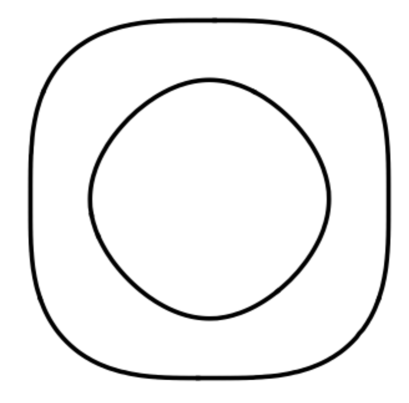
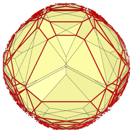
Figure 3: A quartic spectrahedron (left) and its second Voronoi decomposition (right). The Schottky locus of that spectrahedron consists of those edges that are highlighted in red.

4 Tropical Meets Classical

In this section we present a second solution to the tropical Schottky problem. It is new and different from the one in Section 3, and it links directly to the classical solution in Section 2.

Let $Q\in\mathfrak{H}_{g}^{\rm trop}$ be a positive definite matrix for arbitrary $g$. Mikhalkin and Zharkov [20, §5.2] define the following analogue to the Riemann theta function in the max-plus algebra:

$$\Theta(Q,x)\,\,:=\,\,\max_{\lambda\in\mathbb{Z}^{g}}\{\lambda^{t}Qx-\frac{1}{2}\lambda^{t}Q\lambda\}.$$ (16)

This tropical theta function describes the asymptotic behavior of the classical Riemann theta function with Riemann matrix $t\cdot\tau$ when $t$ goes to infinity, as long as there are no cancellations. This is made precise in Proposition 4.6. Here, the real matrix $Q$ is the imaginary part of $\tau$.

Analogously, for $u\in\mathbb{Z}^{g}$, we define the tropical theta constant with characteristic $u$ to be

$$\Theta_{u}(Q)\,\,:=\,\,2\cdot\Theta(Q,\frac{u}{2})-\frac{1}{4}u^{t}Qu.$$ (17)

In the classical case, characteristics are vectors $m=(m^{\prime},m^{\prime\prime})$ in $\mathbb{Z}^{2g}$. But, only $u=m^{\prime}$ contributes to the aforementioned asymptotics. Note that $\Theta_{u}(Q)$ depends only on $u$ modulo $2$.

Definition 4.1.

For any $v\in\mathbb{Z}^{g}$ consider the following signed sum of tropical theta constants:

$$\vartheta_{v}(Q)\,\,\,:=\sum_{u\in(\mathbb{Z}/2\mathbb{Z})^{g}}\!\!(-1)^{u^{t}v}\cdot\Theta_{u}(Q).$$ (18)

The theta matroid $M(Q)$ is the binary matroid represented by the collection of vectors

$$\bigl{\{}v\in(\mathbb{Z}/2\mathbb{Z})^{g}:\,\vartheta_{v}(Q)\neq 0\bigr{\}}.$$ (19)

The tropical theta constants and the theta matroid are invariant under basis changes $S\in\textnormal{GL}_{g}(\mathbb{Z})$. We have $\,\vartheta_{u}(Q)=\vartheta_{S^{-1}u}(S^{t}QS)\,$ for all $u\in\mathbb{Z}^{g}$, and therefore $M(Q)=M(S^{t}QS)$.

Here is the promised new approach to the Schottky problem. If $Q$ lies in the tropical Schottky locus then $M(Q)$ is the desired cographic matroid and (18) furnishes edge lengths.

Theorem 4.2.

If $\,Q\in\mathfrak{J}_{g}^{\rm trop}$ then the matroid $M(Q)$ is cographic. In that graph, we assign the length $\,2^{3-g}\cdot\vartheta_{v}(Q)\,$ to the edge labeled $v$. The resulting metric graph has Riemann matrix $Q$.

This says, in particular, that $\vartheta_{v}(Q)$ is non-negative when $Q$ comes from a metric graph.

Proof.

Since $Q\in\mathfrak{J}_{g}^{\rm trop}$, there exists a unimodular matrix $B=(b_{1},\ldots,b_{m})\in\{-1,0,+1\}^{g\times m}$ and a diagonal matrix $D={\rm diag}(\ell_{1},\ldots,\ell_{m})$ such that $Q=BDB^{t}=\sum_{i=1}^{m}\ell_{i}b_{i}b_{i}^{t}$. We claim

$$\Theta_{u}(Q)\,\,=\,\,-\,\frac{1}{4}\,\cdot\!\sum_{b_{i}^{t}u\textnormal{ is odd}}\!\!\ \ell_{i}\qquad\quad\hbox{for all $\,u\in\mathbb{Z}^{g}$}.$$ (20)

Here the $\ell_{i}$ are positive real numbers. First, we note that

$$\Theta_{u}(Q)\,\,=\,\,\max_{\lambda\in\mathbb{Z}^{g}}\,\bigl{\{}-(\lambda+\frac{u}{2})^{t}Q(\lambda+\frac{u}{2})\,\bigr{\}}\,\,\,\leq\,\,\,\sum_{i=1}^{m}-\ell_{i}\cdot\min_{\lambda\in\mathbb{Z}^{g}}\biggl{\{}\bigl{(}\,b_{i}^{t}\cdot(\lambda+\frac{u}{2})\,\bigr{)}^{2}\biggr{\}}.$$

If $\,b_{i}^{t}u\,$ is even, then $b_{i}^{t}\cdot(\lambda+\frac{u}{2})=0$ for some $\lambda\in\mathbb{Z}^{g}$. Otherwise, the absolute value of $b_{i}^{t}\cdot(\lambda+\frac{u}{2})$ is at least $1/2$. This shows that $\Theta_{u}(Q)\leq-\frac{1}{4}\cdot\sum_{b_{i}^{t}u\textnormal{ is odd}}\ell_{i}$. To derive the reverse inequality, let $\,I=\bigl{\{}i\,:\,u_{i}\,\hbox{is odd}\bigr{\}}\subset\{1,\ldots,g\}$. By a result of Ghouila-Houri [11] on unimodular matrices, we can find $w\in\mathbb{Z}^{g}$ with $w_{i}=\pm 1$ if $i\in I$ and $w_{i}=0$ otherwise, such that $b_{i}^{t}\cdot w\in\{0,\pm 1\}$ for all $1\leq i\leq m$. The vector $\lambda_{0}=\frac{1}{2}(w-u)$ lies in $\mathbb{Z}^{g}$. One checks that

$$-(\lambda_{0}+\frac{u}{2})^{t}Q(\lambda_{0}+\frac{u}{2})\,=\,\sum_{i=1}^{m}-\ell_{i}\cdot(b_{i}^{t}\cdot(\lambda_{0}+\frac{u}{2}))^{2}\,=\,-\frac{1}{4}\sum_{i=1}^{m}\ell_{i}\cdot(b_{i}^{t}\cdot w)^{2}\,=\,-\frac{1}{4}\cdot\sum_{b_{i}^{t}u\textnormal{ is odd}}\!\!\ell_{i}.$$

Therefore, we also have $\,\Theta_{u}(Q)\geq-\frac{1}{4}\cdot\sum_{b_{i}^{t}u\textnormal{ is odd}}\ell_{i}$. This establishes the assertion in (20).

We next claim that, under the same hypotheses as above, the function in (18) satisfies

$$\vartheta_{v}(Q)\,\,=\,\,\,2^{g-3}\!\sum_{b_{i}\equiv v\,{\rm mod}\,2}\!\!\ell_{i}\qquad\hbox{for all}\,\,v\in\mathbb{Z}^{g}.$$ (21)

Indeed, substituting the right hand side of (20) for $\Theta_{u}(Q)$ into (18), we find that

$$\vartheta_{v}(Q)\,\,=\,\,-\frac{1}{4}\cdot\sum_{u\in(\mathbb{Z}/2\mathbb{Z})^{g}}\sum_{b_{i}^{t}u\textnormal{ is odd}}(-1)^{u^{t}v}\cdot\ell_{i}\,\,=\,\,-\frac{1}{4}\cdot\sum_{i=1}^{m}\ell_{i}\cdot(|E_{i}|-|O_{i}|),$$

where $E_{i}=\{u\in(\mathbb{Z}/2\mathbb{Z})^{g}:b_{i}^{t}u\,\,{\rm odd},\,u^{t}v\,\,{\rm even}\}$ and $O_{i}=\{u\in(\mathbb{Z}/2\mathbb{Z})^{g}:b_{i}^{t}u\,\,{\rm odd},\,u^{t}v\,\,{\rm odd}\}$. If $b_{i}\equiv v\,{\rm mod}\,2$ then $E_{i}=\emptyset$ and $|O_{i}|=2^{g-1}$. Otherwise, $|E_{i}|=|O_{i}|=2^{g-2}$. This proves (21).

Since $Q\in\mathfrak{J}_{g}^{\rm trop}$, this matrix comes from a graph $G$. We may assume that $G$ has no $2$-valent vertices. This ensures that any pair is independent in the cographic matroid of $G$.

The column $b_{i}$ of the matrix $B$ records the coefficients of the $i$-th edge in a cycle basis of the graph $G$. The residue class of $b_{i}$ modulo $2$ is unique. For $v\in\mathbb{Z}^{g}$ with $b_{i}\equiv v\,{\rm mod}\,2$, the sum in (21) has only term $\ell_{i}$, and we have $\ell_{i}=2^{3-g}\vartheta_{v}(Q)$. If $v\in\mathbb{Z}^{g}$ is not congruent to $b_{i}$ for any $i$ then $\vartheta_{v}(Q)=0$. This proves that the theta matroid $M(Q)$ equals the cographic matroid of $G$, and the edge lengths $\ell_{i}$ are recovered from $Q$ by the rule in Theorem 4.2. ∎

By Theorem 4.2, the non-negativity of $\vartheta_{v}(Q)$ is a necessary condition for $Q$ to be in $\mathfrak{J}_{g}^{\rm trop}$.

Example 4.3.

For the matrix $Q$ in Example 3.4, we find $\vartheta_{0001}(Q)=-\frac{1}{2}$. Hence $\,Q\not\in\mathfrak{J}_{4}^{\rm trop}$.

This necessary (but not sufficient) condition translates into the following algorithm:

Algorithm 4.4 (Tropical Schottky Recovery).

Input: $Q\in\mathfrak{J}_{g}^{\rm trop}$.
Output: A metric graph $\Gamma$ whose Riemann matrix $Q_{\Gamma}$ equals $Q$.
1. Compute the theta matroid $M(Q)$. It is cographic and determines a unique graph $G$.
2. Compute all edge lengths using the formula $\ell_{i}=2^{3-g}\vartheta_{v}(Q)$. Set $\,D={\rm diag}(\ell_{1},\ldots,\ell_{m})$.
3. Output the metric graph $(G,D)$.
4. (Optional) As in Algorithm 3.5, find a basis $B$ such that $BDB^{t}=Q$.

Example 4.5.

Let $Q$ be the matrix in Example 3.6. For each $u\in(\mathbb{Z}/2\mathbb{Z})^{4}$, we list the theta constant $\Theta_{u}(Q)$, the weight $2^{-1}\vartheta_{u}(Q)$ and the label of the corresponding edge in Figure 2:

$$\small\setcounter{MaxMatrixCols}{16}\begin{matrix}u&\!0001\!&\!0010\!&\!0011\!&\!0100\!&\!0101\!&\!0110\!&\!0111\!&\!1000\!&\!1001\!&\!1010\!&\!1011\!&\!1100\!&\!1101\!&\!1110\!&\!1111\vskip 3.0pt plus 1.0pt minus 1.0pt\\ -\Theta_{u}&\frac{29}{4}&\frac{23}{4}&5&\frac{19}{4}&\frac{13}{2}&7&\frac{31}{4}&\frac{17}{4}&9&\frac{17}{2}&\frac{33}{4}&\frac{13}{2}&\frac{43}{4}&\frac{41}{4}&\frac{21}{2}\vskip 3.0pt plus 1.0pt minus 1.0pt\\ 2^{-1}\vartheta_{u}&9&7&9&8&2&0&4&12&0&0&0&0&2&0&3\\ {\rm Edge}&e_{2}&e_{1}&e_{3}&e_{6}&e_{7}&-&e_{8}&e_{9}&-&-&-&-&e_{4}&-&e_{5}\\ \end{matrix}$$

We now explain the connection between the classical and tropical theta functions. In particular, we will show how the process of tropicalization relates Theorems 2.1 and 4.2.

In order to tropicalize the Schottky–Igusa modular form, we must study the order of growth of the theta constants when the entries of the Riemann matrix grow. This information is captured by the tropical theta constants. The following proposition makes that precise.

Proposition 4.6.

Fix $Q\in\mathfrak{H}_{g}^{\rm trop}$, and let $P(t)$ be any real symmetric $g\times g$-matrix that depends on a parameter $t\in\mathbb{R}$. For every $m\in(\mathbb{Z}/2\mathbb{Z})^{2g}$ there is a constant $C\in\mathbb{R}$ such that

$$0\,\,\leq\,\,\frac{|\,\theta[m](P(t)+t\cdot\textnormal{i}Q,0)\,|}{|\,\exp(t\cdot\pi\cdot\Theta_{m^{\prime}}(Q))\,|}\leq\,\,C\,\,\quad\hbox{for all $\,t\geq 0$}.$$ (22)

Moreover, we can choose $P(t)$ such that the ratio above does not approach zero for $t\to\infty$.

Here $\theta[m](\tau,0)$ is the classical theta constant from (3), and $\Theta_{m^{\prime}}(Q)$ is the tropical theta constant defined in (17). We use the notation $m=(m^{\prime},m^{\prime\prime})$ for vectors in $\mathbb{Z}^{2g}$ as in Section 2.

Proof.

Consider the lattice points $\lambda$ where the maximum in (16) for $x=m^{\prime}/2$ is attained. The corresponding summands in (3) with $\lambda=n$ have the same asymptotic behavior as $\exp(t\cdot\pi\Theta_{m^{\prime}}(Q))$ for $t\to\infty$. The sum over the remaining exponentials tends to zero since it can be bounded by a sum of finitely many Gaussian integrals with variance going to zero for $t\to\infty$. We can choose the real symmetric matrix $P(t)$ in such a way that no cancellation of highest order terms happens. Then the expression in (22) is bounded away from zero. ∎

Remark 4.7.

On the Siegel upper-half space $\mathfrak{H}_{g}$ we have an action by the symplectic group $\textnormal{Sp}_{2g}(\mathbb{Z})$. Two matrices from the same orbit under this action correspond to the same abelian variety. However their tropicalizations may vary drastically. Consider for example the case $g=1$: $\begin{pmatrix}0&-1\\ 1&k\end{pmatrix}\in\textnormal{Sp}_{2}(\mathbb{Z})$ sends $\tau=\textnormal{i}$ to a complex number with imaginary part $\frac{1}{1+k^{2}}$.

We now assume that $g=4$. For any subset $M\subset(\mathbb{Z}/2\mathbb{Z})^{8}$ we write $M^{\prime}=\{m^{\prime}:\,m\in M\}$ and similarly for $M^{\prime\prime}$. The following lemma concerns the possible choices for Theorem 2.1.

Lemma 4.8.

For any azygetic triple $\{m_{1},m_{2},m_{3}\}$ and any matching subgroup $N\subset(\mathbb{Z}/2\mathbb{Z})^{8}$,

• there exist indices $1\leq i<j\leq 3$ such that $(m_{i}+N)^{\prime}=(m_{j}+N)^{\prime}$, and

• if $\dim N^{\prime}=3$ and $(m_{1}+N)^{\prime}=(m_{2}+N)^{\prime}\neq(m_{3}+N)^{\prime}$, then $m_{1}^{\prime},m_{2}^{\prime}\in N^{\prime}$.

Proof.

This purely combinatorial statement can be proved by exhaustive computation. ∎

For instance, consider the specific choice of $m_{1},m_{2},m_{3},N$ made prior to Example 2.2. This has $\dim N^{\prime}=2$, and Lemma 4.8 (1) holds with $i=2$, $j=3$. If we exchange the first four coordinates with the last four coordinates, then $\dim N^{\prime}=3$, $m_{1}^{\prime},m_{3}^{\prime}\in N^{\prime}$ and $m_{2}^{\prime}\not\in N^{\prime}$.

Recall from Theorem 2.1 that a matrix $\tau\in\mathfrak{H}_{4}$ is in the Schottky locus if and only if $\pi_{1}^{2}+\pi_{2}^{2}+\pi_{3}^{2}-2(\pi_{1}\pi_{2}+\pi_{1}\pi_{3}+\pi_{2}\pi_{3})$ vanishes. The tropicalization of this expression equals

$$\max_{i,j=1,2,3}(\pi^{\textnormal{trop}}_{i}+\pi^{\textnormal{trop}}_{j}),$$ (23)

where $\pi^{\textnormal{trop}}_{i}=\sum_{m\in m_{i}+N}\Theta_{m^{\prime}}(Q)$ is the tropicalization of the product (4), with $Q={\rm im}(\tau)$.

The tropical Schottky–Igusa modular form (23) defines a piecewise-linear convex function $\mathfrak{H}_{4}^{\rm trop}\rightarrow\mathbb{R}$. Its breakpoint locus is the set of Riemann matrices $Q$ for which the maximum in (23) is attained twice. That set depends on our choice of $m_{1},m_{2},m_{3},N$. That choice is called admissible if $N\subset(\mathbb{Z}/2\mathbb{Z})^{8}$ has rank three, the triple $\{m_{1},m_{2},m_{3}\}\subset(\mathbb{Z}/2\mathbb{Z})^{8}$ is azygetic, all elements of $m_{i}+N$ are even, and the group $N^{\prime}\subset(\mathbb{Z}/2\mathbb{Z})^{4}$ also has rank three. We define the tropical Igusa locus in $\mathfrak{H}_{g}^{\rm trop}$ to be the intersection, over all admissible choices $m_{1},m_{2},m_{3},N$, of the breakpoint loci of the tropical modular forms $(\ref{eq:tropicalschottkyigusa})$.

Theorem 4.9.

A matrix $Q\in\mathfrak{H}_{4}^{\rm trop}$ lies in the tropical Igusa locus if and only if $\vartheta_{v}(Q)\geq 0$ for all $v\in\mathbb{Z}^{4}$. That locus contains the tropical Schottky locus $\mathfrak{J}_{4}^{\rm trop}\!$, but they are not equal.

Proof.

We are interested in how the maximum in (23) is attained. By Lemma 4.8 (1), after relabeling, $\,\pi^{\textnormal{trop}}_{1}=\pi^{\textnormal{trop}}_{2}$. The maximum is attained twice if and only if $\pi^{\textnormal{trop}}_{1}\geq\pi^{\textnormal{trop}}_{3}$. By Lemma 4.8 (2), this is equivalent to

$$\sum_{u\in N^{\prime}}\Theta_{u}(Q)\,\,\geq\,\,\sum_{u\not\in N^{\prime}}\Theta_{u}(Q).$$ (24)

Let $v$ be the non-zero vector in $(\mathbb{Z}/2\mathbb{Z})^{4}$ that is orthogonal to $N^{\prime}$. Then (24) is equivalent to

$$\vartheta_{v}(Q)\,\,\,=\sum_{u\in(\mathbb{Z}/2\mathbb{Z})^{4}}\!\!(-1)^{u^{t}v}\Theta_{u}(Q)\,\,\,\geq\,\,\,0.$$

This proves the first assertion, if we knew that every $v$ arises from some admissible choice.

We saw in Theorem 4.2 that $\vartheta_{v}(Q)\geq 0$ for all $v$ whenever $Q\in\mathfrak{J}_{4}^{\rm trop}$. Hence the tropical Schottky locus $\mathfrak{J}_{4}^{\rm trop}$ is contained in the tropical Igusa locus. The two loci are not equal because the latter contains the zonotopal locus of $\mathfrak{H}_{4}^{\rm trop}$. This consists of matrices $Q=BDB^{t}$ where $B$ represents any unimodular matroid, not necessarily cographic. By [28, §4.4.4], the second Voronoi decomposition of $\mathfrak{H}_{4}^{\rm trop}$ has a non-cographic $9$-dimensional cone in its zonotopal locus. It is unique modulo ${\rm GL}_{4}(\mathbb{Z})$. We verified that all $16$ tropical modular forms $\vartheta_{v}$ are non-negative on that cone. This establishes the last assertion in Theorem 4.9.

To finish the proof, we still need that every $v\in(\mathbb{Z}/2\mathbb{Z})^{4}\backslash\{0\}$ is orthogonal to $N^{\prime}$ for some admissible choice $m_{1},m_{2},m_{3},N$. By permuting coordinates, it suffices to show this for

$$v\,\in\,\{(1,0,0,0)^{t},(1,1,0,0)^{t},(1,1,1,0)^{t},(1,1,1,1)^{t}\}.$$

For $v=(1,0,0,0)^{t}$ we take

$$\small m_{1}=\begin{pmatrix}0&1\\ 0&0\\ 0&0\\ 0&1\end{pmatrix}\!,\,m_{2}=\begin{pmatrix}1&1\\ 1&0\\ 1&1\\ 0&1\end{pmatrix}\!,\,m_{3}=\begin{pmatrix}0&1\\ 0&0\\ 1&0\\ 1&0\end{pmatrix}\!,\,\,n_{1}=\begin{pmatrix}0&1\\ 1&0\\ 0&1\\ 0&1\end{pmatrix}\!,\,n_{2}=\begin{pmatrix}0&1\\ 0&0\\ 1&0\\ 1&1\end{pmatrix}\!,\,n_{3}=\begin{pmatrix}0&0\\ 0&1\\ 1&0\\ 0&0\end{pmatrix}\!.$$

For $v=(1,1,0,0)^{t}$ we take

$$\small m_{1}=\begin{pmatrix}0&1\\ 0&0\\ 0&0\\ 0&1\end{pmatrix}\!,\,m_{2}=\begin{pmatrix}1&1\\ 1&0\\ 1&1\\ 0&0\end{pmatrix}\!,\,m_{3}=\begin{pmatrix}1&0\\ 0&0\\ 0&0\\ 0&1\end{pmatrix}\!,\,\,n_{1}=\begin{pmatrix}1&1\\ 1&1\\ 0&1\\ 1&0\end{pmatrix}\!,\,n_{2}=\begin{pmatrix}0&0\\ 0&1\\ 1&0\\ 0&0\end{pmatrix}\!,\,n_{3}=\begin{pmatrix}0&0\\ 0&1\\ 0&0\\ 1&1\end{pmatrix}\!.$$

For $v=(1,1,1,0)^{t}$ we take

$$\small m_{1}=\begin{pmatrix}1&0\\ 0&0\\ 0&0\\ 1&0\end{pmatrix}\!,\,m_{2}=\begin{pmatrix}0&1\\ 0&1\\ 0&1\\ 1&0\end{pmatrix}\!,\,m_{3}=\begin{pmatrix}0&0\\ 0&0\\ 0&0\\ 1&0\end{pmatrix}\!,\,\,n_{1}=\begin{pmatrix}0&0\\ 0&0\\ 0&0\\ 1&1\end{pmatrix}\!,\,n_{2}=\begin{pmatrix}1&0\\ 0&0\\ 1&0\\ 1&1\end{pmatrix}\!,\,n_{3}=\begin{pmatrix}1&0\\ 1&0\\ 0&0\\ 0&0\end{pmatrix}\!.$$

For $v=(1,1,1,1)^{t}$ we take

$$\small m_{1}=\begin{pmatrix}1&0\\ 0&1\\ 0&1\\ 0&0\end{pmatrix}\!,\,m_{2}=\begin{pmatrix}0&1\\ 0&1\\ 1&0\\ 1&0\end{pmatrix}\!,\,m_{3}=\begin{pmatrix}0&1\\ 0&0\\ 0&1\\ 0&1\end{pmatrix}\!,\,\,n_{1}=\begin{pmatrix}1&0\\ 1&1\\ 0&0\\ 0&1\end{pmatrix}\!,\,n_{2}=\begin{pmatrix}1&0\\ 0&1\\ 0&1\\ 1&0\end{pmatrix}\!,\,n_{3}=\begin{pmatrix}1&1\\ 0&1\\ 1&1\\ 0&0\end{pmatrix}\!.$$

This completes the proof of Theorem 4.9. ∎

We have shown that the tropicalization of the classical Schottky locus satisfies the constraints coming from the tropical Schottky–Igusa modular forms in (23). However, these constraints are not yet tight. The tropical Igusa locus, as we have defined it, is strictly larger than the tropical Schottky locus. It would be desirable to close this gap, at least for $g=4$. One approach might be a more inclusive definition of which choices are “admissible”.

Question 4.10.

Can the tropical Schottky locus $\,\mathfrak{J}_{4}^{\rm trop}$ be cut out by additional tropical modular forms, notably those obtained in (23) by allowing choices $\,m_{1},m_{2},m_{3},N\,$ with $\dim N^{\prime}\leq 2$?

The next question concerns arbitrary genus $g$. We ask whether just computing the theta matroid $M(Q)$ solves the Tropical Schottky Decision problem. Note that we did not address this subtle issue in Algorithm 4.4 because we had assumed that the input $Q$ lies in $\mathfrak{J}_{g}^{\rm trop}$.

Question 4.11.

Let $Q$ be a positive definite $g\times g$ matrix such that the matroid $M(Q)$ is cographic with positive weights. Does this imply that $Q$ is in the tropical Schottky locus?

If the answer is affirmative then we can use Tutte’s classical algorithm [27] as a subroutine for Schottky Decision. That algorithm can decide whether the matroid $M(Q)$ is cographic. We close with a question that pertains to classical Schottky Reconstruction as in Section 2.

Question 4.12.

How to generalize the results in [5] from $g=3$ to $g=4$? Is there a nice tritangent matrix, written explicitly in theta constants, for canonical curves of genus four?

Acknowledgments. We thank Riccardo Salvati Manni for telling us about Kempf’s article [18]. We also had helpful conversations with Christian Klein and Emre Sertöz. Lynn Chua was supported by a UC Berkeley University Fellowship and the Max Planck Institute for Mathematics in the Sciences, Leipzig. Bernd Sturmfels received funding from the US National Science Foundation (DMS-1419018) and the Einstein Foundation Berlin.

Authors’ addresses:
Lynn Chua, UC Berkeley, chualynn@berkeley.edu
Mario Kummer, TU Berlin, kummer@tu-berlin.de
Bernd Sturmfels, MPI Leipzig, bernd@mis.mpg.edu  and UC Berkeley, bernd@berkeley.edu

References

• [1]
• [2] B. Bolognese, M. Brandt, and L. Chua. From curves to tropical Jacobians and back. In Combinatorial algebraic geometry, volume 80 of Fields Inst. Commun., pages 21–45. Fields Inst. Res. Math. Sci., Toronto, ON, 2017.
• [3] S. Brannetti, M. Melo and F. Viviani: On the tropical Torelli map, Advances in Mathematics 226 (2011) 2546–2586.
• [4] M. Chan: Combinatorics of the tropical Torelli map, Algebra and Number Theory 6 (2012) 1133–1169.
• [5] F. Dalla Piazza, A. Fiorentino and R. Salvati Manni: Plane quartics: the universal matrix of bitangents, Israel J. Math. 217 (2017) 111–138.
• [6] B. Deconinck, M. Heil, A. Bobenko, M. van Hoeij and M. Schmies: Computing Riemann theta functions, Math. of Computation 73 (2004) 1417–1442.
• [7] B. Deconinck and M. van Hoeij: Computing Riemann matrices of algebraic curves, Advances in nonlinear mathematics and science, Physica D 152/153 (2001) 28–46.
• [8] M. Dutour Sikirić: Polyhedral, a GAP package, mathieudutour.altervista.org/Polyhedral, 2013.
• [9] M. Dutour Sikirić, A. Garber, A. Schürmann and C. Waldmann: The complete classification of five-dimensional Dirichlet-Voronoi polyhedra of translational lattices, Acta Crystallographica A 72 (2016) 673–683.
• [10] E. Gawrilow and M. Joswig: polymake: a framework for analyzing convex polytopes, Polytopes–combinatorics and computation (Oberwolfach, 1997), DMV Sem., 29, Birkhäuser, Basel, 2000, pp. 43–73.
• [11] A. Ghouila-Houri: Caractérisation des matrices totalement unimodulaires, C. R. Acad. Sci. Paris 254 (1962) 1192–1194.
• [12] S. Grushevsky: The Schottky problem, Current developments in algebraic geometry, Math. Sci. Res. Inst. Publ., 59, Cambridge Univ. Press, 2012, pp. 129–164.
• [13] S. Grushevsky and M. Möller. Explicit formulas for infinitely many Shimura curves in genus 4. Asian J. Math., 22(2):381–390, 2018.
• [14] C. Haase, G. Musiker and J. Yu: Linear systems on tropical curves, Math. Zeitschrift 270 (2012) 1111–1140.
• [15] J. Hauenstein and A. Sommese: What is numerical algebraic geometry? J. Symbolic Computation 79 (2017) 499–507.
• [16] J. Igusa: On the irreducibility of Schottky’s divisor, J. Fac. Sci. Univ. Tokyo, Sect. IA Math. 28 (1981) 531–545.
• [17] E. Jones, P. Peterson, et al.: SciPy: Open source scientific tools for Python, 2001-, http://www.scipy.org/.
• [18] G. Kempf: The equations defining a curve of genus 4, Proc. Amer. Math. Soc. 97 (1986) 219–225.
• [19] B. Lin: Computing linear systems on metric graphs, J. Symbolic Computation, in press.
• [20] G. Mikhalkin and I. Zharkov: Tropical curves, their Jacobians and theta functions, Curves and abelian varieties, Contemporary Math., vol 465, Amer. Math. Soc., 2008, pp. 203–230.
• [21] J.C. Ottem, K. Ranestad, B. Sturmfels and C. Vinzant: Quartic spectrahedra, Mathematical Programming, series B 151 (2015) 585–612.
• [22] W. Plesken and B. Souvignier: isom and autom, 1995, published under GPL licence at http://www.math.uni-rostock.de/$\sim$waldmann/ISOM_and_AUTO.zip
• [23] Q. Ren, G. Schrader, S. Sam and B. Sturmfels: The universal Kummer threefold, Experimental Mathematics 22 (2013) 327–362.
• [24] F. Schottky: Zur Theorie der Abelschen Funktionen von vier Variabeln, J. reine angewandte Mathematik 102 (1888) 304–352.
• [25] C. Swierczewski and B. Deconinck: Computing Riemann theta functions in Sage with applications, Math. Comput. Simulation 127 (2016) 263–272.
• [26] C. Swierczewski et. al.: Abelfunctions: A library for computing with Abelian functions, Riemann surfaces, and algebraic curves, github.com/abelfunctions/abelfunctions, 2016.
• [27] W.T. Tutte: An algorithm for determining whether a given binary matroid is graphic, Proc. Amer. Math. Soc. 11 (1960) 905–917.
• [28] F. Vallentin: Sphere Covering, Lattices, and Tilings (in Low Dimensions), PhD thesis, TU München, 2003.
• [29] G. Voronoi: Nouvelles applications des paramètres continus à la théorie des formes quadratiques (Deuxième mémoire: recherches sur les parallélloèdres primitifs), Journal für die reine and angewandte Mathematik 134 (1908) 198–287.