Dynamic Clustering Algorithms via Small-Variance Analysis of Markov Chain Mixture Models

Abstract

Bayesian nonparametrics are a class of probabilistic models in which the model size is inferred from data. A recently developed methodology in this field is small-variance asymptotic analysis, a mathematical technique for deriving learning algorithms that capture much of the flexibility of Bayesian nonparametric inference algorithms, but are simpler to implement and less computationally expensive. Past work on small-variance analysis of Bayesian nonparametric inference algorithms has exclusively considered batch models trained on a single, static dataset, which are incapable of capturing time evolution in the latent structure of the data. This work presents a small-variance analysis of the maximum a posteriori filtering problem for a temporally varying mixture model with a Markov dependence structure, which captures temporally evolving clusters within a dataset. Two clustering algorithms result from the analysis: D-Means, an iterative clustering algorithm for linearly separable, spherical clusters; and SD-Means, a spectral clustering algorithm derived from a kernelized, relaxed version of the clustering problem. Empirical results from experiments demonstrate the advantages of using D-Means and SD-Means over contemporary clustering algorithms, in terms of both computational cost and clustering accuracy.

1 Introduction

Bayesian nonparametrics (BNPs) are a class of priors which, when used in a probabilistic model, capture uncertainty in the number of parameters comprising the model. Examples of BNP priors are the Dirichlet process (DP) (Ferguson, 1973; Teh, 2010), which is often used in mixture models with an uncertain number of clusters, and the Beta process (BP) (Hjort, 1990; Thibaux and Jordan, 2007), which is often used in latent feature models with an uncertain number of features. These models are powerful in their capability to capture complex structures in data without requiring explicit model selection; however, they often require complicated and computationally expensive algorithms for inference (Neal, 2000; Doshi-Velez and Ghahramani, 2009; Carvalho et al., 2010b; Blei and Jordan, 2006; Hoffman et al., 2013). This has hindered the wide-scale adoption of BNPs in many contexts, such as mobile robotics, where performing inference in real-time on large volumes of streaming data is crucial for timely decision-making.

A recent development in the BNP literature is the mathematical technique of small-variance asymptotic analysis. This technique typically involves examining the limiting behavior of a BNP inference algorithm as the variance in some part of the model is reduced to zero. This yields a “hard” learning algorithm (e.g. one in which cluster or latent feature assignments are deterministic) that is simple and computationally tractable, while retaining key characteristics of the original inference procedure. Such small-variance asymptotic analyses have been presented for the Gibbs sampling algorithm for DP mixtures of Gaussians (Kulis and Jordan, 2012) and DP mixtures of exponential families (Jiang et al., 2012). It is also possible to use a similar mathematical approach to analyze the BNP model joint probability density itself, typically yielding a cost function that is related to maximum a posteriori (MAP) estimation for the model in the small-variance limit. This approach has been applied to the DP Gaussian mixture and BP Gaussian latent feature models (Broderick et al., 2013), and infinite-state hidden Markov models (Roychowdhury et al., 2013).

Despite these advances, past small-variance analyses have focused solely on static models, i.e. models for which inference is performed on a single dataset, and whose parameters are assumed to be fixed for all datapoints in that dataset. The algorithms derived from previous small-variance asymptotic analyses thus are not applicable when the data contains a time-evolving latent structure. Furthermore, because these algorithms must be run on a single dataset, they become intractable as the amount of collected data increases; they cannot break large datasets into smaller subsets and process each incrementally, as they have no mechanism for storing a reduced representation of each subset or transferring information between them. Thus, they cannot be used on a large volume of streaming, evolving data collected over a long duration, such as that obtained by autonomous robotic systems making observations of complex, dynamic environments (Endres et al., 2005; Luber et al., 2004; Wang et al., 2008), or obtained by monitoring evolution of interactions in social networks (Leskovec et al., 2005).

Thus, this work addresses the problem of clustering temporally evolving datastreams: Given a batch-sequential stream of vectors (i.e. a sequence of vector datasets $\{y_{it}\}_{i=1}^{N_{t}}$, $t=1,2,\dots$), discover underlying latent cluster centers $\{\theta_{kt}\}_{k=1}^{K_{t}}$, $t=1,2,\dots$ and their temporal evolution in a manner that remains computationally tractable as the total amount of data $N=\sum_{\tau=1}^{t}N_{\tau}$ increases over time. In order to tackle this problem, we employ a small-variance analysis of the MAP filtering problem for a mixture model with a covariate-dependent stochastic process prior. While there are many stochastic processes that capture covariate-dependence and can serve as a prior over temporally evolving mixtures (MacEachern, 1999; Ahmed and Xing, 2008; Blei and Frazier, 2011; Caron et al., 2007), this work employs a temporally varying mixture model with a Markov chain time-dependence (Lin et al., 2010) (henceforth referred to as an MCMM). This particular model has two major advantages over past work: it explicitly captures the dynamics of the latent cluster structure through birth, death, and transition processes, and allows the processing of data in a batch-sequential fashion. In this paper, we show that analyzing the small-variance limit of the MAP filtering problem for a MCMM with Gaussian likelihood (MCGMM) yields fast, flexible clustering algorithms for datastreams with temporally-evolving latent structure.

The specific contributions of this work are as follows:

• In Section 3, we analyze the small-variance limit of the maximum a posteriori filtering problem for the MCGMM, and show that it results in an optimization problem with a K-Means-like clustering cost. We then develop coordinate descent steps for this cost in Section 4, yielding a batch-sequential clustering algorithm for data whose clusters undergo birth, death, and motion processes. Finally, we provide a reparameterization of the algorithm that is intuitive to tune in practice, and discuss practical aspects of efficient implementation.

• In Sections 5-6, we first develop a kernelization of the small-variance MAP filering problem, including a recursive approximation for old cluster centers with theoretical guarantees on the approximation quality. This extends the applicability of the small variance analysis to nonlinearly separable and nonspherical clusters. Next, we derive a spectral relaxation of the kernelized minimization problem, providing a lower bound on the optimal clustering cost. Based on the relaxation, we present an algorithm that generates a feasible clustering solution via coordinate descent and linear programming. The combination of kernelization, relaxation, and generation of a feasible solution yields a spectral counterpart to the iterative algorithm that is more flexible and robust to local optima, at the expense of increased computational cost.

• Experimental results are presented for both algorithms. Synthetic data (moving Gaussians, moving rings, and Gaussian processes) provide a rigorous examination of the performance trade-offs in terms of labelling accuracy and computation time for both algorithms alongside contemporary clustering algorithms. Finally, applications in clustering commercial aircraft trajectories, streaming point cloud data, and video color quantization are presented.

This paper extends previous work on Dynamic Means (Campbell et al., 2013). Proofs for all the theorems presented herein are provided in the appendices.

2 Background: Markov Chain Mixture Model

The Dirichlet process (DP) is a prior over discrete probability measures (Sethuraman, 1994; Ferguson, 1973). In general, if $D$ is DP distributed, then realizations are probability measures $D=\sum_{k}\pi_{k}\delta_{\theta_{k}}$ consisting of a countable number of discrete atoms $\delta_{\theta_{k}}$, each with measure $1$ and location $\theta_{k}$ in some space, and weights $\pi_{k}$, with $\sum_{k}\pi_{k}=1$ (Sethuraman, 1994). The two arguments to a Dirichlet process are the concentration parameter $\alpha$, which determines how the weights $\pi_{k}$ are distributed amongst the atoms, and the base measure $\mu$, which is the distribution from which atom locations $\theta_{k}$ are sampled independently. When used as a prior over mixture models, the locations $\theta_{k}$ can be thought of as the parameters of the clusters, while the weights $\pi_{k}$ are the weights in the categorical distribution of labels. The reader is directed to (Teh, 2010) for an introduction to Dirichlet processes.

Since $D$ is a probability measure, it is possible to take samples $\tilde{\theta}_{i}$, $i=1,\dots,N$ independently from it. If $D$ is marginalized out, the distribution of the samples follows the exchangeable probability partition function (EPPF) (Pitman, 1995)

$$p(\tilde{\theta}_{1},\dots,\tilde{\theta}_{N}) \propto\alpha^{K-1}\prod_{k:n_{k}>0}\Gamma(n_{k})\quad\text{where}\quad n_{k}=\sum_{i=1}^{N}\mathbbm{1}\!\left[\tilde{\theta}_{i}=\theta_{k}\right]\quad K=\sum_{k}\mathbbm{1}\!\left[n_{k}>0\right].$$ (1)

Alternatively, we specify the conditional distributions of the Chinese restaurant process (CRP) that sequentially builds up a set of cluster labels $z_{i}\in\mathbb{N}$, $i=1,\dots,N$ via

$$p(z_{i}=k|z_{1},\dots,z_{i-1}) \propto\left\{\begin{array}[]{ll}n_{k}&k\leq K,\quad\text{where}\quad n_{k}=\sum_{j=1}^{i-1}\mathbbm{1}\!\left[z_{j}=k\right]\\ \alpha&k=K+1\end{array}\right.,$$ (4)

where the first line denotes the probability of observation $i$ joining an already instantiated cluster, while the second denotes the probability of observation $i$ creating a new cluster.

The Markov chain mixture model (MCMM) described in the following, originally developed by Lin et al. (2010), is heavily based on the DP and CRP but includes a Markov chain dependence structure between clusters at sequential time steps $t\in\mathbb{N}$. Define the current set of labels $\mathbf{z}_{t}=\{z_{it}\}_{i=1}^{N_{t}}$, the current batch of data $\mathbf{y}_{t}=\{y_{it}\}_{i=1}^{N_{t}}$, and the current set of cluster centers $\bm{\theta}_{t}=\{\theta_{kt}\}_{k=1}^{K_{t}}$. Define $n_{kt}$ to be the number of datapoints assigned to cluster $k$ at timestep $t$, and let $c_{kt}=\sum_{\tau=1}^{t-1}n_{k\tau}$. Define ${{\Delta t}_{kt}}$ to be the number of timesteps since cluster $k$ last generated data, i.e. ${{\Delta t}_{kt}}=t-\left(\max_{\tau\in\mathbb{N}}\tau\text{ s.t. }n_{k\tau}>0\right)$. Further, define the past data $\mathbf{y}_{<t}=\{\mathbf{y}_{\tau}\}_{\tau=1}^{t-1}$, past labels $\mathbf{z}_{<t}=\{\mathbf{z}_{\tau}\}_{\tau=1}^{t-1}$, and most recent knowledge of past cluster parameters $\bm{\theta}_{t-{{\Delta t}_{kt}}}=\{\theta_{k(t-{{\Delta t}_{kt}})}\}_{k=1}^{K_{t-1}}$. Finally, let $\mathcal{A}_{t}$ be the set of active clusters at timestep $t$, i.e. $\mathcal{A}_{t}=\{k\in\mathbb{N},1\leq k\leq K_{t}:n_{kt}>0\}$, and $\mathcal{I}_{kt}$ be the set of data indices assigned to cluster $k$ at timestep $t$, i.e. $\mathcal{I}_{kt}=\{i\in\mathbb{N}:1\leq i\leq N_{t},z_{it}=k\}$.

The prior on label assignments is specified, similarly to the CRP, in terms of a sequence of conditional distributions as follows:

$$p(z_{it}=k|\mathbf{z}_{<t},\left\{z_{jt}\right\}_{j=1}^{i-1}) \propto\left\{\begin{array}[]{ll}\alpha&k=K_{t}+1\\ c_{kt}+n_{kt}&k\in\mathcal{A}_{t}\\ q^{{\Delta t}_{kt}}c_{kt}&k\notin\mathcal{A}_{t}\end{array}\right..$$ (8)

The parameter $q\in[0,1]$ controls the cluster death process in this model; in between each pair of timesteps $t\to t+1$, the survival of each cluster $k\leq K_{t}$ is determined by an independent Bernoulli random variable with success probability $q$. If the trial is a success, the cluster survives; otherwise it is removed and no longer generates data for all $\tau>t$. The factor of $q^{{\Delta t}_{kt}}$ above reflects the fact that if ${{\Delta t}_{kt}}$ timesteps have elapsed since a cluster $k$ was observed, it must have survived ${{\Delta t}_{kt}}$ Bernoulli trials of probability $q$ in order to generate data in the present timestep. If cluster $k$ is currently active in timestep $t$ (i.e. $n_{kt}>0$), then a new datapoint is assigned to it with probability proportional to the total amount of data assigned to it in the past; this is the typical Bayesian nonparametric “rich get richer” behavior. Finally, a new cluster is created with probability proportional to $\alpha>0$. Note that at the first timestep $t=1$, the above label assignment model reduces to the CRP.

The parameters $\theta_{kt}$ have a random walk prior:

$$\theta_{kt}|\bm{\theta}_{t-1}\overset{\text{indep}}{\sim}\left\{\begin{array}[]{ll}H&k>K_{t-1}\\ T(\cdot|\theta_{k(t-1)})&k\leq K_{t-1}\end{array}\right.,\quad k=1,\dots,K_{t}.$$ (11)

where $H$ is the prior distribution for generating a new cluster parameter the first time it is instantiated, while $T$ is the distribution of the random walk that each cluster parameter $k$ undergoes between each pair of timesteps $t\to t+1$.

Finally, each observed datapoint $y_{it}$, $i=1,\dots,N_{t}$ is sampled independently from the likelihood $F$ parameterized for its respective cluster, i.e. $y_{it}\overset{\text{indep}}{\sim}F(\cdot|\theta_{z_{it}t})$.

3 Asymptotic Analysis of the Markov Chain Gaussian Mixture Model

3.1 The MAP Filtering Problem

The MCMM is used as a prior on a temporally evolving Gaussian mixture model, where the points $\theta_{kt}$ are used as the means for the clusters. The specific distributions used in this model are a Gaussian transition distribution $T\left(\cdot|\theta^{\prime}\right)=\mathcal{N}\left(\theta^{\prime},\xi I\right)$, a Gaussian parameter prior $H(\cdot)=\mathcal{N}(\phi,\rho I)$, and a Gaussian likelihood $F(\cdot|\theta)=\mathcal{N}(\theta,\sigma I)$. The MCMM with this collection of distributions is referred to as a Markov chain Gaussian mixture model (MCGMM). In this work, we consider the maximum a posteriori filtering problem, in which the goal is to sequentially cluster a stream of batches of data, thereby tracking the positions of the evolving cluster centers given all observations from past timesteps. Fixing learned labellings from past time steps, we wish to solve

$$\begin{aligned} \max_{\mathbf{z}_{t},\bm{\theta}_{t}}\,\,&p\left(\mathbf{z}_{t},\bm{\theta}_{t}|\mathbf{y}_{t},\mathbf{y}_{<t},\mathbf{z}_{<t}\right)\\ =\max_{\mathbf{z}_{t},\bm{\theta}_{t}}\,\,&p\left(\mathbf{y}_{t}|\mathbf{z}_{t},\bm{\theta}_{t}\right)p\left(\mathbf{z}_{t}|\mathbf{z}_{<t}\right)\int_{\bm{\theta}_{t-{{\Delta t}_{kt}}}}p\left(\bm{\theta}_{t}|\bm{\theta}_{t-{{\Delta t}_{kt}}}\right)p\left(\bm{\theta}_{t-{{\Delta t}_{kt}}}|\mathbf{z}_{<t},\mathbf{y}_{<t}\right)\\ =\min_{\mathbf{z}_{t},\bm{\theta}_{t}}\,\,&-2\sigma\log\left[p\left(\mathbf{y}_{t}|\mathbf{z}_{t},\bm{\theta}_{t}\right)p\left(\mathbf{z}_{t}|\mathbf{z}_{<t}\right)\int_{\bm{\theta}_{t-{{\Delta t}_{kt}}}}p\left(\bm{\theta}_{t}|\bm{\theta}_{t-{{\Delta t}_{kt}}}\right)p\left(\bm{\theta}_{t-{{\Delta t}_{kt}}}|\mathbf{z}_{<t},\mathbf{y}_{<t}\right)\right].\end{aligned}$$ (12)

The data negative log likelihood is

$$\begin{aligned} p\left(\mathbf{y}_{t}|\mathbf{z}_{t},\bm{\theta}_{t}\right)&=\prod_{i=1}^{N_{t}}\left(2\pi\sigma\right)^{-\frac{d}{2}}\exp\left(-\frac{\|y_{it}-\theta_{z_{it}t}\|^{2}}{2\sigma}\right)\\ \therefore-2\sigma\log p\left(\mathbf{y}_{t}|\mathbf{z}_{t},\bm{\theta}_{t}\right)&=\sigma N_{t}d\log\left(2\pi\sigma\right)+\sum_{i=1}^{N_{t}}||y_{it}-\theta_{z_{it}t}||^{2}.\end{aligned}$$ (13)

The label prior negative log likelihood can be derived from equation (8),

$$\begin{aligned} p\left(\mathbf{z}_{t}|\mathbf{z}_{<t}\right)&\propto\prod_{k\in\mathcal{A}_{t}}\left(\alpha\Gamma\left(n_{kt}+1\right)\right)^{\mathbbm{1}\!\left[{{\Delta t}_{kt}}>0\right]}\left(q^{{\Delta t}_{kt}}\frac{\Gamma\left(c_{kt}+n_{kt}+1\right)}{\Gamma\left(c_{kt}\right)}\right)^{\mathbbm{1}\!\left[{{\Delta t}_{kt}}=0\right]}\\ \therefore-2\sigma\log p\left(\mathbf{z}_{t}|\mathbf{z}_{<t}\right)&=2\sigma C-2\sigma\sum_{k\in\mathcal{A}_{t}}\left\{\begin{array}[]{ll}\scriptstyle\log\alpha+\log\Gamma\left(n_{kt}+1\right)&\scriptstyle{{\Delta t}_{kt}}=0\\ \scriptstyle{{\Delta t}_{kt}}\log q+\log\Gamma\left(n_{kt}+c_{kt}+1\right)-\log\Gamma\left(c_{kt}\right)&\scriptstyle{{\Delta t}_{kt}}>0\end{array}\right.,\end{aligned}$$ (14)

where $C$ is the log normalization constant. Finally, suppose (this assumption will be justified in Section 3.3) that the cluster center tracking prior $p\left(\bm{\theta}_{t-{{\Delta t}_{kt}}}|\mathbf{z}_{<t},\mathbf{y}_{<t}\right)$ at time $t$ is a product of Gaussian distributions with means $\phi_{kt}$ and corresponding covariances $\rho_{kt}$. Then the cluster center prior in the current timestep is

$$\begin{aligned} &\int_{\bm{\theta}_{t-{{\Delta t}_{kt}}}}p\left(\bm{\theta}_{t}|\bm{\theta}_{t-{{\Delta t}_{kt}}}\right)p\left(\bm{\theta}_{t-{{\Delta t}_{kt}}}|\mathbf{z}_{<t},\mathbf{y}_{<t}\right)\\ =&\prod_{k=1}^{K_{t}}\left\{\begin{array}[]{ll}\left(2\pi\rho\right)^{-\frac{d}{2}}\exp\left(-\frac{\|\theta_{kt}-\phi\|^{2}}{2\rho}\right)&{{\Delta t}_{kt}}=0\\ \left(2\pi(\xi{{\Delta t}_{kt}}+\rho_{kt})\right)^{-\frac{d}{2}}\exp\left(-\frac{\|\theta_{kt}-\phi_{kt}\|^{2}}{2(\xi{{\Delta t}_{kt}}+\rho_{kt})}\right)&{{\Delta t}_{kt}}>0\end{array}\right.\\ \therefore-2\sigma\log&\int_{\bm{\theta}_{t-{{\Delta t}_{kt}}}}p\left(\bm{\theta}_{t}|\bm{\theta}_{t-{{\Delta t}_{kt}}}\right)p\left(\bm{\theta}_{t-{{\Delta t}_{kt}}}|\mathbf{z}_{<t},\mathbf{y}_{<t}\right)\\ =&\sum_{k=1}^{K_{t}}\left\{\begin{array}[]{ll}\sigma d\log\left(2\pi\rho\right)+\frac{\sigma\|\theta_{kt}-\phi\|^{2}}{\rho}&{{\Delta t}_{kt}}=0\\ \sigma d\log\left(2\pi(\xi{{\Delta t}_{kt}}+\rho_{kt})\right)+\frac{\sigma\|\theta_{kt}-\phi_{kt}\|^{2}}{\xi{{\Delta t}_{kt}}+\rho_{kt}}&{{\Delta t}_{kt}}>0\end{array}\right..\end{aligned}$$ (15)

3.2 Small-Variance Analysis

We now have all the components of the MAP filtering problem cost function. However, as it stands, the problem (12) is a difficult combinatorial optimization due to the label prior. Thus, rather than solving it directly, we analyze its small-variance limit. This will effectively remove the troublesome label prior cost components and allow the derivation of fast K-Means-like coordinate descent updates.

Small-variance analysis in this model requires the scaling of the concentration $\alpha$, the transition variance $\xi$, the subsampling probability $q$ and the old cluster center prior variances $\rho_{kt}$ with the observation variance $\sigma$ in order to find meaningful assignments of data to clusters. Thus, we set $\alpha$, $\xi$, $q$, and $\rho_{kt}$ to

$$\begin{array}[]{c c c c}\alpha=(1+\rho/\sigma)^{d/2}\exp\left({-\frac{\lambda}{2\sigma}}\right),&\xi=\tau\sigma,&q=\exp\left({-\frac{Q}{2\sigma}}\right)&\text{and }\rho_{kt}=\frac{\sigma}{w_{kt}}.\end{array}$$ (17)

Finally, taking the limit $\sigma\to 0$ of (12) yields the small-variance MAP filtering problem for the MCGMM,

$$\begin{aligned} \min_{\mathbf{z}_{t},\bm{\theta}_{t}}&\sum_{k\in\mathcal{A}_{t}}\left(\overbrace{\lambda\mathbbm{1}\!\left[{{\Delta t}_{kt}}\right]}^{\text{New Cost}}+\overbrace{Q{{\Delta t}_{kt}}}^{\text{Revival Cost}}+\overbrace{\gamma_{kt}||\theta_{kt}-\phi_{kt}||^{2}_{2}+\sum_{i\in\mathcal{I}_{kt}}||y_{it}-\theta_{kt}||_{2}^{2}}^{\text{Weighted-Prior Sum-Squares Cost}}\right)\!.\end{aligned}$$ (18)

The $\gamma_{kt}$ are used for notational brevity, and are defined as

$$\gamma_{kt}=\left(w_{kt}^{-1}+\tau{{\Delta t}_{kt}}\right)^{-1}.$$ (19)

The cost (18) at timestep $t$ (henceforth denoted $J_{t}$) is a K-Means-like cost comprised of a number of components for each active cluster $k\in\mathcal{A}_{t}$ (i.e. those with data assigned to them): a penalty for new clusters based on $\lambda$, a penalty for old clusters based on $Q$ and ${{\Delta t}_{kt}}$, and finally a prior-weighted sum of squared distance cost for all the observations in cluster $k$. The quantities $\gamma_{kt}$ and $\phi_{kt}$ transfer the knowledge about cluster $k$ from timestep $(t-{{\Delta t}_{kt}})$ prior to incorporating any new data at timestep $t$.

3.3 Recursive Update for Old Cluster Centers, Weights, and Times

Recall the assumption made in Section 3.1 that $p\left(\bm{\theta}_{(t-{{\Delta t}_{kt}})}|\mathbf{z}_{<t},\mathbf{y}_{<t}\right)$ is a product of Gaussian distributions with means $\phi_{kt}$ and variances $\rho_{kt}=\frac{\sigma}{w_{kt}}$. We now justify this assumption by showing that if the assumption holds at timestep $t$, it will hold at timestep $t+1$, and leads to a recursive update for $w_{kt}$ and $\phi_{kt}$.

Including the newly fixed labels from timestep $t$ yields

$$\begin{aligned} p\left(\bm{\theta}_{t}|\mathbf{z}_{<t},\mathbf{z}_{t},\mathbf{y}_{<t},\mathbf{y}_{t}\right)&\propto p\left(\mathbf{y}_{t}|\bm{\theta}_{t},\mathbf{z}_{t}\right)\int_{\bm{\theta}_{t-{{\Delta t}_{kt}}}}p\left(\bm{\theta}_{t}|\bm{\theta}_{t-{{\Delta t}_{kt}}}\right)p\left(\bm{\theta}_{t-{{\Delta t}_{kt}}}|\mathbf{z}_{<t},\mathbf{y}_{<t}\right)\\ &=\prod_{k=1}^{K_{t}}\mathcal{N}\left(\frac{\gamma_{kt}\phi_{kt}+\sum_{i\in\mathcal{I}_{kt}}y_{it}}{\gamma_{kt}+n_{kt}},\frac{\sigma}{\gamma_{kt}+n_{kt}}\right).\end{aligned}$$ (20)

This shows that if the cluster center tracking prior is Gaussian with mean $\phi_{kt}$ and variance $\rho_{kt}$ that scales with $\sigma$, then the new cluster center tracking prior after clustering the dataset at time $t$ is also Gaussian with a variance $\rho_{k(t+1)}$ that scales with $\sigma$. Thus, the Gaussian assumption holds between timesteps, and the recursive update scheme for the old cluster centers $\phi_{kt}$, the weights $w_{kt}$, and times since cluster $k$ was last observed ${{\Delta t}_{kt}}$ (applied after fixing the labels $\mathbf{z}_{t}$ at timestep $t$) is

$$\begin{array}[]{rccc}\text{Condition}&\phi_{k(t+1)}&w_{k(t+1)}&{{\Delta t}_{k(t+1)}}\\ \hline\cr n_{kt}=0&\phi_{kt}&w_{kt}&{{\Delta t}_{kt}}+1\\ n_{kt}>0&\frac{\gamma_{kt}\phi_{kt}+\sum_{i\in\mathcal{I}_{kt}}y_{it}}{\gamma_{kt}+n_{kt}}&\gamma_{kt}+n_{kt}&1\end{array}$$ (24)

where $n_{kt}$ is the number of datapoints assigned to cluster $k$ at timestep $t$, and $w_{kt}=\gamma_{kt}=0$ for new clusters.

4 Dynamic Means (D-Means)

4.1 Algorithm Description

As shown in the previous section, the small-variance asymptotic limit of the MAP filtering problem for the MCGMM is a hard clustering problem with a K-Means-like objective. Inspired by the original K-Means algorithm (Lloyd, 1982), we develop a coordinate descent algorithm to approximately optimize this objective.

Label Update

The minimum cost label assignment for datapoint $y_{it}$ is found by fixing all other labels and all the cluster centers, and computing the cost for assignment to each instantiated and uninstantiated cluster:

$$z_{it}=\operatorname*{argmin}_{k}\left\{\begin{array}[]{l l}||y_{it}-\theta_{kt}||^{2}&\text{if $\theta_{k}$ instantiated, i.e.~{}}k\in\mathcal{A}_{t}\\ Q{{\Delta t}_{kt}}+\frac{\gamma_{kt}}{\gamma_{kt}+1}||y_{it}-\phi_{kt}||^{2}&\text{if $\theta_{k}$ old, uninstantiated, i.e.~{}}k\notin\mathcal{A}_{t}\\ \lambda&\text{if $\theta_{k}$ new, i.e.~{}}k=K_{t}+1\,.\end{array}\right.$$ (28)

In this assignment step, $Q{{\Delta t}_{kt}}$ acts as a cost penalty for reviving old clusters that increases with the time since the cluster was last seen, $\frac{\gamma_{kt}}{\gamma_{kt}+1}=\frac{1}{w_{kt}^{-1}+{{\Delta t}_{kt}}\tau+1}$ acts as a cost reduction to account for the possible motion of clusters since they were last instantiated, and $\lambda$ acts as a cost penalty for introducing a new cluster.

Parameter Update

The minimum cost value for cluster center $k$ is found by fixing all other cluster centers and all the data labels, taking the derivative and setting to zero:

$$\theta_{kt} =\frac{\gamma_{kt}\phi_{kt}+\sum_{i\in\mathcal{I}_{kt}}y_{it}}{\gamma_{kt}+n_{kt}}.$$ (29)

In other words, the revived $\theta_{kt}$ is a weighted average of estimates using current timestep data and previous timestep data. $\tau$ controls how much the current data is favored—as $\tau$ increases, the weight on current data increases, which is explained by the fact that uncertainty in where the old cluster center transitioned to increases with $\tau$. It is also noted that if $\tau=0$, this reduces to a simple weighted average using the amount of data collected as weights, and if $\tau\to\infty$, this reduces to just taking the average of the current batch of data.

An interesting interpretation of this update, when viewed in combination with the recursive update scheme for $w_{kt}$, is that it behaves like a standard Kalman filter in which $w_{kt}^{-1}$ serves as the current estimate variance, $\tau$ serves as the process noise variance, and $n_{kt}$ serves as the inverse of the measurement variance.

Coordinate Descent Algorithm

Combining these two updates in an iterative scheme (shown in Algorithm 1) results in Dynamic Means (D-Means), an algorithm that clusters sequential batches of observations, carrying information about the means and the confidence in those means forward from time step to time step. D-Means is guaranteed to converge to a local optimum in the objective (18) via typical monotonicity arguments (Lloyd, 1982; Kulis and Jordan, 2012). Applying Algorithm 1 to a sequence of batches of data yields a clustering procedure that retains much of the flexibility of the MCGMM, in that it is able to track a set of dynamically evolving clusters, and allows new clusters to emerge and old clusters to be forgotten. While this is its primary application, the sequence of batches need not be a temporal sequence. For example, Algorithm 1 may be used as an any-time clustering algorithm for large datasets, where $Q$ and $\tau$ are both set to 0, and the sequence of batches is generated by selecting random disjoint subsets of the full dataset. In this application, the setting of $Q$ and $\tau$ to 0 causes the optimal cluster means for the sequence of data batches to converge to the optimal cluster means as if the full dataset were clustered in one large batch using DP-means (Kulis and Jordan, 2012) (assuming all assignments in each timestep are correct). A final note to make is that D-Means is equivalent to the small-variance Gibbs sampling algorithm for the MCGMM; interested readers may consult Appendix A for a brief discussion.

Algorithm 1 Dynamic Means

$\left\{\{y_{it}\}_{t=1}^{N_{t}}\right\}_{t=1}^{t_{f}}$, $Q$, $\lambda$, $\tau$

$K_{0}\leftarrow 0$

for $t=1\to t_{f}$ do

    $\{\gamma_{kt}\}_{k=1}^{K_{t-1}}\leftarrow$ Eq. (19)

    $K_{t}\leftarrow K_{t-1}$

    $J^{\text{prev}}_{t}\leftarrow\infty$, $J_{t}\leftarrow\infty$

    repeat

         $J^{\text{prev}}_{t}\leftarrow J_{t}$

         $\{z_{it}\}_{i=1}^{N_{t}}\leftarrow$ Eq. (28)

         For each new cluster $k$ that was created, set $\gamma_{kt}\leftarrow 0,{{\Delta t}_{kt}}\leftarrow 0$ $K_{t}\leftarrow K_{t}+1$

         For each new cluster $k$ that was destroyed, $K_{t}\leftarrow K_{t}-1$

         $\{\theta_{kt}\}_{k=1}^{K_{t}}\leftarrow$ Eq. (29)

         $J_{t}\leftarrow$ Eq. (18)

    until $J_{t}=J^{\text{prev}}_{t}$

    $\{\phi_{k(t+1)},w_{k(t+1)},{{\Delta t}_{k(t+1)}}\}_{k=1}^{K_{t}}\leftarrow$ Eq. (24)

end for

return $\{\{z_{it}\}_{i=1}^{N_{t}}\}_{t=1}^{t_{f}},\{\{\theta_{kt}\}_{k=1}^{K_{t}}\}_{t=1}^{t_{f}}$

4.2 Practical Aspects and Implementation

4.2.1 Label Assignment Order

One important caveat to note about D-Means is that, while it is a deterministic algorithm, its performance depends on the order in which equation (28) is used to assign labels. In practice this does not have a large effect, since D-Means creates clusters as needed on the first round of label assignment, and so typically starts with a good solution. However, if required, multiple random restarts of the algorithm with different assignment orders may be used to mitigate the dependence. If this is implemented, the lowest cost clustering out of all the random restarts at each time step should be used to proceed to the next time step.

4.2.2 Reparameterizing the Algorithm

In order to use the Dynamic Means algorithm, there are three free parameters to select: $\lambda$, $Q$, and $\tau$. While $\lambda$ represents how far an observation can be from a cluster before it is placed in a new cluster, and thus can be tuned intuitively, $Q$ and $\tau$ are not so straightforward. The parameter $Q$ effectively adds artificial distance between an observation and an old cluster center, diminishing the ability for that cluster to explain the observation and thereby capturing cluster death. The parameter $\tau$ artificially reduces the distance between an observation and an old cluster center, enhancing the ability for that cluster to explain the observation and thus accounting for cluster motion. How these two quantities affect the algorithm, and how they interact with the setting of $\lambda$, is hard to judge.

Instead of picking $Q$ and $\tau$ directly, the algorithm may be reparameterized by picking $T_{Q},k_{\tau}\in\mathbb{R}_{+}$, $T_{Q}>1$, $k_{\tau}\geq 1$, and given a choice of $\lambda$, setting

$$\begin{aligned} Q=&\lambda/T_{Q}\quad\tau=\frac{T_{Q}(k_{\tau}-1)+1}{T_{Q}-1}.\end{aligned}$$ (30)

If $Q$ and $\tau$ are set in this manner, $T_{Q}$ represents the number (possibly fractional) of time steps a cluster can be unobserved before the label update (28) will never revive that cluster, and $k_{\tau}\lambda$ represents the maximum squared distance away from a cluster center such that after a single time step, the label update (28) will revive that cluster. As $T_{Q}$ and $k_{\tau}$ are specified in terms of concrete algorithmic behavior, they are intuitively easier to set than $Q$ and $\tau$.

4.2.3 Tuning Parameters

While D-Means has three tuning parameters ($\lambda$, $T_{Q}$ and $k_{\tau}$), in practice the algorithm is fast enough that a grid search is often sufficient. However, in cases where this isn’t possible, it is best to first tune $\lambda$ by running D-Means on individual batches without considering any temporal effects (i.e. setting $Q=0$ and $\tau=\infty$, since $\lambda$ only controls the size of clusters), and then tune $T_{Q}$ and $k_{\tau}$ together afterwards with fixed $\lambda$. Note that the size of clusters guides the choice of $\lambda$, the size of their transition steps guides the choice of $k_{\tau}$, and how frequently they are destroyed guides the choice of $T_{Q}$.

4.2.4 Deletion of Clusters

When the revival penalty $Q{{\Delta t}_{kt}}$ exceeds $\lambda$ for an old cluster, it will never be reinstantiated by the algorithm because it will always be less costly to create a new cluster. Therefore, an optimized implementation of D-Means can safely remove such clusters from consideration to save memory and computation time.

5 Kernelization & Relaxation of the Small-Variance Filtering Problem

D-Means tends to perform best when the clusters are roughly spherical and linearly separable. While it is possible to redefine the cost equation (18) in terms of more general distance metrics or divergences (Banerjee et al., 2005), clusters still must be spherical and linearly separable using whichever distance metric or divergence is chosen. When this assumption is violated, D-Means tends to create too many or too few clusters to properly explain the data.

This section addresses this limitation in D-Means through kernelization (Dhillon et al., 2007; Hofmann et al., 2008) of the small-variance MAP filtering problem (18). Rather than clustering data vectors themselves at each time step, a nonlinear embedding map is first applied to the vectors, and the embedded data is clustered instead. Crucially, the embedding map need not be known explicitly; it is specified implicitly through a kernel function. Given an appropriate kernel function, nonlinearly separable and nonspherical clusters in the original data vector space become spherical and linearly separable in the embedding space, thereby allowing the use of D-Means in this space.

Iterative clustering methods for kernelized costs are particularly susceptible to getting trapped in poor local cost minima (Dhillon et al., 2007). Thus, this section additionally discusses a spectral relaxation of the clustering problem (Zha et al., 2001; Kulis and Jordan, 2012), where some of the clustering constraints are removed, yielding a relaxed problem that may be solved globally via eigendecomposition. The relaxed solution is then refined to produce a feasible clustering that is typically less susceptible to local clustering minima. These two steps together produce SD-Means, a spectral clustering algorithm for temporally evolving batch-sequential data.

5.1 Kernelization of the Cost

Instead of clustering the data vectors directly, suppose we first map the vectors via the nonlinear embedding $\omega:\mathbb{R}^{d}\to\mathbb{R}^{n}$. Then the least squares minimizer for the cluster centers in the new space is

$$\theta_{kt} =\frac{\gamma_{kt}\phi_{kt}+\sum_{i\in\mathcal{I}_{kt}}\omega(y_{it})}{\gamma_{kt}+n_{kt}}\in\mathbb{R}^{n}.$$ (31)

Substituting (31) and replacing $y_{it}$ with its nonlinear embedding $\omega(y_{it})$ in (18) yields the following clustering problem:

$$\begin{aligned} \min_{\mathbf{z}_{t}}\sum_{i=1}^{N_{t}}\kappa^{YY}_{ii}+\sum_{k\in\mathcal{A}_{t}}\!\lambda\mathbbm{1}\!\left[{{\Delta t}_{kt}}\right]+Q{{\Delta t}_{kt}}+\frac{\gamma_{kt}n_{kt}\kappa^{\Phi\Phi}_{kk}}{\gamma_{kt}+n_{kt}}-\!\sum_{i\in\mathcal{I}_{kt}}\!\frac{2\gamma_{kt}\kappa^{Y\Phi}_{ik}+\sum_{j\in\mathcal{I}_{kt}}\kappa^{YY}_{ij}}{\gamma_{kt}+n_{kt}}\end{aligned}$$ (32)

where $\kappa^{YY}_{ij}=\omega(y_{it})^{T}\omega(y_{jt})$, $\kappa^{Y\Phi}_{ik}=\omega(y_{it})^{T}\phi_{kt}$, and $\kappa^{\Phi\Phi}_{kk}=\phi_{kt}^{T}\phi_{kt}$. Since $\phi_{kt}$ is not known (as it lies in the embedding space), computing $\kappa^{Y\Phi}$ and $\kappa^{\Phi\Phi}$ requires that $\phi_{kt}$ is expressed in terms of past data assigned to cluster $k$,

$$\phi_{kt} =\sum_{\tau\in\mathcal{T}_{k}}\left(\frac{1}{\gamma_{k\tau}}\prod_{s\in\mathcal{T}_{k}:s\geq\tau}\frac{\gamma_{ks}}{\gamma_{ks}+n_{ks}}\right)\sum_{i\in\mathcal{I}_{k\tau}}\omega(y_{i\tau}),$$ (33)

where $\mathcal{T}_{k}$ is the set of all past timesteps where cluster $k$ was active. Note that the entire cost may now be specified in terms of dot products of data vectors in the embedding space. Therefore, only the kernel function $\kappa\!\left(\cdot,\cdot\right)\!:\!\mathbb{R}^{d}\times\mathbb{R}^{d}\to\mathbb{R}$ needs to be known, with the nonlinear embedding $\omega$ left implicit.

5.2 Recursive Approximation of Old Cluster Centers

An issue with the above procedure is that computing $\kappa^{Y\Phi}$ and $\kappa^{\Phi\Phi}$ via (33) requires storing and computing the kernel function with all past data. Over time, as the amount of observed data increases, this becomes intractable. Therefore, we instead recursively approximate $\phi_{kt}$ with a linear combination of a sparse subset of past data assigned to cluster $k$. Suppose there is an approximation budget of $m$ past data vectors, and $\phi_{kt}$ is approximated as

$$\phi_{kt} \simeq\sum_{j=1}^{m}a_{j}\omega(u_{j}),$$ (34)

where $a_{j}\in\mathbb{R}$, and $u_{j}\in\mathbb{R}^{d}$ (subscripts $k$ and $t$ are suppressed for brevity). Then after clustering the data $\{\omega(y_{it})\}_{i=1}^{N_{t}}$ at time $t$, if $k\in\mathcal{A}_{t}$ the old center $\phi_{k(t+1)}$ is updated via

$$\phi_{k(t+1)}\simeq\frac{\gamma_{kt}\sum_{j=1}^{m}a_{j}\omega(u_{j})+\sum_{i\in\mathcal{I}_{kt}}\omega(y_{it})}{\gamma_{kt}+n_{kt}}=\sum_{j=1}^{m+n_{kt}}\bar{a}_{j}\omega(v_{j})$$ (35)

where $\{u_{j}\}_{j=1}^{m}\bigcup\{y_{it}\}_{i\in\mathcal{I}_{kt}}$ have been renamed $\{v_{j}\}_{j=1}^{m+n_{kt}}$, $\bar{a}_{j}=\frac{\gamma_{kt}}{\gamma_{kt}+n_{kt}}a_{j}\,\forall 1\leq j\leq m$, and $\bar{a}_{j}=\frac{1}{\gamma_{kt}+n_{kt}}\,\forall m+1\leq j\leq m+n_{kt}$. As (35) requires storing $m+n_{kt}$ vectors, $\phi_{k(t+1)}$ must be reapproximated with a subset containing $m$ vectors. This is accomplished by solving a sparse regressor selection problem,

$$\begin{aligned} a^{\star}&\leftarrow\operatorname*{argmin}_{x\in\mathbb{R}^{m+n_{kt}},\,\mathrm{card}(x)\leq m}\left(\bar{a}-x\right)^{T}W\left(\bar{a}-x\right)\\ \phi_{k(t+1)}&\leftarrow\sum_{j:|a^{\star}_{j}|>0}a^{\star}_{j}\omega(v_{j})\,\,.\end{aligned}$$ (36)

where $W\in\mathbb{R}^{(m+n_{kt})\times(m+n_{kt})}$, $W_{ij}=\omega(v_{i})^{T}\omega(v_{j})=\kappa\!\left(v_{i},v_{j}\right)$. This optimization can be solved approximately using a greedy approach (iteratively selecting the regressor that provides the largest reduction in cost) or using $l_{1}$-regularized quadratic programming (Tibshirani, 1996). The successive application of the approximation (36) is stable in the sense that relative error between the true old center and its approximation does not grow without bound over time, as shown by Theorem 1.

Theorem 1.

Let $\phi^{\star}_{kt}$ be the true old center $k$ at time $t$ given by (33), and $\phi_{kt}$ be the approximation given by (36). If after every time step, (36) is solved with objective value less than $\epsilon^{2}$, i.e. $(\bar{a}-a^{\star})^{T}W(\bar{a}-a^{\star})<\epsilon^{2}$, then $\|\phi_{kt}-\phi^{\star}_{kt}\|_{2}<\epsilon\left(1+\frac{1}{\tau}\right)\,\,\forall t\in\mathbb{N}$.

Proof.

See Appendix B. ∎

5.3 Spectral Relaxation

In order to solve (32), we develop a spectral clustering method, which requires the objective to be expressed as a constrained matrix trace minimization (Zha et al., 2001; Kulis and Jordan, 2012). However, it is not possible to include the old cluster penalties $\sum_{k\in\mathcal{A}_{t}}Q{{\Delta t}_{kt}}$ in such a formulation. Thus, the penalty is modified as follows:

$$\sum_{k\in\mathcal{A}_{t}}Q{{\Delta t}_{kt}}\simeq\sum_{k\in\mathcal{A}_{t}}\frac{n_{kt}}{\gamma_{kt}+n_{kt}}Q{{\Delta t}_{kt}}.$$ (37)

This modification preserves the value of the original penalty when $n_{kt}=0$ (the cluster is uninstantiated) or when ${{\Delta t}_{kt}}=0$ (the cluster is new), as it incurs a penalty of $0$ in these cases. Otherwise, if $\gamma_{kt}$ is large, the cluster was very popular in past timesteps; therefore, instantiating the cluster has a low cost. Likewise, if $\gamma_{kt}$ is small, the cluster was not popular, and $\frac{n_{kt}}{\gamma_{kt}+n_{kt}}\approx 1$, so it is more costly to instantiate it. Thus, the modified penalty makes sense in that “the rich get richer”, similar to the behavior of the Dirichlet process. Further, this modification strictly reduces the cost of any clustering, and thus preserves the lower bounding property of the exact spectral relaxation.

Given this modification, it is possible to rewrite the kernelized clustering problem (32) as a trace minimization,

$$\begin{aligned} \min_{Z}\mathrm{tr}\left[\kappa^{YY}\right]+\mathrm{tr}\left[\Gamma^{\frac{T}{2}}\kappa^{\Phi\Phi}\Gamma^{\frac{1}{2}}\right]+\mathrm{tr}\left[\Omega-\lambda I\right]-\mathrm{tr}\left[Z^{T}\hat{\Gamma}^{\frac{T}{2}}(G-\lambda I)\hat{\Gamma}^{\frac{1}{2}}Z\right],\end{aligned}$$ (38)

where $Z$, $G$ and $\hat{\Gamma}$ are defined as

$$Z=\hat{\Gamma}^{\frac{1}{2}}\left[\begin{array}[]{ccc}\!\!c_{1}&\!\!\!\dots\!&\!\!c_{K_{t}}\!\!\end{array}\right]\Xi,\,\,G=\hat{\Gamma}^{\frac{T}{2}}\left[\begin{array}[]{cc}\kappa^{YY}&\kappa^{Y\Phi}\\ \left(\kappa^{Y\Phi}\right)^{T}&\mathrm{diag}(\kappa^{\Phi\Phi})+\Gamma^{-1}\Omega\end{array}\right]\hat{\Gamma}^{\frac{1}{2}},\,\,\hat{\Gamma}=\left[\begin{array}[]{cc}I&0\\ 0&\Gamma\end{array}\right].$$ (44)

Above, $c_{k}\in\{0,1\}^{N_{t}+K_{t-1}}$ is an indicator vector for cluster $k$ ($c_{ki}=1,\,i\leq N_{t}$ indicates that datapoint $i$ is assigned to cluster $k$, and $c_{kk^{\prime}}=1,\,k^{\prime}>N_{t}$ indicates that cluster $k$ is linked to old cluster $k^{\prime}$, where at most one component $c_{kk^{\prime}},\,k^{\prime}>N_{t}$ can be set to 1), the matrix $\Gamma\in\mathbb{R}^{{K_{t-1}}\times{K_{t-1}}}$ is a square diagonal matrix with the $\gamma_{kt}$ along the diagonal for each old cluster $k\in\{1,\dots,K_{t-1}\}$, and $\Xi\in\mathbb{R}^{K_{t}\times K_{t}}$ is a square matrix with the value $\left(\gamma_{kt}+n_{kt}\right)^{-\frac{1}{2}}$ along the diagonal for each cluster $k\in\{1,\dots,K_{t}\}$.

If the problem is relaxed by removing all constraints on $Z$ except for $Z^{T}Z=I$, (38) is equivalent to solving

$$\begin{aligned} Z^{\star}=&\operatorname*{argmax}_{Z}\mathrm{tr}\left[Z^{T}(G-\lambda I)Z\right]\\ &\quad\mathrm{s.t.}\,\,Z^{T}Z=I,\end{aligned}$$ (45)

for which the set of global optimum solutions is (Yu and Shi, 2003)

$$Z^{\star} \in\left\{V^{\star}U:U\in\mathbb{R}^{\left|\mathcal{A}_{t}\right|\times\left|\mathcal{A}_{t}\right|},\,U^{T}=U^{-1}\right\}$$ (46)

$$V^{\star} =\left[v_{1},\dots,v_{\left|\mathcal{A}_{t}\right|}\right]\in\mathbb{R}^{(N_{t}+{K_{t-1}})\times{\left|\mathcal{A}_{t}\right|}},$$ (47)

where $\{v_{1},\dots,v_{\left|\mathcal{A}_{t}\right|}\}$ are unit eigenvectors of $G$ whose corresponding eigenvalues are greater than $\lambda$. Note that $\left|\mathcal{A}_{t}\right|\neq K_{t}$ in general; $K_{t}$ accounts for clusters that were created in a previous time step but are not active in the current time step. Therefore, $\left|\mathcal{A}_{t}\right|\leq K_{t}$, where equality occurs when all old clusters $k$ satisfy $n_{kt}>0$.

5.4 Finding a Feasible Solution

Given the set of global minimum solutions of the relaxed problem $\{V^{\star}U:U^{T}=U^{-1}\}$, the next steps are to find the partitioning of data into clusters, and to find the correspondences between the set of clusters and the set of old clusters. The partitioning of data into clusters is found by by minimizing the Frobenius norm between a binary cluster indicator matrix $X$ and $\bar{V}^{\star}U$, where $\bar{V}^{\star}\in\mathbb{R}^{N_{t}\times\left|\mathcal{A}_{t}\right|}$ is the row-normalization of $V^{\star}$ with the last $K_{t-1}$ rows removed:

$$\begin{aligned} X^{\star},U^{\star}=\operatorname*{argmin}_{X,U}\quad&\|X-\bar{V}^{\star}U\|^{2}_{F}\\ \mathrm{s.t.}\quad&U^{T}=U^{-1},\,\,\sum_{j}X_{ij}=1,\,\,1\leq i\leq N_{t}\\ &U\in\mathbb{R}^{\left|\mathcal{A}_{t}\right|\times\left|\mathcal{A}_{t}\right|},\,\,X\in\{0,1\}^{N_{t}\times\left|\mathcal{A}_{t}\right|}.\end{aligned}$$ (48)

This optimization is difficult to solve exactly, but the following approximate coordinate descent method works well in practice (Yu and Shi, 2003):

1. Initialize $U$ via the method described in (Yu and Shi, 2003).

2. Set $X=0$. Then for all $1\leq i\leq N_{t}$, set row $i$ of $X$ to an indicator for the maximum element of row $i$ of $\bar{V}^{\star}U$,

   $$j^{\star} =\operatorname*{argmax}_{j}\left(\bar{V}^{\star}U\right)_{ij},\quad X_{ij^{\star}}\leftarrow 1.$$ (49)

3. Set $U$ using the singular value decomposition of $X^{T}\bar{V}^{\star}$,

   $$X^{T}\bar{V}^{\star} \overset{\text{svd}}{=}R\Sigma W^{T},\quad U\leftarrow WR^{T}.$$ (50)

4. Compute $\|X-\bar{V}^{\star}U\|^{2}_{F}$. If it decreased from the previous iteration, return to 2.

Given the solution to this problem, the current set of clusters are known – define the temporary indices set $\mathcal{I}_{l}=\{i:X_{il}=1\}$, and the temporary cluster count $n_{l}=\left|\mathcal{I}_{l}\right|$. The final step is to link the clusters $1,\dots,\left|\mathcal{A}_{t}\right|$ to old clusters by solving the following linear program:

$$\begin{aligned} c^{\star}=\operatorname*{argmin}_{c}\quad&\sum_{l=1}^{\left|\mathcal{A}_{t}\right|}\sum_{k=1}^{K_{t-1}}c_{lk}\left(Q{{\Delta t}_{kt}}-\lambda+\frac{\gamma_{kt}\zeta_{lk}}{\gamma_{kt}+n_{l}}\right)\\ \mathrm{s.t.}\quad&\sum_{k=1}^{K_{t-1}}c_{lk}\leq 1,\,\,1\leq j\leq\left|\mathcal{A}_{t}\right|\\ &\sum_{l=1}^{\left|\mathcal{A}_{t}\right|}c_{lk}\leq 1,\,\,1\leq k\leq K_{t-1}\\ &c\geq 0,\,\,c\in\mathbb{R}^{\left|\mathcal{A}_{t}\right|\times K_{t-1}}.\end{aligned}$$ (51)

where $\zeta_{lk}=n_{l}\kappa^{\Phi\Phi}_{kk}-\sum_{i\in\mathcal{I}_{l}}\left(2\kappa^{Y\Phi}_{ik}-\frac{1}{n_{l}}\sum_{j\in\mathcal{I}_{l}}\kappa^{YY}_{ij}\right)$. Theorem 2 shows that the final clustering of the data at the current timestep $t$ can be constructed given the optimal solution $c^{\star}$ of the linear program (51):

Lemma 1.

The linear optimization (51) has a totally unimodular constraint matrix.

Theorem 2.

The solution to the linear program (51) is the minimum cost matching, with respect to (32), of old clusters to current clusters, where $c_{lk}=1$ implies temporary cluster $l$ reinstantiates old cluster $k$, and $\sum_{k=1}^{K_{t-1}}c_{lk}=0$ implies temporary cluster $l$ is a new cluster.

Proof.

See Appendix C. ∎

6 Spectral Dynamic Means (SD-Means)

6.1 Algorithm Description

Algorithm 2 Spectral Dynamic Means

$\{\{y_{it}\}_{i=1}^{N_{t}}\}_{t=1}^{t_{f}}$, $Q$, $\lambda$, $\tau$

$K_{0}\leftarrow 0$

for $t=1\to t_{f}$ do

    $\{\gamma_{kt}\}_{k=1}^{K_{t-1}}\leftarrow$ Eq. (19)

    $G\leftarrow$ Eq. (44)

    $\{(v_{i},\sigma_{i})\}\leftarrow$ Unit eigenvectors & eigenvalues of $G$

    $V^{\star}\leftarrow\left[v_{1},\dots,v_{\left|\mathcal{A}_{t}\right|}\right]$ where $\sigma_{i}>\lambda,1\leq i\leq\left|\mathcal{A}_{t}\right|$

    $\bar{V}^{\star}\leftarrow$ Row normalization of $V^{\star}$ with last $K_{t-1}$ rows removed

    $U\leftarrow$ Most orthogonal rows of $\bar{V}^{\star}$ (See (Yu and Shi, 2003) for details)

    $L_{t}\leftarrow\infty$, $L^{\text{prev}}_{t}\leftarrow\infty$

    repeat

         $X\leftarrow$ Eq. (49)

         $U\leftarrow$ Eq. (50)

         $L_{t}\leftarrow\|X-\bar{V}^{\star}U\|^{2}_{F}$

    until $L_{t}=L^{\text{prev}}_{t}$

    $\{\mathcal{I}_{l}\}_{l=1}^{\left|\mathcal{A}_{t}\right|}\leftarrow$ Extracted data partitioning from $X$ (See Section 5.4 for details)

    $\{\mathcal{I}_{kt}\}_{k=1}^{K_{t}}\leftarrow$ Optimal cluster correspondence from (51) (See Section 5.4 for details)

    For each new cluster $k$ that was created, set $\gamma_{kt}\leftarrow 0$, ${{\Delta t}_{kt}}\leftarrow 0$

    $\{\phi_{k(t+1)}\}_{k=1}^{K_{t}}\leftarrow$ Eq. (36), $\{w_{k(t+1)},{{\Delta t}_{k(t+1)}}\}_{k=1}^{K_{t}}\leftarrow$ Eq. (24)

end for

return $\{\{z_{it}\}_{i=1}^{N_{t}}\}_{t=1}^{t_{f}}$

The overall Spectral Dynamic Means (SD-Means) algorithm is shown in Algorithm 2. At each time step, the similarity matrix $G$ in (44) is constructed using the current data and old cluster information. Next, the eigendecomposition of $G$ is computed, and $\bar{V}^{\star}$ is created by horizontally concatenating all unit eigenvectors whose eigenvalues exceed $\lambda$, removing the last $K_{t-1}$ rows, and row-normalizing as outlined in Section 5.4. Note that if the set $\{v_{i}:\sigma_{i}>\lambda\}$ is empty, one can set $V^{\star}$ to be the single eigenvector $V^{\star}=v_{i^{\star}}=v_{\operatorname*{argmax}_{i}\sigma_{i}}$. Then the steps (49) and (50) are iterated until a feasible partitioning of the data is found. Finally, (51) is solved to link clusters to their counterparts in past timesteps, and the old cluster information $\phi_{kt}$, $w_{kt}$ and ${{\Delta t}_{kt}}$ for each $k\in\mathcal{A}_{t}$ is updated using the same procedure as in KD-Means.

6.2 Practical Aspects and Implementation

6.2.1 Complexity vs. Batch Size

With traditional batch spectral clustering, given $N$ datapoints, the dominating aspects of the computational complexity are forming a similarity matrix of $\frac{N^{2}+N}{2}$ entries, and finding its eigendecomposition (generally an $O(N^{3})$ computation). SD-Means processes smaller batches of size $M\ll N$ at a time, thereby reducing this complexity. However, it must repeat these computations $\frac{N}{M}$ times to process the same $N$ datapoints, and it also incorporates rows and columns for the $K$ old clusters in the similarity matrices. Thus, the overall computational cost of SD-Means is $\frac{NM+(2K+1)N}{2}$ similarity computations to form the matrices, and $O(\frac{N}{M}(M+K)^{3})$ computations for the eigendecompositions. Therefore, if $M\ll N$ and $K\ll N$, this represents a significant reduction in computational time with respect to batch spectral clustering. Note that deletion of old clusters is very important for practical implementations of SD-Means (discussed in Section 4.2.4), as the computational complexity of processing each batch scales with $K^{3}$.

6.2.2 Initialization of $U$

While SD-Means is a deterministic algorithm, its performance depends on the initialization of the orthogonal matrix $U$ defined in (47). Like D-Means, in practice this does not have a large effect when using the initialization from (Yu and Shi, 2003). However, if required, random restarts of the algorithm with different initializations of $U$ may be used to mitigate the dependence. If this is implemented, the clustering that provides the lowest final cost in (32) out of all the random restarts should be used to proceed to the next time step.

7 Related Work

Small-variance Asymptotics

The small-variance asymptotic analysis methodology was first applied to Bayesian nonparametrics recently (Kulis and Jordan, 2012), and as such the field is still quite active. This first work developed asymptotic algorithms for the DP and hierarchical DP mixture by considering the asymptotics of the Gibbs sampling algorithms for those models, yielding K-Means-like clustering algorithms that infer the number of clusters using a cost penalty similar to the AIC penalty (Akaike, 1974). This work has been extended to handle general exponential family likelihoods (Jiang et al., 2012), and it has been shown that the asymptotic limit of MAP estimation (rather than the Gibbs sampling algorithm) yields similar results (Broderick et al., 2013). Most recently, this technique has been applied to learning HMMs with an unknown number of states (Roychowdhury et al., 2013). D-Means and SD-Means, in contrast to these developments, are the first results of small-variance asymptotics to a model with dynamically evolving parameters.

Hard Clustering with an Unknown Number of Clusters

Prior K-Means clustering algorithms that determine the number of clusters present in the data have primarily involved a method for iteratively modifying k using various statistical criteria (Ishioka, 2000; Pelleg and Moore, 2000; Tibshirani et al., 2001). In contrast, D-Means and SD-Means derive this capability from a Bayesian nonparametric model, similarly to the DP-Means algorithm (Kulis and Jordan, 2012). In this sense, the relationship between the (Spectral) Dynamic Means algorithm and the dependent Dirichlet process (Lin et al., 2010) is exactly that between the (Spectral) DP-Means algorithm (Kulis and Jordan, 2012) and Dirichlet process (Ferguson, 1973).

Evolutionary Clustering

D-Means and SD-Means share a strong connection with evolutionary clustering algorithms. Evolutionary clustering is a paradigm in which the cost function is comprised of two weighted components: a cost for clustering the present data set, and a cost related to the comparison between the current clustering and past clusterings (Chakraborti et al., 2006; Chi et al., 2007, 2009; Tang et al., 2012). While the weighting in earlier evolutionary algorithms is fixed, some authors have considered adapting the weights online (Xu, 2012; Xu et al., 2012). The present work can be seen as a theoretically-founded extension of this class of algorithm that provides methods for automatic and adaptive prior weight selection, forming correspondences between old and current clusters, and for deciding when to introduce new clusters. Furthermore, the work presented herein is capable of explicit modeling of cluster birth, death, and revival, which is not present in previous evolutionary clustering work. Evolutionary clustering has been extended to include spectral methods (Chi et al., 2007), but in addition to the aforementioned shortcomings of evolutionary clustering, this method assumes that there is a known correspondence between datapoints at different timesteps. If, as in the present work, this assumption does not hold, spectral evolutionary clustering reduces to simply clustering each batch of data individually at each timestep.

Evolutionary Clustering with BNPs

Evolutionary clustering has also been considered in the context of Bayesian nonparametrics. Past work has focused on linking together multiple Dirichlet processes in a Markov chain by exponential smoothing on weights (Xu et al., 2008a, b; Sun et al., 2010) or by utilizing on operations on the underlying Poisson processes (Lin et al., 2010). Inference for these models generally involves Gibbs sampling, which is computationally expensive. The D-Means and SD-Means algorithm, and graph clustering methods presented herein, are closely related to the latter of these methods; indeed, they are derived from the small-variance asymptotics of the Gibbs sampler for this model. However, in contrast to these methods, D-Means and SD-Means require no sampling steps, and have guarantees on convergence to a local cost optimum in finite time.

Other Methods for Dynamic Clustering

MONIC (Spiliopoulou et al., 2006) and MC3 (Kalnis et al., 2005) have the capability to monitor time-varying clusters; however, these methods require datapoints to be identifiable across timesteps, and determine cluster similarity across timesteps via the commonalities between label assignments. Incremental spectral clustering techniques often either make a similar correspondence assumption (Ning et al., 2010), or do not model cluster death or motion (Valgren et al., 2007). Both D-Means and SD-Means do not require such information, and track clusters essentially based on temporal smoothness of the motion of parameters over time. Finally, some sequential Monte-Carlo methods (e.g. particle learning (Carvalho et al., 2010a) or multi-target tracking (Hue et al., 2002; Vermaak et al., 2003)) can be adapted for use in the present context, but suffer the typical drawbacks (particle degeneracy and inadequate coverage in high dimensions) of particle filtering methods.

8 Experiments

All experiments were run on a computer with an Intel i7 processor and 16GB of memory.

8.1 Synthetic Moving Gaussians

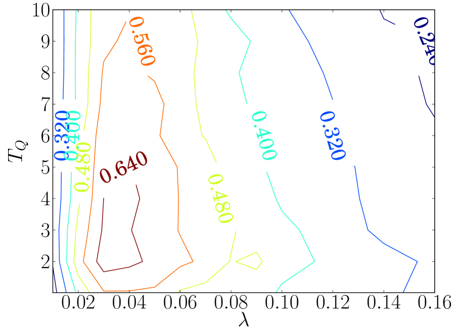
(a)

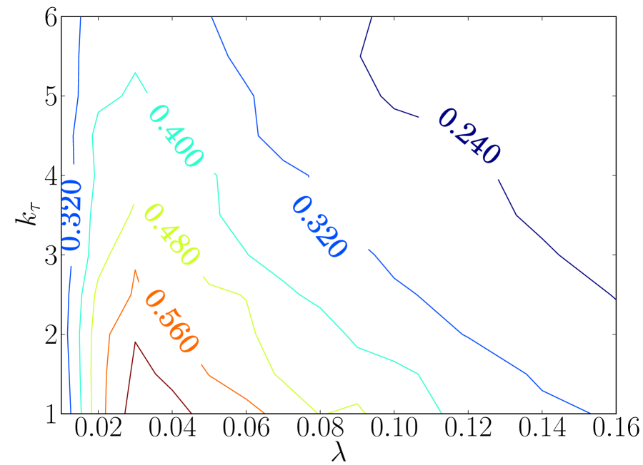
(b)

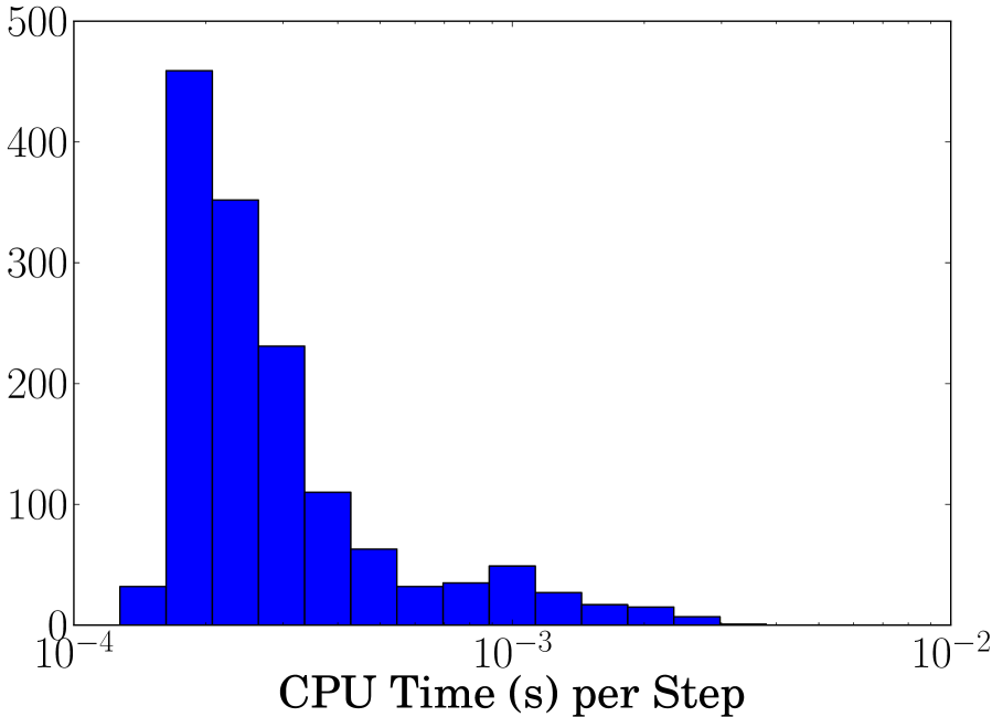
(c)

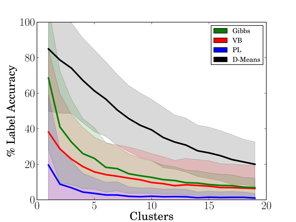
(d)

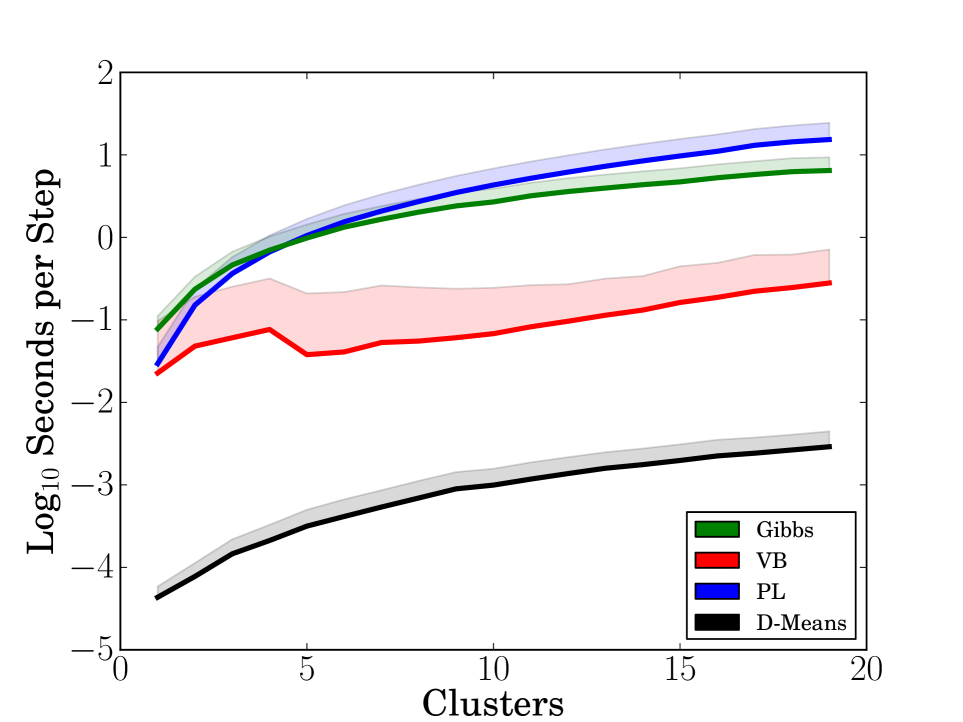
(e)

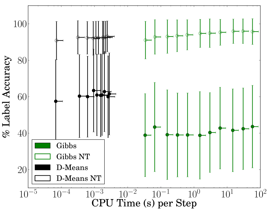
(f)

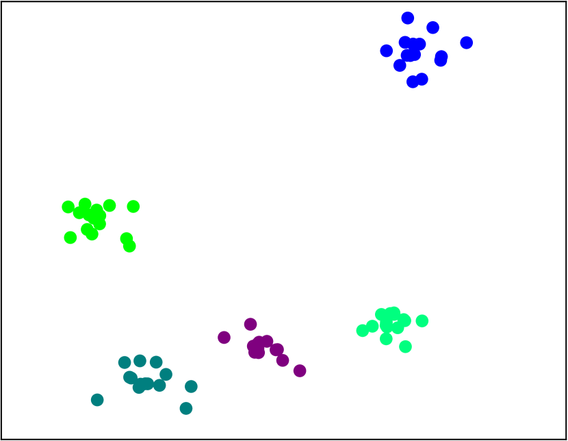
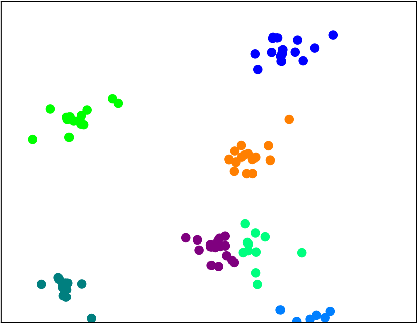
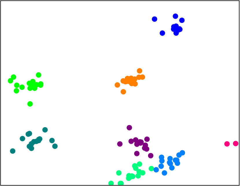
(g)

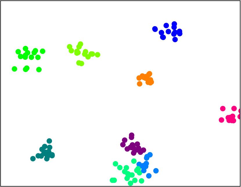
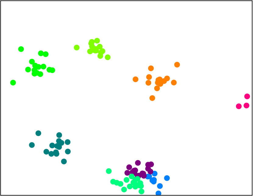
Figure 1: (1(a) - 1(c)): Accuracy contours and CPU time histogram for D-Means. (1(d) - 1(e)): Comparison with Gibbs sampling, variational inference, and particle learning. Shaded region indicates $1\sigma$ interval; in (1(e)), only upper half is shown. (1(f)): Comparison of accuracy when enforcing (Gibbs, D-Means) and not enforcing (Gibbs NT, D-Means NT) correct cluster tracking. (1(g)): An example 5 sequential frames from clustering using D-Means; note the consistency of datapoint labelling (color) over time.

The first experiment was designed to provide an empirical backing to the theoretical developments in the foregoing sections. This was achieved through the use of synthetic mixture model data, with known cluster assignments for accuracy comparisons. In particular, moving Gaussian clusters on $[0,1]\times[0,1]$ were generated over a period of 100 time steps, with the number of clusters fixed. At each time step, each cluster had 15 data points sampled from a isotropic Gaussian distribution with a standard deviation of 0.05. Between time steps, the cluster centers moved randomly, with displacements sampled from the same distribution. At each time step, each cluster had a 0.05 probability of being destroyed, and upon destruction a new cluster was created with a random location in the domain. This experiment involved four algorithms: D-Means with 3 random assignment ordering restarts; Gibbs sampling on the full MCGMM with 5000 samples (Lin et al., 2010); variational inference to a tolerance of $10^{-16}$ (Blei and Jordan, 2006); and particle learning with 100 particles (Carvalho et al., 2010b).

First, the parameter space of each algorithm was searched for the best average cluster label accuracy over 50 trials when the number of clusters was fixed to 5. The results of this parameter sweep for D-Means are shown in Figures 1(a)–1(c). Figures 1(a) and 1(b) show how the average clustering accuracy varies with the parameters, after fixing either $k_{\tau}$ or $T_{Q}$ to their values at the maximum accuracy setting. D-Means had a similar robustness with respect to variations in its parameters as the other algorithms. The histogram in Figure 1(c) demonstrates that the clustering speed is robust to the setting of parameters. The speed of Dynamic Means, coupled with the smoothness of its performance with respect to its parameters, makes it well suited for automatic tuning (Snoek et al., 2012).

Using the best parameter setting for D-Means ($\lambda=0.04$, $T_{Q}=6.8$, and $k_{\tau}=1.01$) and the true generative model parameters for Gibbs/PL/VB, the data were clustered in 50 trials with a varying number of clusters present in the data. In Figures 1(d) and 1(e), the labeling accuracy and clustering time for the algorithms is shown versus the true number of clusters in the domain. Since the domain is bounded, increasing the true number of clusters makes the labeling of individual data more ambiguous, yielding lower accuracy for all algorithms. These results illustrate that D-Means outperforms standard inference algorithms in both label accuracy and computational cost for cluster tracking problems.

Note that the sampling algorithms were handicapped to generate Figure 1(d); the best posterior sample in terms of labeling accuracy was selected at each time step, which required knowledge of the true labeling. Further, the accuracy computation involved solving a maximum matching problem between the learned and true data labels at each timestep, and then removing all correspondences inconsistent with matchings from previous timesteps, thus enforcing consistent cluster tracking over time. If inconsistent correspondences aren’t removed (i.e. label accuracy computations consider each time step independently), the other algorithms provide accuracies more comparable to those of D-Means. This effect is demonstrated in Figure 1(f), which shows the time/accuracy tradeoff for D-means (varying the number of restarts) and MCGMM (varying the number of samples) when label consistency is enforced, and when it is not enforced.

8.2 Synthetic Moving Rings

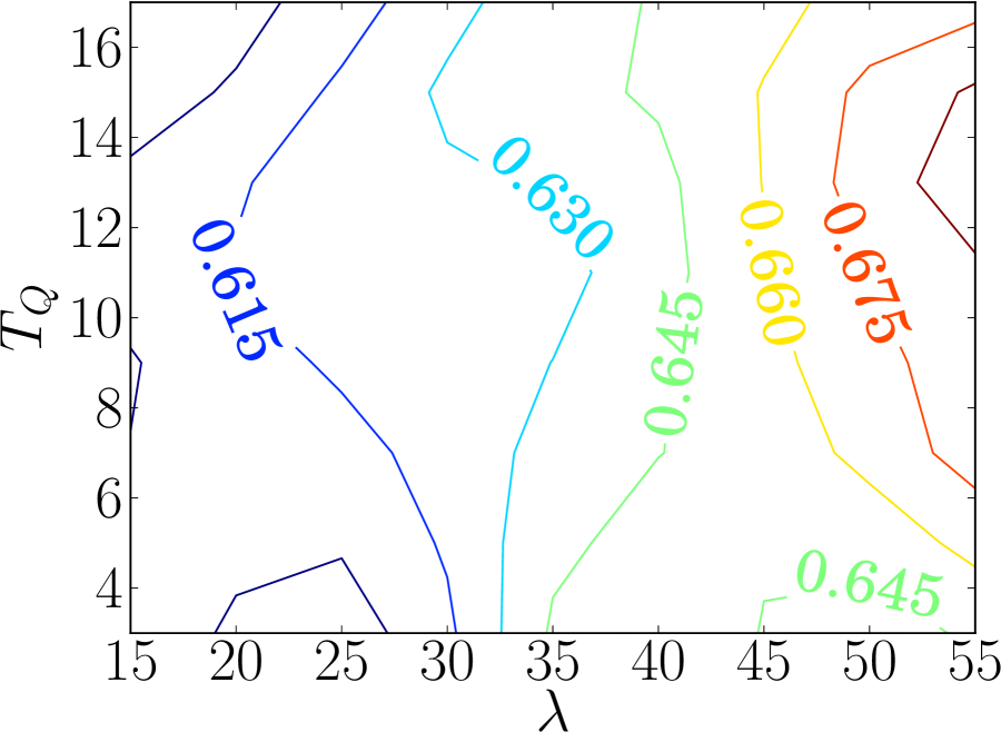
(a)

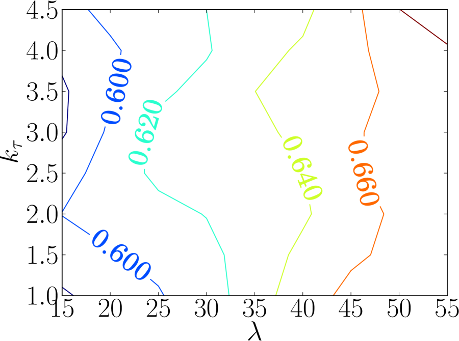
(b)

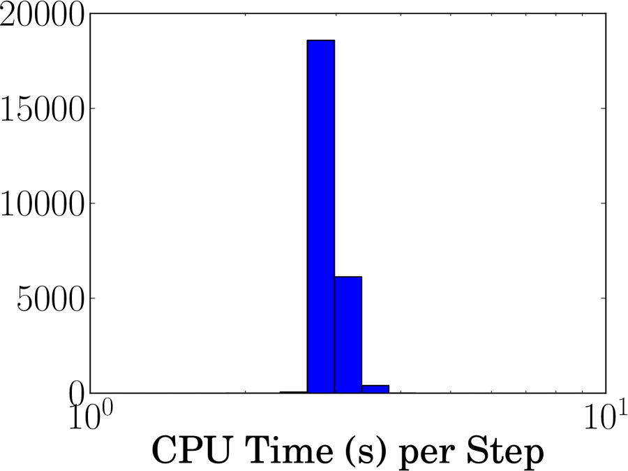
(c)

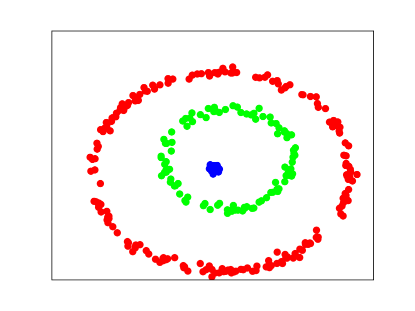
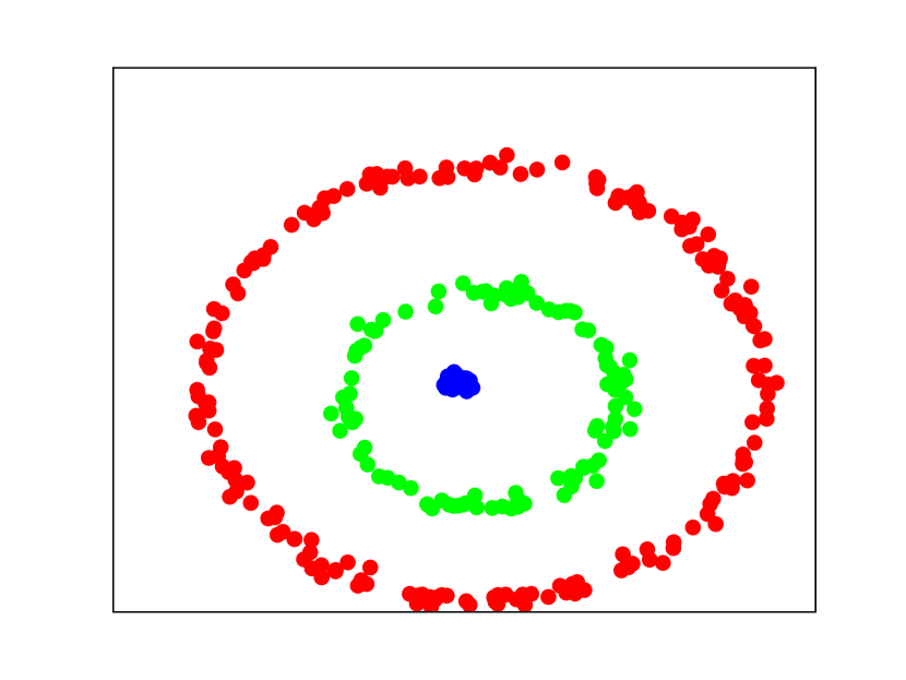
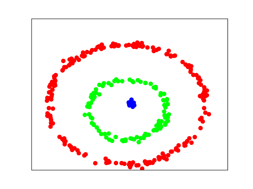
(d)

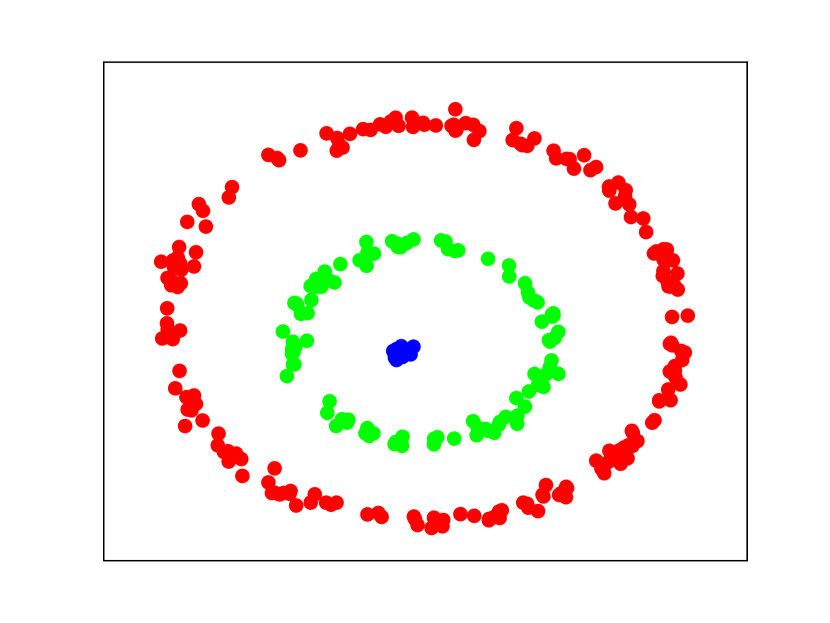
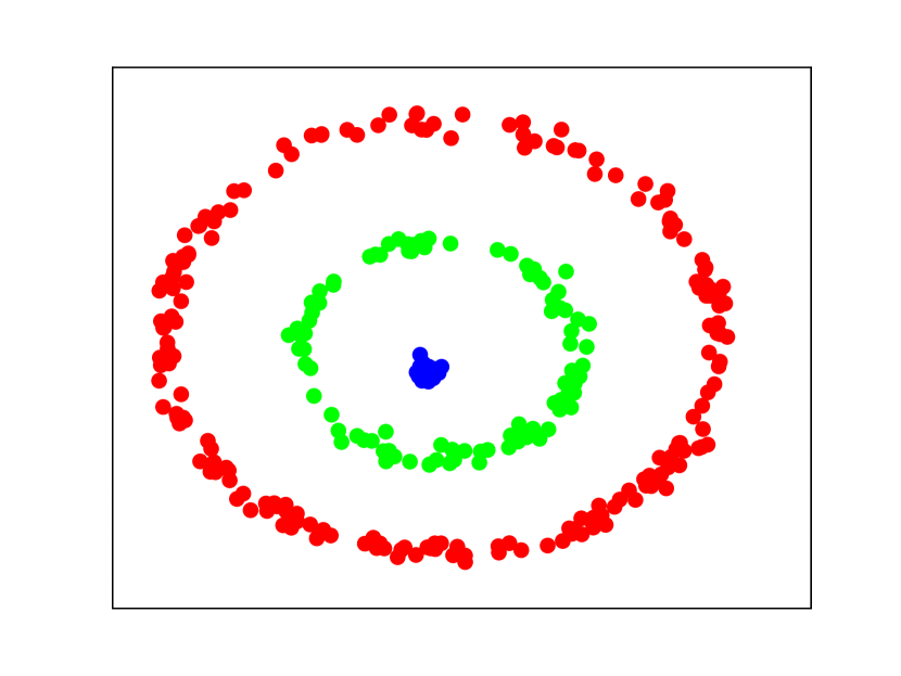
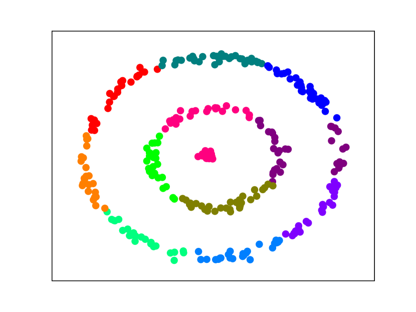
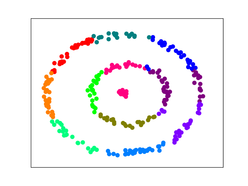
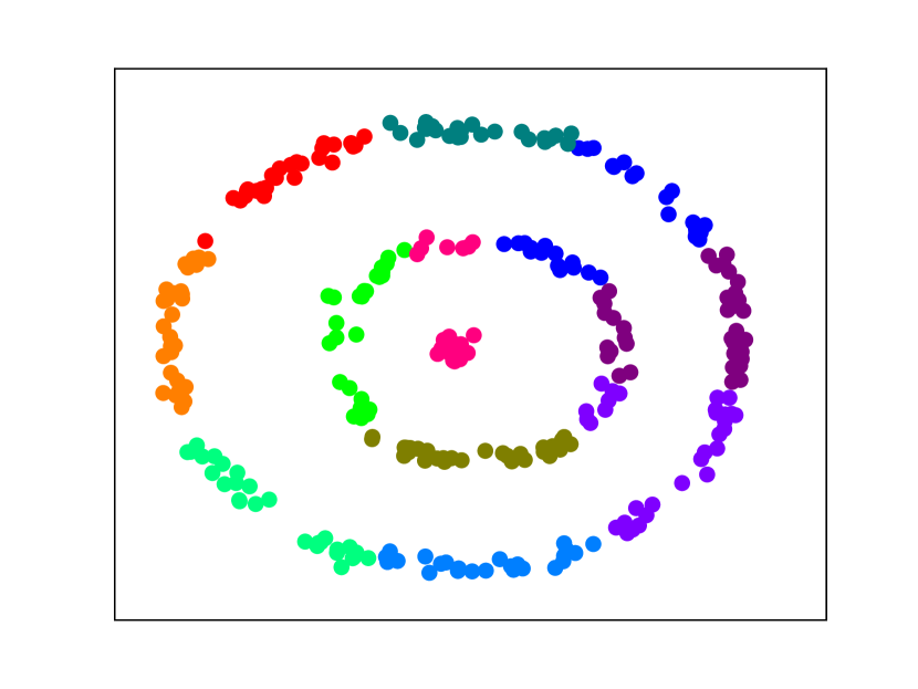
(e)

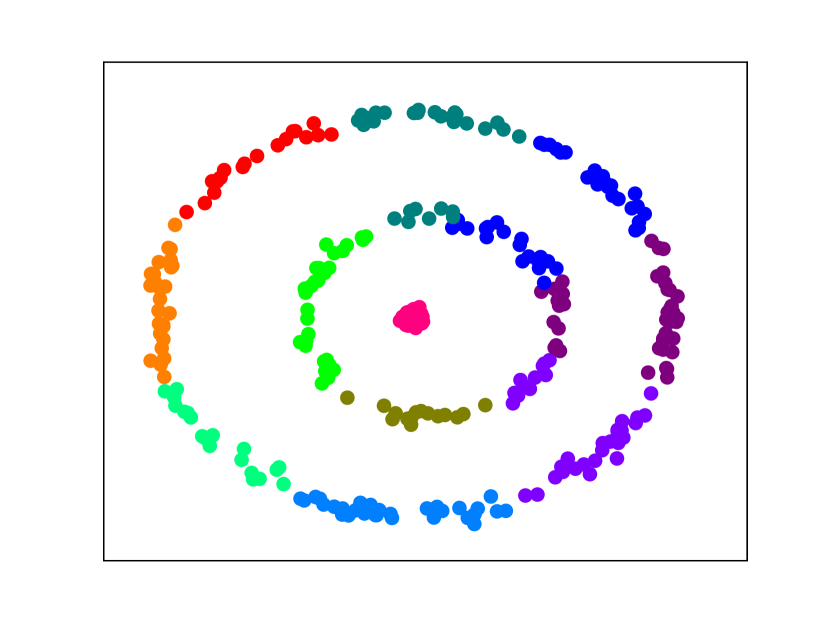
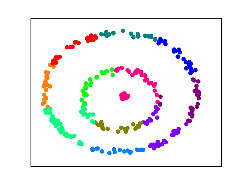
Figure 2: (2(a) - 2(c)): Accuracy contours and CPU time histogram for SD-Means on the synthetic ring data. (2(d) - 2(e)) An example 5 sequential frames from clustering using SD-Means (2(d)) and D-Means (2(e)).

To illustrate the strengths of SD-Means with respect to D-Means, a second synthetic dataset of moving concentric rings was clustered in the same $[0,1]\times[0,1]$ domain. At each

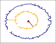
Figure 3: MST kernel to the center point.

time step, 400 datapoints were generated uniformly randomly on 3 rings of radius 0.4, 0.2, and 0.0 respectively, with added isotropic Gaussian noise of standard deviation 0.03. Between time steps, the three rings moved randomly, with displacements sampled from an isotropic Gaussian of standard deviation 0.05. The kernel function for SD-Means between two points $y_{1},y_{2}$ was $\exp\left(-\frac{d^{2}}{2\omega^{2}}\right)$, where $\omega=0.07$ was a constant, and $d$ was the sum of distances greater than $\omega$ along the path connecting $y_{1}$ and $y_{2}$ through the minimum Euclidean spanning tree of the dataset at each timestep. This kernel was used to capture long-range similarity between points on the same ring. An example of the minimum spanning tree and kernel function evaluation is shown in Figure 3. Finally, a similar parameter sweep to the previous experiment was used to find the best parameter settings for SD-Means ($\lambda=55$, $T_{Q}=13$, $k_{\tau}=4.5$) and D-Means ($\lambda=0.1$, $T_{Q}=15$, $k_{\tau}=1.1$).

Figure 2 shows the results from this experiment averaged over 50 trials. SD-Means exhibits a similar robustness to its parameter settings as D-Means on the moving Gaussian data, and is generally able to correctly cluster the moving rings. In contrast, D-Means is unable to capture the rings, due to their nonlinear separability, and introduces many erroneous clusters. Further, there is a significant computational cost to pay for the

Table 1: Mean computational time & accuracy on synthetic ring data over 50 trials.

Alg.	% Acc.	Time (s)
SD-Means	$75.1$	$2.9$
D-Means	$18.7$	$8.4\times 10^{-4}$

flexibility of SD-Means, as expected. Table 1 corroborates these observations with numerical data. Thus, in practice, D-Means should be the preferred algorithm unless the cluster structure of the data is not linearly separable, in which case the extra flexibility of SD-Means is required.

8.3 Synthetic Gaussian Processes

Clustering Gaussian processes (GPs) is problematic for many inference algorithms for a number of reasons. Sampling algorithms that update cluster parameters (such as DP-GP Gibbs sampling (Joseph et al., 2011)) require the inversion of kernel matrices for each sample, which is computationally intractable for large datasets. Many other algorithms, such as D-Means, require discretization of the GP mean function in order to compute distances, which incurs an exponential growth in computational complexity with the input dimension of the GP, increased susceptibility to local optima, and incapability to capture uncertainty in the areas of the GP with few measurements. SD-Means, on the other hand, can capture the GP uncertainty through the kernel function, and since cluster parameters are not instantiated while clustering each batch of data it does not incur the cost of repeated GP regression.

This experiment involved clustering noisy sets of observations from an unknown number $K$ of latent functions $f_{k}(\cdot)$. The uncertainty in the functions $f_{k}(\cdot)$ was captured by modelling them as GPs. The data were generated from $K=4$ functions: $f_{1}(x)=x$, $f_{2}(x)=-x$, $f_{3}(x)=\sin(x)$, and $f_{4}(x)=\cos(x)$. For each data point to be clustered, a random label $k\in\{1,2,3,4\}$ was sampled uniformly, along with a random interval in $[0,1]$. Then 30 $x,y$ pairs were generated within the interval with uniformly random $x$ and $y=f_{k}(x)+\epsilon$, $\epsilon\sim\mathcal{N}(0,0.2^{2})$. These $x,y$ pairs were used to train a Gaussian process, which formed a single datapoint in the clustering procedure. Measurements were made in a random interval to ensure that large areas of the domain of each GP had a high uncertainty, in order to demonstrate the robustness of SD-Means to GP uncertainty. Example GPs generated from this procedure, with $1\sigma$ measurement confidence bounds, are shown in Figure LABEL:fig:datagps. D-Means and SD-Means were used to cluster a dataset of 1000 such GPs, broken into batches of 100 GPs. For D-Means, the GP mean function was discretized on $[0,1]$ with a grid spacing of $0.02$, and the discretized mean functions were clustered. For SD-Means, the kernel function between two GPs $i$ and $j$ was the probability that their respective kernel points were generated from the same latent GP (with a prior probability of 0.5),

$$\kappa\!\left((X_{i},Y_{i}),(X_{j},Y_{j})\right) =\frac{\mathrm{GP}(Y_{i},Y_{j}|X_{i},X_{j})}{\mathrm{GP}(Y_{i},Y_{j}|X_{i},X_{j})+\mathrm{GP}(Y_{i}|X_{i})\mathrm{GP}(Y_{j}|X_{j})}$$ (52)

where $X_{i},Y_{i}$ are the domain and range of the kernel points for GP $i$, and $\mathrm{GP}\left(\cdot|\cdot\right)$ is the Gaussian process marginal likelihood function.

The results from this exercise are shown in Figures LABEL:fig:dmgps - LABEL:fig:gpaccnclus. Figures LABEL:fig:dmgps and LABEL:fig:sdmgps demonstrate that SD-Means tends to discover the 4 latent functions used to generate the data, while D-Means often introduces erroneous clusters. Figure LABEL:fig:gpaccnclus corroborates the qualitative results with a quantitative comparison over 300 trials, demonstrating that while D-Means is roughly 2 orders of magnitude faster, SD-Means generally outperforms D-Means in label accuracy and the selection of the number of clusters. This is primarily due to the fact that D-Means clusters data using only the GP means; as the GP mean function can be a poor characterization of the latent function (shown in Figure LABEL:fig:datagps), D-Means can perform poorly. SD-Means, on the other hand, uses a kernel function that accounts for regions of high uncertainty in the GPs, and thus is generally more robust to such uncertainty.

8.4 Aircraft ADSB Trajectories

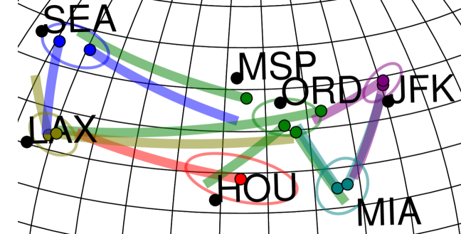
(a)

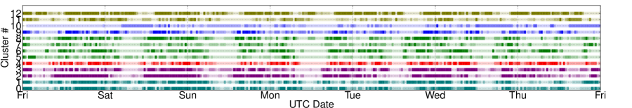
(b)

Figure 4: Results of the GP aircraft trajectory clustering. (4(a)): A map (labeled with major US city airports) showing the overall aircraft flows for 12 trajectories, with colors and 1$\sigma$ confidence ellipses corresponding to takeoff region (multiple clusters per takeoff region), colored dots indicating mean takeoff position for each cluster, and lines indicating the mean trajectory for each cluster. (4(b)): A track of plane counts for the 12 clusters during the week, with color intensity proportional to the number of takeoffs at each time.

In this experiment, the D-Means algorithm was used to discover the typical spatial and temporal patterns in the motions of commercial aircraft. The experiment was designed to demonstrate the capability of D-Means to find spatial and temporal patterns in a streaming source of real world data over a long duration.

The data was collected and processed using the following procedure. Automatic dependent surveillance-broadcast (ADS-B) data, including plane identification, timestamp, latitude, longitude, heading and speed, was collected from all transmitting planes across the United States during the week from 2013-3-22 1:30:0 to 2013-3-28 12:0:0 UTC. Then, individual ADS-B messages were connected together based on their plane identification and timestamp to form trajectories, and erroneous trajectories were filtered based on reasonable spatial/temporal bounds, yielding 17,895 unique trajectories. Then, each trajectory was smoothed by training a Gaussian process, where the latitude and longitude of points along the trajectory were the inputs, and the North and East components of plane velocity at those points were the outputs. Next, the mean latitudinal and longitudinal velocities from the Gaussian process were queried for each point on a regular lattice across the United States (10 latitudes and 20 longitudes), and used to create a 400-dimensional feature vector for each trajectory. Of the resulting 17,895 feature vectors, 600 were hand-labeled, including a confidence weight between 0 and 1. The feature vectors were clustered in half-hour batch windows using D-Means (3 restarts), MCGMM Gibbs sampling (50 samples), and the DP-Means algorithm (Kulis and Jordan, 2012) (3 restarts, run on the entire dataset in a single batch).

Table 2: Mean computational time & accuracy on hand-labeled aircraft trajectory data

Alg.	% Acc.	Time (s)
D-Means	$55.9$	$2.7\times 10^{2}$
DP-Means	$55.6$	$3.1\times 10^{3}$
Gibbs	$36.9$	$1.4\times 10^{4}$

The results of this exercise are provided in Figure 4 and Table 2. Figure 4 shows the spatial and temporal properties of the 12 most popular clusters discovered by D-Means, demonstrating that the algorithm successfully identified major flows of commercial aircraft across the United States. Table 2 corroborates these qualitative results with a quantitative comparison of the computation time and accuracy for the three algorithms tested over 20 trials. The confidence-weighted accuracy was computed by taking the ratio between the sum of the weights for correctly labeled points and the sum of all weights. The MCGMM Gibbs sampling algorithm was handicapped as described in the synthetic experiment section. Of the three algorithms, D-Means provided the highest labeling accuracy, while requiring the least computational time by over an order of magnitude.

8.5 Video Color Quantization

Video is an ubiquitous form of naturally batch-sequential data – the sequence of image frames in a video can be considered a sequence of batches of data. In this experiment, the colors of a video were quantized via clustering. Quantization, in which each image pixel is assigned to one of a small palette of colors, can be used both as a component of image compression algorithms and as a visual effect. To find an appropriate palette for a given image, a clustering algorithm may be applied to the set of colors from all pixels in the image, and the cluster centers are extracted to form the palette.

Video frame sequences typically undergo smooth evolution interspersed with discontinuous jumps; D-Means is well-suited to clustering such data, with motion processes to capture the smooth evolution, and birth/death processes to capture the discontinuities. As a color quantization algorithm, D-Means yields a smoothly varying palette of colors, rather than a palette for each frame individually. The parameters used were $\lambda=800$, $T_{Q}=15$, $K_{\tau}=1.1$. For comparison, two other algorithms were run on each frame of the same video individually: DP-Means with $\lambda=800$ and K-Means with $K=20$. The video selected for the experiment was Sintel, consisting of 17,904 frames at $1280\times 544$ resolution.

The results of the experiment are shown in Figure 5 with example quantized frames shown in Figure 5(a). The major advantage of using D-Means over DP-Means or K-Means is that color flicker in the quantization is significantly reduced, as evidenced by Figures 5(b)-5(d). This is due to the cluster motion modeling capability of D-Means – by enforcing that cluster centers vary smoothly over time, the quantization in sequential frames is forced to be similar, yielding a temporally smooth quantization. In contrast, the cluster centers for K-Means or DP-Means can differ significantly from frame to frame, causing noticeable flicker to occur, thus detracting from the quality of the quantization.

(a)

(b)

(c)

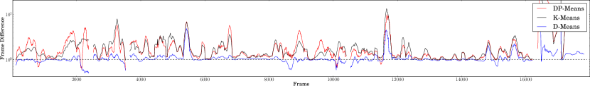
(d)

Figure 5: Video color quantization results. (5(a)): Four frames from the original video (top row) and quantized video (bottom row) with D-Means. (5(b)): The number of clusters over the whole video (top) and a zoomed window on frames 3550-4350 (bottom). Note the smoothness of the number of clusters over time using D-Means with respect to DP-Means. (5(c)): A sequence of 4 frames from the original video (top row), quantized video with D-Means (middle row), and quantized video with DP-Means (bottom row). Note the flicker in the quantization, particularly in the upper region of the frames, when using DP-Means in contrast to using D-Means. (5(d)): The difference between each frame and the previous frame for quantized video, normalized by the same quantity for the original video. D-Means tracks the original video (dashed horizontal black line) more closely than both K-Means and DP-Means. Missing values are when the original video had no frame difference (normalization by 0).

8.6 Human Segmentation in Point Clouds

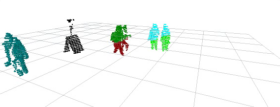
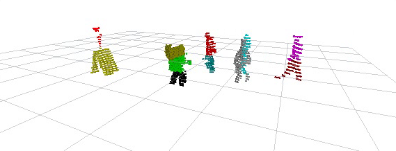
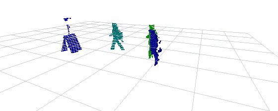
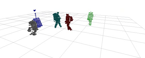
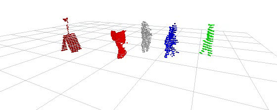
Figure 6: Comparison of D-Means (top row) and SD-Means (bottom row) on four frames of the point cloud dataset. Color indicates cluster assignment. Note that D-Means is forced to either oversegment humans or erroneously group them together, while SD-Means correctly clusters them.

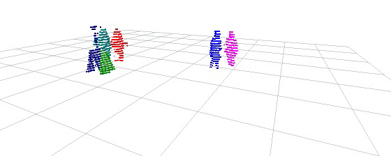
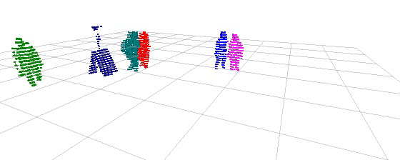
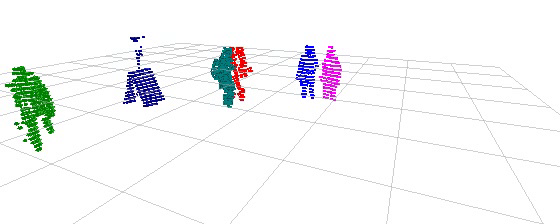
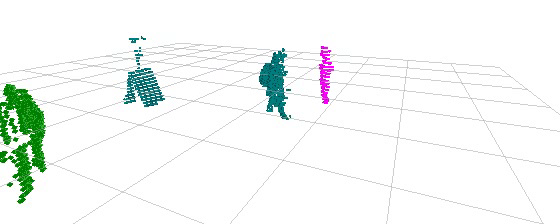
Figure 7: Cluster assignments from SD-Means for a sequence of four frames from the point cloud dataset. Color indicates cluster assignment. Note the temporal consistency of the clustering, and the flexibility to temporarily remove clusters when humans are occluded.

Batch-sequential data is also prevalent in the field of mobile robotics, where point cloud sequences provided by LiDAR and RGB-D sensors are commonly used for perception. In this experiment, D-Means and SD-Means were used to cluster 120 seconds of LiDAR data, at 30 frames per second, of people walking in a foyer. The experiment was designed to demonstrate the capability of SD-Means to simultaneously cluster nonspherical shapes and track them over time. For comparison of the two algorithms, the point clouds were hand-labeled with each human as a single cluster.

Table 3: Computational time & accuracy on point cloud dataset.

Alg.	% Acc.	Time (s)
SD-Means	$86.8$	$816.7$
D-Means	$53.6$	$38.1$

The results are shown in Figures 6 - 7 and Table 3. Figure 6 shows that D-Means cannot capture the complex cluster structure present in the dataset – due to the spherical cluster assumption made by the algorithm, changing the parameter $\lambda$ causes D-Means to either over- or undersegment the humans. In contrast, SD-Means captures the structure and segments the humans accordingly. Figure 7 demonstrates the ability of SD-Means to correctly capture temporal evolution of the clusters in the dataset, due to its derivation from the MCGMM. Table 3 corroborates these findings numerically, by showing that SD-Means provides much higher point labeling accuracy on the dataset than D-Means (using the same label accuracy computation as outlined in previous experiments).

9 Conclusions

This work presented the first small-variance analysis for Bayesian nonparametric models that capture batch-sequential data containing temporally evolving clusters. While previous small-variance analyses have exclusively focused on models trained on a single, static batch of data, this work provides evidence that the small-variance methodology yields useful results for evolving models. In particular, the present work developed two new clustering algorithms: The first, D-Means, was derived from a small-variance asymptotic analysis of the low-variance MAP filtering problem for the MCGMM; and the second, SD-Means, was derived from a kernelization and spectral relaxation of the D-Means clustering problem. Empirical results from both synthetic and real data experiments demonstrated the performance of the algorithms compared with contemporary probabilistic and hard clustering algorithms.

10 Acknowledgements

We would like to acknowledge support for this project from the National Science Foundation (NSF CAREER Award 1559558) and the Office of Naval Research (ONR MURI grant N000141110688). We would also like to thank Miao Liu for discussions and help with algorithmic implementations.

Appendix A The Equivalence Between Dynamic Means and Small-Variance MCGMM Gibbs Sampling

A.1 Setting Labels Given Parameters

In the label sampling step, a datapoint $y_{it}$ can either create a new cluster, join a current cluster, or revive an old, transitioned cluster. Thus, the label assignment probabilities are

$$p(z_{it}=k|\dots)\propto$$ (53)

$$\left\{\begin{array}[]{c c}\alpha(2\pi(\sigma+\rho))^{-d/2}\exp{\left({-\frac{||y_{it}-\phi||^{2}}{2(\sigma+\rho)}}\right)}&k=K_{t}+1\\ (c_{kt}+n_{kt})(2\pi\sigma)^{-d/2}\exp{\left({-\frac{||y_{it}-\theta_{kt}||^{2}}{2\sigma}}\right)}&n_{kt}>0\\ q^{{\Delta t}_{kt}}c_{kt}(2\pi(\sigma+\xi{{\Delta t}_{kt}}+\rho_{kt}))^{-d/2}\exp{\left({-\frac{||y_{it}-\phi_{kt}||^{2}}{2(\sigma+\xi{{\Delta t}_{kt}}+\rho_{kt})}}\right)}&n_{kt}=0,\end{array}\right.$$ (57)

and the parameter scaling in (17) yields the following deterministic assignments as $\sigma\rightarrow 0$:

$$z_{it}=\operatorname*{argmin}_{k}\left\{\begin{array}[]{l l}||y_{it}-\theta_{kt}||^{2}&\text{if $\theta_{k}$ instantiated}\\ Q{{\Delta t}_{kt}}+\frac{\gamma_{kt}}{\gamma_{kt}+1}||y_{it}-\phi_{kt}||^{2}&\text{if $\theta_{k}$ old, uninstantiated}\\ \lambda&\text{if $\theta_{k}$ new}\end{array}\right..$$ (61)

which is exactly the label assignment step from Section 4.

A.2 Setting Parameters Given Labels

In the parameter sampling step, the parameters are sampled using the distribution

$$p(\theta_{kt}|\{y_{it}:z_{it}=k\})\propto p(\{y_{it}:z_{it}=k\}|\theta_{kt})p(\theta_{kt}).$$ (62)

Suppose there are ${{\Delta t}_{kt}}$ time steps where cluster $k$ was not observed, but there are now $n_{kt}$ data points assigned to it in the current time step. Thus,

$$p(\theta_{kt})=\int_{\theta}T(\theta_{kt}|\theta)p(\theta)\,\mathrm{d}\theta,\,\,\theta\sim\mathcal{N}(\phi_{kt},\rho_{kt}).$$ (63)

where $\phi_{kt}$ and $\rho_{kt}$ capture the uncertainty in cluster $k$ ${{\Delta t}_{kt}}$ timesteps ago when it was last observed. Again using conjugacy of normal likelihoods and priors,

$$\begin{aligned} \theta_{kt}|\{y_{it}:z_{it}=k\}&\sim\mathcal{N}\left(\theta_{\text{post}},\sigma_{\text{post}}\right)\\ \theta_{\text{post}}=\sigma_{\text{post}}\left(\frac{\phi_{kt}}{\xi{{\Delta t}_{kt}}+\rho_{kt}}+\frac{\sum_{i:z_{it}=k}y_{it}}{\sigma}\right)&,\,\sigma_{\text{post}}=\left(\frac{1}{\xi{{\Delta t}_{kt}}+\rho_{kt}}+\frac{n_{kt}}{\sigma}\right)^{-1}.\end{aligned}$$ (64)

Similarly to the label assignment step, let $\xi=\tau\sigma$. Then as long as $\rho_{kt}=\sigma/w_{kt}$, $w_{kt}>0$ (which holds if equation (64) is used to recursively keep track of the parameter posterior), taking the asymptotic limit of this as $\sigma\rightarrow 0$ yields

$$\theta_{kt} =\frac{\phi_{kt}(w_{kt}^{-1}+{{\Delta t}_{kt}}\tau)^{-1}+\sum_{i\in\mathcal{I}_{kt}}y_{it}}{(w_{kt}^{-1}+{{\Delta t}_{kt}}\tau)^{-1}+n_{kt}}=\frac{\gamma_{kt}\phi_{kt}+\sum_{i\in\mathcal{I}_{kt}}y_{it}}{\gamma_{kt}+n_{kt}}$$ (65)

Appendix B Proof of Stability of the Old Cluster Center Approximation

• The error of the approximation $\epsilon_{t+1}$ at time $t+1$ can be bounded given an error bound for the optimization $\epsilon$ and the error bound at time $t$:

  $$\begin{aligned} \epsilon_{t+1}&=\|\phi_{k(t+1)}-\phi^{\star}_{k(t+1)}\|_{2}=\|\phi_{k(t+1)}-\bar{\phi}_{k(t+1)}+\bar{\phi}_{k(t+1)}-\phi^{\star}_{k(t+1)}\|_{2}.\end{aligned}$$ (66)

  Using the fact that $\bar{\phi}_{k(t+1)}$ is the dense approximation of $\phi^{\star}_{k(t+1)}$, i.e. including all data assigned to cluster $k$ at timestep $t$, this is equal to

  $$\begin{aligned} &=\|\phi_{k(t+1)}-\bar{\phi}_{k(t+1)}+\left(\frac{\gamma_{kt}(\phi_{kt}-\phi^{\star}_{kt})}{\gamma_{kt}+n_{kt}}\right)\|_{2}\\ &\leq\|\phi_{k(t+1)}-\bar{\phi}_{k(t+1)}\|_{2}+\frac{\gamma_{kt}}{\gamma_{kt}+n_{kt}}\|\phi_{kt}-\phi^{\star}_{kt}\|_{2}\\ &\leq\epsilon+\frac{\gamma_{kt}}{\gamma_{kt}+n_{kt}}\epsilon_{t}.\end{aligned}$$ (67)

  Now using the facts that $\gamma_{kt}=\left(w_{kt}^{-1}+\tau{{\Delta t}_{kt}}\right)^{-1}$, $w_{kt}>0$, ${{\Delta t}_{kt}}\geq 1$, and $n_{kt}\geq 1$,

  $$\epsilon_{t+1} \leq\epsilon+\frac{1}{1+\tau}\epsilon_{t}.$$ (68)

  Expanding the recursion and using the geometric series formula,

  $$\begin{aligned} \epsilon_{t}&\leq\sum_{i=0}^{t-1}\left(\frac{1}{1+\tau}\right)^{i}\epsilon=\epsilon\frac{1-\left(\frac{1}{1+\tau}\right)^{t}}{1-\left(\frac{1}{1+\tau}\right)}\leq\epsilon\left(1+\frac{1}{\tau}\right).\end{aligned}$$ (69)

  ∎

Appendix C Proof of Integrality/Optimality of the Cluster Matching

Lemma 2 (Ghouila-Houri 1962).

Consider a matrix $A$ with $n$ rows of the form $r\in\mathbb{R}^{1\times n}$. $A$ is totally unimodular iff for every subset $R$ of the rows, there is a partition of $R$, $R_{+}\cup R_{-}=R$, $R_{+}\cap R_{-}=\emptyset$, such that

$$\left[\sum_{r\in R_{+}}r\right]-\left[\sum_{r\in R_{-}}r\right]\in\{0,1,-1\}^{1\times n}.$$ (70)

Proof.

This result is proven in (Schrijver, 2003). ∎

• The constraints of the linear program (51) are as follows:

  $$\begin{aligned} &\sum_{k=1}^{K_{t-1}}c_{lk}\leq 1,\,\,1\leq j\leq\left|\mathcal{A}_{t}\right|\\ &\sum_{l=1}^{\left|\mathcal{A}_{t}\right|}c_{lk}\leq 1,\,\,1\leq k\leq K_{t-1}\\ &c\geq 0,\,\,c\in\mathbb{R}^{\left|\mathcal{A}_{t}\right|\times K_{t-1}}.\end{aligned}$$ (71)

  To show that this set of constraints has a totally unimodular matrix, we use Lemma 2. Given any subset $R$ of the constraints, let $R^{\prime}_{+}$ consist of the coefficient vectors from all constraints of the form $\sum_{l=1}^{\left|\mathcal{A}_{t}\right|}c_{lk}\leq 1$, and let $R^{\prime}_{-}$ consist of the coefficient vectors from all constraints of the form $\sum_{k=1}^{K_{t-1}}c_{lk}\leq 1$. Then since every variable $c_{lk}$ has a $1$ coefficient in exactly one constraint of the former type and a $1$ coefficient in exactly one constraint of the latter type,

  $$\left[\sum_{r\in R^{\prime}_{+}}r\right]-\left[\sum_{r\in R^{\prime}_{-}}r\right]\equiv\tilde{r}\in\{0,1,-1\}^{1\times N}.$$ (72)

  Then, let $R^{\prime\prime}_{+}$ consist of the rows in $R$ corresponding to the individual nonnegativity constraints $c_{lk}\geq 0$ in which $\tilde{r}$ has a $-1$ or $0$ entry in the column for $c_{lk}$, and let $R^{\prime\prime}_{-}$ be the remaining nonnegativity constraint rows. Finally, let $R_{+}=R^{\prime}_{+}\cup R^{\prime\prime}_{+}$, and let $R_{-}=R^{\prime}_{-}\cup R^{\prime\prime}_{-}$. With this setting of $R_{+}/R_{-}$, the condition in Lemma 2 holds, and therefore the constraint matrix is totally unimodular. ∎

• By adding slack variables $s_{l}=1-\sum_{k=1}^{K_{t-1}}c_{lk}$, the optimization (51) can be rewritten in the following form:

  $$\begin{aligned} c^{\star}=\operatorname*{argmin}_{c,s}\quad&\sum_{l=1}^{\left|\mathcal{A}_{t}\right|}\left(s_{l}m_{l}+\sum_{k=1}^{K_{t-1}}c_{lk}m_{lk}\right)\\ \mathrm{s.t.}\quad&\sum_{k=1}^{K_{t-1}}c_{lk}+s_{l}=1,\,\,1\leq l\leq\left|\mathcal{A}_{t}\right|\\ &\sum_{k=1}^{\left|\mathcal{A}_{t}\right|}c_{lk}\leq 1,\,\,1\leq k\leq K_{t-1}\\ &c,s\geq 0,\quad c\in\mathbb{R}^{\left|\mathcal{A}_{t}\right|\times K_{t-1}},\quad s\in\mathbb{R}^{\left|\mathcal{A}_{t}\right|}\end{aligned}$$ (73)

  where $m_{l}$ is the cost of making temporary cluster $l$ a new cluster, and $m_{lk}$ is the cost of reinstantiating old cluster $k$ with temporary cluster $l$,

  $$\begin{aligned} m_{l}&=\lambda-\frac{1}{n_{l}}\sum_{i,j\in\mathcal{I}_{r}}\kappa^{YY}_{ij}\\ m_{lk}&=Q{{\Delta t}_{kt}}+\frac{\gamma_{kt}n_{l}\kappa^{\Phi\Phi}_{kk}}{\gamma_{kt}+n_{l}}-\!\sum_{i\in\mathcal{I}_{l}}\!\frac{2\gamma_{kt}\kappa^{Y\Phi}_{ik}+\sum_{j\in\mathcal{I}_{l}}\kappa^{YY}_{ij}}{\gamma_{kt}+n_{l}}.\end{aligned}$$ (74)

  However, by Lemma 1, the optimization (51) has a totally unimodular constraint matrix, and as such it produces an integer solution. Thus, the constraints $c,s\geq 0,\,c\in\mathbb{R}^{\left|\mathcal{A}_{t}\right|\times K_{t-1}},\,s\in\mathbb{R}^{\left|\mathcal{A}_{t}\right|}$ in (73) can be replaced with integer constraints $c\in\{0,1\}^{\left|\mathcal{A}_{t}\right|\times K_{t-1}},\,s\in\{0,1\}^{\left|\mathcal{A}_{t}\right|}$. By inspection of $m_{l}$ and $m_{lk}$, the resulting integer optimization directly minimizes (32) with respect to matchings between temporary clusters $l=1,\dots,\left|\mathcal{A}_{t}\right|$ and old/new clusters in the current timestep $t$. ∎

References

- Ahmed and Xing [2008] Amr Ahmed and Eric Xing. Dynamic non-parametric mixture models and the recurrent Chinese restaurant process with applications to evolutionary clustering. In International Conference on Data Mining, 2008.
- Akaike [1974] Hirotugu Akaike. A new look at the statistical model identification. IEEE Transactions on Automatic Control, 19(6):716–723, 1974.
- Banerjee et al. [2005] Arindam Banerjee, Srujana Merugu, Inderjit S. Dhillon, and Joydeep Ghosh. Clustering with Bregman divergences. Journal of Machine Learning Research, 6:1705–1749, 2005.
- Blei and Frazier [2011] David Blei and Peter Frazier. Distance dependent Chinese restaurant processes. Journal of Machine Learning Research, 12:2461–2488, 2011.
- Blei and Jordan [2006] David M. Blei and Michael I. Jordan. Variational inference for Dirichlet process mixtures. Bayesian Analysis, 1(1):121–144, 2006.
- Broderick et al. [2013] Tamara Broderick, Brian Kulis, and Michael Jordan. MAD-Bayes: MAP-based asymptotic derivations from Bayes. In Proceedings of the 30th International Conference on Machine Learning, 2013.
- Campbell et al. [2013] Trevor Campbell, Miao Liu, Brian Kulis, Jonathan P. How, and Lawrence Carin. Dynamic clustering via asymptotics of the dependent Dirichlet process. In Neural Information Processing Systems, 2013.
- Caron et al. [2007] Francois Caron, Manuel Davy, and Arnaud Doucet. Generalized Polya urn for time-varying Dirichlet process mixtures. In Uncertainty in Artificial Intelligence, 2007.
- Carvalho et al. [2010a] Carlos M. Carvalho, Michael S. Johannes, Hedibert F. Lopes, and Nicholas G. Polson. Particle learning and smoothing. Statistical Science, 25(1):88–106, 2010a.
- Carvalho et al. [2010b] Carlos M. Carvalho, Hedibert F. Lopes, Nicholas G. Polson, and Matt A. Taddy. Particle learning for general mixtures. Bayesian Analysis, 5(4):709–740, 2010b.
- Chakraborti et al. [2006] Deepayan Chakraborti, Ravi Kumar, and Andrew Tomkins. Evolutionary clustering. In Proceedings of the SIGKDD International Conference on Knowledge Discovery and Data Mining, 2006.
- Chen et al. [2013] Changyou Chen, Vinayak Rao, Wray Buntine, and Yee Whye Teh. Dependent normalized random measures. In International Conference on Machine Learning, 2013.
- Chi et al. [2007] Yun Chi, Xiaodan Song, Dengyong Zhou, Koji Hino, and Belle Tseng. Evolutionary spectral clustering by incorporating temporal smoothness. In Proceedings of the SIGKDD International Conference on Knowledge Discovery and Data Mining, 2007.
- Chi et al. [2009] Yun Chi, Xiaodan Song, Denyong Zhou, Koji Hino, and Belle Tseng. On evolutionary spectral clustering. ACM Transactions on Knowledge Discovery and Data Mining, 3(4:17), 2009.
- Dhillon et al. [2007] Inderjit Dhillon, Yuqiang Guan, and Brian Kulis. Weighted graph cuts without eigenvectors: A multilevel approach. IEEE Transactions on Pattern Analysis and Machine Intelligence, 29(11):1944–1957, 2007.
- Doshi-Velez and Ghahramani [2009] Finale Doshi-Velez and Zoubin Ghahramani. Accelerated sampling for the Indian buffet process. In Proceedings of the International Conference on Machine Learning, 2009.
- Endres et al. [2005] Felix Endres, Christian Plagemann, Cyrill Stachniss, and Wolfram Burgard. Unsupervised discovery of object classes from range data using latent Dirichlet allocation. In Robotics Science and Systems, 2005.
- Ferguson [1973] Thomas S. Ferguson. A Bayesian analysis of some nonparametric problems. The Annals of Statistics, 1(2):209–230, 1973.
- Hjort [1990] Nils Lid Hjort. Nonparametric Bayes estimators based on beta processes in models for life history data. The Annals of Statistics, 18:1259–1294, 1990.
- Hoffman et al. [2013] Matt Hoffman, David Blei, Chong Wang, and John Paisley. Stochastic variational inference. Journal of Machine Learning Research, 14:1303–1347, 2013.
- Hofmann et al. [2008] Thomas Hofmann, Bernhard Schölkopf, and Alexander Smola. Kernel methods in machine learning. The Annals of Statistics, 36(3):1171–1220, 2008.
- Hue et al. [2002] Carine Hue, Jean-Pierre Le Cadre, and Patrick Pérez. Tracking multiple objects with particle filtering. IEEE Transactions on Aerospace and Electronic Systems, 38(3):791–812, 2002.
- Ishioka [2000] Tsunenori Ishioka. Extended k-means with an efficient estimation of the number of clusters. In Proceedings of the 2nd International Conference on Intelligent Data Engineering and Automated Learning, pages 17–22, 2000.
- Jiang et al. [2012] Ke Jiang, Brian Kulis, and Michael Jordan. Small-variance asymptotics for exponential family Dirichlet process mixture models. In Advances in Neural Information Processing Systems, 2012.
- Joseph et al. [2011] Joshua Joseph, Finale Doshi-Velez, A. S. Huang, and N. Roy. A Bayesian nonparametric approach to modeling motion patterns. Autonomous Robots, 31(4):383–400, 2011.
- Kalnis et al. [2005] Panos Kalnis, Nikos Mamoulis, and Spiridon Bakiras. On discovering moving clusters in spatio-temporal data. In Proceedings of the 9th International Symposium on Spatial and Temporal Databases, pages 364–381. Springer, 2005.
- Kulis and Jordan [2012] Brian Kulis and Michael I. Jordan. Revisiting k-means: New algorithms via Bayesian nonparametrics. In Proceedings of the 29th International Conference on Machine Learning (ICML), Edinburgh, Scotland, 2012.
- Leskovec et al. [2005] Jure Leskovec, Jon Kleinberg, and Christos Faloutsos. Graphs over time: Densification laws, shrinking diameters and possible explanations. In Proceedings of the Eleventh ACM SIGKDD International Conference on Knowledge Discovery in Data Mining, pages 177–187. ACM, 2005.
- Lin et al. [2010] Dahua Lin, Eric Grimson, and John Fisher. Construction of dependent Dirichlet processes based on Poisson processes. In Neural Information Processing Systems, 2010.
- Lloyd [1982] Stuart P. Lloyd. Least squares quantization in PCM. IEEE Transactions on Information Theory, 28(2):129–137, 1982.
- Luber et al. [2004] Matthias Luber, Kai Arras, Christian Plagemann, and Wolfram Burgard. Classifying dynamic objects: An unsupervised learning approach. In Robotics Science and Systems, 2004.
- MacEachern [1999] Steven N. MacEachern. Dependent nonparametric processes. In Proceedings of the Bayesian Statistical Science Section. American Statistical Association, 1999.
- Neal [2000] Radford M. Neal. Markov chain sampling methods for Dirichlet process mixture models. Journal of Computational and Graphical Statistics, 9(2):249–265, 2000.
- Ning et al. [2010] Huazhong Ning, Wei Xu, Yun Chi, Yihong Gong, and Thomas Huang. Incremental spectral clustering by efficiently updating the eigen-system. Pattern Recognition, 43:113–127, 2010.
- Pelleg and Moore [2000] Dan Pelleg and Andrew Moore. X-means: Extending k-means with efficient estimation of the number of clusters. In Proceedings of the 17th International Conference on Machine Learning, 2000.
- Pitman [1995] Jim Pitman. Exchangeable and partially exchangeable random partitions. Probability Theory and Related Fields, 102:145–158, 1995.
- Roychowdhury et al. [2013] Anirban Roychowdhury, Ke Jiang, and Brian Kulis. Small-variance asymptotics for hidden Markov models. In Neural Information Processing Systems, 2013.
- Schrijver [2003] Alexander Schrijver. Combinatorial Optimization: Polyhedra and Efficiency. Springer, Berlin, 2003.
- Sethuraman [1994] Jayaram Sethuraman. A constructive definition of Dirichlet priors. Statistica Sinica, 4:639–650, 1994.
- Snoek et al. [2012] Jasper Snoek, Hugo Larochelle, and Ryan Adams. Practical Bayesian optimization of machine learning algorithms. In Neural Information Processing Systems, 2012.
- Spiliopoulou et al. [2006] Myra Spiliopoulou, Irene Ntoutsi, Yannis Theodoridis, and Rene Schult. MONIC - modeling and monitoring cluster transitions. In Proceedings of the 12th International Conference on Knowledge Discovering and Data Mining, pages 706–711, 2006.
- Sun et al. [2010] Yizhou Sun, Jie Tang, Jiawei Han, Manish Gupta, and Bo Zhao. Community evolution detection in dynamic heterogeneous information networks. In Proceedings of the 8th ACM Workshop on Mining and Learning with Graphs, pages 137–146, 2010.
- Tang et al. [2012] Lei Tang, Huan Liu, and Jianping Zhang. Identifying evolving groups in dynamic multimode networks. IEEE Transactions on Knowledge and Data Engineering, 24(1):72–85, 2012.
- Teh [2010] Yee Whye Teh. Dirichlet processes. In Encyclopedia of Machine Learning. Springer, New York, 2010.
- Thibaux and Jordan [2007] Romain Thibaux and Michael I. Jordan. Hierarchical beta processes and the Indian buffet process. In International Conference on Artificial Intelligence and Statistics, 2007.
- Tibshirani [1996] Robert Tibshirani. Regression shrinkage and selection via the Lasso. Journal of the Royal Statistical Society B, 58(1):267–288, 1996.
- Tibshirani et al. [2001] Robert Tibshirani, Guenther Walther, and Trevor Hastie. Estimating the number of clusters in a data set via the gap statistic. Journal of the Royal Statistical Society B, 63(2):411–423, 2001.
- Valgren et al. [2007] Christoffer Valgren, Tom Duckett, and Achim Lilienthal. Incremental spectral clustering and its application to topological mapping. In International Conference on Robotics and Automation, 2007.
- Vermaak et al. [2003] Jaco Vermaak, Arnaud Doucet, and Partick Pérez. Maintaining multi-modality through mixture tracking. In Proceedings of the 9th IEEE International Conference on Computer Vision, 2003.
- Wang et al. [2008] Zhikun Wang, Marc Deisenroth, Heni Ben Amor, David Vogt, Bernard Schölkopf, and Jan Peters. Probabilistic modeling of human movements for intention inference. In Robotics Science and Systems, 2008.
- Xu [2012] Kevin Xu. Computational Methods for Learning and Inference on Dynamic Networks. PhD thesis, The University of Michigan, 2012.
- Xu et al. [2012] Kevin Xu, Mark Kliger, and Alfred Hero III. Adaptive evolutionary clustering. Data Mining and Knowledge Discovery, pages 1–33, 2012.
- Xu et al. [2008a] Tianbing Xu, Zhongfei Zhang, Philip Yu, and Bo Long. Dirichlet process based evolutionary clustering. In Proceedings of the 8th IEEE International Conference on Data Mining, 2008a.
- Xu et al. [2008b] Tianbing Xu, Zhongfei Zhang, Philip Yu, and Bo Long. Evolutionary clustering by hierarchical Dirichlet process with hidden markov state. In Proceedings of the 8th IEEE International Conference on Data Mining, 2008b.
- Yu and Shi [2003] Stella Yu and Jianbo Shi. Multiclass spectral clustering. In Proceedings of the Ninth International Conference on Computer Vision, 2003.
- Zha et al. [2001] Hongyuan Zha, Xiaofeng He, Chris Ding, Horst Simon, and Ming Gu. Spectral relaxation for k-means clustering. In Advances in Neural Information Processing Systems, 2001.