Constraining the equation of state with identified particle spectra

Abstract

We show that in a central nucleus-nucleus collision, the variation of the mean transverse mass with the multiplicity is determined, up to a rescaling, by the variation of the energy over entropy ratio as a function of the entropy density, thus providing a direct link between experimental data and the equation of state. Each colliding energy thus probes the equation of state at an effective entropy density, whose approximate value is $19$ fm^-3 for Au+Au collisions at 200 GeV and $41$ fm^-3 for Pb+Pb collisions at 2.76 TeV, corresponding to temperatures of $227$ MeV and $279$ MeV if the equation of state is taken from lattice calculations. The relative change of the mean transverse mass as a function of the colliding energy gives a direct measure of the pressure over energy density ratio $P/\epsilon$, at the corresponding effective density. Using RHIC and LHC data, we obtain $P/\epsilon=0.21\pm 0.10$, in agreement with the lattice value $P/\epsilon=0.23$ in the corresponding temperature range. Measurements over a wide range of colliding energies using a single detector with good particle identification would help reducing the error.

I Introduction

One of the motivations for studying nucleus-nucleus collisions at high energies is to probe experimentally the equation of state of QCD matter Stoecker:1986ci . Ultrarelativistic collisions probe the phase diagram at vanishing chemical potential: at high temperatures, hadrons merge into a quark-gluon plasma. It was originally hoped that this change occurred through a first-order phase transition Yaffe:1982qf . However, it was progressively understood that it is a smooth, analytic crossover Brown:1990ev ; Aoki:2006we , and that a phase transition, if any deForcrand:2006pv , can only take place at high baryon density Fodor:2004nz ; Fukushima:2010bq . The equation of state of baryonless QCD matter is now known precisely from lattice simulations with physical quark masses Borsanyi:2010cj ; Bazavov:2014pvz . The goal of this paper is to understand the imprints of the equation of state on heavy-ion data, in particular transverse momentum spectra.

Relativistic hydrodynamics Gale:2013da plays a central role in our understanding of heavy-ion observables in the soft sector. Its simplest version is ideal hydrodynamics Kolb:2003dz , which describes most of the qualitative features seen in transverse momentum spectra, elliptic flow, and interferometry radii Huovinen:2006jp . This simple description can be refined by taking into account finite-size corrections due to viscosity Romatschke:2009im which are important for azimuthal anisotropies Heinz:2013th . The equation of state lies at the core of the hydrodynamic description, and the vast majority of modern hydrodynamic calculations Luzum:2008cw ; Schenke:2010rr ; Song:2010mg ; Bozek:2011ua ; Hirano:2010jg ; Petersen:2010cw ; Karpenko:2010te ; Akamatsu:2013wyk ; Holopainen:2010gz ; Pang:2012he ; Roy:2010qg , which give a satisfactory description of soft observables, use as an input an equation of state from lattice QCD calculations.

While the success of hydrodynamics suggests that equilibration takes place to some degree Gelis:2013rba ; Kurkela:2015qoa , most dynamical calculations predict that the system produced in the early stages of a heavy ion collision is far from chemical equilibrium, typically with overpopulation in gluon numbers Blaizot:2011xf and underpopulation in quark numbers Blaizot:2014jna ; Monnai:2014xya . The resulting effective equation of state might differ significantly from that calculated in lattice QCD, and it is important to understand what experimental data tell us about the equation of state, beyond a comparison between different lattice results Dudek:2014qoa ; Moreland:2015dvc . It has been recently shown that a simultaneous fit of several observables to hydrodynamic calculations constrains the equation of state to some extent Pratt:2015zsa . However, this recent study uses a systematic, Bayesian framework, and the nature of the relationships between model parameters and observables remains obscure. Further Bayesian studies have shown Sangaline:2015isa that interferometry radii and transverse momentum spectra are the observables which are most sensitive to the equation of state, but they are still unable to provide a simple picture of how this dependence takes place. Another related approach is to use a deep learning method to distinguish the crossover and first-order phase transitions in equations of state from heavy-ion particle spectra Pang:2016vdc .

We show that for central collisions, the variation of the mean transverse mass per particle as a function of the multiplicity density $dN/dy$ (which itself depends on the collision energy $\sqrt{s}$) reproduces, up to proportionality factors, the variation of energy over entropy ratio $\epsilon/s$ as a function of the entropy density $s$ Blaizot:1987cc . We illustrate our point by discussing an ideal experiment in Sec. II. We then carry out detailed hydrodynamic simulations using a variety of equations of state. The equations of state are presented in Sec. III. Results from hydrodynamic calculations are discussed in Sec. IV. Calculations are compared with experimental data from RHIC and LHC in Sec. V.

II An ideal experiment

In order to illustrate our picture, we first describe a simple ideal experiment: the fluid is initially at rest in thermal equilibrium at temperature $T_{0}$ in a container of arbitrary shape, and large volume $V$. At $t=0$, the walls of the container disappear and the fluid expands freely into the vacuum. If $V$ is large enough, this expansion follows the laws of ideal hydrodynamics. At some point, the fluid transforms into $N$ particles. We assume for simplicity that this transformation occurs at a single freeze-out temperature $T_{f}$ Cooper:1974mv .

The thermodynamic properties at the initial temperature $T_{0}$ can be easily be reconstructed by measuring the energy $E$ and the number of particles $N$ at the end of the evolution, provided that the initial volume $V$ is known. The total energy $E$ is conserved throughout the evolution, hence the initial energy density is:

$$\epsilon(T_{0})=\frac{E}{V}.$$ (1)

For simplicity, we assume throughout this paper that the net baryon number is negligible (which corresponds to high-energy collisions) so that the energy density depends solely on the temperature.

The initial entropy density can be inferred from the final number of particles $N$. Ideal hydrodynamics conserves the total entropy $S$. The fluid is transformed into particles at the freeze-out temperature $T_{f}$, and the multiplicity $N$ is directly proportional to the entropy. Therefore, the initial entropy density is related to the final multiplicity through the relation:

$$s(T_{0})=\left(\frac{S}{N}\right)_{T_{f}}\frac{N}{V},$$ (2)

The volume dependence cancels in the energy per particle:

$$\frac{\epsilon(T_{0})}{s(T_{0})}=\left(\frac{N}{S}\right)_{T_{f}}\frac{E}{N},$$ (3)

One can repeat the experiment for several values of the initial density, and plot the energy per particle $E/N$ as a function of $N/V$. One thus obtains a plot of $\epsilon/s$ versus $s$, which gives access to the equation of state. Note that Eqs. (2) and (3) do not involve the fluid velocity pattern, which depends on the shape of the initial volume. Hydrodynamic modeling only enters through the entropy per particle at freeze-out $(S/N)_{T_{f}}$. This ideal experiment thus allows one to measure the equation of state for temperatures larger than $T_{f}$. Based on a similar picture, Van Hove VanHove:1982vk argued that the transition from a hadronic gas to a quark-gluon plasma should result in a flattening of the mean transverse momentum $\langle p_{T}\rangle$ as a function of the multiplicity. It has been recently attempted to extract an approximate equation of state from recent $pp$ and $p\bar{p}$ collision data on this basis Campanini:2011bj ; Ghosh:2014gra .

The little liquid produced in an ultrarelativistic nucleus-nucleus collision has similarities with this ideal experiment if one cuts a thin slice perpendicular to the collision axis and looks at its evolution in the transverse plane. The initial transverse velocity is initially zero, and the fluid expands freely into the vacuum right after the collision takes place. The two main differences are:

• The initial temperature profile is not uniform in a box but has a non-trivial transverse structure.

• The slice expands in the longitudinal direction and its energy decreases as a result of the work of the longitudinal pressure Bjorken:1982qr exerted by neighboring slices: $dE=-PdV$.

As we shall see, both effects can be taken care of by appropriately redefining the volume $V$ and the temperature $T_{0}$, and replacing the energy per particle $E/N$ with the mean transverse mass, where the transverse mass is defined by $m_{T}=\sqrt{p_{T}^{2}+m^{2}}$. Eqs. (2) and (3) are replaced with:

$$s(T_{\rm eff}) = a\frac{1}{R_{0}^{3}}\frac{dN}{dy},$$

$$\frac{\epsilon(T_{\rm eff})}{s(T_{\rm eff})} = b\langle m_{T}\rangle,$$ (4)

where $R_{0}$ is a measure of the transverse radius, which will be defined in Sec. IV, $T_{\rm eff}$ is an effective temperature taking into account the longitudinal cooling ($T_{\rm eff}<T_{0}$), and $dN/dy$ is the multiplicity per unit rapidity, and $a$ and $b$ are dimensionless parameters whose values are independent of the equation of state and of the colliding energy. Their values will be determined in Secs. IV using hydrodynamic calculations, which take into account the longitudinal cooling and the inhomogeneity of the initial profile.

By measuring the mean transverse mass and the multiplicity density in a given system at different colliding energies, one obtains the variation of $\langle m_{T}\rangle$ as a function of $dN/dy$. Neglecting the energy dependence of the transverse size $R_{0}$ (this will be justified in Sec. V), the slope of this curve in a log-log plot is the ratio of pressure over energy density, $P(T_{\rm eff})/\epsilon(T_{\rm eff})$ Ollitrault:1991xx ; Bozek:2012fw ; Noronha-Hostler:2015uye . Using Eqs. (II), one obtains

$$\frac{d\ln\langle m_{T}\rangle}{d\ln dN/dy}=\left.\frac{d\ln\epsilon-d\ln s}{d\ln s}\right|_{T_{\rm eff}}=\left.\frac{P}{\epsilon}\right|_{T_{\rm eff}},$$ (5)

where we have used the thermodynamic identities $d\epsilon=Tds$ and $\epsilon+P=Ts$. Note that the dependence on the unknown coefficients $a$ and $b$ cancels in this expression. One thus obtains a measure of the ratio $P/\epsilon$ of the quark-gluon matter produced in the collision from data alone. The entropy density $s(T_{\rm eff})$ at which this ratio is measured, however, depends on the coefficient $a$, which can only be obtained through detailed hydrodynamic simulations. These will be carried out in Sec. IV.

III Equations of state

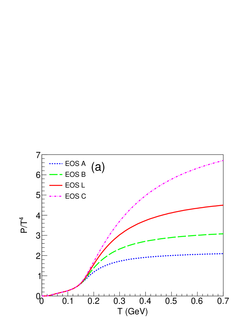
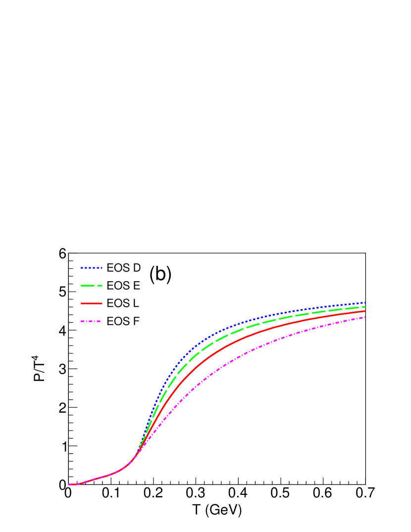
Figure 1: (Color online) The pressure $P$ normalized by $T^{4}$ versus the temperature $T$. The curves correspond to various parameterizations obtained by varying the number of degrees of freedom (a), or the transition temperature (b). The solid line in both panels, labeled ‘L’, corresponds to the lattice result Bazavov:2014pvz .

The equation of state of QCD is characterized by a transition from a hadronic, confined system at low temperatures to a phase dominated by colored degrees of freedom at high temperatures. It has been determined precisely through lattice calculations Borsanyi:2010cj ; Bazavov:2014pvz . Lattice calculations are carried out at zero baryon chemical potential, and the matter produced at central rapidity in high-energy collisions also has small net baryon number. We therefore choose to neglect net baryon density in the present study.

In lattice calculations, one first computes the trace anomaly $I\equiv\epsilon-3P$ as a function of the temperature $T$, where $\epsilon$ is the energy density and $P$ the pressure. Other quantities are then determined through the thermodynamic relations:

$$\frac{P}{T^{4}} = \int_{0}^{T}\frac{I}{T^{5}}dT,$$

$$\epsilon = I+3P,$$

$$s = \frac{\epsilon+P}{T}.$$ (6)

The equation of state used in hydrodynamic calculations is constrained, on the low-temperature side, by the condition that it matches that of the hadron resonance gas created at the end of the evolution Huovinen:2009yb ; Monnai:2015sca . All the equations of state used in this paper match the hadron resonance gas for temperatures smaller than 140 MeV, which is the freeze-out temperature of our hydrodynamic calculation. We choose to vary the high-temperature part along two different directions: either by varying the high-temperature limit of $P/T^{4}$, which is proportional to the number of degrees of freedom of the quark-gluon plasma (denoted as equation of state (EOS) A, B, L and C in Fig. 1 (a) where EOS L corresponds to the lattice QCD-based equation of state), or by varying the temperature range over which the transition occurs (denoted as equation of state (EOS) D, E, L and F in Fig. 1 (b)). The parameterization is explicated in Appendix A. We thus span a range of equations of state around the lattice value. Note that the error on $P/T^{4}$ from lattice calculations is smaller than $0.1$ for all $T$ Borsanyi:2010cj . We explore a much wider range of equations of state.

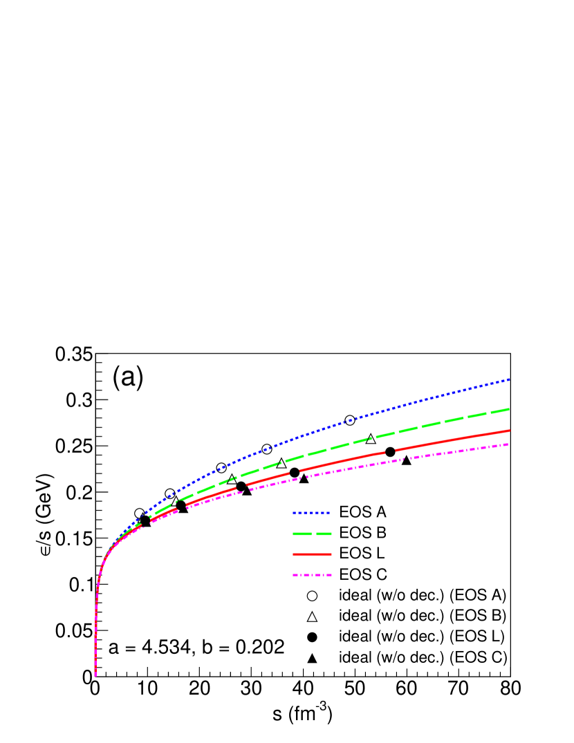
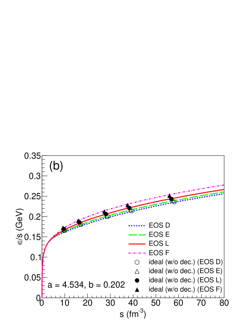
Figure 2: (Color online) Energy over entropy versus entropy density for the equations of state shown in Fig. 1. Symbols correspond to Eq. (II) where $\langle m_{T}\rangle$ and $dN/dy$ are evaluated at $T_{f}=140$ MeV in ideal hydrodynamics, before resonance decays.

According to the picture outlined in Sec. II, heavy-ion collisions measure the variation of the energy over entropy ratio as a function of the entropy density. This variation is displayed in Fig. 2 for the various equations of state displayed in Fig. 1. Note that the ratio $\epsilon/s$ is closely related to the temperature VanHove:1982vk :

$$\frac{3T}{4}<\frac{\epsilon}{s}<T,$$ (7)

where the lower bound corresponds to the ideal gas limit $P=\epsilon/3$ and the upper bound to $P=0$. Thus, the variation of $\epsilon/s$ as a function of $s$ is essentially the variation of the temperature with the entropy density. In the high-temperature phase, $s\propto\nu T^{3}$, where $\nu$ is the effective number of degrees of freedom of the quark gluon plasma. More degrees of freedom implies a smaller temperature, for the same entropy density, which explains why the order of the curves is inverted in Fig. 2 compared to Fig. 1.

IV Hydrodynamic calculations

In this section, we carry out hydrodynamical simulations in order to determine the mapping between observables and the equation of state according to Eq. (II). We model the evolution of the fluid near midrapidity and assume boost invariance in the longitudinal direction Bjorken:1982qr . We solve the transverse expansion numerically using a (2+1)-dimensional code Monnai:2014kqa . The initial transverse velocity is assumed to be zero at the proper time $\tau_{0}=0.4$ fm/c at which the hydrodynamic expansion starts. This small value of $\tau_{0}$ accounts for the early transverse expansion Ryblewski:2012rr ; vanderSchee:2013pia ; Keegan:2016cpi , irrespective of whether or not hydrodynamics is applicable at early times Vredevoogd:2008id .

Initial conditions are defined by the initial transverse density profile. The most important quantity involving initial conditions in this study is the effective radius $R_{0}$ defined by:

$$R_{0}^{2}\equiv 2\left(\langle|{\bf x}|^{2}\rangle-|\langle{\bf x}\rangle|^{2}\right),$$ (8)

where ${\bf x}$ is the position in the transverse plane, and angular brackets denote an average value weighted with the initial entropy density:

$$\langle F({\bf x})\rangle\equiv\frac{\int F({\bf x})s({\bf x},\tau_{0})d^{2}{\bf x}}{\int s({\bf x},\tau_{0})d^{2}{\bf x}}.$$ (9)

The normalization factor 2 in Eq. (8) ensures that one recovers the correct result for a uniform entropy density profile within a circle of radius $R_{0}$.

In the ideal experiment described in Sec. II, the mapping between observables and the equation of state is independent of the shape of the initial volume. For this reason, one expects that most of the dependence on the shape of the initial density profile is through the radius $R_{0}$. This has been checked in detail in studies of transverse momentum fluctuations Broniowski:2009fm ; Bozek:2012fw ; Bozek:2017jog , where it was shown that the mean transverse momentum in hydrodynamics is sensitive to initial state fluctuations only through fluctuations of $R_{0}$. We have checked it independently by comparing two standard models of initial conditions, the Monte Carlo Glauber model Miller:2007ri and the MCKLN Drescher:2006ca model, as will be explained below. The default setup of our hydrodynamic calculation uses a Monte Carlo Glauber simulation of 0-5% most central Au+Au collisions where the energy density is a sum of contributions of binary collisions, and the contribution of each collision is a Gaussian of width 0.4 fm centered half way between the colliding nucleons. The resulting density profile is centered, and then averaged over a large number of events in order to obtain a smooth profile Qiu:2011iv . The normalization of the density profile determines the multiplicity $dN/dy$. We run each calculation with 5 different normalizations spanning a range which covers the LHC and RHIC data which will be used in Sec. V.

IV.1 Ideal hydrodynamics

We first carry out ideal hydrodynamic simulations for all the equations of state displayed in Fig. 1. The fluid is converted into hadrons through the standard Cooper-Frye freeze-out procedure Cooper:1974mv at a temperature $T_{f}=140$ MeV. We include all hadron resonances with $M<2.25$ GeV, and compute $\langle m_{T}\rangle$ and $dN/dy$ directly at freeze-out, before resonances decay. Our goal here is to mimic as closely as possible the ideal experiment outlined in Sec. II.

The symbols in Fig. 2 correspond to the right-hand side of Eq. (II), where the dimensionless parameters $a$ and $b$ have been fitted to achieve the best possible agreement with the left-hand side. There are 5 points for each equation of state, which correspond to different initial temperatures. The overall agreement is excellent, and shows that the variation of $\langle m_{T}\rangle$ as a function of $(1/R_{0}^{3})(dN/dy)$ is determined by the equation of state.

In order to test that this mapping is independent of initial conditions, we have carried out a calculation with MCKLN initial conditions. While both models give values of $R_{0}$ that differ by 5%, they yield the same value of $\langle m_{T}\rangle$ when compared at the same value of $(1/R_{0}^{3})dN/dy$.

Let us now comment on the order of magnitude of the fit parameters $a$ and $b$. First, compare Eq. (3) and the second line of Eq. (II). The entropy per particle at freeze-out before decays is $(S/N)_{T_{f}}=6.5$ in this calculation. The transverse mass of a particle is smaller than its energy, since it does not include the longitudinal momentum $p_{z}$. The relevant longitudinal momentum here is that relative to the fluid, which cannot be measured, since data are integrated over all fluid rapidities. The value of $b=0.202$ is slightly larger than $(N/S)_{T_{f}}=0.154$, and thus compensates for the loss of longitudinal momentum.

We now discuss the order of magnitude of $a$. The main difference between the ideal experiment described in Sec. II and the real experiment is that the energy of the fluid slice decreases as a result of the work done by the longitudinal pressure. In ideal hydrodynamics, this cooling is only significant at early times: After the transverse expansion sets in, the pressure decreases very rapidly, the work becomes negligible and the energy stays constant. A rough, but qualitatively correct, picture is that the expansion is purely longitudinal during a time $\tau_{\rm eff}$ and that the energy is conserved for $\tau>\tau_{\rm eff}$ Ollitrault:1991xx . For dimensional reasons, $\tau_{\rm eff}=fR_{0}$, where $f$ is of order unity. The volume at $\tau_{\rm eff}$ is $V=\pi R_{0}^{2}\tau_{\rm eff}=\pi fR_{0}^{3}$. Inserting this value into Eq. (2) and identifying the right-hand side with the first line of Eq. (II), one obtains $f\simeq 0.5$, in agreement with the value obtained in previous calculations Ollitrault:1991xx . Ideal hydrodynamics thus probes the equation of state at a time $\tau_{\rm eff}\sim 0.5R_{0}$, which is the typical time at which transverse flow and elliptic flow develop Kolb:1999es ; Kolb:2000sd ; Gombeaud:2007ub .

IV.2 Resonance decays

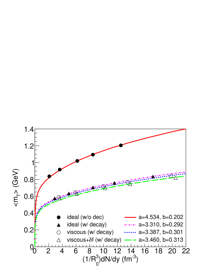
Figure 3: (Color online) Comparison of results from various hydrodynamic calculations. From top to bottom: ideal hydrodynamics before and after decays, viscous hydrodynamics without and with viscous correction at freeze-out.

The largest correction to the naive ideal fluid picture comes from decays occurring through strong or electromagnetic interactions, which occur after freeze-out, but before the daughter particles reach the detectors. We compute particle spectra after strong and electromagnetic decays, but before weak decays. Decays are treated in Ref. Sollfrank:1990qz , by assuming that the decay rate is proportional to the invariant phase space. After decays, the only remaining particles are pions, kaons, nucleons and strange baryons. In this preliminary study, we neglect strange baryons, which are a small fraction of the total number of particles, and are identified in separate analyses Abelev:2013xaa . We therefore evaluate the multiplicity $dN/dy$ and the mean transverse mass including only pions, kaons, and (anti)nucleons, both charged and neutral. As shown in Fig. 3, decays increase the multiplicity by 40%. They also conserve the total energy, so that $\langle m_{T}\rangle$ decreases, while the product $\langle m_{T}\rangle dN/dy$ only changes by a few percent.

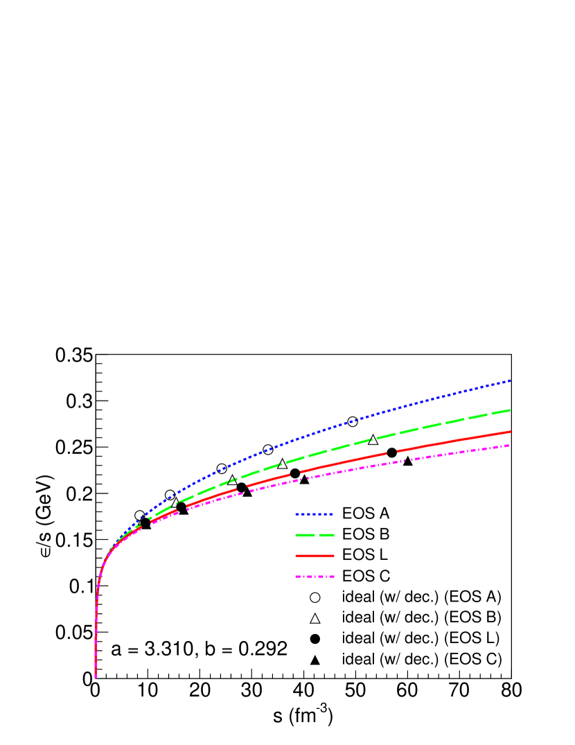
Figure 4: (Color online) Same as Fig. 2 (a) after resonance decays.

Since the increase of $dN/dy$ due to decays depends solely on the freeze-out temperature, but is independent of the colliding energy and the equation of state, decays amount to further rescalings of $\langle m_{T}\rangle$ and $dN/dy$. They can be taken into account by modifying the values of the coefficients $a$ and $b$ in Eq. (II). We again determine the values of $a$ and $b$ through a simultaneous least-square fit to all equations of state. The result is shown in Fig. 4, where only the equations of state of Fig. 7 (a) are shown. After rescaling, the effective entropy density of the fluid is unchanged: locations of symbols in Fig. 2 (a) and Fig. 4 are identical to within less than 0.5%. The fact that they are identical confirms that Eqs. (II) reconstruct thermodynamic properties of the fluid.

A more realistic description of the hadronic stage should include not only decays, but also rescatterings, for instance by coupling hydrodynamics to a transport code Teaney:2000cw ; Petersen:2008dd ; Song:2010aq . It has been recently shown Ryu:2017qzn that transverse momentum spectra are remarkably independent of the temperature at which one switches from the hydrodynamic to the transport description, which implies that our results would be unchanged if we switched from a hydrodynamic description to a transport calculation at a temperature larger than 140 MeV. Below 140 MeV, effects of hadronic scatterings are suppressed due to the lower density. Our choice of $T_{f}$ allows us to roughly reproduce observed particle ratios, in agreement with Ref. Ryu:2017qzn . This is important as the mean $m_{T}$, averaged over all particle species, strongly depends on particle ratios.

IV.3 Viscosity

We finally study viscous corrections to the ideal fluid picture. We use “minimal” shear viscosity $\eta/s=1/4\pi$ Kovtun:2004de and bulk viscosity $\zeta/s=2(1/3-c_{s}^{2})\eta/s$ Buchel:2007mf based on the gauge-string correspondence, where $c_{s}$ is the sound velocity. The relaxation times are also conjectured in the holographic approach Natsuume:2007ty . Viscosity modifies the equations of motion of the fluid Israel:1979wp , and the momentum distribution of particles at freeze-out Teaney:2003kp ; Monnai:2009ad . We show both effects separately in Fig. 3. The main effect of viscosity is to increase the multiplicity for a given initial condition, which is a consequence of the entropy increase due to dissipative processes. On the other hand, the value of $\langle m_{T}\rangle$ changes little, which is due to a partial cancellation between effects of shear viscosity (which increases $\langle m_{T}\rangle$) and bulk viscosity (which decreases $\langle m_{T}\rangle$) Monnai:2009ad .

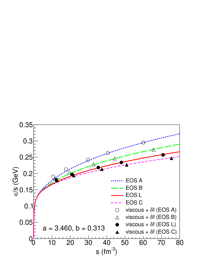
Figure 5: (Color online) Same as Fig. 4 with shear and bulk viscosity included.

The values of $\langle m_{T}\rangle$ and $dN/dy$ can again be matched to the equation of state through Eqs. (II). We again determine the values of $a$ and $b$ which give the best simultaneous fit to all equations of state. The result is displayed in Fig. 5, where only the equations of state of Fig. 7 (a) are shown. This figure shows that viscous corrections do not alter qualitatively the ideal fluid picture, and that the variation of the mean transverse mass with the multiplicity density is still driven by the equation of state in the presence of viscosity. Comparison with Fig. 4 shows that symbols are shifted to the right, which means that for the same initial temperature, viscous hydrodynamics results in a higher effective entropy density. The reason is that entropy is produced in the off-equilibrium processes.

The actual value of the shear and bulk viscosity are not known precisely. Since $a$ and $b$ depend slightly on the viscosity, the uncertainty on the viscosity translate into an uncertainty on the mapping of experimental data onto the equation of state through Eq. (II). The upper bound on constant $\eta/s$ from heavy-ion data is typically $0.2$ Shen:2015msa . It has been recently noted that the inclusion of bulk viscosity tends to lower the preferred value of the shear viscosity Ryu:2017qzn , so that $\eta/s<0.2$ seems conservative. We assume that viscous corrections are proportional to the viscosity, therefore the uncertainty can be inferred from the difference between our viscous and ideal calculations. The uncertainty on $a$ is $7\%$ and amounts on an uncertainty on the effective entropy density $s_{\rm eff}$. The uncertainty on $b$ is $11\%$ and is essentially an uncertainty on the corresponding temperature. Note, however, that the dependence on $a$ and $b$ cancels in the logarithmic slope, Eq. (5), and the ratio $P/\epsilon$ can be determined precisely even if transport coefficients are not precisely determined.

V Comparison with data

$\sqrt{s}$	$dN/dy$	$\langle m_{T}\rangle$	$R_{0}$	$s_{\rm eff}$	$T_{\rm eff}$
(GeV)		(MeV)	(fm)	(fm-3)	(MeV)
5020 Abelev:2013vea	?	?	$6.21$	$48.1\pm 3.1$	$292\pm 5$
2760 Abelev:2013vea	$2764\pm 177$	$686\pm 19$	$6.17$	$40.7\pm 2.6$	$279\pm 5$
1200 Adler:2003cb	$1146\pm 79\phantom{1}$	$589\pm 33$	$5.97$	$18.6\pm 1.3$	$227\pm 4$
1200 Abelev:2008ab	$1220\pm 97\phantom{1}$	$590\pm 48$	$5.97$	$19.9\pm 1.6$	$231\pm 5$
1130 Adams:2003xp	$1042\pm 77\phantom{1}$	$560\pm 41$	$5.93$	$17.1\pm 1.3$	$223\pm 4$
62.4 Abelev:2008ab	$\phantom{1}867\pm 65\phantom{1}$	$549\pm 28$	$5.92$	$14.3\pm 1.1$	$214\pm 4$

Table 1: Results for Pb+Pb collisions at the LHC and Au+Au collisions at RHIC. The centrality is 0-6% for 130 GeV data and 0-5% for all other energies. The first columns give our Values of $\langle m_{T}\rangle$ and $dN/dy$, obtained by extrapolating the measurements (see text). The 3rd column is the value of $R_{0}$ we use in Eq. (II), which is obtained from a Glauber model, but subject to significant theoretical uncertainty (see text). The last columns give the values of the effective entropy density defined by Eq. (II), and of the corresponding temperature if the equation of state is taken from lattice QCD. Error bars on $s_{\rm eff}$ and $T_{\rm eff}$ are experimental only.

We now discuss to what extent existing data constrain the equation of state. Both $dN/dy$ and $\langle m_{T}\rangle$ require spectra of pions, kaons and protons. Such data have been published by STAR Abelev:2008ab and PHENIX Adler:2003cb at the Relativistic Heavy Ion Collider (RHIC) and by ALICE Abelev:2013vea at the Large Hadron Collider (LHC). PHENIX and ALICE data for protons are corrected for the contamination from weak $\Lambda$ decays, while STAR data are not. We correct STAR data by assuming that a fraction $35\%\pm 10\%$ of protons come from $\Lambda$ decays, as determined by the PHENIX analysis Adler:2003cb . Particles are only identified within a limited $p_{T}$ range, which depends on the experiment, and spectra must be extrapolated in order to obtain $dN/dy$ and $\langle m_{T}\rangle$. These extrapolations are discussed in Appendix B. The data we use are for charged particles, and we need $\langle m_{T}\rangle$ and $dN/dy$ for all hadrons, including neutral ones. Yields of neutral particles are obtained assuming isospin symmetry. The resulting values of $\langle m_{T}\rangle$ and $dN/dy$ are given in Table 1. For 200 GeV, we include both STAR and PHENIX measurements, which are slightly different, but compatible within errors.

In order to convert the multiplicity $dN/dy$ into a density, one needs an estimate of the initial transverse size $R_{0}$. This quantity, which represents the mean square radius of the initial density profile, is not measured and can only be estimated in a model. As we shall see, it turns out to be the largest source of uncertainty when constraining the equation of state from data. In particular, the uncertainty from $R_{0}$ is larger than the uncertainty from transport coefficients.

We discuss how we estimate $R_{0}$. Note that the transverse size fluctuates event to event, even in a narrow centrality window Broniowski:2009fm . Ideally, we would like to estimate the average value over events of $(1/R_{0}^{3})dN/dy$. Since the input available from experiment is an average of $dN/dy$, for the sake of simplicity, we estimate the average value of $R_{0}$ over many events to divide $dN/dy$ for our analyses. We use the same Monte Carlo Glauber model as in our hydrodynamic calculation. The resulting values, averaged over many events, are given in Table 1. The MCKLN model Drescher:2006ca gives values $5\%$ smaller, which implies that the density is $15\%$ larger. This shows that the uncertainty on the transverse size is significant.

However, the variation of $R_{0}$ with colliding energy for a given system is small, so that the evolution of the density is mostly driven by the increase in the multiplicity $dN/dy$. Therefore, uncertainties on $R_{0}$ cancel when comparing two different collision energies. The variation of the mean transverse mass with $dN/dy$ directly gives the ratio $P/\epsilon$, as shown by Eq. (5). As pointed out in Sec. IV.3, uncertainties from the viscosity also cancel in this energy dependence. Using PHENIX and ALICE data, which span a wide range of $dN/dy$, and taking into account the different sizes of Au and Pb nuclei, Eq. (5) gives

$$\left.\frac{P}{\epsilon}\right|_{T_{\rm eff}}=0.21\pm 0.10,$$ (10)

where the error is solely from experiment.

The only significant theoretical uncertainty is on the effective temperature $T_{\rm eff}$ at which this ratio is measured. We provide in Table 1 the values of the effective entropy density $s_{\rm eff}$ given by Eq. (II), where $a$ is given by our viscous hydrodynamic calculation. The value at $5.02$ TeV, where identified particle spectra are not yet published, is obtained by assuming that the relative increase in $dN/dy$ from $2.76$ TeV equals that of $dN_{\mathrm{ch}}/d\eta$, that is, 20% Adam:2015ptt . As discussed in Sec. IV.3, the uncertainty on $s_{\rm eff}$ from transport coefficients is $7\%$, and that from the transverse size $R_{0}$ is at least 15%.

The value of the temperature $T_{\rm eff}$ corresponding to $s_{\rm eff}$ can only be obtained if the equation of state is known. The values in the last column of Table 1 correspond to the lattice equation of state. Lattice calculations give $P/\epsilon=0.23$ for a temperature half-way between the values of $T_{\rm eff}$ corresponding to 200 GeV and 2.76 TeV. The experimental value, Eq. (10), is compatible with the lattice result. Experiments at $\sqrt{s}=5.02$ TeV, for which identified particle spectra are yet unpublished, will probe the equation of state at a temperature close to 300 MeV. Note that the theoretical uncertainty of $\simeq 20\%$ on $s_{\rm eff}$ translates into an uncertainty $\sim 15$ MeV on the effective temperature at the LHC, which is dominated by the uncertainty on the initial transverse radius $R_{0}$.

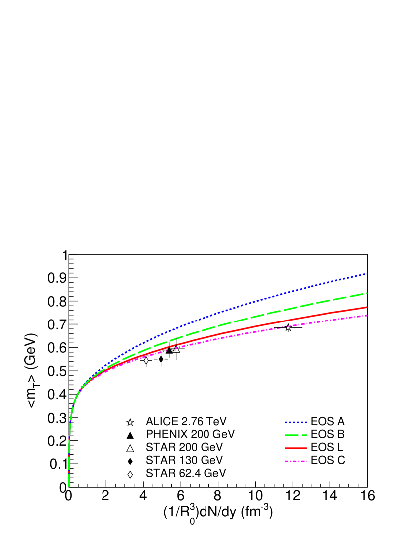
Figure 6: (Color online) Experimental data from Table 1, compared to value given by various equations of state and Eqs. (II), where $a$ and $b$ are taken from our viscous hydrodynamic calculation, and $R_{0}$ from a Glauber model (see text).

Figure 6 shows the comparison between experimental data and the values obtained from the equation of state through Eqs. (II), where $a$ and $b$ are taken from our viscous hydrodynamic calculation (see Fig. 5). With the minimal viscosity chosen in this calculation, LHC data slightly favor the equation of state C, which has a larger pressure than the lattice equation of state. With a higher viscosity, however, the lattice equation of state would be preferred. Equations of state A and B are ruled out: as already well known, heavy-ion data favor a soft equation of state. Note that current experiments only probe the equation of state up to $T\sim 300$ MeV (see Table 1).

VI Conclusions

We have shown that in central nucleus-nucleus collisions, the variation of the mean transverse mass as a function of the multiplicity density is, up to rescaling factors, driven by the variation of the energy over entropy ratio $\epsilon/s$ as a function of the entropy density $s$. Each collision energy probes the equation of state at a different entropy density $s_{\rm eff}$, which corresponds roughly to the average density at a time $\tau_{\rm eff}\sim 3$ fm/$c$. RHIC and LHC experiments probe the equation of state for temperatures up to $\sim 300$ MeV.

The largest source of uncertainty at the theoretical level is the initial transverse size $R_{0}$. The uncertainty from unknown transport coefficients (shear and bulk viscosity) is twice smaller. These theoretical uncertainties cancel if one measures the evolution of the mean transverse mass as a function of collision energy, which gives direct access to the pressure over energy density ratio $P/\epsilon$ of the quark-gluon plasma.

This analysis requires precise experimental data on identified particle spectra. One could think of replacing the transverse mass with the transverse momentum, and the rapidity by the pseudorapidity, which was the original idea of Van Hove VanHove:1982vk , and would allow to work with unidentified particles. However, we have checked that the mapping onto the equation of state is not as good in this case.

The value of $P/\epsilon$ obtained from the evolution of spectra from RHIC to LHC energies is compatible with the lattice equation of state, but with large errors. Carrying out an energy scan at the LHC with a single detector would greatly improve the quality of the measurement.

Appendix A Varying the equation of state

The equation of state is constructed by connecting the trace anomaly of the hadron resonance gas model smoothly to that of lattice QCD Bazavov:2014pvz . To systematically generate variations of the equation of state, modification is made through two factors $c_{w}$ and $c_{h}$ in the QGP phase for our analyses. The expression reads:

$$I(T) = \frac{1}{2}\bigg{[}1-\tanh\bigg{(}\frac{T-T_{s}}{\Delta T_{s}}\bigg{)}\bigg{]}I_{\mathrm{HRG}}(T)$$ (11)

$$+ \frac{c_{h}}{2}\bigg{[}1+\tanh\bigg{(}\frac{T-T_{s}}{\Delta T_{s}}\bigg{)}\bigg{]}I_{\mathrm{lat}}(T_{w}),$$

where $T_{w}=T_{s}+c_{w}(T-T_{s})$. $c_{w}$ and $c_{h}$ are associated with the width and the magnitude of $I(T)$ in the QGP phase, respectively. $c_{w}=1$ and $c_{h}=1$ recover the lattice QCD result. The hadronic equation of state is left untouched because, as mentioned earlier, the Cooper-Frye formula requires that kinetic theory reproduces the equation of state used in the hydrodynamic model at freeze-out for energy-momentum conservation. When one chooses $T_{s}=160$ MeV and $\Delta T_{s}=0.1T_{s}$, this is satisfied at and below $T=140$ GeV.

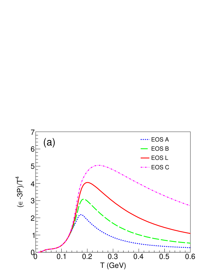
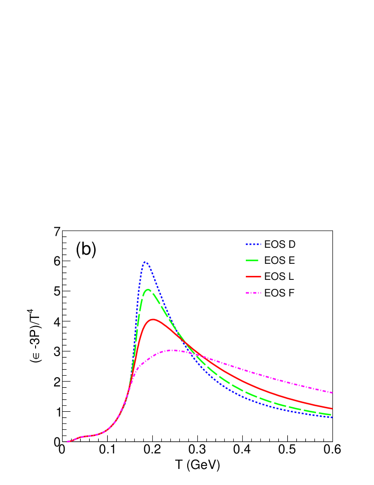
Figure 7: (Color online) The trace anomaly normalized by $T^{4}$ versus the temperature $T$. The curves correspond to various parameterizations obtained by varying the number of degrees of freedom (a), or the transition temperature (b).

The pressure is obtained through the thermodynamic relations (III). Since the trace anomaly is integrated, $c_{w}$ and $c_{h}$ have to be modified simultaneously to shift the pseudo-critical temperature and change the effective number of degrees of freedom in the pressure or the entropy density (Fig.7).

We first consider a set of equation of state with different numbers of QGP degrees of freedom by choosing $(c_{w},c_{h})$ = $(2,0.5)$, $(1.5,0.75)$, $(1,1)$, and $(0.5,1.25)$. They are labeled as EOS A, B, L and C, respectively. The normalized pressure as a function of the temperature for each equation of state is plotted in Fig. 1 (a). It is note-worthy that we consider an equation of state which exceeds the Stefan-Boltzmann limit with the last parameter set $(0.5,1.25)$. We also vary the pseudo-critical temperature by setting the parameters to $(c_{w},c_{h})$ = $(2,1.5)$, $(1.5,1.25)$, $(1,1)$, and $(0.5,0.75)$ as shown in Fig. 1 (b), which are labeled as EOS D, E, L and F. The equation of state becomes harder for larger $T_{c}$ because it is fixed on the hadronic side.

Appendix B Identified particle spectra at RHIC and LHC

In order to estimate the mean transverse mass per particle from experimental data, we use as input $p_{T}$ spectra of identified charged hadrons in the central rapidity region. More specifically, we use data for charged pions, charged kaons, protons and antiprotons, which are shown as symbols in Fig. 8. These plots show the probability distribution of $p_{T}$ near midrapidity, $dN/dp_{T}dy$. Experimental data are shown as symbols. Pion and kaon yields increase smoothly with collision energy as expected. This does not appear to hold for proton and antiprotons, but the reason is simply that STAR data for protons and antiprotons include, in addition to primary particles, secondary products of weak $\Lambda$ and $\bar{\Lambda}$ decays. Apart from this difference, PHENIX and STAR data at 200 GeV are compatible within error bars.

The effect of the net baryon number becomes visible at the lower energies: it results in more protons than antiprotons at midrapidity, and also slightly more $K^{+}$ than $K^{-}$ because the strangeness chemical potential is non-vanishing in the presence of the net baryon chemical potential $\mu_{B}$ owing to the strangeness neutrality condition. While the differences between particles and antiparticles are linear in $\mu_{B}$, the total multiplicities are even functions of $\mu_{B}$, hence effects of net baryon number only appear to order $\mu_{B}^{2}$. We assume that they are negligible down to 62.4 GeV.

Particles are identified only in a limited $p_{T}$ range which depends on the experiment. In order to evaluate the mean $m_{T}$, we need to extrapolate the measured spectrum to the whole $p_{T}$ range. These extrapolations are done with blast-wave fits Schnedermann:1993ws . For ALICE data, we fit each particle species independently, as in the experimental paper Abelev:2013vea . The resulting values of $dN/dy$ and $\langle p_{T}\rangle$ are given in Tables 2 and 3. They are very close to the values in the experimental paper. The small differences, which are much smaller than error bars, can be ascribed to different fitting algorithms. For sake of consistency, we also use blast-wave fits to extrapolate PHENIX data Adler:2003cb . The resulting values of $dN/dy$ and $\langle p_{T}\rangle$ differ somewhat from the experimental values which use a different extrapolation scheme, but are compatible within error bars. For STAR data, the $p_{T}$ range is too limited to fit each particle species independently: therefore, we follow the recommendation of the experimental paper Abelev:2008ab and carry out a simultaneous fit for kaons and (anti)protons. For pions, however, we carry out an independent blast-wave fit as for PHENIX data. Agreement between STAR and PHENIX pion yields at 200 GeV is much better than in the corresponding experimental papers, which suggests that the differences were mostly due to the different extrapolation methods.

Finally, the values of $\langle m_{T}\rangle$, which are needed in this paper, are listed in Table 4.

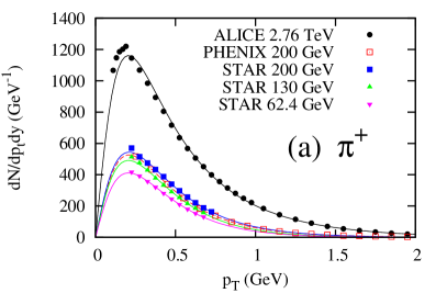
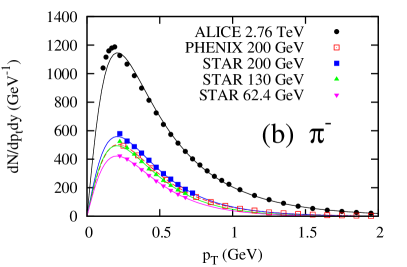
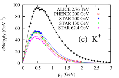
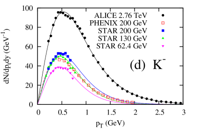
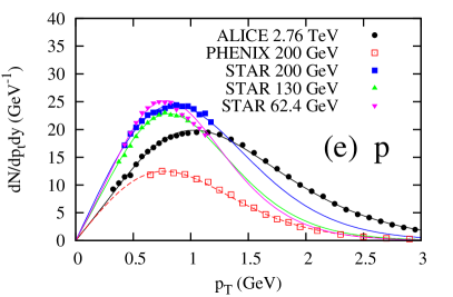
Figure 8: (Color online) Transverse momentum distributions of identified particles in Pb+Pb collisions at the LHC and Au+Au collisions at RHIC. The centrality range is 0-5% for all sets of data except 130 GeV data which are 0-6%. Symbols are data from ALICE Abelev:2013vea , PHENIX Adler:2003cb and STAR Adams:2003xp ; Abelev:2008ab . Solid lines are blast-wave fits (see text). Each panel corresponds to a different particle species: positive (a) and negative (b) pions, positive (c) and negative (d) kaons, protons (e) and antiprotons (f). STAR data for protons and antiprotons also include secondary products of $\Lambda$ and $\bar{\Lambda}$ decays, which explain the larger values. Experimental errors are not shown for sake of readability, but they are taken into account in the fits.

exp.	$\sqrt{s}$ [GeV]	$\pi^{+}$		$\pi^{-}$		$K^{+}$		$K^{-}$		$p$		$\bar{p}$
ALICE	2760	732.3	733$\pm$54	731.0	732$\pm$52	109.0	109$\pm$9	108.6	109$\pm$9	33.6	34$\pm$3	33.2	33$\pm$3
PHENIX	200	306.5	286.4$\pm$24.2	297.6	281.8$\pm$22.8	48.1	48.9$\pm$6.3	43.8	45.7$\pm$5.2	16.4	18.4$\pm$2.6	11.7	13.5$\pm$1.8
STAR	200	310.6	322$\pm$25	315.1	327$\pm$25	51.3	51.3$\pm$6.5	49.2	49.6$\pm$6.2	34.5	34.7$\pm$4.4	27.7	26.7$\pm$3.4
STAR	130	265.5	278$\pm$20	267.7	280$\pm$20	46.7	46.3$\pm$3.0	43.1	42.7$\pm$2.8	28.2	28.2$\pm$3.1	19.9	20.2$\pm$2.2
STAR	62.4	221.1	233$\pm$17	225.2	237$\pm$17	38.3	37.6$\pm$2.7	32.5	32.4$\pm$2.3	29.2	29.0$\pm$3.8	13.5	13.6$\pm$1.7

Table 2: Values of $dN/dy$ for identified hadrons obtained by extrapolating measured spectra to the whole $p_{T}$ range. Our extrapolations are compared with the extrapolations done by experimental collaborations (in italics).

exp.	$\sqrt{s}$ [GeV]	$\pi^{+}$		$\pi^{-}$		$K^{+}$		$K^{-}$		$p$		$\bar{p}$
ALICE	2760	522	517$\pm$19	525	520$\pm$18	878	876$\pm$26	867	867$\pm$27	1357	1333$\pm$33	1356	1353$\pm$34
PHENIX	200	438	451$\pm$33	447	455$\pm$32	681	670$\pm$78	697	677$\pm$68	1021	949$\pm$85	1051	959$\pm$84
STAR	200	443	427$\pm$22	437	422$\pm$22	720	720$\pm$74	720	719$\pm$74	1102	1104$\pm$110	1102	1103$\pm$114
STAR	130	414	404$\pm$13	415	404$\pm$13	668	666$\pm$30	668	667$\pm$30	1002	1003$\pm$87	1002	1002$\pm$87
STAR	62.4	410	406$\pm$11	407	403$\pm$11	646	646$\pm$29	646	645$\pm$29	960	956$\pm$75	960	959$\pm$60

Table 3: Values of $\langle p_{t}\rangle$ (in MeV/$c$) for identified hadrons obtained by extrapolating measured spectra to the whole $p_{T}$ range. Our extrapolations are compared with the extrapolations done by experimental collaborations (in italics).

exp.	$\sqrt{s}$ [GeV]	$\pi^{+}$	$\pi^{-}$	$K^{+}$	$K^{-}$	$p$	$\bar{p}$
ALICE	2760	553	555	1043	1034	1702	1702
PHENIX	200	472	481	878	889	1435	1455
STAR	200	475	470	906	906	1496	1496
STAR	130	448	449	861	861	1416	1416
STAR	62.4	444	441	843	843	1384	1384

Table 4: Values of $\langle m_{t}\rangle$ (in MeV) for identified hadrons obtained by extrapolating measured spectra to the whole $p_{T}$ range.

References

- (1) H. Stoecker and W. Greiner, Phys. Rept. 137, 277 (1986). doi:10.1016/0370-1573(86)90131-6
- (2) L. G. Yaffe and B. Svetitsky, Phys. Rev. D 26, 963 (1982). doi:10.1103/PhysRevD.26.963
- (3) F. R. Brown, F. P. Butler, H. Chen, N. H. Christ, Z. h. Dong, W. Schaffer, L. I. Unger and A. Vaccarino, Phys. Rev. Lett. 65, 2491 (1990). doi:10.1103/PhysRevLett.65.2491
- (4) Y. Aoki, G. Endrodi, Z. Fodor, S. D. Katz and K. K. Szabo, Nature 443, 675 (2006) doi:10.1038/nature05120 [hep-lat/0611014].
- (5) P. de Forcrand and O. Philipsen, JHEP 0701, 077 (2007) doi:10.1088/1126-6708/2007/01/077 [hep-lat/0607017].
- (6) Z. Fodor and S. D. Katz, JHEP 0404, 050 (2004) doi:10.1088/1126-6708/2004/04/050 [hep-lat/0402006].
- (7) K. Fukushima and T. Hatsuda, Rept. Prog. Phys. 74, 014001 (2011) doi:10.1088/0034-4885/74/1/014001 [arXiv:1005.4814 [hep-ph]].
- (8) S. Borsanyi, G. Endrodi, Z. Fodor, A. Jakovac, S. D. Katz, S. Krieg, C. Ratti and K. K. Szabo, JHEP 1011, 077 (2010) doi:10.1007/JHEP11(2010)077 [arXiv:1007.2580 [hep-lat]].
- (9) A. Bazavov et al. [HotQCD Collaboration], Phys. Rev. D 90, 094503 (2014) doi:10.1103/PhysRevD.90.094503 [arXiv:1407.6387 [hep-lat]].
- (10) C. Gale, S. Jeon and B. Schenke, Int. J. Mod. Phys. A 28, 1340011 (2013) doi:10.1142/S0217751X13400113 [arXiv:1301.5893 [nucl-th]].
- (11) P. F. Kolb and U. W. Heinz, In *Hwa, R.C. (ed.) et al.: Quark gluon plasma* 634-714 [nucl-th/0305084].
- (12) P. Huovinen and P. V. Ruuskanen, Ann. Rev. Nucl. Part. Sci. 56, 163 (2006) doi:10.1146/annurev.nucl.54.070103.181236 [nucl-th/0605008].
- (13) P. Romatschke, Int. J. Mod. Phys. E 19, 1 (2010) doi:10.1142/S0218301310014613 [arXiv:0902.3663 [hep-ph]].
- (14) U. Heinz and R. Snellings, Ann. Rev. Nucl. Part. Sci. 63, 123 (2013) doi:10.1146/annurev-nucl-102212-170540 [arXiv:1301.2826 [nucl-th]].
- (15) M. Luzum and P. Romatschke, Phys. Rev. C 78, 034915 (2008) Erratum: [Phys. Rev. C 79, 039903 (2009)] doi:10.1103/PhysRevC.78.034915, 10.1103/PhysRevC.79.039903 [arXiv:0804.4015 [nucl-th]].
- (16) V. Roy and A. K. Chaudhuri, DAE Symp. Nucl. Phys. 55, 624 (2010) [arXiv:1003.1195 [nucl-th]].
- (17) I. A. Karpenko and Y. M. Sinyukov, Phys. Rev. C 81, 054903 (2010) doi:10.1103/PhysRevC.81.054903 [arXiv:1004.1565 [nucl-th]].
- (18) H. Holopainen, H. Niemi and K. J. Eskola, Phys. Rev. C 83, 034901 (2011) doi:10.1103/PhysRevC.83.034901 [arXiv:1007.0368 [hep-ph]].
- (19) H. Petersen, G. Y. Qin, S. A. Bass and B. Muller, Phys. Rev. C 82, 041901 (2010) doi:10.1103/PhysRevC.82.041901 [arXiv:1008.0625 [nucl-th]].
- (20) B. Schenke, S. Jeon and C. Gale, Phys. Rev. Lett. 106, 042301 (2011) doi:10.1103/PhysRevLett.106.042301 [arXiv:1009.3244 [hep-ph]].
- (21) T. Hirano, P. Huovinen and Y. Nara, Phys. Rev. C 83, 021902 (2011) doi:10.1103/PhysRevC.83.021902 [arXiv:1010.6222 [nucl-th]].
- (22) H. Song, S. A. Bass, U. Heinz, T. Hirano and C. Shen, Phys. Rev. Lett. 106, 192301 (2011) Erratum: [Phys. Rev. Lett. 109, 139904 (2012)] doi:10.1103/PhysRevLett.106.192301, 10.1103/PhysRevLett.109.139904 [arXiv:1011.2783 [nucl-th]].
- (23) P. Bozek, Phys. Rev. C 85, 034901 (2012) doi:10.1103/PhysRevC.85.034901 [arXiv:1110.6742 [nucl-th]].
- (24) L. Pang, Q. Wang and X. N. Wang, Phys. Rev. C 86, 024911 (2012) doi:10.1103/PhysRevC.86.024911 [arXiv:1205.5019 [nucl-th]].
- (25) Y. Akamatsu, S. i. Inutsuka, C. Nonaka and M. Takamoto, J. Comput. Phys. 256, 34 (2014) doi:10.1016/j.jcp.2013.08.047 [arXiv:1302.1665 [nucl-th]].
- (26) T. Epelbaum and F. Gelis, Phys. Rev. Lett. 111, 232301 (2013) doi:10.1103/PhysRevLett.111.232301 [arXiv:1307.2214 [hep-ph]].
- (27) A. Kurkela and Y. Zhu, Phys. Rev. Lett. 115, no. 18, 182301 (2015) doi:10.1103/PhysRevLett.115.182301 [arXiv:1506.06647 [hep-ph]].
- (28) J. P. Blaizot, F. Gelis, J. F. Liao, L. McLerran and R. Venugopalan, Nucl. Phys. A 873, 68 (2012) doi:10.1016/j.nuclphysa.2011.10.005 [arXiv:1107.5296 [hep-ph]].
- (29) J. P. Blaizot, B. Wu and L. Yan, Nucl. Phys. A 930, 139 (2014) doi:10.1016/j.nuclphysa.2014.07.041 [arXiv:1402.5049 [hep-ph]].
- (30) A. Monnai and B. Müller, arXiv:1403.7310 [hep-ph].
- (31) D. M. Dudek, W. L. Qian, C. Wu, O. Socolowski, S. S. Padula, G. Krein, Y. Hama and T. Kodama, arXiv:1409.0278 [nucl-th].
- (32) J. S. Moreland and R. A. Soltz, Phys. Rev. C 93, no. 4, 044913 (2016) doi:10.1103/PhysRevC.93.044913 [arXiv:1512.02189 [nucl-th]].
- (33) S. Pratt, E. Sangaline, P. Sorensen and H. Wang, Phys. Rev. Lett. 114, 202301 (2015) doi:10.1103/PhysRevLett.114.202301 [arXiv:1501.04042 [nucl-th]].
- (34) E. Sangaline and S. Pratt, Phys. Rev. C 93, no. 2, 024908 (2016) doi:10.1103/PhysRevC.93.024908 [arXiv:1508.07017 [nucl-th]].
- (35) L. G. Pang, K. Zhou, N. Su, H. Petersen, H. Stöcker and X. N. Wang, arXiv:1612.04262 [hep-ph].
- (36) J. P. Blaizot and J. Y. Ollitrault, Phys. Lett. B 191, 21 (1987). doi:10.1016/0370-2693(87)91314-1
- (37) F. Cooper and G. Frye, Phys. Rev. D 10, 186 (1974). doi:10.1103/PhysRevD.10.186
- (38) L. Van Hove, Phys. Lett. 118B, 138 (1982). doi:10.1016/0370-2693(82)90617-7
- (39) R. Campanini, G. Ferri and G. Ferri, Phys. Lett. B 703, 237 (2011) doi:10.1016/j.physletb.2011.08.009 [arXiv:1106.2008 [hep-ph]].
- (40) P. Ghosh and S. Muhuri, arXiv:1406.5811 [hep-ph].
- (41) J. D. Bjorken, Phys. Rev. D 27, 140 (1983). doi:10.1103/PhysRevD.27.140
- (42) J. Y. Ollitrault, Phys. Lett. B 273, 32 (1991). doi:10.1016/0370-2693(91)90548-5
- (43) P. Bozek and W. Broniowski, Phys. Rev. C 85, 044910 (2012) doi:10.1103/PhysRevC.85.044910 [arXiv:1203.1810 [nucl-th]].
- (44) J. Noronha-Hostler, M. Luzum and J. Y. Ollitrault, Phys. Rev. C 93, no. 3, 034912 (2016) doi:10.1103/PhysRevC.93.034912 [arXiv:1511.06289 [nucl-th]].
- (45) P. Huovinen and P. Petreczky, Nucl. Phys. A 837, 26 (2010) doi:10.1016/j.nuclphysa.2010.02.015 [arXiv:0912.2541 [hep-ph]].
- (46) A. Monnai and B. Schenke, Phys. Lett. B 752, 317 (2016) doi:10.1016/j.physletb.2015.11.063 [arXiv:1509.04103 [nucl-th]].
- (47) A. Monnai, Phys. Rev. C 90, no. 2, 021901 (2014) doi:10.1103/PhysRevC.90.021901 [arXiv:1403.4225 [nucl-th]].
- (48) R. Ryblewski and W. Florkowski, Phys. Rev. C 85, 064901 (2012) doi:10.1103/PhysRevC.85.064901 [arXiv:1204.2624 [nucl-th]].
- (49) W. van der Schee, P. Romatschke and S. Pratt, Phys. Rev. Lett. 111, no. 22, 222302 (2013) doi:10.1103/PhysRevLett.111.222302 [arXiv:1307.2539 [nucl-th]].
- (50) L. Keegan, A. Kurkela, A. Mazeliauskas and D. Teaney, JHEP 1608, 171 (2016) doi:10.1007/JHEP08(2016)171 [arXiv:1605.04287 [hep-ph]].
- (51) J. Vredevoogd and S. Pratt, Phys. Rev. C 79, 044915 (2009) doi:10.1103/PhysRevC.79.044915 [arXiv:0810.4325 [nucl-th]].
- (52) W. Broniowski, M. Chojnacki and L. Obara, Phys. Rev. C 80, 051902 (2009) doi:10.1103/PhysRevC.80.051902 [arXiv:0907.3216 [nucl-th]].
- (53) P. Bozek, W. Broniowski and S. Chatterjee, arXiv:1707.04420 [nucl-th].
- (54) M. L. Miller, K. Reygers, S. J. Sanders and P. Steinberg, Ann. Rev. Nucl. Part. Sci. 57, 205 (2007) doi:10.1146/annurev.nucl.57.090506.123020 [nucl-ex/0701025].
- (55) H.-J. Drescher and Y. Nara, Phys. Rev. C 75, 034905 (2007) doi:10.1103/PhysRevC.75.034905 [nucl-th/0611017].
- (56) Z. Qiu and U. W. Heinz, Phys. Rev. C 84, 024911 (2011) doi:10.1103/PhysRevC.84.024911 [arXiv:1104.0650 [nucl-th]].
- (57) P. F. Kolb, J. Sollfrank, P. V. Ruuskanen and U. W. Heinz, Nucl. Phys. A 661, 349 (1999) doi:10.1016/S0375-9474(99)85038-6 [nucl-th/9907025].
- (58) P. F. Kolb, J. Sollfrank and U. W. Heinz, Phys. Rev. C 62, 054909 (2000) doi:10.1103/PhysRevC.62.054909 [hep-ph/0006129].
- (59) C. Gombeaud and J. Y. Ollitrault, Phys. Rev. C 77, 054904 (2008) doi:10.1103/PhysRevC.77.054904 [nucl-th/0702075].
- (60) J. Sollfrank, P. Koch and U. W. Heinz, Phys. Lett. B 252, 256 (1990). doi:10.1016/0370-2693(90)90870-C
- (61) B. B. Abelev et al. [ALICE Collaboration], Phys. Rev. Lett. 111, 222301 (2013) doi:10.1103/PhysRevLett.111.222301 [arXiv:1307.5530 [nucl-ex]].
- (62) D. Teaney, J. Lauret and E. V. Shuryak, Phys. Rev. Lett. 86, 4783 (2001) doi:10.1103/PhysRevLett.86.4783 [nucl-th/0011058].
- (63) H. Petersen, J. Steinheimer, G. Burau, M. Bleicher and H. Stocker, Phys. Rev. C 78, 044901 (2008) doi:10.1103/PhysRevC.78.044901 [arXiv:0806.1695 [nucl-th]].
- (64) H. Song, S. A. Bass and U. Heinz, Phys. Rev. C 83, 024912 (2011) doi:10.1103/PhysRevC.83.024912 [arXiv:1012.0555 [nucl-th]].
- (65) S. Ryu, J. F. Paquet, C. Shen, G. Denicol, B. Schenke, S. Jeon and C. Gale, arXiv:1704.04216 [nucl-th].
- (66) P. Kovtun, D. T. Son and A. O. Starinets, Phys. Rev. Lett. 94, 111601 (2005) doi:10.1103/PhysRevLett.94.111601 [hep-th/0405231].
- (67) A. Buchel, Phys. Lett. B 663, 286 (2008) doi:10.1016/j.physletb.2008.03.069 [arXiv:0708.3459 [hep-th]].
- (68) M. Natsuume and T. Okamura, Phys. Rev. D 77, 066014 (2008) Erratum: [Phys. Rev. D 78, 089902 (2008)] doi:10.1103/PhysRevD.78.089902, 10.1103/PhysRevD.77.066014 [arXiv:0712.2916 [hep-th]].
- (69) W. Israel and J. M. Stewart, Annals Phys. 118, 341 (1979). doi:10.1016/0003-4916(79)90130-1
- (70) D. Teaney, Phys. Rev. C 68, 034913 (2003) doi:10.1103/PhysRevC.68.034913 [nucl-th/0301099].
- (71) A. Monnai and T. Hirano, Phys. Rev. C 80, 054906 (2009) doi:10.1103/PhysRevC.80.054906 [arXiv:0903.4436 [nucl-th]].
- (72) C. Shen and U. Heinz, Nucl. Phys. News 25, no. 2, 6 (2015) doi:10.1080/10619127.2015.1006502 [arXiv:1507.01558 [nucl-th]].
- (73) B. I. Abelev et al. [STAR Collaboration], Phys. Rev. C 79, 034909 (2009) doi:10.1103/PhysRevC.79.034909 [arXiv:0808.2041 [nucl-ex]].
- (74) S. S. Adler et al. [PHENIX Collaboration], Phys. Rev. C 69, 034909 (2004) doi:10.1103/PhysRevC.69.034909 [nucl-ex/0307022].
- (75) B. Abelev et al. [ALICE Collaboration], Phys. Rev. C 88, 044910 (2013) doi:10.1103/PhysRevC.88.044910 [arXiv:1303.0737 [hep-ex]].
- (76) J. Adams et al. [STAR Collaboration], Phys. Rev. Lett. 92, 112301 (2004) doi:10.1103/PhysRevLett.92.112301 [nucl-ex/0310004].
- (77) J. Adam et al. [ALICE Collaboration], Phys. Rev. Lett. 116, no. 22, 222302 (2016) doi:10.1103/PhysRevLett.116.222302 [arXiv:1512.06104 [nucl-ex]].
- (78) E. Schnedermann, J. Sollfrank and U. W. Heinz, Phys. Rev. C 48, 2462 (1993) doi:10.1103/PhysRevC.48.2462 [nucl-th/9307020].