Quantum Walks, Weyl equation and the Lorentz group

Abstract

Quantum cellular automata and quantum walks provide a framework for the foundations of quantum field theory, since the equations of motion of free relativistic quantum fields can be derived as the small wave-vector limit of quantum automata and walks starting from very general principles. The intrinsic discreteness of this framework is reconciled with the continuous Lorentz symmetry by reformulating the notion of inertial reference frame in terms of the constants of motion of the quantum walk dynamics. In particular, among the symmetries of the quantum walk which recovers the Weyl equation—the so called Weyl walk—one finds a non linear realisation of the Poincaré group, which recovers the usual linear representation in the small wave-vector limit.

In this paper we characterise the full symmetry group of the Weyl walk which is shown to be a non linear realization of a group which is the semidirect product of the Poincaré group and the group of dilations.

I Introduction

The conjecture, originally advanced by Feynman Feynman (1982), that the laws of physics can be ultimately modelled by finite algorithms is a very inspirational proposal Lloyd (2006). There are many reasons why this might prove to be the case and, thus, for adopting this conjecture as a standpoint for a research program. The primary reason is stated by Feynman himself: “It always bothers me that according to the laws as we understand them today, it takes a computing machine an infinite number of logical operations to figure out what goes on in no matter how tiny a region of space and no matter how tiny a region of time”. A similar concern is that in an arbitrarily small region of a continuous space-time it is in principle possible to store an infinite amount of bits of information. The only alternative to this situation is that the dynamics of systems in a finite region of space-time is perfectly computed by a finite algorithm running on a finite memory. Furthermore, the idea that the dynamical laws could be reconstructed within a (quantum) computational framework appears as a natural continuation of the research on quantum foundations from the information perspective (see e.g. Refs. Hardy (2001); Fuchs (2002); Chiribella et al. (2011); Dakic and Brukner (2011) and for a comprehensive historical overview see Refs.Khrennikov and Weihs (2012); Khrennikov et al. (2015); D’Ariano and Khrennikov (2016)).

As long as we accept that the best microscopic theory at our disposal is quantum theory, the most natural computational model for the description of physical laws is a quantum cellular automaton Feynman (1982); Schumacher and Werner (2004); Gross et al. (2012). The approach to the foundations of quantum field theory based on quantum cellular automata was explored for various decades Bialynicki-Birula (1994); Meyer (1996, 2001); Yepez (2006) and it is gathering increasing interest Arrighi et al. (2014a); Arnault and Debbasch (2016); Arrighi et al. (2014b); Arnault et al. (2016). Nevertheless, the idea that a discrete quantum computer can exactly compute the evolution of elementary physical systems is seemingly at clash with continuous symmetries Snyder (1947).

In recent years, free relativistic field equations were derived starting from the requirements of homogeneity, locality, linearity and isotropy D’Ariano (2011); D’Ariano and Perinotti (2014); Bisio et al. (2015, 2016a). The free quantum field theory (Weyl, Dirac, and Maxwell) is achieved by restricting to evolutions that are linear in the field–i.e. a quantum walk–in the limit of small wave-vectors, namely for states so delocalised that the discrete underlying structure cannot be resolved. It is remarkable that Lorentz-invariant equations can be derived without imposing the relativity principle, and not even mechanical notions. However, the Lorentz symmetry has no direct interpretation in the above framework, where the geometry of space-time is not assumed a priori. The achievement of Weyl, Dirac and Maxwell’s equations is a clear indication that an alleged conflict between discrete dynamics and continuous symmetries was drawn based only on naive intuition.

In Ref. Bisio et al. (2016b) the notion of inertial reference frame has been formulated in terms of representation of the dynamics parameterised by the values of the constants of motion. Such notion is suitable to the study of dynamical symmetries, without the need of resorting to a space-time background. In this way the Galileo principle of relativity is formulated by identifying the notion of change of inertial frame with the change of representation that leaves the eigenvalue equation of the quantum walk invariant. In the same Ref. Bisio et al. (2016b) it has been shown that such changes of representations for the Weyl quantum walk encompass a non-linear realization of the Poincaré group. This result, besides embodying a microscopic model of Doubly Special Relativity (DSR) Amelino-Camelia and Piran (2001); Magueijo and Smolin (2002); Amelino-Camelia et al. (2011), represents a proof of principle of the coexistence of a discrete quantum dynamics with the symmetries of classical space-time.

In this paper we review and extend the results of Ref. Bisio et al. (2016b) classifying the full symmetry group of the Weyl quantum walk, which is a semidirect product of the group of diffeomorphic dilations of the null mass shell by the Poincaré group.

II Weyl quantum walk

A quantum cellular automaton gives the evolution of a denumerable set of cells, each one corresponding to a quantum system. We consider the case in which each quantum system is described by the algebra generated by a set of field operators. Following the definition of Ref.Schumacher and Werner (2004), a quantum cellular automaton is an automorphism of the quasi-local algebra. The restriction to non interacting dynamics corresponds to consider algebra automorphism that are linear in the field operators (i.e. each field operator is mapped to a linear combination of field operators). In the same way the dynamics of a free field is specified by its single particle sector, a linear quantum cellular automaton is specified by a quantum walk describing the evolution of a single particle. A quantum walk Kempe (2003); Ambainis et al. (2001) on a discrete lattice $\Gamma$ of sites $\mathbf{x}\in\Gamma$ is given by a unitary operator $A\in\mathcal{L}(\mathcal{H})$ where $\mathcal{H}:=\ell^{2}(\Gamma)\otimes\mathbb{C}^{\mathsf{s}}$ where $\ell^{2}(\Gamma)$ is the space of square summable functions on $\Gamma$ and $\mathbb{C}^{\mathsf{s}}$ corresponds to some internal degree of freedom. If $|\mathbf{x}\rangle$, $|i\rangle$ are orthonormal basis for $\ell^{2}(\Gamma)$ and $\mathbb{C}^{\mathsf{s}}$ respectively, a (pure)state in $\mathcal{H}$ is a vector $|\psi\rangle=\sum_{\mathbf{x}\in\Gamma,i\in{\mathsf{s}}}\psi(\mathbf{x},i)|\mathbf{x}\rangle|i\rangle$ where $\sum_{\mathbf{x}\in\Gamma,i\in{\mathsf{s}}}|\psi(\mathbf{x},i)|^{2}=1$. The quantum walk $A$ is usually assumed to be local, i.e., for any $\mathbf{x}$, we have that $\langle\mathbf{x}|\langle i|A|\mathbf{x}^{\prime}\rangle|i^{\prime}\rangle\neq 0$ only if $\mathbf{x}^{\prime}$ belongs to a finite neighboring set.

As it shown in Ref. D’Ariano and Perinotti (2014) (which we refer to for a complete discussion), in the three-dimensional case with minimal dimension ${\mathsf{s}}=2$ the assumptions of locality, homegeneity, and isotropy single out only one lattice, the body centered cubic one, and four admissible quantum walks (modulo a local change of basis) $A^{(\pm)},B^{(\pm)}$. These quantum walks are given by the following unitary operators

$$\begin{aligned} A^{(\pm)}&=\sum_{\mathbf{h}\in S}T_{\mathbf{h}}\otimes A^{(\pm)}_{\mathbf{h}}\\ B^{(\pm)}&=\sum_{\mathbf{h}\in S}T_{\mathbf{h}}\otimes B^{(\pm)}_{\mathbf{h}}\quad B^{(\pm)}_{\mathbf{h}}=(A^{(\pm)}_{\mathbf{h}})^{T}\end{aligned}$$ (1)

where $S$ is a set of generators of the BCC lattice $S:=\{\pm\mathbf{h}_{1},\pm\mathbf{h}_{2},\pm\mathbf{h}_{3},\pm\mathbf{h}_{3}\}$ with

$$\begin{aligned} &\mathbf{h}_{1}=\frac{1}{\sqrt{3}}\begin{pmatrix}1\\ 1\\ 1\end{pmatrix},\ \mathbf{h}_{2}=\frac{1}{\sqrt{3}}\begin{pmatrix}1\\ -1\\ -1\end{pmatrix},&\mathbf{h}_{3}=\frac{1}{\sqrt{3}}\begin{pmatrix}-1\\ 1\\ -1\end{pmatrix},\ \mathbf{h}_{4}=\frac{1}{\sqrt{3}}\begin{pmatrix}-1\\ -1\\ 1\end{pmatrix},\end{aligned}$$ (2)

$T_{\mathbf{h}}$ are the translation operators $T_{\mathbf{h}}|\mathbf{x}\rangle=|\mathbf{x}-\mathbf{h}\rangle$, and the matrices $A^{(\pm)}_{\mathbf{h}}$ are defined as follows:

$$\begin{aligned} A^{(\pm)}_{\mathbf{h}_{1}}&=\begin{pmatrix}\zeta^{*}&0\\ \zeta^{*}&0\end{pmatrix},&A^{(\pm)}_{\mathbf{h}_{2}}&=\begin{pmatrix}0&\zeta^{*}\\ 0&\zeta^{*}\end{pmatrix},&A^{(\pm)}_{\mathbf{h}_{3}}&=\begin{pmatrix}0&-\zeta^{*}\\ 0&\zeta^{*}\end{pmatrix},&A^{(\pm)}_{\mathbf{h}_{4}}&=\begin{pmatrix}\zeta^{*}&0\\ -\zeta^{*}&0\end{pmatrix},\\ A^{(\pm)}_{-\mathbf{h}_{1}}&=\begin{pmatrix}0&-\zeta\\ 0&\zeta\end{pmatrix},&A^{(\pm)}_{-\mathbf{h}_{2}}&=\begin{pmatrix}\zeta&0\\ -\zeta&0\end{pmatrix},&A^{(\pm)}_{-\mathbf{h}_{3}}&=\begin{pmatrix}\zeta&0\\ \zeta&0\end{pmatrix},&A^{(\pm)}_{-\mathbf{h}_{4}}&=\begin{pmatrix}0&\zeta\\ 0&\zeta\end{pmatrix}\end{aligned}$$

$$\zeta=\frac{1\pm i}{4}\,.$$ (3)

From Eq. (1) one immediately sees that the quantum walk commutes with the lattice translations generated by the vectors $\mathbf{h}_{i}$, i.e. $[A^{\pm},T_{\mathbf{h}_{i}}\otimes I]=[B^{\pm},T_{\mathbf{h}_{i}}\otimes I]=0$. It is therefore convenient to consider the Fourier transform basis

$$\begin{aligned} &|\mathbf{k}\rangle=\frac{1}{\sqrt{|B|}}\sum_{\mathbf{x}\in\Gamma}e^{-i\mathbf{k}\cdot\mathbf{x}}|\mathbf{x}\rangle,\qquad|\mathbf{x}\rangle=\frac{1}{\sqrt{|B|}}\int_{B}d\mathbf{k}e^{i\mathbf{k}\cdot\mathbf{x}}|\mathbf{k}\rangle,\\ &\mathbf{k}=\sum_{j=1}^{3}k_{j}\tilde{\mathbf{h}}_{j},\qquad\tilde{\mathbf{h}}_{j}\cdot\mathbf{h}_{l}=\delta_{jl}.\end{aligned}$$ (4)

where $B$ is the first Brillouin zone of the BCC lattice (see Fig. 1). In the Fourier basis the quantum walks of Eq. (1) becomes

$$\begin{split}&A^{(\pm)}=\int_{B}d\mathbf{k}|\mathbf{k}\rangle\langle\mathbf{k}|\otimes A^{(\pm)}_{\mathbf{k}},\qquad A_{\bm{\mathrm{k}}}=I\lambda^{(\pm)}(\bm{\mathrm{k}})-i\bm{\mathrm{n}}^{(\pm)}(\bm{\mathrm{k}})\cdot\bm{\mathrm{\sigma}}^{(\pm)}\\ &\lambda^{(\pm)}(\bm{\mathrm{k}}):=c_{x}c_{y}c_{z}\mp s_{x}s_{y}s_{z}\qquad\bm{\mathrm{n}}^{(\pm)}(\bm{\mathrm{k}})=\begin{pmatrix}n_{x}^{(\pm)}\\ n_{y}^{(\pm)}\\ n_{z}^{(\pm)}\end{pmatrix}:=\begin{pmatrix}s_{x}c_{y}c_{z}\pm c_{x}s_{y}s_{z}\\ c_{x}s_{y}c_{z}\mp s_{x}c_{y}s_{z}\\ c_{x}c_{y}s_{z}\pm s_{x}s_{y}c_{z}\end{pmatrix}\\ &c_{i}=\cos\left(\frac{k_{i}}{\sqrt{3}}\right)\quad s_{i}=\sin\left(\frac{k_{i}}{\sqrt{3}}\right)\qquad\bm{\mathrm{\sigma}}^{(\pm)}:=(\sigma_{x},\mp\sigma_{y},\sigma_{z})^{T}\,.\end{split}$$ (5)

It is possible to show that the matrices $A^{(\pm)}$ can be written as

$$A^{\pm}_{\mathbf{k}}=e^{-i\frac{k_{x}}{\sqrt{3}}\sigma_{x}}e^{\mp i\frac{k_{y}}{\sqrt{3}}\sigma_{y}}e^{-i\frac{k_{z}}{\sqrt{3}}\sigma_{z}}.$$ (6)

from which one can immediately see that, in the limit of small wave-vector $\mathbf{k}\to 0$, the quantum walk $A^{(+)}$ recovers (up to a rescaling $\frac{\mathbf{k}}{\sqrt{3}}\to\mathbf{k}$) the Weyl equation for right-handed spinors, i.e. $(i\partial_{t}-\mathbf{k}\cdot\mathbf{\sigma})\psi=0$. Therefore, in order to lighten the notation, it is useful to make the rescaling

$$\frac{\mathbf{k}}{\sqrt{3}}\to\mathbf{k}.$$ (7)

We can also verify that, in the limit $\mathbf{k}\to 0$, the quantum walk $A^{(-)}$ recovers, up to the change of basis induced by the conjugation with the $\sigma_{y}$ matrix, the Weyl equation for left-handed spinors i.e. $(i\partial_{t}+\mathbf{k}\cdot\mathbf{\sigma})\psi=0$. For this reason, the quantum walks $A^{(\pm)},B^{(\pm)}$ are called Weyl quantum walks. The Weyl equation is also recovered when $|\mathbf{k}-\mathbf{k}_{i}|\to 0$ where $\mathbf{k}_{1}:=\tfrac{\pi}{2}(1,1,1)$, $\mathbf{k}_{2}:=-\tfrac{\pi}{2}(1,1,1)$, $\mathbf{k}_{3}:=\pi(1,0,0)$. For $\mathbf{k}\to\mathbf{k}_{2}$ we have the same chirality as for $\mathbf{k}\to\mathbf{k}_{0}:=0$ while for $\mathbf{k}\to\mathbf{k}_{1},\mathbf{k}_{3}$ the chirality changes. We have then that a single quantum walk describes four different kind of massless particles, two left-handed and two right-handed. This fact can be interpreted as an instance of the known phenomenon of fermion doubling Susskind (1977) but with a different discrete framework. In the following we will use the expression “small wave-vector” to denote the neighborhoods of the vectors $\mathbf{k}_{i}$, $i=0,\dots 3$.

II.1 The map $\mathbf{n}(\mathbf{k})$

Before discussing the symmetries and the change of inertial frame for the Weyl Quantum Walks, we are going to describe some features of the maps $\mathbf{n}^{(\pm)}(\mathbf{k})$ defined in Eq. (5). The results we are going to show, will be used for the characterization of the symmetry transformations of the Weyl Quantum Walks. For sake of simplicity, we focus on the map $\mathbf{n}^{(+)}(\mathbf{k})=:\mathbf{n}(\mathbf{k})$ but the same analysis can be carried out for the map $\mathbf{n}^{(-)}$. Moreover the map $\mathbf{n}(\mathbf{k})$ is a smooth analytic map from the Brillouin zone $B$ to $\mathbb{R}^{3}$. Its Jacobian $J_{\bm{\mathrm{n}}}(\bm{\mathrm{k}})$ is given by

$$J_{\bm{\mathrm{n}}}(\bm{\mathrm{k}}):=\det[\partial_{i}n_{j}(\bm{\mathrm{k}})]=\cos(2k_{y})\lambda(\bm{\mathrm{k}}),$$ (8)

and it vanishes on the set $\mathsf{F}:=\mathsf{G}\cup\mathsf{X}$, where

$$\mathsf{X}:=\{\bm{\mathrm{k}}\in B|\ \cos(2k_{y})=0\},\quad\mathsf{G}:=\{\bm{\mathrm{k}}\in B|\ \lambda(\bm{\mathrm{k}})=0\}.$$

Let us then define the open sets

$$\begin{aligned} B^{\prime}_{0}&:=\{\bm{\mathrm{k}}\in B|\ \lambda(\bm{\mathrm{k}})>0,\cos(2k_{y})>0\},\\ B^{\prime}_{1}&:=\{\bm{\mathrm{k}}\in B|\ \lambda(\bm{\mathrm{k}})<0,\cos(2k_{y})>0\},\\ B^{\prime}_{2}&:=\{\bm{\mathrm{k}}\in B|\ \lambda(\bm{\mathrm{k}})>0,\cos(2k_{y})<0\},\\ B^{\prime}_{3}&:=\{\bm{\mathrm{k}}\in B|\ \lambda(\bm{\mathrm{k}})<0,\cos(2k_{y})<0\}.\end{aligned}$$ (9)

and let us denote with $\mathbf{n}_{i}(\mathbf{k})$ the restriction of $\mathbf{n}(\mathbf{k})$ to the set $B^{\prime}_{i}$. Since $J_{\bm{\mathrm{n}}}(\bm{\mathrm{k}})\neq 0$ for $\mathbf{k}\in B^{\prime}_{i}$ the map $\mathbf{n}_{i}(\mathbf{k})$ defines an analytic diffeomorphism between $B^{\prime}_{i}$ and its image $\mathbf{n}_{i}(B^{\prime}_{i})$. An expression for the inverse map $\mathbf{n}^{-1}_{i}:\mathbb{R}^{3}\to B^{\prime}_{i}$ can be obtained exploting the following identities:

$$\begin{aligned} &2(\lambda n_{x}-n_{y}n_{z})=\sin 2k_{x}\cos 2k_{y},&&2(\lambda n_{z}-n_{y}n_{x})=\sin 2k_{z}\cos 2k_{y}\\ &1-2(n^{2}_{x}+n^{2}_{y})=\cos 2k_{y}\cos 2k_{x},&&1-2(n^{2}_{z}+n^{2}_{y})=\cos 2k_{y}\cos 2k_{z}\\ &2(\lambda n_{y}+n_{x}n_{z})=\sin 2k_{y},&&\lambda^{2}=1-n_{x}^{2}-n_{y}^{2}-n_{z}^{2}.\end{aligned}$$ (10)

The ambiguities emerging from the inverse trigonometric functions are solved by the requirement that $\mathbf{n}^{-1}_{i}(\mathbf{n})\in B^{\prime}_{i}$. One can see that the domain of the inverse function coincides with the unit ball in $\mathbb{R}^{3}$ except for the image $\mathbf{n}(\mathsf{F})$ of the critical points of $\mathbf{n}$. This set is easily characterized as follows:

$$\begin{aligned} &\mathsf{H}^{\prime}:=\mathsf{U}\backslash\mathbf{n}({\mathsf{F}}),\\ &\mathbf{n}(\mathsf{F})=\{\bm{\mathrm{m}}\in\mathsf{U}|\ m_{x}=\pm m_{z},2m_{x}^{2}+2m_{y}^{2}=1\},\\ &\mathsf{U}:=\{\bm{\mathrm{m}}\in\mathbb{R}^{3}|\ \|\mathbf{m}\|^{2}<1\},\end{aligned}$$ (11)

namely the unit ball minus two ellipses (see Fig. 1). The map $\mathbf{n}_{i}$ then defines an analytic diffeomorphism between $B^{\prime}_{i}$ and $\mathsf{H}^{\prime}$. We can easily see that $\mathsf{H}^{\prime}$ is connected but not simply connected. For our purposes we will need to restrict the range of the function $\mathbf{n}$ to a star-shaped (and then simply connected) region. The largest star-shaped region including $\mathsf{H}^{\prime}$ is

$$\begin{aligned} &\mathsf{H}:=\mathsf{U}\backslash\mathsf{F}^{\prime},\\ &\mathsf{F}^{\prime}:=\{\bm{\mathrm{m}}\in\mathsf{U}|\ m_{x}=\pm m_{z},2m_{x}^{2}+2m_{y}^{2}\geq 1\},\end{aligned}$$ (12)

and we also restrict the domain of $\mathbf{n}_{i}$ (see Fig. 1) to the counter image

$$B_{i}:=\mathbf{n}^{-1}_{i}(\mathsf{H}).$$ (13)

Let us summarize what we have shown so far. We have defined four different sets $B_{i}$ such that their union is the whole Brillouin zone $B$ except a null-measure set. We introduced the set $\mathsf{H}$ which is star shaped and differs from the unit ball in $\mathbb{R}^{3}$ by a null measure set. For each $i=0,\dots,3$, the map $\mathbf{n}_{i}(\mathbf{k})$ defines an analytic diffeomorphism between $B_{i}$ and $\mathsf{H}$. We can verify that each of the vectors $\mathbf{k}_{i}$, which were defined at the end of the previous section, belongs to a different set $B_{i}$, namely $\mathbf{k}_{i}\in B_{i}$. In the following we will see that we can interpret the four regions $B_{i}$ as the momentum space of four different massless fermionic particles.

Figure 1: (Colors online) Left: the Brillouin zone for the BCC lattice. The region os defined as: $B:=\{\mathbf{k}|-\tfrac{\pi}{2}\leq\mathbf{k}\cdot\tilde{\mathbf{h}}_{i}\leq\tfrac{\pi}{2},\;1\leq i\leq 6\}$, which in Cartesian coordinates reads $-\pi\leq k_{i}\pm k_{j}\leq\pi,\ i\neq j\in\{x,y,z\}$. Middle: The set $B_{0}:=\mathbf{n}^{-1}_{0}(\mathsf{H})$ embedded in the Brillouin zone. Right: the star shaped region $\mathsf{H}$. The set $\mathsf{H}$ has been obtained by removing the set $\mathsf{F}^{\prime}$ (dark red region) from the unit ball.

III Change of inertial frame

It is now convenient to express the dynamics of the Weyl quantum walk through its eigenvalue equation

$$A_{\bm{\mathrm{k}}}\psi(\omega,\bm{\mathrm{k}})=e^{i\omega}\psi(\omega,\bm{\mathrm{k}}),$$ (14)

whose solution set provides an equivalent way to present the walk operator $A$. In order to lighten the notation we will focus only on the walk $A_{\bm{\mathrm{k}}}:=A^{(+)}_{\bm{\mathrm{k}}}$. However, the following derivation holds for any of the admissible Weyl quantum walks.

If we consider the real and imaginary part of $A_{\bm{\mathrm{k}}}$ separately, Eq. (14) splits into two equations as follows:

$$\left\{\begin{aligned} &[\cos\omega-\lambda({\bm{\mathrm{k}}})]\psi(\omega,\bm{\mathrm{k}})=0,\\ &[\sin\omega I-\mathbf{n}(\mathbf{k})\cdot\bm{\mathrm{\sigma}}]\psi(\omega,\bm{\mathrm{k}})=0,\end{aligned}\right.$$ (15)

where $\lambda(\bm{\mathrm{k}})$ and $\mathbf{n}(\mathbf{k})$ were defined in Eq. (5). Notice that the two equations are not independent, as one can easily verify by applying $\sin\omega I+\mathbf{n}(\mathbf{k})\cdot\bm{\mathrm{\sigma}}$ to the left of the second equation, and then reminding that by unitarity $\lambda(\mathbf{k})=1-\|\mathbf{n}(\mathbf{k})\|^{2}$. The second equation can be easily rewritten in relativistic notation as follows

$$n_{\mu}(k)\sigma^{\mu}\psi(k)=0,$$ (16)

where we introduced the four-vectors $k:=(\omega,\mathbf{k})$, $n(k):=(\sin\omega,\bm{\mathrm{n}}(\mathbf{k}))$, and we defined $\sigma:=(I,\bm{\mathrm{\sigma}})$. The eigenvalues $\omega$ of Eq. (16) then necessarily obey the dispersion relation

$$\cos\omega=\lambda(\bm{\mathrm{k}}),$$ (17)

with two branches of eigenvalues, namely $\omega=\pm\arccos\lambda(\bm{\mathrm{k}})$. In the small wave-vector limit, Eq. (16) is approximated by the usual relativistic dispersion relation $\omega^{2}=\|\mathbf{k}\|^{2}$. Following the analogy with quantum field theory, we can interpret and the two solutions of Eq. (17) as particles for $\omega>0$ and anti-particles for $\omega<0$.

Let us now restrict the domain of the function $\mathbf{n}(\mathbf{k})$ to one of the four region $B_{i}$ defined in Eq. (13). Since the following considerations won’t be affected by the choice of $B_{i}$ we will omit the subscript $i$. The solutions of equation (16) are preserved if we multiply the left hand side by an arbitrary function $f(k)$ such that $f(k)\mathbf{n}(\mathbf{k})$ can be inverted as a function on $B_{i}$. In particular, we choose an arbitrary rescaling function $f(k)$ such that $f(k)\mathbf{n}(\mathbf{k})$ maps $B_{i}$ to the full $\mathbb{R}^{3}$. This is achieved by any rescaling function $f$ that, besides preserving invertibility of $f(k)\mathbf{n}(\mathbf{k})$ on the regions $B_{i}$, is singular at the border of the region $\mathsf{H}$. In particular, we consider $C^{\infty}$ functions $f$. The eigenvalue equation thus becomes

$$p^{(f)}_{\mu}(k)\sigma^{\mu}\psi(k)=0,\quad p^{(f)}=\mathcal{D}^{(f)}(k):=f(k)n(k).$$ (18)

The values $\mathbf{k}$ and $\omega$ provide a representation of the state space in terms of constants of motion of the quantum walk dynamics. We now define a change of inertial frame as a change of representation that preserve the set of solutions of the eigenvalue equation. We conveniently use the expression of the eigenvalue equation in Eq. (18).

A change of representation of the dynamics in terms of the constants of motion is given by a function

$$k^{\prime}:k=\begin{pmatrix}\omega\\ \mathbf{k}\end{pmatrix}\mapsto k^{\prime}(k):=\begin{pmatrix}\omega^{\prime}\\ \mathbf{k}^{\prime}\end{pmatrix}.$$

We remark that by definition, since $p^{(f)}_{\mu}(k)=f(k)n_{\mu}(k)$ and $n_{\mu}(k)n^{\mu}(k)=\det(n_{\mu}(k)\sigma^{\mu})=\sin^{2}\omega-\|\mathbf{n}(\mathbf{k})\|^{2}$, for $\omega=\pm\arccos\lambda(\bm{\mathrm{k}})$ one has $p^{(f)}_{\mu}(k)p^{(f)\mu}(k)=0$. On the other hand, for $\omega\neq\pm\arccos\lambda(\bm{\mathrm{k}})$ the eigenvalue equation must have trivial solution $\psi(k)=0$, and then one has $p^{(f)}_{\mu}(k)p^{(f)\mu}(k)\neq 0$. Thus, for every invertible map $k^{\prime}$ one can define $M(k)\in\mathbb{GL}(2,\mathbb{C})$ such that $M(k)\psi(k)=\alpha(k^{\prime})\psi(k^{\prime})$, with $\alpha(k)\in\mathbb{C}$. For values of $k$ on the mass shell $k=(\omega(\mathbf{k}),\mathbf{k})^{T}$, this linear transformation can be expressed in the space $\ell^{2}(\Gamma)\otimes\mathbb{C}^{\mathsf{2}}$ as

$$T:=\int_{B}\operatorname{d}\!\mathbf{k}|\mathbf{k}^{\prime}(\mathbf{k})\rangle\langle\mathbf{k}|\otimes M(\mathbf{k}).$$ (19)

Let us restrict ourselves to those transformations $k^{\prime}(k)$ for which there exists an $M\in\mathbb{GL}(2,\mathbb{C})$ independent of $k$ and a rescaling $\alpha(k)$ such that $M\psi(k)=\alpha(k^{\prime})\psi(k^{\prime})$.

The above arguments motivate the following definition:

Definition 1 (Change of inertial reference frame for the Weyl walk).

A change of inertial reference frame for the Weyl walk is a quadruple $(k^{\prime},a,M,\tilde{M})$ where

$$\begin{aligned} &k^{\prime}:k=\begin{pmatrix}\omega\\ \mathbf{k}\end{pmatrix}\mapsto k^{\prime}(k):=\begin{pmatrix}\omega^{\prime}\\ \mathbf{k}^{\prime}\end{pmatrix}\\ &a:B\times[-\pi,\pi]\to[-\pi,\pi]\\ &M,\tilde{M}\in\mathbb{GL}(2,\mathbb{C})\end{aligned}$$ (20)

such that the eigenvalue equation (18) is preserved, i.e.

$$p^{(f^{\prime})}_{\mu}[k^{\prime}(k)]\sigma^{\mu}=\tilde{M}\,p^{(f)}_{\mu}(k)\sigma^{\mu}\,M^{-1},$$ (21)

and the eigenvectors are transformed as

$$\psi^{\prime}(k^{\prime})=e^{ia(k)}M\psi(k).$$ (22)

Notice that the change of $f$ to $f^{\prime}$ in Eq. (21) allows to take $\alpha(k^{\prime})$ as a phase $e^{ia(k)}$. A special case of change of inertial frame is given by the trivial map $k^{\prime}=k$ along with the matrices $M=\tilde{M}=I$. As we will discuss in the next section, the above subgroup of changes of inertial frame, that only involves the phases $e^{ia(k)}$, recovers the group of translations in the relativistic limit. The set of all the admissible changes of inertial frame forms a group, which is the largest group of symmetries of the Weyl walk.

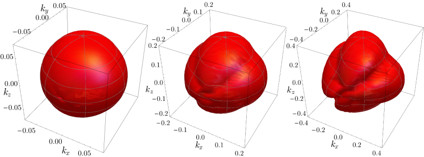
Figure 2: (Colors online) The red surfaces represent the orbit of a wave-vector $\mathbf{k}=(k_{x},0,0)$ under the action of the deformed rotations $\mathcal{R}={\mathcal{D}^{(f)}}^{-1}\circ R\circ\mathcal{D}^{(f)}$ where $f$ is the function defined in Eq. (28). Left: $k_{x}=0.07$. Middle: $k_{x}=0.2$ Right: $k_{x}=0.4$

In order to classify this group, we now observe that a map acting as in Eq. (20) transforms the four Pauli matrices linearly $\sigma^{\mu}\mapsto L^{\mu}_{\nu}\sigma^{\nu}$, and in turn this implies that $p^{(f^{\prime})}_{\mu}(k^{\prime})=L_{\mu}^{\nu}p^{(f)}_{\nu}(k)$. Moreover, the set of invertible linear transformations represented by $L_{\mu}^{\nu}$ must preserve the mass-shell $p^{(f)}_{\nu}p^{(f)\nu}=0$. By the Alexandrov-Zeeman theorem Zeeman (1964); Alexandrov (1967) this implies that the transformations $L_{\mu}^{\nu}$ must be a representation of the Lorentz group. Thus, a general change of inertial frame $(k^{\prime},a,M,\tilde{M})$ for the right-handed Weyl walks must be of the form

$$k^{\prime}(k)={\mathcal{D}^{(g)}}^{-1}\circ L_{\beta}\circ\mathcal{D}^{(f)},$$

$$M=\Lambda_{\beta},\quad\tilde{M}=\tilde{\Lambda}_{\beta},$$ (23)

where $L_{\beta}$, $\Lambda_{\beta}$ and $\tilde{\Lambda}_{\beta}$ are the $(\tfrac{1}{2},\tfrac{1}{2})$, $(0,\tfrac{1}{2})$ and $(\tfrac{1}{2},0)$ representations of the Lorentz group, respectively. The only difference in the case of left-handed Weyl walks is that the representations $\Lambda_{\beta}$ and $\tilde{\Lambda}_{\beta}$ are exchanged. Notice that

$$\mathcal{D}^{(f)}\circ{\mathcal{D}^{(g)}}^{-1}=M_{f}\circ n\circ n^{-1}\circ M_{g}^{-1}=M_{f}\circ M_{g}^{-1},$$ (24)

where

$$M_{f}(m)=f(n^{-1}(m))m$$ (25)

one has

$$\mathcal{D}^{(f)}\circ{\mathcal{D}^{(g)}}^{-1}(m)=h(m)m,$$ (26)

and thus

$$\begin{aligned} &({\mathcal{D}^{(g^{\prime})}}^{-1}\circ L_{\beta^{\prime}}\circ\mathcal{D}^{(f^{\prime})})\circ({\mathcal{D}^{(g)}}^{-1}\circ L_{\beta}\circ\mathcal{D}^{(f)})=\\ &({\mathcal{D}^{(g^{\prime})}}^{-1}\circ L_{\beta^{\prime}}\circ\mathcal{D}^{(f^{\prime})}\circ{\mathcal{D}^{(g)}}^{-1}\circ L_{\beta^{\prime}}^{-1})\circ L_{\beta^{\prime}}\circ L_{\beta}\circ\mathcal{D}^{(f)}=\\ &\mathcal{D}^{(g^{\prime\prime})}\circ L_{\beta^{\prime}\circ\beta}\circ\mathcal{D}^{(f)}\\ &\mathcal{D}^{(g^{\prime\prime})}:={\mathcal{D}^{(g^{\prime})}}^{-1}\circ L_{\beta^{\prime}}\circ\mathcal{D}^{(f^{\prime})}\circ{\mathcal{D}^{(g)}}^{-1}\circ L_{\beta^{\prime}}^{-1}\end{aligned}$$ (27)

It is then sufficient to prove that a function $f$ with the desired properties exists, otherwise the group of symmetries of the walk would be trivial. We have already shown in Section II.1 that the restriction $\mathbf{n}_{i}(\mathbf{k})$ of $\mathbf{n}(\mathbf{k})$ to $B_{i}$ define an analytic diffeomorphism between $B_{i}$ and the manifold $\mathsf{H}\subset\mathsf{U}$. Let us consider the solutions of Eq. (18), and define the function $g(\omega,r\mathbf{m}):=f(\omega,\mathbf{n}^{-1}(r\mathbf{m}))$, where $g$ is monotonic versus $r\geq 0$ for every $\mathbf{m}\in\mathsf{H}$. We notice that the function $g(\omega,r\mathbf{m})$ is well defined since $\mathsf{H}$ is star-shaped. Furthermore, if $g(\omega,r\mathbf{m})$ diverges on the boundary of $\mathsf{H}$, we have that the map $\mathcal{D}^{(f)}(k)$ defines a diffeomorphism between the set $C_{i}:=\{k=(\omega,\mathbf{k})|\mathbf{k}\in B_{i},\cos\omega=\lambda{\mathbf{k}}\}$ and the null mass shell $\mathsf{K}:=\{p\in\mathbb{R}^{4},\text{ s.t. }p^{\mu}p_{\mu}=0\}$. A possible choice of $f(k)$ which satisfies all the previous requirements is given by

$$\begin{aligned} &f(\omega,\mathbf{k}):=f^{\prime}(\bm{\mathrm{n}}(\mathbf{k})),\\ &\tilde{f^{\prime}}(r,\theta,\phi):=1+r\!\!\int_{0}^{r}\!\!\!\!ds\,\,\left(\frac{1}{a(s)}+\frac{1}{b(s,\theta,\phi)}\right),\\ &a(r):=1-r^{2},\quad b(r,\theta,\phi):=\cos^{2}2\phi+(\tfrac{1}{2}-r^{2}(1-\cos^{2}\theta\sin^{2}\phi))^{2}\end{aligned}$$ (28)

where we used spherical coordinates $n_{x}=r\cos\theta\cos\phi$, $n_{y}=r\sin\theta$, $n_{z}=r\cos\theta\sin\phi$ for the argument in the definition of the function $f^{\prime}:\mathsf{H}\to\mathbb{R}$, with the convention that for $\mathbf{n}=\mathbf{0}$ one has $\phi=0$.

In order to classify the most general transformation leaving the walk invariant, it is still possible to allow for transformations of the kind

$$k^{\prime}=\sum_{i}n_{j(i)}^{-1}n_{i},$$ (29)

$$a=0,\quad M=\tilde{M}=I,$$ (30)

where the region $B_{i}$ is mapped to the region $B_{j(i)}$. Notice that this corresponds to a permutation of the four regions $B_{i}$, which however must fulfil the constraint that $i$ and $j(i)$ must labe lregions corresponding to walks with the same chirality ($\{B_{0},B_{2}\}$ and $\{B_{3},B_{4}\}$). This part of the group thus corresponds to $\mathbb{Z}_{2}\times\mathbb{Z}_{2}$.

By considering the case $f=g$ in Eq. (23), we have

$$\mathcal{L}_{\beta}:={\mathcal{D}^{(f)}}^{-1}\circ L_{\beta}\circ{\mathcal{D}^{(f)}}$$ (31)

which is a non linear representation of the Lorentz group as the ones considered within the context of doubly special relativity Amelino-Camelia and Piran (2001); Amelino-Camelia (2002); Magueijo and Smolin (2003). It is easy to observe that, if $f^{\prime}(0)=1$ and $\partial_{\mu}f^{\prime}=0$ where $f(\omega,\mathbf{k})=f^{\prime}(\sin\omega,\mathbf{n}(\mathbf{k}))$ as in Eq. (28), the Jacobian $J_{\mathcal{L}_{\beta}}$ of $\mathcal{L}_{\beta}$ coincides with $L_{\beta}$. In the limit of small wave-vector we have that $\mathcal{L}_{\beta}=L_{\beta}+O(|\mathbf{k}|^{2})$ that is the non linear Lorentz transformations recover the usual linear one. In Fig. 2 we show the numerical evaluation of some wave-vector orbits under the subgroup of rotations of the nonlinear representation of the Lorentz group. We see how the distortion effects, which are negligible for small wave-vector, become evident at larger wave-vectors.

IV Conclusion

The analysis of the previous section can be in priniciple applied to any quantum walk dynamics for which we know a complete set of constant of motion. In particular we could consider the Dirac quantum walk of Ref. D’Ariano and Perinotti (2014), whose eigenvalue equation is $(p_{\mu}(\omega,k,m)\gamma^{\mu}-mI)\psi(\omega,k,m)=0$ where $\gamma_{\mu}$ are the Dirac $\gamma$ matrices in the chiral representation, $m$ is the particle mass and $p(\omega,k,m):=(\sin\omega,\sqrt{1-m^{2}}\mathbf{n}(\mathbf{k}))$. In this case we may generalize Definition 1 and allow for maps that change the value of $m$. We can then consider the invariance of the whole family of Dirac quantum walks parametrized by $m$. One could prove that the symmetry group of the Dirac walks include a non-linear representation of the De Sitter group $\mathbb{SO}(1,4)$.

Since the frequency (or energy) $\omega$ and the wave-vector (or momentum) $\mathbf{k}$ are the constant of motion of the quantum walk dynamics, the scenario we discussed so far deals with the changes of reference frame in the energy-momentum $(\omega,\mathbf{k})$ space. In particular we saw that the Lorentz group is recovered and one could wonder how to give a time-position description of the deformed relativity framework that we obtained in energy-momentum space. It is believed that the nonlinear deformations of the Lorentz group in momentum space have profound consequences on our notion of space-time. In particular we may have the emergence of relative locality Amelino-Camelia et al. (2011), i.e. the coincidence of events in space-time becomes observer dependent. This would imply that not only the coordinates on space-time are observer dependent, as in ordinary special relativity, but also that different observer may infer different space-time manifolds for the same dynamics. Non-commutative space-time and Hopf algebra symmetries Lukierski et al. (1991); Majid and Ruegg (1994); Kowalski-Glikman and Nowak (2002, 2003); Bisio et al. (2016c) have been also considered for a time-position space formulation of deformed relativity.

References

• Feynman (1982) R. Feynman, Int. J. Theor. Phys. 21, 467 (1982).
• Lloyd (2006) S. Lloyd, Programming the universe: a quantum computer scientist takes on the cosmos (Vintage Books, 2006).
• Hardy (2001) L. Hardy, quant-ph/0101012  (2001).
• Fuchs (2002) C. A. Fuchs, quant-ph/0205039  (2002).
• Chiribella et al. (2011) G. Chiribella, G. D’Ariano,  and P. Perinotti, Phys. Rev. A 84, 012311 (2011).
• Dakic and Brukner (2011) B. Dakic and C. Brukner, in Deep Beauty: Understanding the Quantum World through Mathematical Innovation, edited by H. Halvorson (Cambridge University Press, 2011) pp. 365–392.
• Khrennikov and Weihs (2012) A. Khrennikov and G. Weihs, Foundations of Physics 42, 721 (2012).
• Khrennikov et al. (2015) A. Khrennikov, H. d. Raedt, A. Plotnitsky,  and S. Polyakov, Foundations of Physics 45, 707 (2015).
• D’Ariano and Khrennikov (2016) G. M. D’Ariano and A. Khrennikov, Philosophical Transactions of the Royal Society of London A: Mathematical, Physical and Engineering Sciences 374 (2016), 10.1098/rsta.2015.0244http://rsta.royalsocietypublishing.org/content/374/2068/20150244.full.pdf .
• Schumacher and Werner (2004) B. Schumacher and R. Werner, quant-ph/0405174  (2004).
• Gross et al. (2012) D. Gross, V. Nesme, H. Vogts,  and R. Werner, Communications in Mathematical Physics , 1 (2012).
• Bialynicki-Birula (1994) I. Bialynicki-Birula, Physical Review D 49, 6920 (1994).
• Meyer (1996) D. Meyer, Journal of Statistical Physics 85, 551 (1996).
• Meyer (2001) D. A. Meyer, Journal of Physics A: Mathematical and General 34, 6981 (2001).
• Yepez (2006) J. Yepez, Quantum Information Processing 4, 471 (2006).
• Arrighi et al. (2014a) P. Arrighi, V. Nesme,  and M. Forets, Journal of Physics A 47, 465302 (2014a).
• Arnault and Debbasch (2016) P. Arnault and F. Debbasch, Physical Review A 93 (2016).
• Arrighi et al. (2014b) P. Arrighi, S. Facchini,  and M. Forets, New Journal of Physics 16, 093007 (2014b).
• Arnault et al. (2016) P. Arnault, G. Di Molfetta, M. Brachet,  and F. Debbasch, Phys. Rev. A 94, 012335 (2016).
• Snyder (1947) H. Snyder, Physical Review 71, 38 (1947).
• D’Ariano (2011) G. M. D’Ariano, Phys. Lett. A 376 (2011).
• D’Ariano and Perinotti (2014) G. M. D’Ariano and P. Perinotti, Phys. Rev. A 90, 062106 (2014).
• Bisio et al. (2015) A. Bisio, G. M. D’Ariano,  and A. Tosini, Annals of Physics 354, 244 (2015).
• Bisio et al. (2016a) A. Bisio, G. M. D’Ariano,  and P. Perinotti, Annals of Physics 368, 177 (2016a).
• Bisio et al. (2016b) A. Bisio, G. M. D’Ariano,  and P. Perinotti, Phys. Rev. A 94, 04210 (2016b).
• Amelino-Camelia and Piran (2001) G. Amelino-Camelia and T. Piran, Physical Review D 64, 036005 (2001).
• Magueijo and Smolin (2002) J. Magueijo and L. Smolin, Phys. Rev. Lett. 88, 190403 (2002).
• Amelino-Camelia et al. (2011) G. Amelino-Camelia, L. Freidel, J. Kowalski-Glikman,  and L. Smolin, Phys. Rev. D 84, 084010 (2011).
• Kempe (2003) J. Kempe, Contemporary Physics 44, 307 (2003)http://dx.doi.org/10.1080/00107151031000110776 .
• Ambainis et al. (2001) A. Ambainis, E. Bach, A. Nayak, A. Vishwanath,  and J. Watrous, in Proceedings of the thirty-third annual ACM symposium on Theory of computing (ACM, 2001) pp. 37–49.
• Susskind (1977) L. Susskind, Phys. Rev. D 16, 3031 (1977).
• Zeeman (1964) E. C. Zeeman, Journal of Mathematical Physics 5, 490 (1964).
• Alexandrov (1967) A. D. Alexandrov, Canadian Journal of Mathematics 19, 1119 (1967).
• Amelino-Camelia (2002) G. Amelino-Camelia, International Journal of Modern Physics D 11, 35 (2002).
• Magueijo and Smolin (2003) J. Magueijo and L. Smolin, Physical Review D 67, 044017 (2003).
• Lukierski et al. (1991) J. Lukierski, H. Ruegg, A. Nowicki,  and V. N. Tolstoy, Physics Letters B 264, 331 (1991).
• Majid and Ruegg (1994) S. Majid and H. Ruegg, Physics Letters B 334, 348 (1994).
• Kowalski-Glikman and Nowak (2002) J. Kowalski-Glikman and S. Nowak, Physics Letters B 539, 126 (2002).
• Kowalski-Glikman and Nowak (2003) J. Kowalski-Glikman and S. Nowak, International Journal of Modern Physics D 12, 299 (2003).
• Bisio et al. (2016c) A. Bisio, G. M. D’Ariano,  and P. Perinotti, Philosophical Transactions of the Royal Society of London A: Mathematical, Physical and Engineering Sciences 374 (2016c).