Spectroscopy of very hot plasma in non-flaring parts of a solar limb active region: spatial and temporal properties

Abstract

In this work we investigate the thermal structure of an off-limb active region in various non-flaring areas, as it provides key information on the way these structures are heated. In particular, we concentrate in the very hot component ($>3~{}\mathrm{MK}$) as it is a crucial element to discriminate between different heating mechanisms. We present an analysis using Fe and Ca emission lines from both SOHO/SUMER and HINODE/EIS. A dataset covering all ionization stages from Fe X to Fe XIX has been used for the thermal analysis (both DEM and EM). Ca XIV is used for the SUMER-EIS radiometric cross-calibration. We show how the very hot plasma is present and persistent almost everywhere in the core of the limb AR. The off-limb AR is clearly structured in Fe XVIII. Almost everywhere, the EM analysis reveals plasma at $10~{}\mathrm{MK}$ (visible in Fe XIX emission) which is down to $0.1\%$ of EM of the main $3~{}\mathrm{MK}$ plasma. We estimate the power law index of the hot tail of the EM to be between $-8.5$ and $-4.4$. However, we leave an open question on the possible existence of a small minor peak at around $10~{}\mathrm{MK}$. The absence in some part of the AR of Fe XIX and Fe XXIII lines (which fall into our spectral range) enables us to determine an upper limit on the EM at such temperatures. Our results include a new Ca XIV 943.59 Å  atomic model.

1 Introduction

Decades of observations have unveiled the difficult task of understanding how and where the energy is deposited for the creation and maintenance of the solar corona. Various physical mechanisms have been proposed (see Reale, 2014, for a review) which may dominate depending on the local environment. Active regions (AR) are the most visible manifestation of the enduring corona. These are the hottest part of the non flaring corona, with strong UV and X-ray emission. ARs are generally composed of coronal loops which are classed in two main thermal categories: the hot and low-lying loops (3MK), less dense than equilibrium conditions, which are concentrated in the core; the warm loops (1MK), larger and more dense than equilibrium conditions, which are located above the AR core (Reale, 2014). It is not yet clear if these different properties are the result of different physical processes at work or are the manifestation of the same process observed in a different evolutionary state.

In recent years new observational signatures of coronal heating have been identified, which we believe, if completely understood, could be essential to progressing our understanding of the corona: a small amount of very hot plasma ($>5~{}\mathrm{MK}$) has been detected in several quiescent ARs (see e.g. Reale (2014) for a review). This detection is important as it confirms a prediction made several years earlier from the the modeling of coronal loops heated impulsively over small (sub-resolution) scales (e.g. Parker, 1988; Cargill, 1994; Klimchuk, 2006, 2015). Such models predict at larger spatial scales (at the spatial resolution reached by the modern instruments) a multi-thermal plasma along the line of sight. The very hot plasma provides evidence of the transitory (short-lifetime) state of the cooling plasma in these loops. The importance of observing such small amounts of very hot plasma relies on the fact that it is unique to impulsive heating events. This is the signature, for an unresolved spatial scale, of thin loops (strands) each heated independently over a short time.

One of the various diagnostics techniques used to test coronal heating models is the sampling of the heating-cooling process in loops, which shows different observational signatures depending on the way the heating happens. The differential emission measure (DEM) distribution with the temperature samples this process and is a common way of investigating the heating of loops (Cargill, 2014). A typical AR DEM increases as a power law of the temperature up to a maximum around $3~{}\mathrm{MK}$, with an index which may change and probably depends on the level of magnetic flux. Typically $EM\sim T^{3-5}$ (Warren et al., 2012; Del Zanna et al., 2015b). This index constrains the frequency at which the energy is released in the form of heating. At temperatures above the peak, the DEM decreases drastically, but the difficulty of the measurements (mostly carried out with EUV data) makes it hard to define the shape of this distribution above about $5~{}\mathrm{MK}$. In most of the cases it can be fitted with a power law function, but simulations of nanoflares heating reveal that this is not always the case (Barnes et al., 2016). This high temperature component of the DEM is the signature of the first phase of cooling which, for this reason, possibly conserves more information on the heating process and the amount of energy deposited (e.g. Parenti et al., 2006). The existing EUV instruments have difficulty in detecting emission above about $5~{}\mathrm{MK}$ as there is very little plasma at these temperatures (Winebarger et al., 2012) and because only a few relatively weak UV spectral lines form at these temperatures. For these reasons the DEM is not well constrained at high temperatures. X-ray spectra are more suitable, see for instance results from SMM Del Zanna & Mason (2014) and references therein. The upper limits in the DEM/EM imposed by the the measured fluxes that we found in the literature using EUV spectra are given by Hinode/EIS Ca XVII, SOHO/SUMER Fe XVIII and SDO/AIA 94 channel (Fe XVIII). Estimations from these datasets of the power law index ($EM\sim T^{\alpha}$) change from -6 to about -14 (Warren et al. (2012) see Table 5). The sounding rocket EUNIS-13 (Brosius et al., 2014) enabled measurements of extended Fe XIX emission in an on-disk AR. Without the possibility of performing a full DEM analysis, they provided a Fe XII/Fe XIX EM ratio of about 0.59 in the AR core. This assesses the difference a relation between relatively cool coronal plasma ($1.5~{}\mathrm{MK}$) and much hotter plasma at about $10~{}\mathrm{MK}$.

In recent years observations of non-flaring ARs with X-ray instruments has intensified with the purpose of better constraining this slope (e.g. Miceli et al., 2012; Sylwester et al., 2010; Shestov et al., 2010). Additional constraints at high temperatures have been obtained combining EUV and Hinode/XRT soft-X ray emission (Golub et al., 2007) for an on disk AR (e.g. Reale et al., 2009b; Testa et al., 2011; Petralia et al., 2014). The results found were about two orders of magnitude variation of the EM from $3-10~{}\mathrm{MK}$. RHESSI, even though it is not sensitive to this faint plasma, has revealed its presence in the $6-10~{}\mathrm{MK}$ range (McTiernan, 2009; Reale et al., 2009a). Most recently, Hannah et al. (2016), using the NUSTAR hard X-ray telescope, found an even larger decrease of the EM by imposing upper limits on this quantity due the absence of observed emission at high temperature. Similarly, the FOXSI hard X-ray emission sounding rocket (Ishikawa et al., 2014) provided an upper limit to the DEM above $8~{}\mathrm{MK}$ for an on disk AR.

In this paper we address the issue of spatially and temporally characterizing the high temperature emission of a non-flaring active region with the aim of providing further constraints to the heating mechanism responsible for its formation and maintenance. Even though such plasma has been observed in several active regions, at present very little is known about the spatial and temporal distribution within the same active region. To our knowledge, this is the first time that the spatial distribution of this very hot component is given at different heights above the limb.

To minimize uncertainties in quantifying this plasma and its temperature, we used spectroscopic data from a single element (Fe). For the first time this type of analysis is carried out combining the SOHO/SUMER and Hinode/EIS spectra allowing the observation of iron lines in contiguous ionization stage from Fe X to Fe XIX to be used. This choice of instruments combination is at present unique: in provides a line sequence of a single element in a broad temperature range and lets our thermal analysis be independent of the plasma composition. We provide evidence of persistent emission from Fe XIX high in the corona, above the limb.

After presenting our observations in Section 2 and the data reduction in Section 3, we introduce the diagnostic technique in Section 4. Section 5 reports the results on the temporal analysis, Section 6 presents the inter calibration of the two instruments, while the results from the thermal analysis is given in Section 7. The conclusions are summarized in Section 8.

2 Observations

We ran HOP (Hinode Operation Plan) 211 on active region 11459 for several hours at the west limb between the 27 and 28 April 2012 using both the SOHO/SUMER (Wilhelm et al., 1995) and the Hinode/EIS (Culhane et al., 2007) spectrometers (Figure 1).

SUMER: After the loss of Detector A in 2006, due to failure of the readout electronics, only the B Detector remained available. In mid-2009, a degradation was observed in the center of the active area of the detector. As a protective measure, it was necessary to reduce the high voltage and the consequent reduction of the overall gain led to a drop of sensitivity in the central, KBr-coated, part of the photocathode, where it fell below detectable thresholds. Only the two uncoated (bare) areas of the detector (about 200 pixels each) were usable at the time of our observations. Additionally, since the resistivity of the microchannel plate (MCP) was observed to decrease with increasing temperature, to avoid a runaway effect, pauses were added in the observing sequences. All SUMER data sequences discussed here are made of sequences of 60 exposures of 75s each. After each pair of exposures a pause was added (of about 190s for the three sequences closest to the solar limb and of about 210s for the three sequences at a greater distance above the limb). Thus, each sequence can be thought as 30 regularly spaced pairs of 75s exposures.

SUMER observed in a sit-and-stare mode using the $\mathrm{1\arcsec\times 300\arcsec}$ slit for about eight hours (16:02:08 UT to 00:28:58UT on the 27th) centered at a solar distance of $992\arcsec$. In the following this will be called slit position 1. During this time SUMER scanned the wavelength range needed to cover the observation of Fe XVII, Fe XVIII (Ca XIV) and Fe XIX as listed in Table 1. As a result, each Fe line was observed for about two hours (60 exposures with 75 sec exposure time). An example of the spectra for these lines is shown in Figure 2.

A second sequence of observations, starting on the 28th at 00:35:55UT, was made by moving the pointing west of about $\mathrm{60\arcsec}$. After a first sequence which used the same slit, the slit was changed to $\mathrm{4\arcsec\times 300\arcsec}$ when scanning Fe XVII and XIX (in the following we call this outer slit position as position 2, see also Table 1).

EIS: EIS data consist of three rasters nominally pointed at the two SUMER slit center positions. Each raster was scanned in about two hours starting at 18:19:33 UT. The observing program used the $2\arcsec$ slit, which scanned eastward over 82 positions with 2″step and 90 seconds exposure time. The final field of view is $164\arcsec\times 376\arcsec$. Details of the observations are given in Table 1.

Our observations occured during the Hinode eclipse season, with the result that not all the common field of view of SUMER and EIS was exploitable. This is shown in Figure 1.

We point out that the data we used are not all co-temporal. For this study, we tried to select quiescent areas of the AR to minimize the temporal evolution of the plasma. However, this aspect has to be taken into account in the interpretation of our results. We discuss this aspect in Section 5.

Prior to and during our observations, AR 11459 flared a few times, with moderate intensity. These flaring events left some signatures on our datasets. Some small activity had already happened while observing with SUMER in slit position 1, while observing the Fe XVIII 1118.0575 Å. A hot loop system passed through the SUMER slit as shown in Figures 3 and 12. This was also imaged by the second raster of EIS. The first flare happened on the 27th of April with the peak at 21:04UT. A C2.2 flare followed in the same region peaking at 23:39UT while SUMER was observing Fe XVII 1153.16 Å  (Figure 3). On the 28th there was a C1.5 flare (peak at 0:43UT) and a C1.4 (peak at 1:54UT), but our data does not look to be affected. We discuss this in more detail in the following sections. In our analysis we also used the continuous monitoring provided by SDO/AIA for reference and comparison.

As the aim of this work is to investigate the quiescent conditions of ARs, the data affected by the flares were discarded from our analysis. Details of our data selection are given in the next Section.

Table 1: SUMER and EIS observations for 27/28th April 2012.

Inst.	start day, hour	end day, hour	Center	Main line	position n.
	[UT]	[UT]	[x″, y″]	[Å]
SUMER	27, 16:00:53	27, 18:47:11	[962, -271.9]	Fe XVIII 974.86,	1
				Ca  XIV 943.59
SUMER	27, 18:51:49	27, 21:38:05	[962, -271.9]	Fe XIX 1118.0575	1
SUMER	27, 21:42:39	28, 00:28:58	[962, -271.9]	Fe XVII 1153.1653	1
SUMER	28, 00:34:40	28, 03:29:55	[1025.5, -274.7]	Fe XVIII 974.86,	2
				Ca  XIV 943.59
SUMER	28, 03:34:57	28, 06:30:12	[1025.5, -274.7]	Fe XVII 1153.1653	2
SUMER	28, 06:35:07	28, 09:30:23	[1025.5, -274.7]	Fe XIX 1118.0575	2
EIS	27, 18:19:33	27, 20:24:49	[951.7, -300.5]	Ca  XIV 193.87	1
EIS	27, 20:24:55	27, 22:30:11	[951.7, -300.5]	Ca  XIV 193.87	1
EIS	27, 23:01:40	28, 01:06:56	[1012.7, -300.3]	Ca  XIV 193.87	2

Note. — The table lists the coordinates of the FOV center obtained with the co-alignement, as well as the high temperature lines observed.

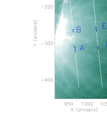
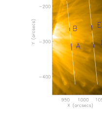
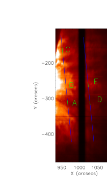
Figure 1: AIA 94 (left) and 171 (middle) images obtained by averaging two exposures taken between 03:06 and 03:10 UT on April 28. The SUMER slit in both positions 1 and 2 is marked by the white line. The masks selected for the analysis are also marked in color. Right: EIS raster image in Fe XII 192.39 Å  intensity which started at 23:01 UT on April 27. The SUMER slit and the masks are also marked in color. The EIS raster is affected by the spacecraft eclipse.

3 Data reduction

The SUMER data were decompressed, wavelength-reversed, corrected for dead-time losses, local-gain depression, flat-field, and image distortion induced by the readout electronics. All the above steps were performed by using the standard software provided in $SolarSoft$ (Freeland & Handy, 1998).

SUMER off-limb data may be affected by stray-light. We estimated this contribution in two ways (detailed in Appendix B). SUMER spectra are not wavelength calibrated. We performed this calibration (presented in Appendix C).

The EIS data were corrected for instrumental effects and calibrated applying the $eis\_prep.pro$ (version 29-Jan-2015) available on $SolarSoft$. The radiometric calibration has recently been further improved by Del Zanna (2013a) and Warren et al. (2014). For our analysis we used the Del Zanna (2013a) calibration, but a discussion of the influence on the results obtained using a different calibration is presented in Section 6.

Before performing the data analysis, we processed the data to take into account various issues that could affect results. These are presented below.

We started by carrying out a co-alignment of the fields of views of EIS and SUMER, which was done by using the SDO/AIA images for reference. This was done for two reasons: the SUMER slit follows the SOHO roll, which is not aligned North-South, and the EIS raster data has a temporal dependence. The task is not easy as we were dealing with off-limb data where the structuring and image contrast are less marked than on-disk. For the first SUMER slit position 1, we found that the best way to proceed to co-align SUMER-AIA was to use the flare data (SUMER Fe XVIII and AIA 94 channel). For the slit position 2 we used the pair SUMER Ca X 557.766 Å  with AIA 171, and SUMER Ca X 574.011 Å  with AIA 171. The two Ca lines are observed about two hours apart, but the result of these two alignments were similar within 2″. Details of this work are given in Appendix A and the results are listed in column four of Table 1.

It is known that EIS is not aligned with respect to AIA. We first used the $eis\_aia\_offset.pro$ IDL procedure available in the $SolarSoft$ database to correct our EIS data. However, we were not satisfied with our results and we decided to proceed with an independent manual co-alignment based on cross-correlation. We used the AIA 195 channel and EIS Fe XII 192.394 Å. The details of the method are given in Appendix A and the results are given in Table 1.

3.1 Spectral line selection

Table 2 gives the list of the observed spectral lines and their fluxes used in this work. To reduce the uncertainties in the results of the thermal analysis, we minimized the effect of the elements abundance, by selecting only lines from Fe ions. We have enough Fe ions to cover the temperature range $6<\log T<6.95$. In addition, as we shall show, we performed several tests to monitor the effects of elemental composition on our results. To this line list we added Si VII to constrain the DEM and EM at low temperatures and Ca XIV, which was used for the intercalibration EIS-SUMER (see Sec. 6). This is, in fact, the only ion which is present in both instruments whose lines are free from blends. Our results should not be affected by element abundance variations as the chosen ions are all from low First Ionization Potential elements. In addition, the Ca XIV is formed at a temperature similar to Fe  XV and Fe  XVI which were observed by EIS.

The EIS high temperature lines from ions above Ca XIV and Fe XVI were absent or unusable because they were too blended. We also tried to extract Ca XVII 192.853  Å  but with no success. To do this, we used the Ko et al. (2009) method, which deblends this line from the Fe  XI and O V lines. We used the theoretical CHIANTI ratio between the Fe  XI 188.1/192.8 to fix the Fe  XI 192.8  Å  profile parameters, but could not find any good solutions to the multi-line fitting. We then recalculated this ratio directly for the data by selecting a quiet off-disk area far from the limb, where the 192.8  Å  line was very symmetric, and did not show any evidence of the presence of O  V and Ca XVII. We then assumed that O  V and Ca XVII were absent. With this new ratio value we found the best solution of the multi-Gaussian fitting was one in which Ca XVII line was absent. We concluded that in our data, this line was absent or too faint to be measured. In conclusion, the high temperature plasma is only covered by the SUMER data. Our analysis was carried out over several masks as described in the following Sections. We used the $eis\_mask\_spectrum.pro$ to select the masks in the EIS rasters and $spec\_gauss\_eis.pro$ available in $SolarSoft$ to perform a multi-Gaussian fitting of the resulting spectra.

Amongst the hot lines in the SUMER spectra, the Fe  XVIII 974.860 Å  blend required particular attention (see Figure 2). This blend has previously been discussed by Teriaca et al. (2012) and is due to the presence of a ghost image (caused by the electronics) of the H  I 972.54 Å line falling about 2.8 Å  red-ward of this line, and Si  VIII 974.58 Å. The amplitude of the ghost has been estimated by these authors to be about 1/200 the main line and it cannot easily be fitted within the blend. Having the H  I 972.54 Å line in our spectra, we could estimate the ghost by adopting this value to correct our Fe line flux. We found its contribution to be only $1\%$ to $2\%$. The Fe  XVIII line was fitted using two Gaussians profiles in order to deblend it from the Si  VIII. However, the result for the different masks was not always satisfying. We then estimated the contribution of the Si  VIII by calculating the intensity ratio with the Si  VIII 1182.48 Å lines we had in the spectrum, which is well isolated and has similar amplitude. We estimated this ratio from our data by selecting a quiet region (mask $F$) where Fe  XIX is absent and we expected to have none or a very small contribution of Fe  XVIII to the blend. The result of the double Gaussian fit to the spectra of mask $F$ gives the Si  VIII 974.58/ 1182.48 Å = 1.04. This value is consistent with Feldman et al. (1997) off-limb observation who found a value 1 for this ratio, while Curdt et al. (2004) found a smaller value (0.7). We adopted our result to correct the Fe  XVIII in our masks. Considering that in the masks chosen for the thermal analysis the Fe  XVIII line is about 20 times brighter than the Si  VIII 1182.48 Å, our uncertainty on the blend remains within the assumed $20\%$ uncertainty of the fluxes.

We indeed assumed an error of $20\%$ in the lines flux. This value includes uncertainties in the atomic physics, ionization/recombination rates calculations (which, for certain ions could be larger). We are aware that other factors may arise to increase the uncertainty. For instance, the EIS calibration which will be discussed in Sec. 6. The lack of co-temporal data may also imply some inconsistency in the analysis. This will be discussed in Sec. 8.

Figure 2 shows an example of the hot lines in the SUMER spectra for mask $A$ together with the result of multi-Gaussian fitting.

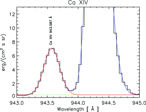
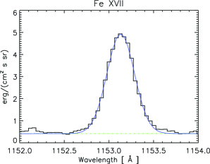
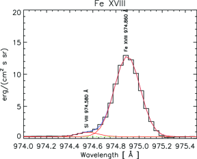
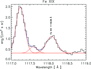
Figure 2: Spectra of mask $A$ for the SUMER hot lines and their resulting fit. The red curve marks the single Gaussian fit, while the blue curve is the sum.

3.2 Upper limit on the flux for Fe  XIX and Fe  XXIII

Above $3~{}\mathrm{MK}$ the non flaring plasma produces faint emission. To better constrain our thermal analysis we estimated an upper limit of the flux for those flaring lines falling in the spectral range of our data, but which were not visible. This is the case for SUMER Fe  XIX 1118.06 Å   in mask $B$ and for the EIS Fe  XXIII 263.77 Å  in the other masks.

Assuming a Poisson background statistics approximated by a Gaussian, we set a $3\sigma$ confidence level as the minimum threshold for detection of the line signal above the background photon counts. We selected a wavelength interval similar to the expected line width. We used this to calculate the minimum flux needed for the spectral line to be measurable. The results are given in Table 2.

Table 2: Lines list and total fluxes (I).

Ion	$\lambda$	log $T_{\rm max}$	I(A)	I(B)	I(C)	I(C)	I(D)	I(E)	Inst.
	[Å]	[K]			[18:19UT]	[20:24UT]
Si  VII	275.38	5.79	299.7	525.1	53.6	75.7	56	135.2	EIS
Fe  X(sbl)	257.26	6.04	1347.4	2189.9	526.3	674.8	586.3	988	EIS
Fe  XI	188.30	6.13	1258.0	1764.1	868.5	917.2	640.4	935.9	EIS
Fe  XII	192.39	6.20	953.5	1283.0	878.4	926.8	446.2	656.6	EIS
Fe  XIII	202.04	6.25	2824.1	3279.1	2999.9	3041.3	1504.6	2025.3	EIS
Fe  XIV	264.79	6.29	2264.3	2741.5	2532.4	2474.0	654.6	1038.07	EIS
Fe  XV	284.16	6.34	19078.8	21675.8	18155.5	17585	7848.5	10187.5	EIS
Fe  XVI	262.98	6.43	1474.1	1565.3	1154.9	946.7	384.0	517.7	EIS
Ca  XIV	193.87	6.57	112.1	92.3	63.8	45.5	28.6	32.8	EIS
Ca  XIV	943.59	6.56	4.0	3.79	2.72	2.72	1.44	1.76	SUMER
Fe  XVII	1153.16	6.73	3.4	2.7	1.82	1.82	0.97	1.6	SUMER
Fe  XVIII	974.86	6.86	6.5	4.8	3.18	3.18	2.17	2.77	SUMER
Fe  XIX	1118.06	6.95	0.5	$<$ 0.11	0.76	0.76	0.22	0.22	SUMER
Fe  XXIII	263.765	7.16	$<$3		$<$3	$<$3	$<$3	$<$3	EIS

Note. — SUMER and EIS lines list and total fluxes (I) for each mask (from $A$ to $E$) used for the analysis of Sec. 7. The fluxes are in [$erg/cm^{2}/s/sr$]. The theoretical position of the line and the temperature of maximum formation are given in columns two and three. ($<$ ): upper limit imposed as the line is not visible; (sbl): self-blended line.

4 Plasma diagnostics methods

We summarise the plasma diagnostics that are used in this work, while further details can be found in Parenti (2015).

For the EUV-UV optically thin lines the total intensity is given by

$$I(\lambda)=\frac{1}{4\pi}\int_{l}{Ab~{}G(T_{e},n_{e})~{}n_{e}n_{H}dl}$$ (1)

where $l$ is the line of sight through the emitting plasma, $Ab$ is the abundance of the element with respect to hydrogen, $G(T_{e},n_{e})$ is the $contribution~{}function$ which contains all the atomic physics parameters, $n_{e}$ and $T_{e}$ are the electron number density and temperature and $n_{H}$ is the hydrogen number density.

For the thermal analysis we need to know the electron density distribution in the AR. One method of estimating the electron density is given by calculating the ratio of two line intensities from the same ion, where at least one involves a metastable level $m$. This make the ratio density dependent, assuming the temperature of the maximum of the ionization fraction of the ion. The density is then inferred by matching the ratio derived from observations with the theoretical value calculated at different densities. The results of this analysis are presented in App. D.

To estimate the distribution of the plasma emission measure with the temperature, there are various methods which differ in the approximations applied. We introduce the column emission measure (EM, Ivanov-Kholodnyi & Nikol’Skii, 1963; Pottasch, 1963) along the line of sight $l$, as

$$EM=\int_{l}n_{e}n_{H}dl$$ (2)

If we assume that the emitting plasma along $l$ is isothermal at $T_{c}$ and the electron density known ($n_{c}$), using Eq. 1 we can write

$$EM(T_{c})=\frac{4\pi I(\lambda)}{G(T_{c},n_{c})}$$ (3)

If the density is unknown, a first approximation test on the temperature distribution of the plasma is given by plotting EM($T_{e}$) as function of $T_{e}$, for a set of lines formed in a wide range of temperatures. This is called the emission measure loci approach. A necessary condition for the plasma to be isothermal is that these curves cross at the plasma temperature. However, this plot gives only an indication of the plasma distribution as the uncertainties on the measures and data inversion can introduce additional solutions to the inversion (Guennou et al., 2012).

When a set of lines from optically thin plasma formed at different temperatures is available, the differential emission measure (DEM) inversion is more appropriate to probe the multi-thermal plasma. The DEM is proportional to $n_{e}n_{H}$ (variable with $T_{e}$) in the temperature intervals $dT_{e}$ and it is defined here as

$$\mbox{\it DEM}(T_{e})=n_{e}n_{H}\frac{dl}{dT_{e}}$$ (4)

We also introduce the effective temperature, which is the DEM-weighted average:

$$T_{eff}=\frac{\int DEM(T)\times TdT}{\int DEM(T)dT}.$$ (5)

The thermal analysis using these diagnostics is presented in Sec. 7.

For the diagnostic analysis in this work we used the CHIANTI v.8 atomic database and software (Dere et al., 1997; Del Zanna et al., 2015a) to calculate the theoretical emissivities of the spectral lines. A particular case was the treatment of Ca XIV 943.59  Å, which will be discussed in Sec 6.

We adopted the CHIANTI default ionization equilibrium, and Feldman (1992) elemental abundances. This latter choice was made after several tests we did changing element composition in the EM loci approach and DEM inversions. Even if the effect of composition on the result is small, we found Feldman (1992) data to produce the better observed versus theoretical fluxes ratio. We adopted a density of $10^{9}~{}\mathrm{cm^{-3}}$ for the SUMER slit in position 1 and $4\times 10^{8}~{}\mathrm{cm^{-3}}$ for position 2 derived from the analysis presented in Appendix D.

5 Temporal variability and sub-data selection

We first made an investigation of the spatial and temporal properties of the AR along the SUMER slit in the hot lines. This has been useful to the selection of the region of interest for detailed investigation. We mostly used SUMER data, where the signal is strong.

5.1 Spatial structuring and temporal variability in hot lines

Figure 3 shows the intensity of the SUMER Fe XVII – XIX lines along the slit and for the sixty exposures on April the 27th, slit position $1$. From the top to the bottom, they have been ordered following the time sequence of data acquisition. The plots have been saturated to highlight the fainter structuring of the AR, and the brightest regions in yellow correspond to the flaring areas (around $Y=-230\arcsec$).

The Fe XVIII sequence shows a very bright area corresponding to the passage of a hot loop accross the slit (this is the one used to co-align SUMER and EIS, see also Figure 12 which is plotted using a different contrast). At both its sides of the hot loop we can identify faint structures whose flux seems to remain almost constant in time. This suggests that they are not affected much by the flare. We highlight them in the Figure 3 by pairs of vertical lines (see also Table 3, masks $A$ and $C$). In line with our aim of investigating non-flaring regions, we selected these two area as candidates to pursue our analysis. We also added a third region which was taken as a sample of the unstructured emission (mask $B$), which appears faint in all the plots of Figure 3. The details of these masks are listed in Table 3. Some structuring is still visible in the AR core.

A similar analysis has been carried out for the SUMER slit position 2 and is reported in Annex E. Here we identified two other candidate regions for the thermal analysis.

The structuring of the AR in hot lines has been extracted by temporally averaging the exposures. Reducing the background noise thus makes it easier to see the fainter regions (section 5.1.1). We also carried out a temporal analysis of these regions to understand better how much their flux varies with the flaring activity (section 5.1.2).

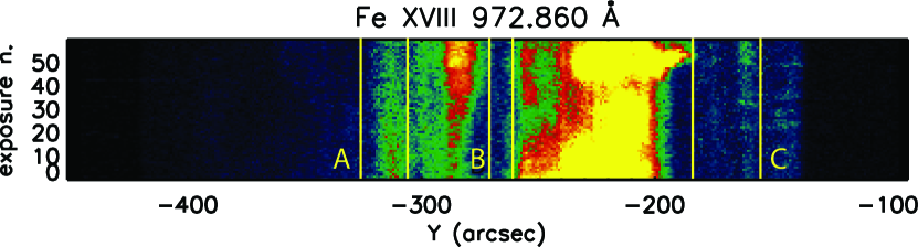
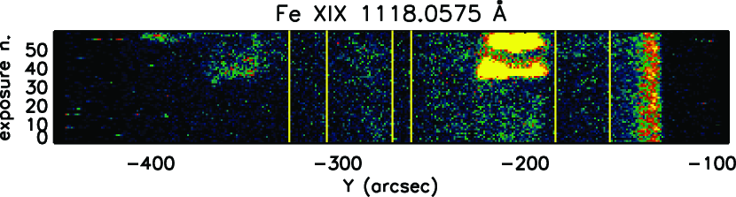
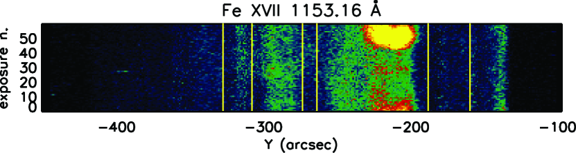
Figure 3: SUMER Fe XVII, Fe XVIII and XIX intensities along the slit in position 1, plotted for the sixty exposures (with 75 seconds exposure time). The images have been saturated to enhance the fainter emission at the side of the flare. The colour range represents, from top to bottom, 0-99, 0-10, 0-40 counts/pixel. The three vertical pairs of yellow lines mark the three masks $A$, $B$ and $C$. The limb is on the right side of the plots.

5.1.1 Spatial structuring

Figure 4 top shows the integrated intensity of the Fe XVIII line profile for the spectra averaged over the sixty exposures, plotted along the SUMER slit in position 1 using one pixel spatial resolution. The north is on the right of the plot. This figure shows well the structuring of the AR. As in Figure 3, the data in the range approximately Y= [-260″, -190″] are due to the hot loop, while the vertical pairs of dashed lines mark the three areas (masks) selected for the analysis.

Figure 4 bottom shows the same integrated intensities for the SUMER Fe XVII, Fe XIX and Ca X. The latter is used to represent the $1\mathrm{MK}$ corona. The three Fe lines are observed in three different spectral windows, which means that they are not co-temporal (only Ca X is co-temporal to Fe XVII). Nontheless, the intense Fe XVII and Fe XVIII lines have a similar pattern along the slit, which highlights brighter structures and fainter areas. On the other hand, the Fe XIX intensity outside the flaring region is very weak and there is little we can say using the intensity of a single pixel. In order to be able to use this line, for each of the selected regions we have spatially averaged the spectra. The three regions are marked by the pairs of vertical dashed lines. Going from the bottom of the slit towards the top, we find mask $A$: this is one of the faintest and most persistent structures in Fe XVII and Fe XVIII. Mask $B$ is located close to the slit centre and outlines a weak area between two bright ones. Mask $C$ is the closest to the limb and contains weak structuring.

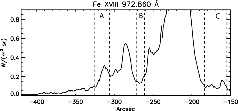
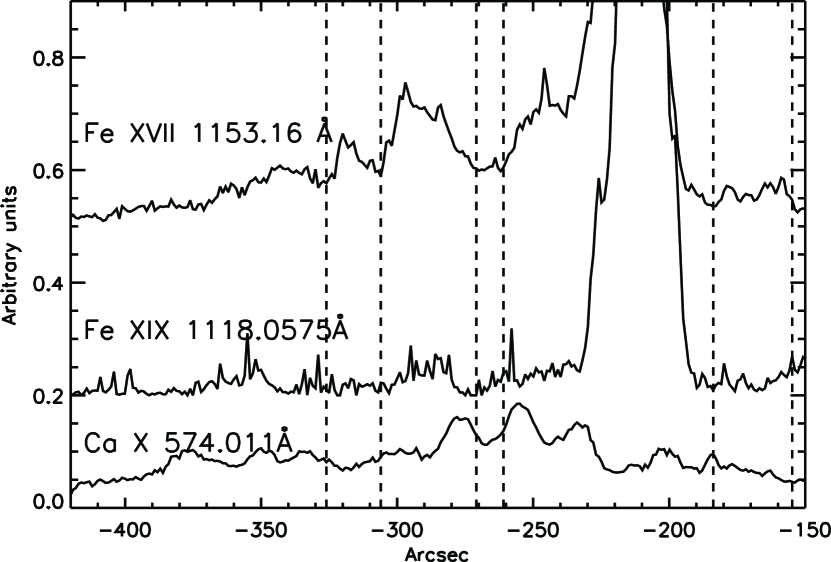
Figure 4: Top: SUMER Fe XVIII intensity along the slit integrated over the sixty exposures. The pairs of vertical dashed lines mark the three areas selected for further analysis. Bottom: same as the top plot for Fe XVII, Fe XIX and Ca X.

Table 3: The masks along the SUMER slit selected for the analysis.

Mask	Date	$Y1\arcsec<Y<Y2\arcsec$	$R_{\sun}\arcsec$
A	2012-04-27	-326, - 306	1007
B	2012-04-27	- 271, - 261	997
C	2012-04-27	-181.8, -154.8	958
D	2012-04-28	-320.5, -310.5	1075
E	2012-04-28	-268.8, -254	1052
F	2012-04-28	-421.2, -401.5	1117.7
G	2012-04-28	-421.2, -352.5	1076

Note. — The last two masks are used to test blends (see Sec. 3.1) and perform the SUMER wavelength calibration (described in Appendix C).

5.1.2 Temporal variability of the selected regions

To further investigate the temporal variability within the selected regions, we spatially averaged the spectra and kept some temporal resolution by averaging the spectra over only five exposures (six for Fe XIX). For example, Figure 5 shows the resulting light curves for mask $A$ and mask $B$. We compared these to light curves of the AIA 94 channel for the same masks using data integrated over 10 mins. The intensity has been corrected for the cooler component contributing to AIA 94 has estimated using the 171 channel, as described in Reale et al. (2011). For mask $A$, the hot component of AIA 94 is almost stable up to the time of the first flare at about 21UT ($\sim$ 420 mins in the plot). This component is mostly comparable to the SUMER Fe XVIII which, however, shows more variability. This line is blended with the Si VIII 974.58  Å  which has been removed. However the signal in a single point is weak and it is possible that some residuals of the Si line has affected the light curve. Some temporal variability is also visible in the Fe XIX which increases during the observations, while Fe XVII seems to be only marginally affected by the flare. We decided to keep this mask for our analysis and average out the temporal variability by using an average spectrum.

Also mask $B$ shows some variability, even though Fe XIX is always absent. This mask is closer to the flaring activity which is clearly visible in the AIA 94 curve. For this mask a signature is also visible in Fe XVII showing a peak delayed with respect to the AIA one. We used this mask by discarding the exposures of Fe XVII which were affected by the flare.

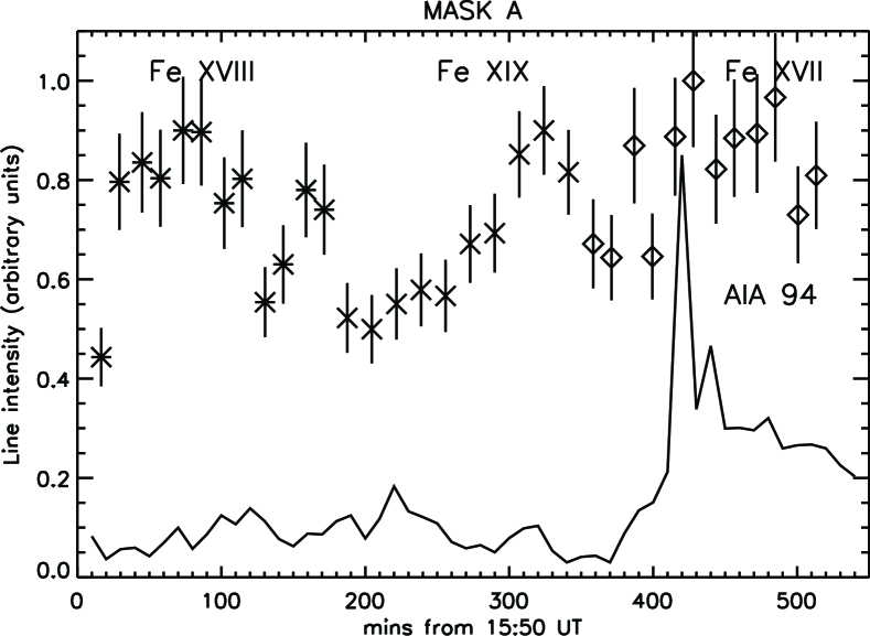
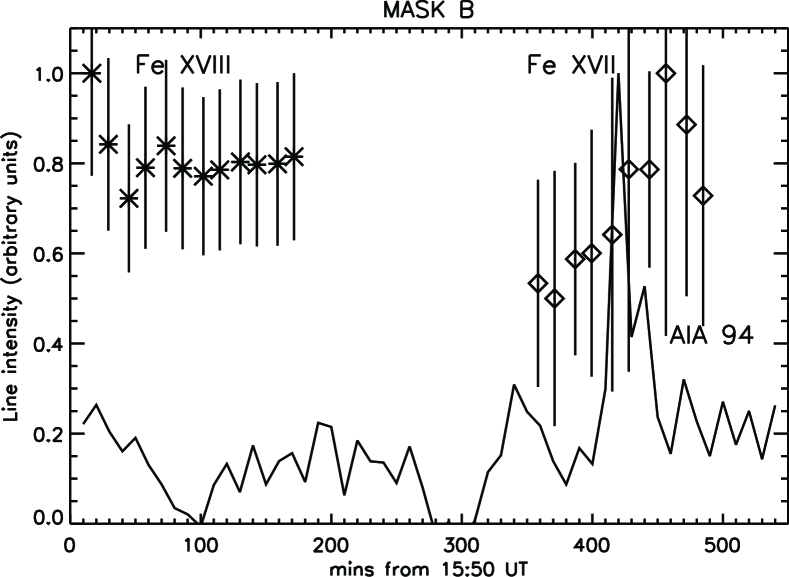
Figure 5: Light curves for the SUMER hot lines for mask $A$ and $B$ for slit position 1 compared to the AIA 94 corrected with the 171 channel. The fluxes from the three SUMER lines have been plotted using a different symbols. The error bars are from the line profile fitting accuracy.

In conclusion, this analysis shows that there is some variability in time of the hot lines, but only in one case can we see a clear link to the flaring activity. We discarded the affected exposures. To average out the temporal variability and increase the signal to noise of the data, we pursued the analysis on these masks by averaging the spectra over all the exposures, as shown in Figure 4 and 17. From these figures we see that the selected structures (apart from mask $E$), stay stable during the whole period of the observations (that is the time delay between observing Fe XVII and Fe XVIII).

6 SUMER-EIS cross calibration

The analysis carried out using integrated fluxes derived from different instruments could introduce inconsistencies due to the absolute radiometric calibrations. We carried out tests using the EM loci method on the Ca and Fe lines and found several issues that we had to solve. We used the data from some of the selected masks to address the problem.

6.1 Consistency in the EIS data

In addition to the pre-flight analysis (Lang et al., 2006), the absolute radiometric calibration of EIS has been investigated post-launch by Del Zanna (2013a), GDZ, and Warren et al. (2014), NRL. These last two introduce a different correction factor to the pre-flight calibration which, for the period of our observations, can reach a factor of 2.4 (see Figure 18 and Warren et al. (2014)). These differences have to be taken into account in the analysis of the data. All three calibrations are available in the $SolarSoft$.

Figure 6 shows the EM loci for the EIS data of mask $A$. There is consistency between the two results (GDZ and NRL), even though the use of the GDZ calibration results in larger EMs than in the NRL case, with a slightly lower peak temperature. In the following analysis we have used the GDZ calibration.

Figure 6: EIS EM loci for mask $A$ using both GDZ (dashed curves) and NRL (solid curves) calibrations.

6.2 Consistency in the SUMER data

Figure 7 shows the EM loci for the SUMER data for mask $A$, obtained by using the lines having a formation temperature close to the peak of the emission measure. From this set, only the high temperature lines will be retained for the thermal analysis presented in Section 7.

The EM peak is around $\log T=6.4$, which is typical of ARs. Also we note that the Ca  XIV loci plotted with the solid curved (CHIANTI v.8) is inconsistent with the rest of the curves, being it too high. Having investigated the problem, we found this to be an atomic data issue rather then a wrong choice of element abundances: the CHIANTI v.8 emissivity is not consistent with the observed one.
The Ca XIV forbidden line observed by SUMER at 943.58 Å is the strongest line within the ground configuration of this ion, between the ground state 2s² 2p^{3 4}S^3/2 and the first excited level, the 2s² 2p^{3 2}D^3/2. The excitation data in CHIANTI v.8 are from Landi & Bhatia (2005), and were calculated with the distorted wave (DW) approximation. It is well known that this approximation works very well for strong dipole-allowed transition, but typically underestimates the electron excitation rates of the forbidden lines, especially within the ground configuration. This was confirmed by a recent $R$-matrix calculation by Dong et al. (2012), where significant increases in several transitions rates were reported. The excitation rate for the 943.58 Å forbidden transition is about a factor of two higher with the Dong et al. calculations. We have taken the Dong et al. excitation rates and built a new CHIANTI model ion to be used for the present analysis. We supplemented these data with A-values from the recent calculations by Wang et al. (2016). The ratio with the strongest line, the resonance EUV line at 193.87 Å observed with Hinode EIS, is slightly temperature sensitive, but does not vary much with electron density. At log $T$[K]=6.4, the ratio between these two lines is a factor of 1.73 higher with the new model ion, which is significant.

The loci obtained with this new model is plotted as a dashed line in Figure 7, where it has become consistent with the ensemble of the curves.

Figure 7: EM loci for mask $A$ using SUMER data. The plot shows the change in the EM of Ca  XIV using the new calculation (dashed curve).

6.3 Combining EIS and SUMER data

When we plotted the EM locis from the two instruments together for the different masks, we found a systematic difference: at similar temperatures the SUMER emission measures were lower than the EIS ones. For instance, this is the case for two lines from Ca  XIV. We assumed this discrepancy was due to the SUMER degradation, discussed by Teriaca et al. (2012). We then made tests to calculate a correction factor to be applied to the SUMER fluxes. The correction factor can be obtained using data from an isothermal plasma, by comparing the measured to the theoretical lines ratio predicted by the CHIANTI database at the given temperature.

While a detailed discussion on the EM loci analysis will be given in the next section, here we just mention that the curves from the selected masks are all similar around the peak located between $\log T=6.4-6.5$. For our lines ratio analysis we selected the temperature obtained in mask $B$, as it is the one where the Fe  XIX is absent. This means that most of the Ca line emission is formed close to the EM peak temperature. Assuming this plasma temperature, we obtained a SUMER correction factor 1.8 using the GDZ EIS calibration (that is consistent with the expected degradation of the instrument performances estimated by Teriaca et al. (2012)). We also carried out the same analysis using the NRL EIS calibration and found a factor 1.4. For the following thermal analysis we used the GDZ factor.

7 Thermal analysis

This section presents the results from the thermal analysis using different DEM and EM methods.

7.1 EM Loci

Figure 8: E

M loci for the three masks of SUMER slit position 1 (first and second lines) and the two for SUMER slit position 2 (bottom line). The SUMER fluxes have been multiplied by 1.8. The two plots for mask $C$ are obtained using the data from the two EIS rasters with the same coordinates.

Figure 8 shows the combined EIS and corrected SUMER loci EMs for the selected masks for, SUMER slit position 1 (top and middle lines) and 2 (bottom line).

As already pointed out, there are similarities between these plots which all show the bulk of plasma at about $3~{}\mathrm{MK}$; which is a well known result (e.i. Parenti et al. (2010)). Additionally, the decrease of the EM is noticeable with the increase in solar height. The difference between them is mainly found in the absence of Fe  XIX for mask $B$ (in the figure we plotted an upper limit used for the DEM analysis). The cooler emission for this region might be representative of background AR plasma.

This first analysis suggests a new result: from above the limb to about $91~{}\mathrm{Mm}$ and over about $1.5\times 10^{2}~{}\mathrm{Mm}$ across the AR, the thermal properties above $3~{}\mathrm{MK}$ are similar almost everywhere.

For the region covered by the mask $C$ we can also provide temporal information, because this is the only mask that could be applied to both EIS rasters in position 1. The EM loci plots for this mask are shown in the middle row of Figure 8. Only the EIS curves can show differences (for both masks we used the same SUMER data). We see no significant change, so we conclude that the EM loci plots do not show evidence of spatial and temporal variations.

7.2 Differential emission measure

The DEM vs T curves (see Eq. 4) have been obtained with a method based on a simple chi-square minimization. We essentially used a modified version of the xrt_dem_iterative2.pro DEM inversion routine (Weber et al., 2004) in order to have more flexibility in the choice of input parameters. The standard routine, widely used in solar physics and available within $SolarSoft$, is based on the robust chi-square fitting routine (mpfit.pro). The DEM is modelled assuming a spline, with a fixed selection of the nodes. Since it turns out that the DEM solutions are quite sensitive to the choice of nodes, we modified the program to allow for the definition of the number and location of the spline nodes. We also introduced the option to input minimum and maximum limits to the DEM spline values, which are passed to (mpfit.pro). This was found to be particularly useful for constraining the upper limits of the highest temperature values. We used upper limits for the DEM values which provide radiances in the Fe XIX and Fe XXIII lines as given in Sec. 3.2.

Figure 9 shows the results from this inversion. The top plot shows the resulting DEM for mask $A$, overplotted with the points at the temperature of the maximum of the G(T), which represent the theoretical vs. the observed intensity ratio multiplied by the DEM value. The bottom plot contains all the masks together.

The temperature range for the inversion has been set to log $T$[K]=5.6 – 7.2. For all the DEM inversions we selected spline nodes at log $T$[K]= 5.6, 5.8, 5.95, 6.2, 6.35, 6.45, 6.55, 6.8, 7.2, which provide relatively good agreement (within 20–30%) between predicted and observed intensities, as shown in Table 4. The resulting DEM values are relatively smooth. Adding a few extra spline nodes in the 1–3 MK range can improve the agreement between observed and predicted intensities, but the DEM would be less smooth (as found for instance by Landi & Feldman (2008)).

Consistency was found between these results and the EM loci approach, the DEM curves are similar for all the masks. As expected, there is a decrease in amplitude of the DEM with an increase in the solar height. Some differences are found, but only at high temperatures.

The $1-2.5~{}\mathrm{MK}$ corona is represented by a double-peaked DEM. The hotter peak is at around $2.5~{}\mathrm{MK}$ and it is higher that the cooler peak for mask $A$, $C$ and $E$. The $3~{}\mathrm{MK}$ peak of the DEM of the off-limb corona is already known in literature (Reale, 2014). What is most interesting is the plateau above $5~{}\mathrm{MK}$ due to the observation of the high temperature lines. The DEM values at the main peak are so high that the effective temperature of emission for lines such as Fe  XVII and Fe  XVIII is about $3~{}\mathrm{MK}$, i.e. these lines are mainly formed far away from their peak formation temperatures (5 and $7~{}\mathrm{MK}$ respectively using the CHIANTI v.8 charge state distributions in ionization equilibrium). This issue is quite typical for active regions, as described e.g. in Del Zanna (2013b) and Del Zanna & Mason (2014). The peak at $2.5~{}\mathrm{MK}$ is very well constrained by the Fe  XVI and Ca  XIV lines. The fact that the DEM values around 3 MK are sufficient to explain the intensity of the Fe  XVII and Fe  XVIII lines means that the DEM above $3~{}\mathrm{MK}$ has to drop significantly by several orders of magnitude. However, whenever the Fe  XIX line is observed, its intensity requires a plateau in the DEM.

A further constrain at higher temperatures comes from the fact that the EIS Fe  XXIII 263.75 Å is not observed (we note that weak unidentified lines are present in active region EIS spectra, close to this line). We measured the variation of the EIS background near the line to estimate a 3 $\sigma$ value for the intensity of this line, as described in Sec. 3.2. We put an upper limit at log $T$[K]= 7.2 accordingly (the reason why the DEM increases slightly above $10~{}\mathrm{MK}$). From Table 4 we see that we have been quite conservative in choosing 3 $\sigma$, as the flux ratios between theoretical and measured values are well below 1.

The $10~{}\mathrm{MK}$ DEM is about $10^{3}$ times smaller than the $2.5~{}\mathrm{MK}$ peak, and even less for the cooler mask $B$ (here the Fe  XIX is not visible). This presence of very hot plasma has already been identified in some areas of ARs. Here we are able to extend our knowledge: this very hot plasma seems to be in all locations where we have a structured AR, with emission in the Fe  XVIII line, and it appears also to be persistent with time (at least within our observation time). In fact, the bottom of Figure 9 tells us that there is a temporal variation of the DEM above the $3~{}\mathrm{MK}$ between masks $C1$ and $C2$. This is the area very close to the limb and probably subjected to more AR variability. However, the $10~{}\mathrm{MK}$ DEM is not affected.

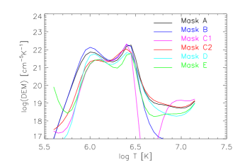
Figure 9: Top: Results from the DEM inversion for position 1 on mask $A$. The points are plotted at the temperature of the maximum of the G(T), at the theoretical vs. the observed intensity ratio multiplied by the DEM value. Bottom: The DEM for all the masks analyzed in this work.

7.3 Emission measure

Figure 10 top-left shows the emission measure (solid-blue line) for mask $A$ obtained by integrating the DEM of Figure 9 over a temperature bin of size 0.2 (in logarithm scale). In the Figure we also overplotted the EM resulting from 200 inversions by the DEM code, by randomly varying each flux within $20\%$. These are shown as a light gray cloud of solutions within each temperature bin. The bin size $d\log T=0.2$ is a good compromise to maximize the temperature resolution and to minimize the spread of the solutions within each temperature bin. The degradation of the solution with a smaller temperature bin is illustrated by the bottom-right plot of this figure.

We compared this calculation with the EM derived applying a different method. We used the Monte Carlo Markov Chain (MCMC) differential emission measure algorithm distributed with the $PINTofALE$ (Kashyap & Drake, 1998, 2000; Drake & Kashyap, 2010) spectral analysis package testing different input parameters.

With respect to several other methods, the MCMC method has the advantage of not imposing a predetermined functional form for the solution, and, most importantly, it provides confidence limits on the most probable DEM, thus allowing a determination of the significance of apparent structures that may be found in a typical reconstruction. The algorithm assumes that the uncertainties in the intensities are uncorrelated so that systematic errors in the calibration, which could depend on the wavelength, or in the atomic data, which could vary by ion, are not accounted for. The code has been set to perform 200 explorations (batches) of the parameter space, and 200 Monte Carlo realizations for each exploration. Figure 10 top-right shows the resulting EM from this method applying the same parameters of the left plot. In a similar way, Figure 11 shows the MCMC EM for mask $B$ (red line) with the cloud of solutions. The EM obtained from the DEM applying the chi-square minimization method (presented in Sec. 7.2) is overplotted in blue.

As seen in Sec. 7.2, the plasma distribution is dominated by a main peak around $3\mathrm{MK}$, followed by a drastic drop of the EM at high temperature. Overall, in the interval $6.5<\log T<7$ the EM looks to drop more (by about one order of magnitude) in mask $B$ than in mask $A$.

When we compare the solutions for one mask for the two methods, we see that they are consistent in most temperature bins. More discrepancies are found at low temperature, where the inversion is less constrained, and for the $\log T=6.8$ bin. In general the high temperature tail drops more rapidly with the first method.

As mentioned, to better constrain the solutions we decided to adopt a binsize of $\log T=0.2$, as a smaller one produces solutions with greater dispersion in each temperature bin. This is shown for instance for mask $A$ in Figure 10 bottom right. We checked the effect of extending the temperature range to higher values for those masks where the Fe  XXIII was used as upper limit. This is a flare line whose temperature of formation extends beyond $10~{}~{}\mathrm{MK}$. This inversion is shown for mask $A$ in Figure 10 bottom left. We see again that at high temperature the solutions in each bin spans a larger interval.

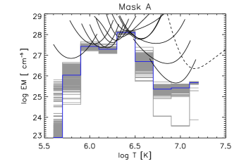
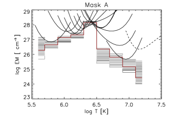
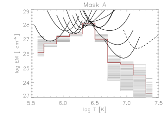
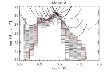
Figure 10: Mask $A$ EM loci. Top-left: in blue the EM derived from Sec. 7.2. Overplotted are the results from 200 runs varying the lines flux (see text). The EM loci are overplotted. The loci of the upper limit Fe  XXIII line is plotted with the dashed line. Top-right: results from the MCMC inversion (red) with their clouds of solutions using the same parameters than the left plot (a temperature binsize set to 0.2 and the maximum temperature to $\log T=7.2$). Bottom-left: result by extending the temperature range to $\log T=7.4$; Bottom-right: result by assuming a binsize of $\log T=0.1$ and maximum temperature of $\log T=7.2$.

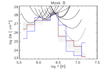
Figure 11: Result from the MCMC inversion (red line) for mask $B$ with the cloud of solutions, assuming the temperature binsize of 0.2 and the maximum temperature to $\log T=7.2$. The EM integrated from the DEM of Figure 9 for the same mask is plotted with the blue line. The loci EM are overplotted. The loci of the upper limit line is plotted with the dashed line.

Table 4: Ratios (R) of predicted vs. observed radiances of the selected lines for the various regions.

Ion	$\lambda$[Å]	log $T_{\rm eff}$[K]	R(A)	R(B)	R(C1)	R(C2)	R(E)	I(D)
Si  VII	275.38	6.00	1.01 (1.16)	1.02 (1.15)	1.06	1.02	1.06	1.03
Fe  X (sbl)	257.26	6.05	0.90 (0.54)	0.88 (0.52)	0.94	0.75	0.77	0.85
Fe  XI	188.30	6.12	1.17 (0.89)	1.19 (0.91)	1.09	1.0	1.12	1.17
Fe  XII	192.39	6.23	1.05 (1.13)	1.02 (1.12)	1.06	1.0	1.15	1.09
Fe  XIII	202.04	6.33	0.74 (0.89)	0.81 (0.92)	0.78	0.76	0.58	0.64
Fe  XIV	264.79	6.37	1.03 (1.21)	1.04 (1.10)	0.99	0.91	1.26	1.21
Fe  XV	284.16	6.40	1.25 (1.54)	1.23 (1.45)	1.26	1.06	0.99	1.07
Fe  XVI	262.98	6.42	0.84 (0.91)	0.80 (0.90)	0.84	0.84	1.04	1.0
Ca  XIV	193.87	6.45	0.86 (0.62)	0.91 (0.78)	0.84	1.11	1.04	1.14
Ca  XIV	943.59	6.45	1.04 (0.80)	0.97 (0.87)	0.87	0.81	0.91	0.93
Fe  XVII	1153.16	6.46	0.84 (0.66)	0.91 (0.82)	0.88	0.83	0.91	0.70
Fe  XVIII	974.86	6.50	1.16 (0.87)	1.14 (0.86)	1.17	1.32	1.07	1.09
Fe  XIX	1118.06	6.97	0.97 (1.03)	0.54 (0.98)$\ast$	0.91	0.66	0.97	0.97
Fe  XXIII$\ast$	263.765	6.95	0.15 (0.02)	-	0.25	0.16	0.1	0.1

Note. — In the first two columns we list the dominant contribution to the observed spectral lines. Note that the Fe  X 257.26 Å is a self-blend of two transitions. As an indication of where the lines mainly form, we list in column 3 the log $T_{\rm eff}$[K] values for the mask $A$. Values in parentheses are the ratios obtained from the MCMC program using a temperature bin of $\log T=0.2$ and a maximum temperature of $\log T=7.2$. The $\ast$ marks the imposed upper limit.

7.4 High temperature tail of the EM

The different thermal analysis methods presented here converge in finding the well know peak of emission measure at around $3~{}\mathrm{MK}$. In addition, the long integration time and the low noise level of SUMER have revealed the persistent presence of a small amount of very hot plasma. The DEM is very similar everywhere suggesting common heating process at work. The amount of very hot plasma has been quantified with an EM which reaches at maximum about $0.1\%$ at $10~{}\mathrm{MK}$ of the main EM peak value. Such a small ratio was previously found in on disk and limb quiescent ARs using soft (Reale et al., 2009a; Del Zanna & Mason, 2014) and hard X-ray (Miceli et al., 2012; Hannah et al., 2016) data. This ratio is also consistent with Parenti et al. (2010) findings on the averaged EM in a pre-flaring area using the HINODE/XRT hard filter ratio. As presented in Sec. 1, a few other X-ray measurements found about only two orders of magnitude variation of the EM in the $3-10~{}\mathrm{MK}$ (e.g. Reale et al., 2009b; Testa et al., 2011). To our knowledge this is the first time the EM above $5~{}\mathrm{MK}$ has been quantified over three orders of magnitude in an off-limb AR observation by using measured lines profile from EUV spectroscopic data.

The spatial distribution in an AR of Fe  XIX from on disk observations was reported by Brosius et al. (2014) using the EUNIS-13 sounding rocket. They found a Fe  XIX /Fe  XII emission measure ratios (assuming a temperature formation of $\approx 8.9~{}\mathrm{MK}$ and $\approx 1.6~{}\mathrm{MK}$, respectively) of $\approx 0.59$ in the AR core, $\approx 0.076$ in the outer part, while they established a limit of $0.0081$ in a quiescent area. For our data this ratio is below 0.005, depending on the mask. Our upper limit is found for mask $C1$ (from a well detected Fe  XIX line) and it is close to their upper limit for Fe  XIX. Our lower values for this ratio are probably due to a different line-of-sight integration path, suggesting that the most intense hot plasma is concentrated lower down in the corona.

We also made a linear fit to the logarithm of the EM to establish the power law index above the EM peak, which can be compared to other published results. We have to remember that other results suggest a different EM profile at these temperatures with possibly a secondary small peak around $10~{}\mathrm{MK}$ (e.g. Reale et al., 2009b; Shestov et al., 2010; Sylwester et al., 2010). For the fitting we set the temperature range between 2.5 and 10 $\mathrm{MK}$. Table 5 summarizes our results and lists other finding from the literature. For our work we used data from mask $A$ and $B$, as representative of our dataset, as we can see from Figure 9.

Table 5 lists quite different values of the power law index. Contrary to mask $A$, our mask $B$ results are quite uncertain due to the different solutions found using the two inversion methods. As a general trend, we have the impression that the off-disk slopes are shallower than on disk and limb data. However, several elements linked to the inversion method could affect this, such as: the inversion method constraints, the temperature bin, the temperature range, the upper limit of the data. Some of these effects have been shown in Figure 10. For instance, if we were using a smaller temperature bin, our EM solutions would spread more in a way to give steeper slopes. We have also discussed the differences between the NRL and GDZ EIS flux calibrations. The use of the NRL calibration would probably produce a lower EM peak value at higher temperatures. The EM slope could be different. This is because the two calibrations do not have the same wavelength dependence (see Figure 18 and Figure 6). The EM peak is defined by the Fe  XV, Fe  XVI and Ca  XIV which fall in different parts of the spectra.

From the physical point of view, in the case of the same heating mechanism being common to all ARs, it is also possible that changes may occur with the age of the AR, affecting the EM shape in time (Miceli et al., 2012; Ko et al., 2016). This is a very interesting topic that needs further investigation. Different heating mechanisms acting on ARs should leave, eventually, different signatures in the DEM. For instance, for those results suggesting a secondary peak around $8-10~{}\mathrm{MK}$, this could be explained by a secondary population of flare-like events with different initial energy and frequency from the one populating the bulk of the DEM (e.g. Argiroffi et al., 2008).

However, the uncertainties on the measures are very high and a clear statement cannot be given yet. Finally, we have to remember that all these measures are taken through different line of sights integration, which results in weighted emission measure information. In our case we have seen that the $<1~{}\mathrm{MK}$ (the Ca X in Figure 4) plasma has a different morphology than the hot plasma. Certainly we are crossing different bundles of loops along the line of sight. And it is possible that we are in presence of independent populations of plasma, heated through a different process, one of which maintains the plasma at high temperature. In the absence of further simulation tests, we leave this option open.

With our results we think to have provided further important observational constraints on AR heating. The hottest plasma is probably concentrated in the low lying part of the AR core, however its presence in small amount in the upper part of loops suggests a continuous energy injection also at these heights. Considering that the cooling timescales of a 10MK plasma in equilibrium conditions is of the order of minutes, the temporal persistence of such temperatures also imposes constraints on the way each spatial area (our masks) is heated. In the nanoflares scenario, the frequency of heating in the area covered by each of our masks should be higher than such a timescale.

Table 5: List of the recent inferred power law index of high temperature EM for ARs.

Data	$\Delta$T [MK]	$\alpha$	$d$logT [MK]	limit [MK]	Location	Type/method
Mask A (mpfit)	2 - 10	-4.7	0.2	14.4 $\ast$	off-limb	EUV spectra
Mask A (mcmc)	2 - 10	-4.4	0.2	14.4 $\ast$	off-limb	EUV spectra
Mask B (mpfit)	2 - 10	-8.5	0.2	9 $\ast$	off-limb	EUV spectra
Mask B (mcmc)	2 - 10	-5.3	0.2	9 $\ast$	off-limb	EUV spectra
NuSTAR	5 - 12	$<$ -8	0.1	12 $\ast$	disk, limb	Soft X-ray imaging
PA	3 - 10	-5.4	0.1		disk	Soft X-ray imaging
GDZ	3 - 10	-14	0.1	10	disk	Soft X-ray spectra
HW	4 - 10	-(6.1,10.3)	0.05	8	disk	EUV spectra, imaging

Note. — The second column gives the temperature range used to fit the EM, the third one lists the fitted index ($\alpha$) of the power law, the fourth column gives the size (in logarithm scale) of the temperature bin. For spectroscopic data, the fifth column lists the formation temperature of the hottest line falling in the observed waveband. If the line is not observed and an upper limit is used for the EM, this is marked by $\ast$. For the NuSTAR data, this was the imposed temperature limit. PA: Parenti et al. (2010), GDZ: Del Zanna & Mason (2014), HW:Warren et al. (2012) over 15 ARs. Warren et al. (2014) reports slightly steeper slopes with the new NRL calibration.

8 Summary and conclusions

In this paper we have described the analysis of off-limb observations of AR 11459 observed on the 27th and 28th of April 2012 with both the SUMER and EIS spectrometers. This, to our knowledge, is the first study addressing the thermal analysis of off-limb observations of an AR with spectroscopic constraints up to $10\mathrm{MK}$, given by the observation of the Fe  XIX spectral line.

After preparation of the data, we have provided the spatial distribution of the hot lines emitted above $3~{}\mathrm{MK}$ along the SUMER slit. We also investigated the light curves for selected areas. One initial result is that the intensity distribution along the slit of Ca  X ($\log T\_{max}=5.9$) does not follow the spatial distribution of hot lines (Fe  XVII in this case) observed at the same time. This suggests we are looking to different thermal structures along the line of sight.

As we are sensitive to the issue of flare contamination in our data, we also checked this aspect. Parenti et al. (2010) investigated the effect of a flare on the neighboring loops. That flare had a similar intensity (class C) to those arising during our observations. Parenti et al. (2010) found the flare to have a little effect on the EM time evolution of the individual neighboring loops, even though these had a footpoint location in common with the flaring loops. This seems not to be the situation in our case, which reassures us about the influence on the EM of the small flares happening during our observations. To cross check, we analyzed the light curves of the hot lines and we excluded those datasets that may have been affected.

We then selected different masks, and we spatially and temporally averaged the data in each of them to increase the signal to noise ratio and minimize any temporal change. In particular, our Fe  XIX could be measured only after these procedures, suggesting that there was only a small amount of very hot plasma.

We performed EM and DEM analyses, optimizing the inversion parameters to minimize the spread of the solutions. We found consistent results with previous work: we confirm a small hot component up to $10~{}\mathrm{MK}$. In addition we were able to further extend our knowledge of this very hot component.

In conclusion we can summarize our results as follows:

• Very hot plasma (above $3\mathrm{MK}$) is present and persistent almost everywhere in the off-limb observations of the AR. In particular, we measure this up to at least $9.1~{}\mathrm{Mm}$ above the limb and for $1.5\times 10^{2}~{}\mathrm{Mm}$ across the AR.

• Apart from a cooler region (mask $B$), we found very similar DEM distributions for the different masks. In the hottest regions we found an EM of about $0.1\%$ at $10~{}\mathrm{MK}$ with respect to the bulk of the plasma at $3~{}\mathrm{MK}$ . In spite of a factor of about 2 difference in the peak of the EM (constrained by the EIS long wavelengths lines) between the GDZ and NRL EIS radiometric calibrations, this main result still stands. We stress that these measurements were possible only using spatially and temporally averaged deep exposures.

• It is interesting to see the consistency of the results for Fe  XVII - XVIII - XIX listed in Table 4, considering that the SUMER observations lasted over 17 hours. In our analysis this implies that the above ratio, on average, does not change with time. Our data do not allow us to say anything further concerning shorter time scales.

• The similarity within the AR in the thermal properties of the different masks is accompanied to both the presence (masks $E$) or not (masks $A-D$) of spatial changes observed in the hot lines during few hours time.

• The detection of a persistent Fe  XIX line in one of the analyzed regions determined a shallower trend in the hot side of the EM distribution. We fitted the high temperature tail of the EM with a single power law and found a power law index between -4 and -5 in that region (mask $A$), depending on the inversion method used. This is less steep than other values found previously, but we found a steeper trend in other regions (between -5 and -9). Although this puts constraints on the possible presence of an impulsive heating component, the resolution is not good enough to ascertain whether the shallow trend is really monotonic or we might have another minor peak around $10^{7}$ K, so this aspect deserves further investigation. We also note that the EIS NRL and GDZ radiometric calibrations can result in somewhat different values for the slopes.

• We provide a new Ca  XIV 943.59 Å  atomic model which replaces that included in the CHIANTI v. 8. This new data increases the intensity of the line and gives consistent EM results compared to other lines formed at similar temperatures.

• We provide SUMER-EIS cross calibration for the period of our observations. We found the SUMER intensities to be a factor 1.8 lower the EIS one when using the GDZ calibration, and 1.4 when using the NRL calibration. Previous work using data and calibrations from different periods found factors 1.5 and 1.2 (Giunta et al., 2012; Landi & Young, 2010), suggesting that the relative calibration of the two instruments has not changed much with time.

We conclude by suggesting that we have reached the limit of the EUV diagnostics possibilities for this topic. We encourage spatially resolved X-ray and multi-waveband systematic observations as the next step. New high sensitivity X-ray spectroscopic instruments should also be proposed for the next generation of missions. Our analysis has been carried out assuming ionization equilibrium, as suggested by the relatively high electron density derived by our data. However, further investigation on this topic will be considered in our future work.

Appendix A Coalignment

For the first slit position, we found that the best way to proceed was to use the temporal sequence of SUMER exposures which shows a strong emission in Fe XVIII, corresponding to the passage of a post-flare loop across the slit, as shown in Figure 12.

The SUMER sub-time and sub-spatial sequence selected is shown in Figure 12 bottom (the solar limb is on the right side of the image). The SUMER slit is not aligned to the AIA image columns, as the SOHO spacescraft was rolled with respect to SDO. Moreover the spatial resolution of the two instruments is not the same. We took into account of these elements and proceeded to follow the steps detailed here. We first selected an AIA data cube co-temporal to the time series of SUMER. The data cube was rotated by the SOHO roll amount in order to have the AIA image’s columns aligned N-S with the SUMER slit, we then selected a subfield and we spatially binned to the SUMER spatial pixel. We then had AIA subfield images comparable to the SUMER exposures. At a given time, each spatial column of the AIA-subfield was cross-correlated with the corresponding SUMER exposure. The best solution for the coalignment is given by the AIA column which maximizes the correlation in time and space, as shown in Figure 12 top.

To co-align EIS with AIA we chose to use the AIA 195 and EIS Fe XII 192.394  Å, as there is no Fe XVIII in EIS and the Fe XVII lines are too faint to be used. We proceeded by selecting a cube of AIA images co-temporal to the EIS raster sub-field close to the limb (see Figure 13). We built an AIA raster cube, each column made of data taken at the equivalent EIS exposure time. The other two dimensions were filled by columns of the same image taken across a spatial lag of about 10 pixels, with steps of one. This method allowed us to extract the best correlation for the whole sub-raster in space and time. The AIA subfield which gave the best coalignment result is plotted in Figure 13.

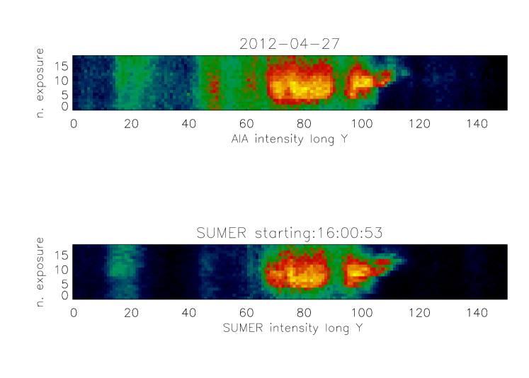
Figure 12: Top: AIA 94 channel intensity along the SUMER slit (x-axes in the figure) as function of exposure number (y-axes in the figure). This is the best solution for the co-alignement. Bottom: Similar to the top plot, but for SUMER Fe XVIII 974.86 Å. Note that the plot does not include the pause between each couple of exposures. The solar limb is on the right side of the image.

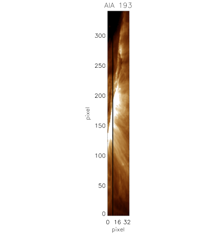
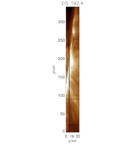
Figure 13: Result of the AIA 193 (left) and EIS 192.4Å (right) alignment for April 27.

Appendix B SUMER stray light

Due to our interest in the hot emission, we estimated the stray light by using the AIA 94 channel data convolved with the SUMER point spread function. The reference image was the integration of two AIA 94 images taken on the 27 April 2012 at 21:42 UT. This resulting image, binned to the SUMER pixel size, was convolved with the instrumental profile (P. Lemaire, private communicaton) as shown in Figure 14 left. On the right plot of Figure 14 we show the horizontal cut (marked by the white line) on this image, scaled to the original AIA image, which crosses the active region and the SUMER field of view. We see that the off-limb stray light is only few percent of the original flux.

We also tested stray light in cool lines. Our data also contain the O I 1152.15 Å  which is a good stray-light marker close to the limb. We integrated over the 60 exposures and extracted the line intensity along the SUMER slit position 2 in those pixels where the SNR is above 10. Assuming that the observed intensity is only due to scattered light in the instrument, we calculated its ratio to the solar value (Curdt et al., 2004; Parenti et al., 2004, 2005), and found that it is always below $3\%$.

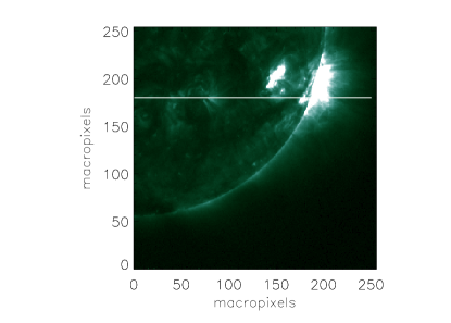
Figure 14: Left: result of the AIA 94 image convolved with the SUMER PSF. This image was divided to the original AIA image to obtain the percentage of stray light in the measured flux. The right plot shows a horizontal cut of this images ratio at the vertical position which is sampled by the SUMER slit. This position is marked on the left plot with a white line.

Appendix C SUMER wavelength calibration

SUMER spectra are not wavelength calibrated and the grating dispersion is wavelength dependent. Ideally, to perform the calibration we need to have reference lines profiles (that are emitted by static features) along the whole waveband. The process is quite straightforward once we have observations targeting the quiet Sun: the SUMER wavebands include a long list of chromospheric lines, including neutrals or singly ionized ions, for which we assume a mean zero velocity (see details of this calibration in Parenti et al. (2004)). This is not the case when we are dealing with off-limb observations in active regions, where the coronal emission dominates, and plasma flows are more common. We tried to minimize the effects of possible local flows applying the following two steps. We used the data from the slit positioned further out in the corona (position 2, mask $G$), averaging the spectra over seventy pixels in the southern part of the slit (that is the area at the greatest distance and in the AR periphery). To produce an average effect which minimizes the detection of flows, we chose as reference lines all the bright ones, independently of their formation temperature. Because of the wavelength dependence of the dispersion, we performed an independent calibration in our three spectral windows. We proceeded by measuring the position of our spectral lines in the pixel dimension on the detector, and used a linear relation and reference positions to convert it in the wavelength space.

Appendix D Electron density along the SUMER slit

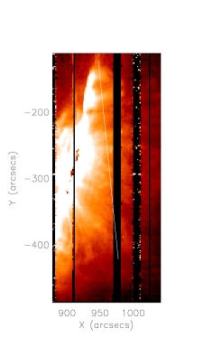
Figure 15: EIS map of density derived from the Fe XIII lines ratio for the raster at 20:24 UT. The intensity has been saturated to highlight the faint off-limb structuring. The SUMER slit is superimposed.

Figure 16: Left and center: electron density derived from the EIS Fe XIII lines ratio along the SUMER slit for position 1 (EIS rasters at 18:18 UT and 20:24 UT respectively). Right: the same but for SUMER slit position 2 (EIS raster starting at 23:01 UT).

We derived the electron density maps from the EIS rasters using the electron density diagnostics of lines ratio described in Section 4. We used Fe XIII $(203.82+203.8)/202.04$ Å ($\log T=6.25$), which is sensitive in the range $N>10^{8}~{}\mathrm{cm^{-3}}$. Figure 15 shows the density map from the raster starting at 20:24 UT on April the 27th (SUMER slit position 1). The density along the SUMER slit derived from this map is shown in the central panel of Figure 16. For SUMER slit position 1 we also have an earlier EIS map and the density profile along the SUMER slit is shown on the left of Figure 16. The right plot in this figure gives the density derived along the SUMER slit for slit position 2.

The two profiles on SUMER position 1 reflect the changing of the structuring of the AR at this temperature about two hours apart. We can identify the same main features with a change in the relative density amplitude, which is most evident in the AR core ($-250\arcsec<Y<-200\arcsec$). This area is the one occupied by the flaring region and by the hot loop visible in the first raster (Figure 12). Note how little these profiles resemble the intensity profiles along the slit of the hot lines, suggesting we are observing different thermal structures along the line of sight. Figure 16 right shows a more important drop in density as Y decreases, due both the increase height above the active region and the increasing distance from the AR core.

The density values found here have been used for the thermal analysis.

Appendix E SUMER temporal variability for slit position 2

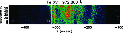
Figure 17: Left: SUMER Fe XVIII intensity along the slit in position 2, plotted for the sixty exposures. Right: time integrated Fe XVII and Fe XVIII intensities along the slit in position 2. The north is on the right side of the plot.

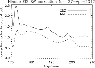
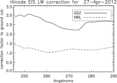
Figure 18: Correction factor to the pre-flight radiometric calibration derived by (Warren et al., 2014) (NRL in the figure) and Del Zanna (2013a) (GDZ in the figure).

Figure 17 left shows the temporal variation of the Fe XVIII along the SUMER slit in position 2. We can notice a general temporal variation of the structures which tend to spatially spread along the slit as the timeline increases. We selected the most stable parts highlighted by the yellow lines (masks $D$, $E$).

Figure 17 right shows the temporal averaged integrated flux of Fe XVII and Fe XVIII, which were taken six hours apart. There is a temporal variation mostly in the core of the AR. We adapted our masks to these changes. As shown in Figure 9 there is no thermal variation within at these locations.

Appendix F EIS radiometric calibration

Figure 18 shows the correction factor to the pre-flight radiometric calibration of EIS for the two channels, as determined by Del Zanna (2013a) (solid line) and Warren et al. (2014) (dashed line) for the period of our observations.

References

- Argiroffi et al. (2008) Argiroffi, C., Peres, G., Orlando, S., & Reale, F. 2008, A&A, 488, 1069
- Barnes et al. (2016) Barnes, W. T., Cargill, P. J., & Bradshaw, S. J. 2016, ApJ, 833, 217
- Brosius et al. (2014) Brosius, J. W., Daw, A. N., & Rabin, D. M. 2014, ApJ, 790, 112
- Cargill (1994) Cargill, P. J. 1994, ApJ, 422, 381
- Cargill (2014) —. 2014, ApJ, 784, 49
- Culhane et al. (2007) Culhane, J. L., Harra, L. K., James, A. M., et al. 2007, Sol. Phys., 243, 19
- Curdt et al. (2004) Curdt, W., Landi, E., & Feldman, U. 2004, A&A, 427, 1045
- Del Zanna (2013a) Del Zanna, G. 2013a, A&A, 555, A47
- Del Zanna (2013b) —. 2013b, A&A, 558, A73
- Del Zanna et al. (2015a) Del Zanna, G., Dere, K. P., Young, P. R., Landi, E., & Mason, H. E. 2015a, A&A, 582, A56
- Del Zanna & Mason (2014) Del Zanna, G., & Mason, H. E. 2014, A&A, 565, A14
- Del Zanna et al. (2015b) Del Zanna, G., Tripathi, D., Mason, H., Subramanian, S., & O’Dwyer, B. 2015b, A&A, 573, A104
- Dere et al. (1997) Dere, K. P., Landi, E., Mason, H. E., Monsignori Fossi, B. C., & Young, P. R. 1997, A&AS, 125, 149
- Dong et al. (2012) Dong, F., Wang, F., Zhong, J., Liang, G., & Zhao, G. 2012, PASJ, 64, 131
- Drake & Kashyap (2010) Drake, J. J., & Kashyap, V. L. 2010, PINTofALE: Package for Interactive Analysis of Line Emission, Astrophysics Source Code Library, , , ascl:1007.001
- Feldman (1992) Feldman, U. 1992, Phys. Scr, 46, 202
- Feldman et al. (1997) Feldman, U., Behring, W. E., Curdt, W., et al. 1997, ApJS, 113, 195
- Freeland & Handy (1998) Freeland, S. L., & Handy, B. N. 1998, Sol. Phys., 182, 497
- Giunta et al. (2012) Giunta, A. S., Fludra, A., O’Mullane, M. G., & Summers, H. P. 2012, A&A, 538, A88
- Golub et al. (2007) Golub, L., Deluca, E., Austin, G., et al. 2007, Sol. Phys., 243, 63
- Guennou et al. (2012) Guennou, C., Auchère, F., Soubrié, E., et al. 2012, ApJS, 203, 26
- Hannah et al. (2016) Hannah, I. G., Grefenstette, B. W., Smith, D. M., et al. 2016, ApJ, 820, L14
- Ishikawa et al. (2014) Ishikawa, S.-n., Glesener, L., Christe, S., et al. 2014, PASJ, 66, S15
- Ivanov-Kholodnyi & Nikol’Skii (1963) Ivanov-Kholodnyi, G. S., & Nikol’Skii, G. M. 1963, Soviet Ast., 6, 609
- Kashyap & Drake (1998) Kashyap, V., & Drake, J. J. 1998, ApJ, 503, 450
- Kashyap & Drake (2000) —. 2000, Bulletin of the Astronomical Society of India, 28, 475
- Klimchuk (2006) Klimchuk, J. A. 2006, Sol. Phys., 234, 41
- Klimchuk (2015) —. 2015, Philosophical Transactions of the Royal Society of London Series A, 373, 20140256
- Ko et al. (2009) Ko, Y.-K., Doschek, G. A., Warren, H. P., & Young, P. R. 2009, ApJ, 697, 1956
- Ko et al. (2016) Ko, Y.-K., Young, P. R., Muglach, K., Warren, H. P., & Ugarte-Urra, I. 2016, ApJ, 826, 126
- Landi & Bhatia (2005) Landi, E., & Bhatia, A. K. 2005, Atomic Data and Nuclear Data Tables, 90, 177
- Landi & Feldman (2008) Landi, E., & Feldman, U. 2008, ApJ, 672, 674
- Landi & Young (2010) Landi, E., & Young, P. R. 2010, ApJ, 714, 636
- Lang et al. (2006) Lang, J., Kent, B. J., Paustian, W., et al. 2006, Appl. Opt., 45, 8689
- McTiernan (2009) McTiernan, J. M. 2009, ApJ, 697, 94
- Miceli et al. (2012) Miceli, M., Reale, F., Gburek, S., et al. 2012, A&A, 544, A139
- Parenti (2015) Parenti, S. 2015, in Astrophysics and Space Science Library, Vol. 415, Solar Prominences, ed. J.-C. Vial & O. Engvold, 61
- Parenti et al. (2006) Parenti, S., Buchlin, E., Cargill, P. J., Galtier, S., & Vial, J.-C. 2006, ApJ, 651, 1219
- Parenti et al. (2010) Parenti, S., Reale, F., & Reeves, K. K. 2010, A&A, 517, A41
- Parenti et al. (2004) Parenti, S., Vial, J.-C., & Lemaire, P. 2004, Sol. Phys., 220, 61
- Parenti et al. (2005) —. 2005, A&A, 443, 679
- Parker (1988) Parker, E. N. 1988, ApJ, 330, 474
- Petralia et al. (2014) Petralia, A., Reale, F., Testa, P., & Del Zanna, G. 2014, A&A, 564, A3
- Pottasch (1963) Pottasch, S. R. 1963, ApJ, 137, 945+
- Reale (2014) Reale, F. 2014, Living Reviews in Solar Physics, 11, 4
- Reale et al. (2011) Reale, F., Guarrasi, M., Testa, P., et al. 2011, ApJ, 736, L16
- Reale et al. (2009a) Reale, F., McTiernan, J. M., & Testa, P. 2009a, ApJ, 704, L58
- Reale et al. (2009b) Reale, F., Testa, P., Klimchuk, J. A., & Susanna Parenti. 2009b, ApJ, 698, 756
- Shestov et al. (2010) Shestov, S. V., Kuzin, S. V., Urnov, A. M., Ul’Yanov, A. S., & Bogachev, S. A. 2010, Astronomy Letters, 36, 44
- Sylwester et al. (2010) Sylwester, B., Sylwester, J., & Phillips, K. J. H. 2010, A&A, 514, A82
- Teriaca et al. (2012) Teriaca, L., Warren, H. P., & Curdt, W. 2012, ApJ, 754, L40
- Testa et al. (2011) Testa, P., Reale, F., Landi, E., DeLuca, E. E., & Kashyap, V. 2011, ApJ, 728, 30
- Wang et al. (2016) Wang, K., Si, R., Dang, W., et al. 2016, ApJS, 223, 3
- Warren et al. (2014) Warren, H. P., Ugarte-Urra, I., & Landi, E. 2014, ApJS, 213, 11
- Warren et al. (2012) Warren, H. P., Winebarger, A. R., & Brooks, D. H. 2012, ApJ, 759, 141
- Weber et al. (2004) Weber, M. A., Deluca, E. E., Golub, L., & Sette, A. L. 2004, in IAU Symposium, Vol. 223, Multi-Wavelength Investigations of Solar Activity, ed. A. V. Stepanov, E. E. Benevolenskaya, & A. G. Kosovichev, 321–328
- Wilhelm et al. (1995) Wilhelm, K., Curdt, W., Marsch, E., et al. 1995, Sol. Phys., 162, 189
- Winebarger et al. (2012) Winebarger, A. R., Warren, H. P., Schmelz, J. T., et al. 2012, ApJ, 746, L17