Kubo-Greenwood Electrical Conductivity Formulation and Implementation for Projector Augmented Wave Datasets

Abstract

As the foundation for a new computational implementation, we survey the calculation of the complex electrical conductivity tensor based on the Kubo-Greenwood (KG) formalism (J. Phys. Soc. Jpn. 12, 570 (1957); Proc. Phys. Soc. 71, 585 (1958)), with emphasis on derivations and technical aspects pertinent to use of projector augmented wave datasets with plane wave basis sets (Phys. Rev. B 50, 17953 (1994)). New analytical results and a full implementation of the KG approach in an open-source Fortran 90 post-processing code for use with Quantum Espresso (J. Phys. Cond. Matt. 21, 395502 (2009)) are presented. Named KGEC ([K]ubo [G]reenwood [E]lectronic [C]onductivity), the code calculates the full complex conductivity tensor (not just the average trace). It supports use of either the original KG formula or the popular one approximated in terms of a Dirac delta function. It provides both Gaussian and Lorentzian representations of the Dirac delta function (though the Lorentzian is preferable on basic grounds). KGEC provides decomposition of the conductivity into intra- and inter-band contributions as well as degenerate state contributions. It calculates the dc conductivity tensor directly. It is MPI parallelized over k-points, bands, and plane waves, with an option to recover the plane wave processes for their use in band parallelization as well. It is designed to provide rapid convergence with respect to $\mathbf{k}$-point density. Examples of its use are given.

1 Introduction

Calculation of transport properties of matter is a venerable but still very active research area in part because of the physical significance of transport coefficients and in part because of the major theoretical and computational challenges involved. The computational goal of the present work is to design algorithms for the calculation of the Kubo-Greenwood (KG) electrical conductivity [1, 2] and implement them as a post-processing tool for the widely used Quantum Espresso [3] (QE) code. We begin by reviewing the state of the art of KG electrical conductivity calculations, with emphasis upon derivations and their technical implications. The computational context of the formulation is projector augmented wave (PAW) datasets used with plane wave (PW) basis sets [4] for the solution of the Kohn-Sham (KS) equations [5]. The resultant new program is named KGEC, from the initial letters of Kubo-Greenwood Electrical Conductivity.

Though the primary goal was computational, that reconsideration of the underlying analysis also has proved fruitful, as will become apparent, for example, in the treatment of contributions of intra-band and degenerate band transitions to the conductivity. Beyond the obvious goal of providing new capability for users of QE, the project also was motivated by the opportunity to include finite-temperature effects via free energy density functionals [6, 7] and to provide benefits from orbital-free density functional theory (DFT) molecular dynamics via the Profess@QE package [8]. The coupling of KGEC with these developments opens a wide range of possibilities for simulations of systems over a wide range of state conditions, e.g. warm dense matter.

Starting with the KG general formula in the next section (Sec. 2) we derive in detail all of the mathematical expressions necessary for a full KG implementation. In Sec. 3 we provide the essential ingredients of the PAW method, followed by derivation of the expression for the matrix elements of the gradient operator (Sec. 3.1). Next, Sec. 4 provides an overview of the work flow in KGEC, its installation, execution, input, output and MPI parallelization. We also present results from various tests in Sec. (5), including a comparison with similar Abinit calculations [9]. Underlying difficulties including numerical problems are discussed in Sec. (6), while remarks and comments about future work are in Sec. (7).

2 The Kubo-Greenwood electrical conductivity formula

2.1 General expression

The KG expression [1, 2] for the frequency-dependent complex electrical conductivity tensor is

$$\sigma(\omega)=i\frac{2e^{2}\hbar^{3}}{m_{e}^{2}V}\sum_{m}\sum_{m^{\prime}}\frac{(f(\epsilon_{m^{\prime}})-f(\epsilon_{m}))}{(\epsilon_{m}-\epsilon_{m^{\prime}})}\frac{\langle{m}|\nabla|{m^{\prime}}\rangle\langle{m^{\prime}}|\nabla|{m}\rangle}{\epsilon_{m}-\epsilon_{m^{\prime}}-\hbar\omega+i\delta/2}$$ (1)

or in more compact form

$$\sigma(\omega)=i\frac{2e^{2}\hbar^{3}}{m_{e}^{2}V}\sum_{m}\sum_{m^{\prime}}\frac{\Delta f_{m^{\prime}m}}{\Delta\epsilon_{mm^{\prime}}}\frac{\langle{m}|\nabla|{m^{\prime}}\rangle\langle{m^{\prime}}|\nabla|{m}\rangle}{(\Delta\epsilon_{mm^{\prime}}-\hbar\omega+i\delta/2)}\;.$$ (2)

Before proceeding, note an unconventional aspect compared to the usual KG presentation. In both equations (1) and (2), the expression $\langle{m}|\nabla|{m^{\prime}}\rangle\langle{m^{\prime}}|\nabla|{m}\rangle$ is a dyadic in the coordinate indices of the gradients. For didactic clarity, in a Cartesian system, Eq. (2) becomes

$$\sigma_{x,z}(\omega)=i\frac{2e^{2}\hbar^{3}}{m_{e}^{2}V}\sum_{m}\sum_{m^{\prime}}\frac{\Delta f_{m^{\prime}m}}{\Delta\epsilon_{mm^{\prime}}}\frac{\langle{m}|{\frac{\partial}{\partial x}}|{m^{\prime}}\rangle\langle{m^{\prime}}|{\frac{\partial}{\partial z}}|{m}\rangle}{(\Delta\epsilon_{mm^{\prime}}-\hbar\omega+i\delta/2)}$$ (3)

for the $x$-$z$ element of the conductivity tensor. The more familiar version comes from taking the trace.

In these expressions $m$, $m^{\prime}$ label non-spin-polarized single-particle states with $\epsilon_{m}$, $\epsilon_{m^{\prime}}$ the corresponding eigenvalues and associated Fermi-Dirac occupation numbers $f(\epsilon_{m})$, $f(\epsilon_{m^{\prime}})$. (For simplicity of notation, the temperature is suppressed for now.) In practice and in our implementation, the states and occupations are from a KS DFT calculation, though the analysis presented in this section and the next one does not depend upon that particular choice of mean-field Hamiltonian. (Note that because of the spin-unpolarized formulation, the net occupation of each KS orbital is $2f(\epsilon_{m})$.) Then $\Delta\epsilon_{mm^{\prime}}=\epsilon_{m}-\epsilon_{m^{\prime}}$ and $\Delta f_{m^{\prime}m}=f(\epsilon_{m^{\prime}})-f(\epsilon_{m})$. The constants $e$, $\hbar$, $m_{e}$ and $V$ are the electron charge, Planck’s constant, electron mass, and system volume, respectively. The $i\delta/2$ is an imaginary factor related to damping or relaxation effects. In the Drude model for the electrical conductivity, it is identified with the inverse of the average inter-collision time.

If the matrix element dyadic product $\langle{m}|\nabla|{m^{\prime}}\rangle\langle{m^{\prime}}|\nabla|{m}\rangle$ is real, the real and imaginary parts of $\sigma(\omega)$ can be separated by multiplying and dividing by $(\Delta\epsilon_{mm^{\prime}}-\hbar\omega-i\delta/2)$, leading to

$$\sigma(\omega)=\sigma_{1}(\omega)+i\sigma_{2}(\omega),$$ (4)

with

$$\sigma_{1}(\omega)=\frac{2e^{2}\hbar^{3}}{m_{e}^{2}V}\sum_{m}\sum_{m^{\prime}}\frac{\Delta f_{m^{\prime}m}}{\Delta\epsilon_{mm^{\prime}}}\langle{m}|\nabla|{m^{\prime}}\rangle\langle{m^{\prime}}|\nabla|{m}\rangle\frac{\delta/2}{(\Delta\epsilon_{mm^{\prime}}-\hbar\omega)^{2}+\delta^{2}/4}$$ (5)

and

$$\sigma_{2}(\omega)=\frac{2e^{2}\hbar^{3}}{m_{e}^{2}V}\sum_{m}\sum_{m^{\prime}}\frac{\Delta f_{m^{\prime}m}}{\Delta\epsilon_{mm^{\prime}}}\langle{m}|\nabla|{m^{\prime}}\rangle\langle{m^{\prime}}|\nabla|{m}\rangle\frac{(\Delta\epsilon_{mm^{\prime}}-\hbar\omega)}{(\Delta\epsilon_{mm^{\prime}}-\hbar\omega)^{2}+\delta^{2}/4}.$$ (6)

Again be reminded that both $\sigma_{1}$ and $\sigma_{2}$ are tensors, not scalars.

Commonly it is argued that for small $\delta$, the Lorentzian in $\sigma_{1}(\omega)$ behaves like a Dirac delta function, that is

$$\frac{\delta/2}{(\Delta\epsilon_{mm^{\prime}}-\hbar\omega)^{2}+\delta^{2}/4}\approx\pi\delta(\Delta\epsilon_{mm^{\prime}}-\hbar\omega),$$ (7)

which allows $\sigma_{1}(\omega)$ to be written as

$$\sigma_{1}(\omega)=\frac{2\pi e^{2}\hbar^{3}}{m_{e}^{2}V}\sum_{m}\sum_{m^{\prime}}\frac{\Delta f_{m^{\prime}m}}{\Delta\epsilon_{mm^{\prime}}}\langle{m}|\nabla|{m^{\prime}}\rangle\langle{m^{\prime}}|\nabla|{m}\rangle\delta(\Delta\epsilon_{mm^{\prime}}-\hbar\omega),$$ (8)

or

$$\sigma_{1}(\omega)=\frac{2\pi e^{2}\hbar^{2}}{m_{e}^{2}V\omega}\sum_{m}\sum_{m^{\prime}}\Delta f_{m^{\prime}m}\langle{m}|\nabla|{m^{\prime}}\rangle\langle{m^{\prime}}|\nabla|{m}\rangle\delta(\Delta\epsilon_{mm^{\prime}}-\hbar\omega).$$ (9)

Both forms commonly are encountered. We will label Eq. (8) “the Dirac-delta form” (notation “D-d”) or “the exact form or expression”. Note that if one starts with it and represents the Dirac delta function by a Lorentzian, the original Kubo-Greenwood expression is recovered. Similarly Eq. (9) will be labeled “the approximated formula or expression” because one cannot recover the exact Kubo-Greenwood formula from it by simple substitution for the delta function.

In computation, the Dirac delta function in $\sigma_{1}$ often is represented by a Gaussian, even though its natural representation is a Lorentzian. Distinctions among these representations should disappear as $\delta\rightarrow 0$, but in practice they are manifest even for a small, non-zero $\delta$. We return to that in the discussion of numerical tests in Sec. (5). Notice also that, because $\omega>0$ the Dirac delta function in Eq. (9) selects only states with positive energy differences, but the original expression included contributions from states with negative energy differences. That discrepancy can be resolved by introduction of the $\delta(\Delta\epsilon_{mm^{\prime}}+\hbar\omega)$ term as well. Another problem is that only non-degenerate inter-band contributions are included in the approximated formula. We return to that below as well.

2.2 KG formula in the Bloch picture

We focus on periodic systems, so the state indices $m$ and $m^{\prime}$ become band index and Brillouin zone wave vector pairs $n,\mathbf{k}$ and $n^{\prime},\mathbf{k^{\prime}}$ for Bloch states. Because the gradient matrix elements between $\mathbf{k}$ and $\mathbf{k^{\prime}}$ states are zero if $\mathbf{k}\neq\mathbf{k^{\prime}}$, the KG formulae, (Eqs. (5) and (6)), become

$$\tilde{\sigma}_{1}(\omega)=\frac{2e^{2}\hbar^{3}}{m_{e}^{2}\Omega}\sum_{\mathbf{k}}w_{\mathbf{k}}\sum_{nn^{\prime}}\frac{\Delta f_{n^{\prime}\mathbf{k},n\mathbf{k}}}{\Delta\epsilon_{n\mathbf{k},n^{\prime}\mathbf{k}}}\langle{\Psi_{n\mathbf{k}}}|\nabla|{\Psi_{n^{\prime}\mathbf{k}}}\rangle\langle{\Psi_{n^{\prime}\mathbf{k}}}|\nabla|{\Psi_{n\mathbf{k}}}\rangle\frac{\delta/2}{(\Delta\epsilon_{n\mathbf{k},n^{\prime}\mathbf{k}}-\hbar\omega)^{2}+\delta^{2}/4}$$ (10)

and

$$\tilde{\sigma}_{2}(\omega)=\frac{2e^{2}\hbar^{3}}{m_{e}^{2}\Omega}\sum_{\mathbf{k}}w_{\mathbf{k}}\sum_{nn^{\prime}}\frac{\Delta f_{n^{\prime}\mathbf{k},n\mathbf{k}}}{\Delta\epsilon_{n\mathbf{k},n^{\prime}\mathbf{k}}}\langle{\Psi_{n\mathbf{k}}}|\nabla|{\Psi_{n^{\prime}\mathbf{k}}}\rangle\langle{\Psi_{n^{\prime}\mathbf{k}}}|\nabla|{\Psi_{n\mathbf{k}}}\rangle\frac{(\Delta\epsilon_{n\mathbf{k},n^{\prime}\mathbf{k}}-\hbar\omega)}{(\Delta\epsilon_{n\mathbf{k},n^{\prime}\mathbf{k}}-\hbar\omega)^{2}+\delta^{2}/4}\;.$$ (11)

Here $\Omega$ is the unit cell volume and $w_{\mathbf{k}}$ are the $\mathbf{k}$-point integration weights. We have also used a tilde ~ atop the $\sigma$s to highlight that they both become complex because the matrix element tensor product no longer is necessarily real (since the Bloch wave functions are, in the most general case, complex).

Both $\sigma_{1}$ and $\sigma_{2}$ can be recovered by means of the elementary relations ${\sigma}_{1}(\omega)=\Re(\tilde{\sigma_{1}}+i\tilde{\sigma_{2}})$, ${\sigma}_{2}(\omega)=\Im(\tilde{\sigma_{1}}+i\tilde{\sigma_{2}})$ and use of the fact that the real part of $\sigma$ must be even and the imaginary part odd with respect to $\omega$. It follows that

$${\sigma}_{1}(\omega) =\Re(\tilde{\sigma}_{1}(\omega))-\Im(\tilde{\sigma}_{2}(\omega))=\Re(\tilde{\sigma}_{1}(\omega))$$ (12)

$$=\frac{2e^{2}\hbar^{3}}{m_{e}^{2}\Omega}\sum_{\mathbf{k}}w_{\mathbf{k}}\sum_{nn^{\prime}}\frac{\Delta f_{n^{\prime}\mathbf{k},n\mathbf{k}}}{\Delta\epsilon_{n\mathbf{k},n^{\prime}\mathbf{k}}}\Re{(\langle{\Psi_{n\mathbf{k}}}|\nabla|{\Psi_{n^{\prime}\mathbf{k}}}\rangle\langle{\Psi_{n^{\prime}\mathbf{k}}}|\nabla|{\Psi_{n\mathbf{k}}}\rangle)}\frac{\delta/2}{(\Delta\epsilon_{n\mathbf{k},n^{\prime}\mathbf{k}}-\hbar\omega)^{2}+\delta^{2}/4}$$ (13)

and

$${\sigma}_{2}(\omega) =\Im(\tilde{\sigma}_{1}(\omega))+\Re(\tilde{\sigma}_{2}(\omega))=\Re(\tilde{\sigma}_{2}(\omega))$$ (14)

$$=\frac{2e^{2}\hbar^{3}}{m_{e}^{2}\Omega}\sum_{\mathbf{k}}w_{\mathbf{k}}\sum_{nn^{\prime}}\frac{\Delta f_{n^{\prime}\mathbf{k},n\mathbf{k}}}{\Delta\epsilon_{n\mathbf{k},n^{\prime}\mathbf{k}}}\Re{(\langle{\Psi_{n\mathbf{k}}}|\nabla|{\Psi_{n^{\prime}\mathbf{k}}}\rangle\langle{\Psi_{n^{\prime}\mathbf{k}}}|\nabla|{\Psi_{n\mathbf{k}}}\rangle)}\frac{(\Delta\epsilon_{n\mathbf{k},n^{\prime}\mathbf{k}}-\hbar\omega)}{(\Delta\epsilon_{n\mathbf{k},n^{\prime}\mathbf{k}}-\hbar\omega)^{2}+\delta^{2}/4}\;.$$ (15)

Sum rules also emerge, to wit

$$\sum_{\mathbf{k}}w_{\mathbf{k}}\sum_{nn^{\prime}}\frac{\Delta f_{n\mathbf{k},n^{\prime}\mathbf{k}}}{\Delta\epsilon_{n\mathbf{k},n^{\prime}\mathbf{k}}}\Im{(\langle{\Psi_{n\mathbf{k}}}|\nabla|{\Psi_{n^{\prime}\mathbf{k}}}\rangle\langle{\Psi_{n^{\prime}\mathbf{k}}}|\nabla|{\Psi_{n\mathbf{k}}}\rangle)}\frac{\delta/2}{(\Delta\epsilon_{n\mathbf{k},n^{\prime}\mathbf{k}}-\hbar\omega)^{2}+\delta^{2}/4}=0$$ (16)

and

$$\sum_{\mathbf{k}}w_{\mathbf{k}}\sum_{nn^{\prime}}\frac{\Delta f_{n\mathbf{k},n^{\prime}\mathbf{k}}}{\Delta\epsilon_{n\mathbf{k},n^{\prime}\mathbf{k}}}\Im{(\langle{\Psi_{n\mathbf{k}}}|\nabla|{\Psi_{n^{\prime}\mathbf{k}}}\rangle\langle{\Psi_{n^{\prime}\mathbf{k}}}|\nabla|{\Psi_{n\mathbf{k}}}\rangle)}\frac{(\Delta\epsilon_{n\mathbf{k},n^{\prime}\mathbf{k}}-\hbar\omega)}{(\Delta\epsilon_{n\mathbf{k},n^{\prime}\mathbf{k}}-\hbar\omega)^{2}+\delta^{2}/4}=0.$$ (17)

We return to them below.

In correspondence with the general KG formulae of the preceding section, for the solid we have the D-d form

$${\sigma}_{1}^{D-d}(\omega)=\frac{2\pi e^{2}\hbar^{3}}{m_{e}^{2}\Omega}\sum_{\mathbf{k}}w_{\mathbf{k}}\sum_{nn^{\prime}}\frac{\Delta f_{n^{\prime}\mathbf{k},n\mathbf{k}}}{\Delta\epsilon_{n\mathbf{k},n^{\prime}\mathbf{k}}}\,\Re{(\langle{\Psi_{n\mathbf{k}}}|\nabla|{\Psi_{n^{\prime}\mathbf{k}}}\rangle\langle{\Psi_{n^{\prime}\mathbf{k}}}|\nabla|{\Psi_{n\mathbf{k}}}\rangle)}\,\delta(\Delta\epsilon_{n\mathbf{k},n^{\prime}\mathbf{k}}-\hbar\omega)$$ (18)

and the approximated form

$${\sigma}_{1}^{a}(\omega)=\frac{2\pi e^{2}\hbar^{2}}{m_{e}^{2}\Omega\omega}\sum_{\mathbf{k}}w_{\mathbf{k}}\sum_{nn^{\prime}}{\Delta f_{n^{\prime}\mathbf{k},n\mathbf{k}}}\,\Re{(\langle{\Psi_{n\mathbf{k}}}|\nabla|{\Psi_{n^{\prime}\mathbf{k}}}\rangle\langle{\Psi_{n^{\prime}\mathbf{k}}}|\nabla|{\Psi_{n\mathbf{k}}}\rangle)}\,\delta(\Delta\epsilon_{n\mathbf{k},n^{\prime}\mathbf{k}}-\hbar\omega).$$ (19)

For calculations it may be numerically advantageous to enforce the even parity of $\sigma_{1}$ and use

$$\sigma_{1,calculated}(\omega)=\frac{1}{2}[\sigma_{1}(\omega)+\sigma_{1}(-\omega)]\;.$$ (20)

2.2.1 Intra-band, degenerate state, and inter-band contributions

Practical use of the foregoing conductivity formulae requires resolution of the potential problems associated with $\Delta\epsilon_{n\mathbf{k},n^{\prime}\mathbf{k}}$ going to zero. For that we return to Eq. (13) and separate the sums over band indices $n$ and $n^{\prime}$ into one over $n=n^{\prime}$, a second one for $n\neq n^{\prime}$ and $\Delta\epsilon_{n\mathbf{k},n^{\prime}\mathbf{k}}=0$, and a third sum for $n\neq n^{\prime}$ and $\Delta\epsilon_{n\mathbf{k},n^{\prime}\mathbf{k}}\neq 0$, To treat the singularities in the first two sums, we add an infinitesimal energy $\varepsilon$ and consider $\varepsilon\rightarrow 0$. Details are

$$\sum_{nn^{\prime}}\frac{\Delta f_{n^{\prime}\mathbf{k},n\mathbf{k}}}{\Delta\epsilon_{n\mathbf{k},n^{\prime}\mathbf{k}}}\Re{(\langle{\Psi_{n\mathbf{k}}}|\nabla|{\Psi_{n^{\prime}\mathbf{k}}}\rangle\langle{\Psi_{n^{\prime}\mathbf{k}}}|\nabla|{\Psi_{n\mathbf{k}}}\rangle)}\frac{\delta/2}{(\Delta\epsilon_{n\mathbf{k},n^{\prime}\mathbf{k}}-\hbar\omega)^{2}+\delta^{2}/4}$$

$$= \lim_{\varepsilon\rightarrow 0}\sum_{n}\frac{f(\epsilon_{n\mathbf{k}})-f(\epsilon_{n\mathbf{k}}+\varepsilon)}{\varepsilon}{\Re(\langle{\Psi_{n\mathbf{k}}}|\nabla|{\Psi_{n\mathbf{k}}}\rangle\langle{\Psi_{n\mathbf{k}}}|\nabla|{\Psi_{n\mathbf{k}}}\rangle)}\frac{\delta/2}{(\varepsilon-\hbar\omega)^{2}+\delta^{2}/4}$$

$$+ \lim_{\varepsilon\rightarrow 0}\sum_{\begin{subarray}{c}n\neq n^{\prime}\\ \epsilon_{n\mathbf{k}}=\epsilon_{n^{\prime}\mathbf{k}}\end{subarray}}\frac{f(\epsilon_{n\mathbf{k}})-f(\epsilon_{n\mathbf{k}}+\varepsilon)}{\varepsilon}{\Re(\langle{\Psi_{n\mathbf{k}}}|\nabla|{\Psi_{n^{\prime}\mathbf{k}}}\rangle\langle{\Psi_{n^{\prime}\mathbf{k}}}|\nabla|{\Psi_{n\mathbf{k}}}\rangle)}\frac{\delta/2}{(\varepsilon-\hbar\omega)^{2}+\delta^{2}/4}$$

$$+ \sum_{\begin{subarray}{c}n\neq n^{\prime}\\ \epsilon_{n\mathbf{k}}\neq\epsilon_{n^{\prime}\mathbf{k}}\end{subarray}}\frac{\Delta f_{n^{\prime}\mathbf{k},n\mathbf{k}}}{\Delta\epsilon_{n\mathbf{k},n^{\prime}\mathbf{k}}}{\Re(\langle{\Psi_{n\mathbf{k}}}|\nabla|{\Psi_{n^{\prime}\mathbf{k}}}\rangle\langle{\Psi_{n^{\prime}\mathbf{k}}}|\nabla|{\Psi_{n\mathbf{k}}}\rangle)}\frac{\delta/2}{(\Delta\epsilon_{n\mathbf{k},n^{\prime}\mathbf{k}}-\hbar\omega)^{2}+\delta^{2}/4}\;.$$ (21)

Taking the limits reduces the expression to

$$\sum_{nn^{\prime}}\frac{\Delta f_{n^{\prime}\mathbf{k},n\mathbf{k}}}{\Delta\epsilon_{n\mathbf{k},n^{\prime}\mathbf{k}}}{\Re(\langle{\Psi_{n\mathbf{k}}}|\nabla|{\Psi_{n^{\prime}\mathbf{k}}}\rangle\langle{\Psi_{n^{\prime}\mathbf{k}}}|\nabla|{\Psi_{n\mathbf{k}}}\rangle)}\frac{\delta/2}{(\Delta\epsilon_{n\mathbf{k},n^{\prime}\mathbf{k}}-\hbar\omega)^{2}+\delta^{2}/4}$$

$$= -\sum_{n}\frac{\partial f(\epsilon_{n\mathbf{k}})}{\partial\epsilon_{n\mathbf{k}}}{\Re(\langle{\Psi_{n\mathbf{k}}}|\nabla|{\Psi_{n\mathbf{k}}}\rangle\langle{\Psi_{n\mathbf{k}}}|\nabla|{\Psi_{n\mathbf{k}}}\rangle)}\frac{\delta/2}{(\hbar\omega)^{2}+\delta^{2}/4}$$

$$- \sum_{\begin{subarray}{c}n\neq n^{\prime}\\ \epsilon_{n\mathbf{k}}=\epsilon_{n^{\prime}\mathbf{k}}\end{subarray}}\frac{\partial f(\epsilon_{n\mathbf{k}})}{\partial\epsilon_{n\mathbf{k}}}{\Re(\langle{\Psi_{n\mathbf{k}}}|\nabla|{\Psi_{n^{\prime}\mathbf{k}}}\rangle\langle{\Psi_{n^{\prime}\mathbf{k}}}|\nabla|{\Psi_{n\mathbf{k}}}\rangle)}\frac{\delta/2}{(\hbar\omega)^{2}+\delta^{2}/4}$$

$$+ \sum_{\begin{subarray}{c}n\neq n^{\prime}\\ \epsilon_{n\mathbf{k}}\neq\epsilon_{n^{\prime}\mathbf{k}}\end{subarray}}\frac{\Delta f_{n^{\prime}\mathbf{k},n\mathbf{k}}}{\Delta\epsilon_{n\mathbf{k},n^{\prime}\mathbf{k}}}{\Re(\langle{\Psi_{n\mathbf{k}}}|\nabla|{\Psi_{n^{\prime}\mathbf{k}}}\rangle\langle{\Psi_{n^{\prime}\mathbf{k}}}|\nabla|{\Psi_{n\mathbf{k}}}\rangle)}\frac{\delta/2}{(\Delta\epsilon_{n\mathbf{k},n^{\prime}\mathbf{k}}-\hbar\omega)^{2}+\delta^{2}/4}\;.$$ (22)

The result is

$${\sigma}_{1}(\omega)=-\frac{2e^{2}\hbar^{3}}{m_{e}^{2}\Omega}\sum_{\mathbf{k}}w_{\mathbf{k}}\Big{[} \sum_{n}\frac{\partial f(\epsilon_{n\mathbf{k}})}{\partial\epsilon_{n\mathbf{k}}}{\Re(\langle{\Psi_{n\mathbf{k}}}|\nabla|{\Psi_{n\mathbf{k}}}\rangle\langle{\Psi_{n\mathbf{k}}}|\nabla|{\Psi_{n\mathbf{k}}}\rangle)}\frac{\delta/2}{(\hbar\omega)^{2}+\delta^{2}/4}$$

$$+\sum_{\begin{subarray}{c}n\neq n^{\prime}\\ \epsilon_{n\mathbf{k}}=\epsilon_{n^{\prime}\mathbf{k}}\end{subarray}}\frac{\partial f(\epsilon_{n\mathbf{k}})}{\partial\epsilon_{n\mathbf{k}}}{\Re(\langle{\Psi_{n\mathbf{k}}}|\nabla|{\Psi_{n^{\prime}\mathbf{k}}}\rangle\langle{\Psi_{n^{\prime}\mathbf{k}}}|\nabla|{\Psi_{n\mathbf{k}}}\rangle)}\frac{\delta/2}{(\hbar\omega)^{2}+\delta^{2}/4}$$

$$- \sum_{\begin{subarray}{c}n\neq n^{\prime}\\ \epsilon_{n\mathbf{k}}\neq\epsilon_{n^{\prime}\mathbf{k}}\end{subarray}}\frac{\Delta f_{n^{\prime}\mathbf{k},n\mathbf{k}}}{\Delta\epsilon_{n\mathbf{k},n^{\prime}\mathbf{k}}}{\Re(\langle{\Psi_{n\mathbf{k}}}|\nabla|{\Psi_{n^{\prime}\mathbf{k}}}\rangle\langle{\Psi_{n^{\prime}\mathbf{k}}}|\nabla|{\Psi_{n\mathbf{k}}}\rangle)}\frac{\delta/2}{(\Delta\epsilon_{n\mathbf{k},n^{\prime}\mathbf{k}}-\hbar\omega)^{2}+\delta^{2}/4}\Big{]}.$$ (23)

Similarly for $\sigma_{2}$ we have

$${\sigma}_{2}(\omega)=-\frac{2e^{2}\hbar^{3}}{m_{e}^{2}\Omega}\sum_{\mathbf{k}}w_{\mathbf{k}}\Big{[} \sum_{n}\frac{\partial f(\epsilon_{n\mathbf{k}})}{\partial\epsilon_{n\mathbf{k}}}{\Re(\langle{\Psi_{n\mathbf{k}}}|\nabla|{\Psi_{n\mathbf{k}}}\rangle\langle{\Psi_{n\mathbf{k}}}|\nabla|{\Psi_{n\mathbf{k}}}\rangle)}\frac{\hbar\omega}{(\hbar\omega)^{2}+\delta^{2}/4}$$

$$+ \sum_{\begin{subarray}{c}n\neq n^{\prime}\\ \epsilon_{n\mathbf{k}}=\epsilon_{n^{\prime}\mathbf{k}}\end{subarray}}\frac{\partial f(\epsilon_{n\mathbf{k}})}{\partial\epsilon_{n\mathbf{k}}}{\Re(\langle{\Psi_{n\mathbf{k}}}|\nabla|{\Psi_{n^{\prime}\mathbf{k}}}\rangle\langle{\Psi_{n^{\prime}\mathbf{k}}}|\nabla|{\Psi_{n\mathbf{k}}}\rangle)}\frac{\hbar\omega}{(\hbar\omega)^{2}+\delta^{2}/4}$$

$$- \sum_{\begin{subarray}{c}n\neq n^{\prime}\\ \epsilon_{n\mathbf{k}}\neq\epsilon_{n^{\prime}\mathbf{k}}\end{subarray}}\frac{\Delta f_{n^{\prime}\mathbf{k},n\mathbf{k}}}{\Delta\epsilon_{n\mathbf{k},n^{\prime}\mathbf{k}}}{\Re(\langle{\Psi_{n\mathbf{k}}}|\nabla|{\Psi_{n^{\prime}\mathbf{k}}}\rangle\langle{\Psi_{n^{\prime}\mathbf{k}}}|\nabla|{\Psi_{n\mathbf{k}}}\rangle)}\frac{(\Delta\epsilon_{n\mathbf{k},n^{\prime}\mathbf{k}}-\hbar\omega)}{(\Delta\epsilon_{n\mathbf{k},n^{\prime}\mathbf{k}}-\hbar\omega)^{2}+\delta^{2}/4}\Big{]}.$$ (24)

The occupation number derivatives $\partial f(\epsilon_{n\mathbf{k}})/\partial\epsilon_{n\mathbf{k}}$ have been discussed in the closely related setting of density functional perturbation theory [10] and in consideration of intra-band contributions in the KG context [11]. So far as we can tell, a full treatment for the KG formalism leading to the appearance of such derivatives from both intra-band transitions and from degeneracies has not been presented. Note that there has been work on deriving the intra-band contributions using a band dispersion linearization technique [12].

2.2.2 Drude and dc components

A brief detour is useful. If the inter-band, non-degenerate contribution is negligible for small $\omega$, then only the first two sums in Eq. (23) contribute to the total and therefore we can write

$$\sigma_{1}^{D}(\omega) =-\frac{2e^{2}\hbar^{3}}{m_{e}^{2}\Omega}\frac{\delta/2}{(\hbar\omega)^{2}+\delta^{2}/4}$$

$$\times\sum_{\mathbf{k}}w_{\mathbf{k}}\Big{[}\sum_{n}\frac{\partial f(\epsilon_{n\mathbf{k}})}{\partial\epsilon_{n\mathbf{k}}}\Re{(\langle{\Psi_{n\mathbf{k}}}|\nabla|{\Psi_{n\mathbf{k}}}\rangle\langle{\Psi_{n\mathbf{k}}}|\nabla|{\Psi_{n\mathbf{k}}}\rangle)}$$

$$+ \sum_{n\neq n^{\prime}}\delta_{\epsilon_{n\mathbf{k}}\epsilon_{n^{\prime}\mathbf{k}}}\frac{\partial f(\epsilon_{n\mathbf{k}})}{\partial\epsilon_{n\mathbf{k}}}\Re{(\langle{\Psi_{n\mathbf{k}}}|\nabla|{\Psi_{n^{\prime}\mathbf{k}}}\rangle\langle{\Psi_{n^{\prime}\mathbf{k}}}|\nabla|{\Psi_{n\mathbf{k}}}\rangle)}\Big{]}\;.$$ (25)

If we identify the average inter-collision time as

$$\tau=2\hbar/\delta$$ (26)

and the effective charge-to-mass ratio as

$$\left(\frac{n_{e}}{m_{e}}\right)_{eff} =-\frac{2e^{2}\hbar^{2}}{m_{e}^{2}\Omega}\sum_{\mathbf{k}}w_{\mathbf{k}}\left[\sum_{n}\frac{\partial f(\epsilon_{n\mathbf{k}})}{\partial\epsilon_{n\mathbf{k}}}\Re{(\langle{\Psi_{n\mathbf{k}}}|\nabla|{\Psi_{n\mathbf{k}}}\rangle\langle{\Psi_{n\mathbf{k}}}|\nabla|{\Psi_{n\mathbf{k}}}\rangle)}\right.$$

$$+\left.\sum_{yn\neq n^{\prime}}\delta_{\epsilon_{n\mathbf{k}}\epsilon_{n^{\prime}\mathbf{k}}}\frac{\partial f(\epsilon_{n\mathbf{k}})}{\partial\epsilon_{n\mathbf{k}}}\Re{(\langle{\Psi_{n\mathbf{k}}}|\nabla|{\Psi_{n^{\prime}\mathbf{k}}}\rangle\langle{\Psi_{n^{\prime}\mathbf{k}}}|\nabla|{\Psi_{n\mathbf{k}}}\rangle)}\right]\;,$$ (27)

then Eq. (25) becomes the Drude expression [13, 11]

$$\sigma_{1}^{D}(\omega)=\frac{\left(\frac{n_{e}}{m_{e}}\right)_{eff}\tau}{1+(\omega\tau)^{2}}.$$ (28)

The limit $\omega\rightarrow 0$ yields the direct current (dc) conductivity tensor in the Drude approximation

$$\sigma_{dc}^{D}=-\frac{2e^{2}\hbar^{2}\tau}{m_{e}^{2}\Omega}\sum_{\mathbf{k}}w_{\mathbf{k}}\Big{[} \sum_{n}\frac{\partial f(\epsilon_{n\mathbf{k}})}{\partial\epsilon_{n\mathbf{k}}}\Re{(\langle{\Psi_{n\mathbf{k}}}|\nabla|{\Psi_{n\mathbf{k}}}\rangle\langle{\Psi_{n\mathbf{k}}}|\nabla|{\Psi_{n\mathbf{k}}}\rangle)}$$

$$+ \sum_{n\neq n^{\prime}}\delta_{\epsilon_{n\mathbf{k}}\epsilon_{n^{\prime}\mathbf{k}}}\frac{\partial f(\epsilon_{n\mathbf{k}})}{\partial\epsilon_{n\mathbf{k}}}\Re{(\langle{\Psi_{n\mathbf{k}}}|\nabla|{\Psi_{n^{\prime}\mathbf{k}}}\rangle\langle{\Psi_{n^{\prime}\mathbf{k}}}|\nabla|{\Psi_{n\mathbf{k}}}\rangle)}\Big{]}.$$ (29)

2.2.3 Exact dc component

Without invoking the Drude approximation, simply taking the limit $\omega\rightarrow 0$ in Eq. (23) gives

$${\sigma}_{dc}=-\frac{2e^{2}\hbar^{3}}{m_{e}^{2}\Omega} \sum_{\mathbf{k}}w_{\mathbf{k}}\Big{[}\frac{2}{\delta}\sum_{n}\frac{\partial f(\epsilon_{n\mathbf{k}})}{\partial\epsilon_{n\mathbf{k}}}\Re{(\langle{\Psi_{n\mathbf{k}}}|\nabla|{\Psi_{n\mathbf{k}}}\rangle\langle{\Psi_{n\mathbf{k}}}|\nabla|{\Psi_{n\mathbf{k}}}\rangle)}$$

$$+ \frac{2}{\delta}\sum_{\begin{subarray}{c}n\neq n^{\prime}\\ \epsilon_{n\mathbf{k}}=\epsilon_{n^{\prime}\mathbf{k}}\end{subarray}}\frac{\partial f(\epsilon_{n\mathbf{k}})}{\partial\epsilon_{n\mathbf{k}}}\Re{(\langle{\Psi_{n\mathbf{k}}}|\nabla|{\Psi_{n^{\prime}\mathbf{k}}}\rangle\langle{\Psi_{n^{\prime}\mathbf{k}}}|\nabla|{\Psi_{n\mathbf{k}}}\rangle)}$$

$$- \sum_{\begin{subarray}{c}n\neq n^{\prime}\\ \epsilon_{n\mathbf{k}}\neq\epsilon_{n^{\prime}\mathbf{k}}\end{subarray}}\frac{\Delta f_{n^{\prime}\mathbf{k},n\mathbf{k}}}{\Delta\epsilon_{n\mathbf{k},n^{\prime}\mathbf{k}}}\Re{(\langle{\Psi_{n\mathbf{k}}}|\nabla|{\Psi_{n^{\prime}\mathbf{k}}}\rangle\langle{\Psi_{n^{\prime}\mathbf{k}}}|\nabla|{\Psi_{n\mathbf{k}}}\rangle)}\frac{\delta/2}{(\Delta\epsilon_{n\mathbf{k},n^{\prime}\mathbf{k}})^{2}+\delta^{2}/4}\Big{]}\;.$$ (30)

This expression includes all possible contributions to the dc conductivity, in contrast with Eq. (29), which omits the non-degenerate inter-band contributions.

2.3 Sum rules

Clearly a key ingredient in the KG conductivity is the set of gradient operator matrix elements. Computing them is a seemingly simple task that can be complicated by procedures (e.g. PAWs; see below) used in the underlying KS calculations. Knowledge of the exact behavior of matrix element sums therefore has been used to test both implementations and calculations. Such sum rules are developed in this section and discussed in terms of their use as possible quality measures of an implementation or accuracy measures of results.

2.3.1 Sum rule in terms of $\hat{\mathbf{r}}$

A seemingly round-about but fruitful way to begin is to use the commutator relation for the Cartesian component $\alpha$ of the position operator with the Hamiltonian $\hat{H}$

$$[\hat{{r}}_{\alpha},\hat{H}]=i\frac{\hbar}{m_{e}}\hat{{p}}_{\alpha}.$$ (31)

Then for the double commutator we have

$$[\hat{{r}}_{\alpha},[\hat{{r}}_{\alpha},\hat{H}]]=i\frac{\hbar}{m_{e}}[\hat{{r}}_{\alpha},\hat{{p}}_{\alpha}]=-\frac{\hbar^{2}}{m_{e}}.$$ (32)

Formation of matrix elements of Eq. (32) taken with $\langle{m}|$ from the left and $|{n}\rangle$ from the right and use of the completeness relation $\sum_{m^{\prime}}|{m^{\prime}}\rangle\langle{m^{\prime}}|=\hat{I}$ gives

$$\sum_{m^{\prime}}\left(\langle{m}|\hat{{r}}_{\alpha}|{m^{\prime}}\rangle\langle{m^{\prime}}|[\hat{{r}}_{\alpha},\hat{H}]|{n}\rangle-\langle{m}|[\hat{{r}}_{\alpha},\hat{H}]|{m^{\prime}}\rangle\langle{m^{\prime}}|\hat{{r}}_{\alpha}|{n}\rangle\right)=-\frac{\hbar^{2}}{m_{e}}\langle{m}|{n}\rangle\;.$$ (33)

This reduces to the general sum rule for each Cartesian component of $\hat{\mathbf{r}}$

$$\sum_{m^{\prime}}(2\epsilon_{m^{\prime}}-\epsilon_{n}-\epsilon_{m})\langle{m}|\hat{{r}}_{\alpha}|{m^{\prime}}\rangle\langle{m^{\prime}}|\hat{{r}}_{\alpha}|{n}\rangle=\frac{\hbar^{2}}{m_{e}}\delta_{mn}.$$ (34)

In particular, for $m=n$ we have the sum rule

$$2\sum_{m^{\prime}}(\epsilon_{m^{\prime}}-\epsilon_{m})|\langle{m^{\prime}}|\hat{{r}}_{\alpha}|{m}\rangle|^{2}=\frac{\hbar^{2}}{m_{e}}.$$ (35)

or

$$2\sum_{m^{\prime}(\neq m)}(\epsilon_{m^{\prime}}-\epsilon_{m})|\langle{m^{\prime}}|\hat{{r}}_{\alpha}|{m}\rangle|^{2}=\frac{\hbar^{2}}{m_{e}}\;.$$ (36)

Notice that there is no contribution in Eq. (34) from states with $\epsilon_{m^{\prime}}=\epsilon_{m}$ or $\epsilon_{m^{\prime}}=\epsilon_{n}$. That is, there are neither self-contributions nor degenerate-state contributions.

2.3.2 Sum rule in terms of $\hat{\mathbf{p}}$

Formation of matrix elements of Eq. (31) from the left with $\langle{n}|$ and $|{m}\rangle$ from the right yields

$$\langle{n}|\hat{{r}}_{\alpha}|{m}\rangle=-i\frac{\hbar}{m_{e}}\frac{\langle{n}|\hat{{p}}_{\alpha}|{m}\rangle}{(\epsilon_{n}-\epsilon_{m})}$$ (37)

for the Cartesian components of $\hat{\mathbf{p}}$ in the case $n\neq\ m$ and $\epsilon_{m}\neq\epsilon_{n}$. Since the result in Eq. (36) is commensurate with that exclusion, simple substitution yields

$$\frac{2}{m_{e}}\sum_{\begin{subarray}{c}m^{\prime}(\neq n)\\ \epsilon_{m^{\prime}}\neq\epsilon_{n}\end{subarray}}\frac{|\langle{m^{\prime}}|\hat{{p}}_{\alpha}|{n}\rangle|^{2}}{(\epsilon_{m^{\prime}}-\epsilon_{n})}=1\;.$$ (38)

2.3.3 Sum rule involving occupation numbers

Multiplication of Eq. (38) by the net occupation number of state $n$ and summation over all states gives

$$\frac{4}{m_{e}}\sum_{m=1}^{\infty}\sum_{\begin{subarray}{c}n=1\\ (n\neq m)\\ \epsilon_{m}\neq\epsilon_{n}\end{subarray}}^{\infty}f(\epsilon_{n})\frac{|\langle{m}|\hat{{p}}_{\alpha}|{n}\rangle|^{2}}{(\epsilon_{m}-\epsilon_{n})}=2\sum_{n=1}^{\infty}f(\epsilon_{n})=N_{e},$$ (39)

where $N_{e}$ is the total number of electrons. The left-hand side can be written as the sum of two terms that are identical except for exchange of the summation indices in one of them:

$$2\sum_{m=1}^{\infty}\sum_{\begin{subarray}{c}n=1\\ (n\neq m)\\ \epsilon_{m}\neq\epsilon_{n}\end{subarray}}^{\infty}f(\epsilon_{n})\frac{|\langle{m}|\hat{{p}}_{\alpha}|{n}\rangle|^{2}}{(\epsilon_{m}-\epsilon_{n})}+2\sum_{n=1}^{\infty}\sum_{\begin{subarray}{c}m=1\\ (m\neq n)\\ \epsilon_{n}\neq\epsilon_{m}\end{subarray}}^{\infty}f(\epsilon_{m})\frac{|\langle{n}|\hat{{p}}_{\alpha}|{m}\rangle|^{2}}{(\epsilon_{n}-\epsilon_{m})}=m_{e}N_{e}\;.$$ (40)

Thus one has the sum rule in terms of all the occupation numbers and states,

$$S_{f}=\frac{2}{3m_{e}N_{e}}\sum_{\alpha=1}^{3}\sum_{m=1}^{\infty}\sum_{\begin{subarray}{c}n=1\\ (n\neq m)\\ \epsilon_{n}\neq\epsilon_{m}\end{subarray}}^{\infty}(f(\epsilon_{n})-f(\epsilon_{m}))\frac{|\langle{m}|\hat{{p}}_{\alpha}|{n}\rangle|^{2}}{(\epsilon_{m}-\epsilon_{n})}=1\;.$$ (41)

2.3.4 Sum rule for the conductivity

By introduction of a Dirac $\delta$-function, Eq. (41) can be rewritten as

$$S=\frac{2}{3m_{e}N_{e}}\int_{-\infty}^{\infty}d\omega\sum_{\alpha=1}^{3}\sum_{m=1}^{\infty}\sum_{\begin{subarray}{c}n=1\\ n\neq m\\ \epsilon_{n}\neq\epsilon_{m}\end{subarray}}^{\infty}(f(\epsilon_{n})-f(\epsilon_{m})){|\langle{m}|\hat{{p}}_{\alpha}|{n}\rangle|^{2}}\frac{\delta(\epsilon_{m}-\epsilon_{n}-\hbar\omega)}{\omega}=1\;.$$ (42)

This is the frequency sum rule. In terms of the trace of the conductivity tensor (Eq. (9)), it translates to

$$S_{\omega}=\frac{2m_{e}V}{3\pi e^{2}N_{e}}\int_{0}^{\infty}d\omega\,Tr(\sigma_{1}(\omega))=1,$$ (43)

after taking into account that $\sigma_{1}$ is even.

However there is a problem. The derivation of Eq. (42) specifically excludes contributions from states with the same labels and from degenerate states (Sec. (2.3.1)). But we have also shown that $\sigma_{1}(\omega)$ has both intra-band and degenerate-state contributions (Sec. (2.2.1)). Therefore, Eq. (43) is valid only if the intra-band and degenerate-state contributions are negligible. If they are not, then they always give a positive contribution to the integral in Eq. (43). Therefore the general condition in the limit $\delta\rightarrow 0$ is

$$S_{\omega}=\frac{2m_{e}V}{3\pi e^{2}N_{e}}\int_{0}^{\infty}d\omega\,Tr(\sigma_{1}(\omega))\geq 1\;.$$ (44)

The larger the difference of $S_{\omega}$ from one, the larger will be the intra-band and degenerate-state contributions to the conductivity.

Finally, to get the sum rules for solids, do all the following in the sum rule of interest: replace $\sum_{mm^{\prime}}$ by $\sum_{\mathbf{k}}w_{k}\sum_{nn^{\prime}}$, replace the spatial volume $V$ by the unit cell volume $\Omega$, and take $N_{e}$ to be the number of electrons per unit cell.

2.4 Sum rules for finite number of states

The assumption of a complete set of states was instrumental to the sum rule derivations. For a finite set of states those rules break down, as can be seen just by evaluating the left-hand side of Eq. (38) at the highest energy state in a finite set. The resulting sum is strictly negative, hence cannot be equal to unity.

The problem appears as an incomplete sum for Eq. (41). To assist in the analysis, introduce the dimensionless variable $x\equiv\beta(\epsilon-\epsilon_{F})$ with $\epsilon_{F}$ as the Fermi energy, and make the corresponding F-D occupation definition

$$f(\epsilon_{m};\beta)=1/[(\exp\beta(\epsilon_{m}-\epsilon_{F})+1]\rightarrow{\tilde{f}}(x):=1/[(\exp(x)+1]\;.$$ (45)

Then the relevant ratio becomes

$$\frac{f(\epsilon_{n};\beta)-f(\epsilon_{m};\beta)}{(\epsilon_{m}-\epsilon_{n})}=\beta\frac{{\tilde{f}}(x_{n})-{\tilde{f}}(x_{m})}{(x_{m}-x_{n})}=\beta\frac{\Delta{\tilde{f}}}{\Delta x}(x_{m},x_{n})\;.$$ (46)

and $S_{f}$ in terms of dimensionless variables is

$$S_{f}=\frac{2\beta}{3m_{e}N_{e}}\sum_{\alpha=1}^{3}\sum_{m=1}^{\infty}\sum_{\begin{subarray}{c}n=1\\ (n\neq m)\\ x_{n}\neq x_{m}\end{subarray}}^{\infty}\frac{\Delta{\tilde{f}}}{\Delta x}(x_{m},x_{n}){|\langle{m}|\hat{{p}}_{\alpha}|{n}\rangle|^{2}}=1\;.$$ (47)

Fig. 1 shows the behavior of Eq. (46), divided by $\beta$, as a function of $x_{m}$ for a fixed negative value of $x_{n}$ and for the symmetric case $-x_{n}$. We use $x_{n}=-5$. (Note the magnification in the figure.) Observe that negative (positive) $x_{m}$ represent states with energies below (above) $\epsilon_{F}$. The graph also depicts the Fermi-Dirac distribution as a function of the scaled variable $x_{m}$. From it one sees that $x_{m}=10$ ($\tilde{f}(10)=4.54\times 10^{-5}$) is a reasonable maximum value for purposes of analysis. But, as also shown in Fig. 1, Eq. (46) evaluated at negative $x_{n}$ has a significant contribution to the sums in (47) for $x_{m}>10$. Therefore if the sums were to be truncated at $x_{m}=x_{n}=10$, $S_{f}$ would be incomplete and consequently less than unity.

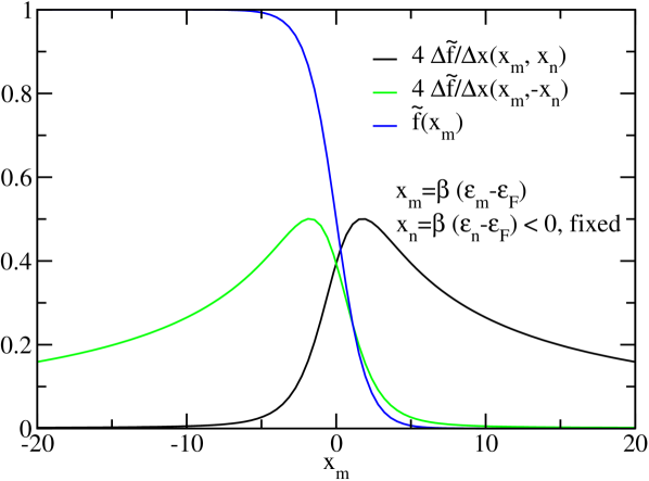
Figure 1: Behavior of Eq. (46) as a function of $x_{m}$ for a fixed negative value of $x_{n}$, ($x_{n}=-5$) and for $-x_{n}$. Note that those two plots are magnified by a factor of 4 for clarity. The Fermi-Dirac distribution $f(x_{m})$ as a function of the scaled variable $x_{m}$ also is shown.

In addition, the contributions of intra-band transitions and degenerate states make $S_{w}$ differ from unity. Only in the limits of large numbers of k-points, bands and a large frequency interval will $S_{w}\rightarrow 1$, if there are only non-degenerate inter-band contributions. If there are also intra-band or degenerate contributions, it will go to some value greater than one. However, the conductivity may reach convergence over the entire frequency interval of interest long before $S_{w}$ reaches convergence. Conversely, the value of $S_{w}$ could be around one or greater, depending on the afore-mentioned contributions, for a particular set of k-points and number of bands, but that does not mean that $S_{w}$ is converged and therefore that the conductivity is as well.

In consequence, convergence analysis with respect to the number of k-points and bands of the calculated conductivity itself over the frequency interval of interest is unavoidable.

3 Projector augmented wave method

Ordinarily the KS equations are solved by expanding the KS orbitals in a basis. A PW basis commonly is used both because the orbitals of simple metals resemble PWs and, more critically, because they are not centered on nuclear sites. Site-independence simplifies the use of KS DFT to drive ab initio molecular dynamics [14, 15, 16].

However, reproduction of the rapid oscillation of the KS orbitals near a nucleus would require an impracticably large PW basis. Conventionally that difficulty was alleviated by use of pseudo-potentials, but it was really solved, at least in principle, by the introduction of the PAW method [4]. Another significant advantage is that, distinct from pseudopotentials, the PAW approach allows for a significant simplification of the matrix elements of the operators while retaining the effect of core electrons.

The PAW method is based on the construction of a linear transformation which connects each KS orbital $|{\Psi}\rangle$ with a corresponding, much smoother pseudo-orbital $|{\tilde{\Psi}}\rangle$, that is

$$|{\Psi}\rangle=|{\tilde{\Psi}}\rangle+\sum_{i}\left[|{\phi_{i}}\rangle-|{\tilde{\phi_{i}}}\rangle\right]\langle{{\tilde{p_{i}}}}|{{\tilde{\Psi}}}\rangle\;.$$ (48)

The set $\{|{\phi}\rangle\}$ is an orthonormal basis, while the sets $\{|{\tilde{\phi}}\rangle\}$ and $\{|{\tilde{p}}\rangle\}$ form a dual basis. That is, besides the orthonormality and completeness conditions for the set $|{\phi}\rangle$s, one also has the duality conditions of completeness

$$\sum_{i}|{\tilde{\phi}_{i}}\rangle\langle{\tilde{p}_{i}}|=1$$ (49)

and orthonormality

$$\langle{\tilde{p}_{i}}|{\tilde{\phi}_{j}}\rangle=\delta_{ij},$$ (50)

between the other two sets. Physically, the set $\{|{\tilde{\phi}}\rangle\}$ is to be smoothed relative to the set $\{|{\phi}\rangle\}$, hence amenable to efficient plane-wave expansion.

The transformation connecting $|{\Psi}\rangle$ and $|{\tilde{\Psi}}\rangle$ is unitary and therefore any operator $A$ can be transformed to its smoothed version $\tilde{A}$ according to

$$\tilde{A}=A+\sum_{ij}|{\tilde{p_{i}}}\rangle(\langle{\phi_{i}}|A|{\phi_{j}}\rangle-\langle{\tilde{\phi}_{i}}|A|{\tilde{\phi}_{j}}\rangle)\langle{\tilde{p_{j}}}|.$$ (51)

In practice the $|{\phi_{i}}\rangle$s are taken as ground state atomic orbitals of a chemical element augmented with other eigenfunctions of the same Hamiltonian operator. The $|{\tilde{\phi}_{i}}\rangle$s are pseudized forms of the corresponding $|{\phi_{i}}\rangle$s. The $|{\tilde{p}_{i}}\rangle$s are defined as zero outside a sphere centered at the atom (augmentation sphere) and constructed to be the dual basis to the pseudized set inside the augmentation sphere. On the assumption that there is no overlap between augmentation spheres, the sum in Eq. (51) reduces from pairwise to a single atom. That is the so-called one-center approximation. It requires computational care to ensure negligible overlap of augmentation spheres in practice.

3.1 The $\langle{\Psi_{n\mathbf{k}}}|\nabla|{\Psi_{n^{\prime}\mathbf{k}}}\rangle$ matrix elements

Matrix elements of the velocity operator in the PAW representation follow from Eq. (51) as

$$\langle{\Psi_{n\mathbf{k}}}|\nabla|{\Psi_{n^{\prime}\mathbf{k}}}\rangle= \langle{\tilde{\Psi}_{n\mathbf{k}}}|\nabla|{\tilde{\Psi}_{n^{\prime}\mathbf{k}}}\rangle+$$

$$+\sum_{i}\sum_{\ell m}\sum_{\ell^{\prime}m^{\prime}}\langle{\tilde{\Psi}_{n\mathbf{k}}}|{\tilde{p}_{i\ell m}}\rangle\left[\langle{\varphi_{i\ell m}}|\nabla|{\varphi_{i\ell^{\prime}m^{\prime}}}\rangle-\langle{\tilde{\varphi}_{i\ell m}}|\nabla|{\tilde{\varphi}_{i\ell^{\prime}m^{\prime}}}\rangle\right]\langle{\tilde{p}_{i\ell^{\prime}m^{\prime}}}|{\tilde{\Psi}_{n^{\prime}\mathbf{k}}}\rangle,$$ (52)

with the atomic orbitals $|{\varphi_{i\ell m}}\rangle$, pseudo-orbitals $|{\tilde{\varphi}_{i\ell m}}\rangle$, and projectors $|{\tilde{p}_{i\ell m}}\rangle$ of atom $i$ (and associated augmentation region). Those are defined in terms of products of radial functions and spherical harmonics $Y_{\ell m}(\theta,\phi)$ (see  A) as

$$\varphi_{i\ell m}(\mathbf{r}-\mathbf{R}_{i})= R_{i\ell}(|\mathbf{r}-\mathbf{R}_{i}|)Y_{\ell m}(\theta,\phi),$$ (53)

$$\tilde{\varphi}_{ilm}(\mathbf{r}-\mathbf{R}_{i})= \tilde{R}_{i\ell}(|\mathbf{r}-\mathbf{R}_{i}|)Y_{\ell m}(\theta,\phi),$$ (54)

$$\tilde{p}_{i\ell m}(\mathbf{r}-\mathbf{R}_{i}) =\tilde{p}_{i\ell}(|\mathbf{r}-\mathbf{R}_{i}|)Y_{\ell m}(\theta,\phi)\;.$$ (55)

The one oddity (anticipating the practice in Quantum Espresso [3]) is that the principal quantum number is suppressed. One may think of the atom index $i$ as being a compound of site and principal quantum number. In compressed notation

$$\tilde{\nabla}_{nn^{\prime}}^{\mathbf{k}}\equiv \langle{\tilde{\Psi}_{n\mathbf{k}}}|\nabla|{\tilde{\Psi}_{n^{\prime}\mathbf{k}}}\rangle\;,$$ (56)

$$\gamma_{ilmn\mathbf{k}}^{\dagger}\equiv \langle{\tilde{\Psi}_{n\mathbf{k}}}|{\tilde{p}_{ilm}}\rangle\;,$$ (57)

$$\nabla_{ilml^{\prime}m^{\prime}}\equiv \langle{\varphi_{ilm}}|\nabla|{\varphi_{il^{\prime}m^{\prime}}}\rangle\;,$$ (58)

$$\tilde{\nabla}_{ilml^{\prime}m^{\prime}}\equiv \langle{\tilde{\varphi}_{ilm}}|\nabla|{\tilde{\varphi}_{il^{\prime}m^{\prime}}}\rangle\;,$$ (59)

Eq. (52) becomes

$$\nabla_{nn^{\prime}}^{\mathbf{k}}\equiv\langle{\Psi_{n\mathbf{k}}}|\nabla|{\Psi_{n^{\prime}\mathbf{k}}}\rangle=\tilde{\nabla}_{nn^{\prime}}^{\mathbf{k}}+\sum_{i}\sum_{lm}\sum_{l^{\prime}m^{\prime}}\gamma_{ilmn\mathbf{k}}^{\dagger}\left[\nabla_{ilml^{\prime}m^{\prime}}-\tilde{\nabla}_{ilml^{\prime}m^{\prime}}\right]\gamma_{il^{\prime}m^{\prime}n^{\prime}\mathbf{k}}\;.$$ (60)

The task is to find expressions for all the foregoing matrix elements.

It is straightforward to prove that

$$\tilde{\nabla}_{nn^{\prime}}^{\mathbf{k}}=i\sum_{\mathbf{G}}C_{n\mathbf{k}\mathbf{G}}^{*}\,C_{n^{\prime}\mathbf{k}\mathbf{G}}\,(\mathbf{k}+\mathbf{G});$$ (61)

For $\nabla_{i\ell m\ell^{\prime}m^{\prime}}$ we have

$$\nabla_{ilml^{\prime}m^{\prime}}= {\int}d^{3}r\,\varphi^{*}_{ilm}(\mathbf{r}-\mathbf{R}_{i})\nabla\varphi_{il^{\prime}m^{\prime}}(\mathbf{r}-\mathbf{R}_{i})$$

$$= {\int}d^{3}r\,\varphi^{*}_{ilm}(\mathbf{r})\nabla\varphi_{il^{\prime}m^{\prime}}(\mathbf{r})$$ (62)

where

$$\nabla\varphi_{il^{\prime}m^{\prime}}(\mathbf{r})= \frac{dR_{l^{\prime}}({r})}{dr}Y_{l^{\prime}m^{\prime}}(\theta,\varphi)\hat{\mathbf{e}}_{r}(\theta,\varphi)+\frac{R_{l^{\prime}}({r})}{r}\left[\frac{\partial Y_{l^{\prime}m^{\prime}}(\theta,\varphi)}{\partial\theta}\hat{\mathbf{e}}_{\theta}(\theta,\varphi)\right.$$

$$\left.+\frac{1}{\sin{\theta}}\frac{\partial Y_{l^{\prime}m^{\prime}}(\theta,\varphi)}{\partial\varphi}\ \hat{\mathbf{e}}_{\varphi}(\theta,\varphi)\right]\;.$$ (63)

Therefore,

$$\nabla_{ilml^{\prime}m^{\prime}}= \underbrace{\int_{0}^{\infty}r^{2}drR^{*}_{l}(r)\frac{dR_{l^{\prime}}({r})}{dr}}_{R^{(d)}_{ll^{\prime}}}\underbrace{\int_{0}^{\pi}\sin(\theta)d\theta\int_{0}^{2\pi}d\varphi Y^{*}_{lm}(\theta,\varphi)Y_{l^{\prime}m^{\prime}}(\theta,\varphi)\hat{\mathbf{e}}_{r}(\theta,\varphi)}_{=\mathbf{I}^{(r)}_{lml^{\prime}m^{\prime}}}$$

$$+ \underbrace{\int_{0}^{\infty}rdrR^{*}_{l}(r)R_{l^{\prime}}({r})}_{R_{ll^{\prime}}}\big{[}\underbrace{\int_{0}^{\pi}\sin(\theta)d\theta\int_{0}^{2\pi}d\varphi Y^{*}_{lm}(\theta,\varphi)\frac{\partial Y_{l^{\prime}m^{\prime}}(\theta,\varphi)}{\partial\theta}\hat{\mathbf{e}}_{\theta}(\theta,\varphi)}_{=\mathbf{I}^{(\theta)}_{lml^{\prime}m^{\prime}}}$$

$$+ \underbrace{\int_{0}^{\pi}d\theta\int_{0}^{2\pi}d\varphi Y^{*}_{lm}(\theta,\varphi)\frac{\partial Y_{l^{\prime}m^{\prime}}(\theta,\varphi)}{\partial\varphi}\hat{\mathbf{e}}_{\varphi}(\theta,\varphi)}_{=\mathbf{I}^{(\varphi)}_{lml^{\prime}m}}\big{]},$$ (64)

or

$$\nabla_{ilml^{\prime}m^{\prime}}= R^{(d)}_{ll^{\prime}}\mathbf{I}^{(r)}_{lml^{\prime}m^{\prime}}+R_{ll^{\prime}}\big{[}\mathbf{I}^{(\theta)}_{lml^{\prime}m}+\mathbf{I}^{(\varphi)}_{lml^{\prime}m^{\prime}})\big{]}.$$ (65)

The matrices $R^{d}$ and $R$ are calculated numerically while the vector matrices $\mathbf{I}$ are reduced to analytical forms ( B):

$$I^{(r)}_{lml^{\prime}m^{\prime},\hat{x}}= P^{(1)}_{lml^{\prime}m^{\prime}}A^{(c)}_{mm^{\prime}},$$ (66)

$$I^{(r)}_{lml^{\prime}m^{\prime},\hat{y}}= P^{(1)}_{lml^{\prime}m^{\prime}}A^{(s)}_{mm^{\prime}},$$ (67)

$$I^{(r)}_{lml^{\prime}m^{\prime},\hat{z}}= {P^{(2)}_{lml^{\prime}m^{\prime}}}\delta_{mm^{\prime}},$$ (68)

$$I^{(\theta)}_{lml^{\prime}m^{\prime},\hat{x}}= P^{(3)}_{lml^{\prime}m^{\prime}}{A^{(c)}_{mm^{\prime}}},$$ (69)

$$I^{(\theta)}_{lml^{\prime}m^{\prime},\hat{y}}= P^{(3)}_{lml^{\prime}m^{\prime}}{A^{(s)}_{mm^{\prime}}},$$ (70)

$$I^{(\theta)}_{lml^{\prime}m^{\prime},\hat{z}}= {P^{(4)}_{lml^{\prime}m^{\prime}}}\delta_{mm^{\prime}},$$ (71)

$$I^{(\varphi)}_{lml^{\prime}m^{\prime},\hat{x}}= -im^{\prime}{P^{(5)}_{lml^{\prime}m^{\prime}}}A^{(s)}_{mm^{\prime}},$$ (72)

$$I^{(\varphi)}_{lml^{\prime}m^{\prime},\hat{y}}= im^{\prime}{P^{(5)}_{lml^{\prime}m^{\prime}}}A^{(c)}_{mm^{\prime}}$$ (73)

and

$$I^{(\varphi)}_{lml^{\prime}m^{\prime},\hat{z}}=0\;.$$ (74)

The matrices $P^{(i)}(i=1...5)$ are developed in  C, while $A^{(c)}$ and $A^{(s)}$ are provided in  D.

Similarly for $\tilde{\nabla}_{ilml^{\prime}m^{\prime}}$ we have

$$\tilde{\nabla}_{ilml^{\prime}m^{\prime}}= \underbrace{\int_{0}^{\infty}r^{2}dr\tilde{R}^{*}_{l}(r)\frac{d\tilde{R}_{l^{\prime}}({r})}{dr}}_{\tilde{R}^{(d)}_{ll^{\prime}}}\underbrace{\int_{0}^{\pi}\sin(\theta)d\theta\int_{0}^{2\pi}d\varphi Y^{*}_{lm}(\theta,\varphi)Y_{l^{\prime}m^{\prime}}(\theta,\varphi)\hat{\mathbf{e}}_{r}(\theta,\varphi)}_{=\mathbf{I}^{(r)}_{lml^{\prime}m^{\prime}}}$$

$$+ \underbrace{\int_{0}^{\infty}rdr\tilde{R}^{*}_{l}(r)\tilde{R}_{l^{\prime}}({r})}_{\tilde{R}_{ll^{\prime}}}\big{[}\underbrace{\int_{0}^{\pi}\sin(\theta)d\theta\int_{0}^{2\pi}d\varphi Y^{*}_{lm}(\theta,\varphi)\frac{\partial Y_{l^{\prime}m^{\prime}}(\theta,\varphi)}{\partial\theta}\hat{\mathbf{e}}_{\theta}(\theta,\varphi)}_{={I}^{(\theta)}_{lml^{\prime}m^{\prime}}}$$

$$+ \underbrace{\int_{0}^{\pi}d\theta\int_{0}^{2\pi}d\varphi Y^{*}_{lm}(\theta,\varphi)\frac{\partial Y_{l^{\prime}m^{\prime}}(\theta,\varphi)}{\partial\varphi}\hat{\mathbf{e}}_{\varphi}(\theta,\varphi)}_{={I}^{(\varphi)}_{lml^{\prime}m^{\prime}}}\big{]},$$ (75)

or

$$\tilde{\nabla}_{ilml^{\prime}m^{\prime}}= \tilde{R}^{(d)}_{ll^{\prime}}\mathbf{I}^{(r)}_{lml^{\prime}m^{\prime}}+\tilde{R}_{ll^{\prime}}\big{[}\mathbf{I}^{(\theta)}_{lml^{\prime}m^{\prime}}+\mathbf{I}^{(\varphi)}_{lml^{\prime}m^{\prime}}\big{]}.$$ (76)

The formulae for the $\mathbf{I}$ integrals in terms of real spherical harmonics ( A) are given in  E (see also  D). The $P$ matrices are the same as for the complex spherical harmonics.

4 The KGEC code

4.1 Overview

On the foundations just laid, the KGEC code implements calculation of the full complex Kubo-Greenwood electrical conductivity tensor using the KS orbitals calculated by QE with either PAW datasets or norm-conserving pseudopotentials. (Note, however, that the latter case is without the non-local corrections.) KGEC is a post-processing tool for QE programmed in Fortran 90. It is modular and MPI-parallelized over k-points, bands, and plane waves. Details of parallelization are discussed below.

KGEC work flow is presented in Fig. 2. It presumes an ordinary QE calculation has been done which provides the KS orbitals, orbital energies, occupation numbers, temperature, and other relevant data via storage in the usual outdir directory. All that data is made accessible to KGEC by the QEVARS and QE_P_PSI modules.

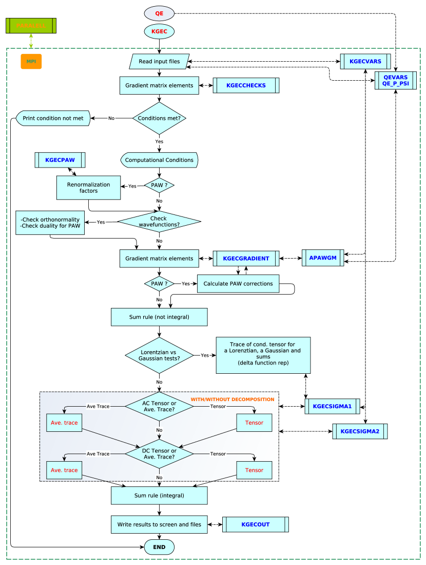
Figure 2: KGEC general work flow.

KGEC starts by reading an input file which provides the computational conditions for the conductivity calculation and the location of the QE data to use. It then verifies that the conditions for which the code was designed are met. If they are not, KGEC stops with a message about the problem and possible solutions, if discernible. Conversely, if the condition checks are satisfactory,the code proceeds to renormalize the PAW wave-functions (if PAWs are used) to avoid small errors in the normalization introduced by the construction of the PAW orbitals. Subsequently, if requested by the user, the code checks orthonormality and duality conditions for the pseudo-atomic orbitals and projectors (for PAWs).

Next comes calculation of the gradient matrix elements, via the KGEGRADIENT module, for pseudo-orbitals provided from QE and, if PAW datasets are utilized, a calculation of the PAW corrections is done via the APAWGM module of KGEC. Once the gradient matrix elements are completed, the sum rule without a delta function or frequency dependence (Eq. (41)) is calculated.

If selected by the user input, there follows the optional analysis of the effect of four different choices for numerical evaluation of the delta function (recall eq. 7), namely calculation of the average trace of the conductivity tensor done for a Lorentzian, a Gaussian, the sum of two Lorentzians, and the sum of two Gaussians (to eliminate problems at the origin).

Continuing, the code then proceeds to calculate either the full electrical conductivity tensor (including the average trace and the dc components), the average trace only (including the dc components), or the dc components only; all with or without decomposition. Those implementations are contained in the KGECSIGMA1 and KGECSIGMA2 modules. The sum rule for integration of the conductivity over frequencies (Eq. (43)) is calculated next.

Lastly, KGEC writes some additional information to the standard output and to the corresponding files.

4.2 MPI parallelization

In general KGEC is MPI-parallelized over k-points, bands, and plane waves via its PARALLEL module. That hierarchical order is the same as in QE. Parallelization over plane waves primarily is useful for gradient matrix element calculations. Once those matrix elements are done, the plane-wave-based parallelization is needless. However, the number of plane-waves greatly exceeds the number of bands. Usually that disparity is reflected in a larger number of processes used for plane waves than for bands. KGEC thus has the capacity to recover the MPI processes used for plane wave parallelization after gradient matrix element completion and add the recovered processes to the band parallelization processes.

More specifically KGEC is parallelized over k-points using the QE MPI communicator inter_pool_comm with $nk$ processes, over bands using the inter_bgrp_comm with $nb$ processes and over plane-waves using intra_bgrp_comm with $np$ processes. So, the total number of MPI processes is $nk\times nb\times np$. An example for 8 MPI processes is given in Table 1, with 2 processes dedicated to k-point parallelization, for each of them 2 dedicated to band parallelization, and for each of these 2 for plane-wave parallelization. Fig. 3 shows all the MPI processes and communicators in block form. With this scheme, the code can make those processes in the same communicator, i.e. those lying on the same blue rectangle in the figure, exchange information just by referencing their communicator. That allows for more efficient collective operations (scatter, gather,reduce), as well as code simplicity.

MPI Communicator	MPI Ranks								Parallelization
world_comm	0	1	2	3	4	5	6	7
inter_pool_comm	0	0	0	0	1	1	1	1	over k-points
inter_bgrp_comm	0	0	1	1	0	0	1	1	over bands
intra_bgrp_comm	0	1	0	1	0	1	0	1	over plane waves

Table 1: MPI communicators and each process rank for a parallelization over 8 processes, two for k points, two for bands, and two for plane waves.

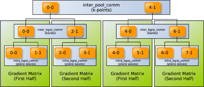
Figure 3: Block diagram of 8 MPI processes with two of them dedicated to k-point parallelization, two dedicated to band parallelization for each k-point process, and the other two dedicated for plane wave parallelization for each band process. A process is represented by a yellow rectangle, a communicator by a light-blue rectangle, the black lines connect the related processes in the parallel work flow, and the green rectangles represent the distribution of the gradient matrix. The first number in each process is its rank in the world_comm and the second is its rank in the communicator it belongs to or lies on.

Another key point is that the gradient matrix is distributed by the number of bands processes. Exact copies of those will end up stored in all the plane wave processes associated with the same band process. In other words, each process in an intra_bgrp_comm has exactly the same copy of a fragment of the gradient matrix that corresponds to the band process to which they are subordinated. In the specific case of Table 1, the gradient matrix is divided in halves, each of them residing on processes belonging to an inter_bgrp_comm value and replicated in the corresponding intra_bgrp_comm processes. That means that for the 0-0 branch of the k-point parallelization the same copy of the first half of the gradient matrix would be stored in the 0-0 and 1-1 processes, and the copy of the other half would be in the processes 2-0 and 3-1. A similar situation holds for the branch 4-1 of the k-point parallelization.

This structure is exploited for recovery of the plane wave processes that otherwise would be idle, hence wasted, after the calculation of gradient matrix elements, without any further communication.

Therefore, if the option to recover the plane wave processes is set to true (npwrecovery=.true.) then once the gradient matrix elements have been calculated, KGEC redefines the MPI communicators to use the plane wave processes for band parallelization. So, it goes from $nb$ band processes per k-point process to $nb\times np$ bands processes per k-point process, the gradient matrix elements being redistributed in place (without communication) between the $nb\times np$ bands processes. Coming back to the example of 8 MPI processes, the corresponding re-definition of the inter_bgrp_comm is given in Table 2 and the block diagram in Fig. 4. One sees that the band processes have expanded from 0 to 1 for each k-point process to 0,1,2,3. The half of the gradient matrix residing previously in each intra_bgrp_comm processes is divided by 2 and each bands process uses its own half from that point on. The rank 0 process in the previous intra_bgrp_comm keeps the first half and destroys the second one, while the rank 1 does the opposite. The final distribution is then one-quarter of the total columns of the gradient matrix per each process in the new inter_bgrp_comm.

MPI Communicator	MPI Ranks								Parallelization
world_comm	0	1	2	3	4	5	6	7
inter_pool_comm	0	0	0	0	1	1	1	1	over k-points
inter_bgrp_comm	0	1	2	3	0	1	2	3	over bands
intra_bgrp_comm	-	-	-	-	-	-	-	-	over plane waves

Table 2: MPI communicators and each process rank for a parallelization over 8 processes after recovery of the plane waves processes.

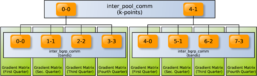
Figure 4: Block diagram of 8 MPI processes after recovery of the plane waves processes to be used for bands parallelization. There still are two processes dedicated to k-point parallelization, but four (instead of two as before) dedicated to band parallelization for each k-point process. A process is represented by a yellow rectangle, a communicator by a light-blue rectangle and the lines connect the related processes in the parallel work flow. The first number in each process is its rank in the world_comm and the second is its rank in the communicator it belongs to or lies on.

4.3 Prerequisites

The prerequisites for KGEC installation are:

• MPI for parallel compilation

• Fortran 90 compiler (Makefiles for Intel Linux Fortran provided ).

• Quantum Espresso 5.1.2, 5.2.1, 5.4.0, 6.0 or 6.1 installed for either serial or mpi-parallel execution or QE 5.2.1 compiled for use with Profess@QE [8].

(Remark: all of our installations have been in Linux with the Bourne-again shell.)

Both a README file and a more detailed User Guide are provided with the source code at download. They give installation instructions, along with instructions on how to do a simple example calculation. Input and reference output files for that calculation are provided. The example is fcc Aluminum with four atoms per unit cell at bulk density $\rho=2.7$ g/cm³ and temperature of 0.05 Rydberg (approximately 7,894 K). Note that if the example calculation (or any other for that matter) is run on more than one core, there will be differences with respect to the results from a serial calculation for the same input data. Such differences are the consequence of floating point arithmetic differences. However, as the number of k-points and bands are increased, the serial and parallel results should converge to the same values.

5 KGEC tests

5.1 Comparison with Abinit

We have calculated the average trace of the electrical conductivity using the approximated formula with two Gaussians (enforcing even parity of the conductivity) for Al fcc at bulk density $\rho=2.7$ g/cm³ and temperature $T=1$ eV for various numbers of k-points using KGEC and, for comparison, using Abinit. [17, 9, 18] The results are in very good agreement as Fig. 5 shows.

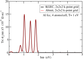
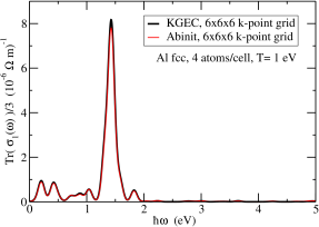
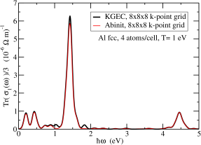
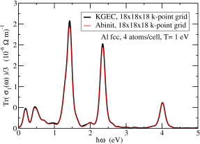
Figure 5: Comparison of KGEC and Abinit for different k-points in an ordered system; 4 atom/cell fcc Al at a density of 2.70 g/cm³.

However, for a more disordered system the results are sensitive to the k-point grid density. An example is for the ionic configuration from an arbitrarily selected molecular dynamics step of a 16 atom/cell Al system at $\rho=0.3$ g/cm³ and $10$ kK (about 0.86 eV). Results for the two codes differ for a $4\times 4\times 4$ k-point grid; see (Fig. 6). But comparison in Fig. 7 shows that the KGEC results are already converged at that grid density while those from Abinit are not.

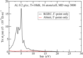
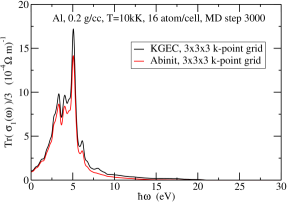
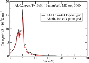
Figure 6: Comparison of KGEC and Abinit for different k-point grid densities in a disordered system: 16 atom/cell Al at an arbitrarily chosen MD step.

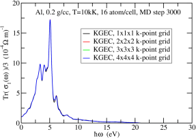
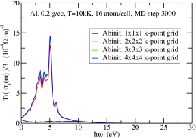
Figure 7: Convergence of KGEC (on the right) vs Abinit (on the left).

5.2 Consistency test

A consistency test also was performed by calculating the average of the conductivity for bcc Al with $2$ and $16$ atoms per unit cell at $\rho=0.2$ g/cm³ and $T=10$ kK. This low-density regime is of intrinsic physical interest [7]. Convergence with k-point grid density was reached for both systems at the $8\times 8\times 8$ grid, as can be seen in Fig. 8.

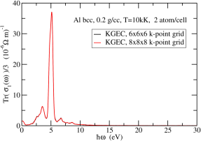
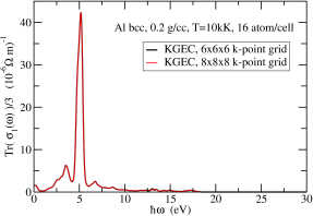
Figure 8: Convergence of KGEC for bcc Al with $2$ and $16$ atoms per unit cell at $\rho=0.2$ g/cm³ and $T=10$ kK.

However, comparison of the calculations for both systems performed with the $8\times 8\times 8$ mesh (Fig. 9) reveals that there are some discrepancies in the intensities of the highest peak and in the smaller peaks around $15$ eV in frequency. The changes are related to temperature and unit cell size effects. Notice however the very good agreement at low frequencies.

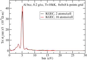
Figure 9: Comparison of the converged results for Al bcc $2$ and $16$ atoms per unit cell at $\rho=0.2$ g/cm³ and $T=10$ kK.

6 Difficulties

6.1 Representation of the Dirac delta function

It is frequent practice to use what we have called the “approximated expression”, Eq. (9), with a Gaussian representation for the Dirac delta function. Eq. (9) also can be written as

$$\sigma_{1}(\omega)=\frac{2\pi e^{2}\hbar^{2}}{m_{e}^{2}V}\sum_{m}\sum_{m^{\prime}}\frac{\Delta f_{m^{\prime}m}}{\Delta\epsilon_{mm^{\prime}}}\langle{m}|\nabla|{m^{\prime}}\rangle\langle{m^{\prime}}|\nabla|{m}\rangle\delta(\Delta\epsilon_{mm^{\prime}}-\hbar\omega),$$ (77)

denoted the as “Dirac-delta form” in the opening discussion. Observe that the main distinction between Eq. (9) and Eq. (77) is that the $\Delta\epsilon_{mm^{\prime}}$ in Eq. (77) is replaced by $\omega$ in Eq. (9).

We need to find the limits of Eq. (77) and Eq. (5) for $\omega$ going to zero in the cases in which a Lorentzian or a Gaussian (App. (F)) is used to represent the Dirac delta function. The issue reduces to evaluating four limits, to wit

$$\lim_{\omega\rightarrow 0}f^{(D-d)}_{L}(\omega)=\lim_{\omega\rightarrow 0}\frac{1}{\pi}\frac{\Delta f}{\Delta\epsilon}\frac{\delta/2}{(\Delta\epsilon-\hbar\omega)^{2}+\delta^{2}/4}=\frac{1}{\pi}\frac{\Delta f}{\Delta\epsilon}\frac{\delta/2}{(\Delta\epsilon)^{2}+\delta^{2}/4}$$ (78)

$$\lim_{\omega\rightarrow 0}f^{(D-d)}_{G}(\omega)=\lim_{\omega\rightarrow 0}\frac{\Delta f}{\Delta\epsilon}\frac{1}{\sigma_{g}\sqrt{\pi}}\;\exp{\left(-\frac{(\Delta\epsilon-\hbar\omega)^{2}}{\sigma^{2}_{g}}\right)}=\frac{\Delta f}{\Delta\epsilon}\frac{1}{\sigma_{g}\sqrt{\pi}}\;\exp{\left(-\frac{(\Delta\epsilon)^{2}}{\sigma^{2}_{g}}\right)}$$ (79)

$$\lim_{\omega\rightarrow 0}f^{(a)}_{L}(\omega)=\lim_{\omega\rightarrow 0}\frac{\Delta f}{\pi\omega}\frac{\delta/2}{(\Delta\epsilon-\hbar\omega)^{2}+\delta^{2}/4}=\pm\infty,$$ (80)

and

$$\lim_{\omega\rightarrow 0}f^{(a)}_{G}(\omega)=\lim_{\omega\rightarrow 0}\frac{\Delta f}{\omega}\frac{1}{\sigma_{g}\sqrt{\pi}}\;\exp{\left(-\frac{(\Delta\epsilon-\hbar\omega)^{2}}{\sigma^{2}_{g}}\right)}=\begin{cases}0&\exp(-(\Delta\epsilon)^{2})/\sigma_{g}^{2})=0\\ \pm\infty&\exp(-b(\Delta\epsilon)^{2}/\sigma_{g}^{2})\neq 0.\end{cases}$$ (81)

First notice that the approximated expressions, $f^{(a)}_{L}(\omega)$ and $f^{(a)}_{G}(\omega)$, do not have the same limit as the corresponding D-d expressions, $f^{(D-d)}_{L}(\omega)$ and $f^{(D-d)}_{G}(\omega)$. Instead, the approximated expressions are singular at $\omega=0$. Further, the two D-d versions $f^{(D-d)}_{L}(\omega)$ and $f^{(D-d)}_{G}(\omega)$ do not have the same limit, though they should be the same in the limit of the delta-width of the Lorentzian and the Gaussian going to zero.

The singularity of the approximated expressions can be lifted by using the even parity of $\sigma_{1}(\omega)$. In that case the limits are

$$\lim_{\omega\rightarrow 0}f^{(a)}_{L}(\omega)= \lim_{\omega\rightarrow 0}\frac{\Delta f}{2\pi\omega}\left(\frac{\delta/2}{(\Delta\epsilon-\hbar\omega)^{2}+\delta^{2}/4}-\frac{\delta/2}{(\Delta\epsilon+\hbar\omega)^{2}+\delta^{2}/4}\right)$$

$$= \frac{\delta\Delta f}{4\pi}\lim_{\omega\rightarrow 0}\frac{1}{\omega}\left(\frac{1}{(\Delta\epsilon-\hbar\omega)^{2}+\delta^{2}/4}-\frac{1}{(\Delta\epsilon+\hbar\omega)^{2}+\delta^{2}/4}\right)$$

$$= \frac{\delta\Delta f}{4\pi}\lim_{\omega\rightarrow 0}\frac{1}{\omega}\left(\frac{4\Delta\epsilon\hbar\omega}{((\Delta\epsilon-\hbar\omega)^{2}+\delta^{2}/4)((\Delta\epsilon+\hbar\omega)^{2}+\delta^{2}/4)}\right)$$

$$= \frac{\hbar}{\pi}{\delta\Delta f\,\Delta\epsilon}\lim_{\omega\rightarrow 0}\left(\frac{1}{((\Delta\epsilon-\hbar\omega)^{2}+\delta^{2}/4)((\Delta\epsilon+\hbar\omega)^{2}+\delta^{2}/4)}\right)$$

$$= \frac{\hbar}{\pi}\frac{\delta\Delta f\,\Delta\epsilon}{[(\Delta\epsilon)^{2}+\delta^{2}/4]^{2}},$$ (82)

and

$$\lim_{\omega\rightarrow 0}f^{(a)}_{G}(\omega)= \frac{\Delta f}{2\sigma_{g}\sqrt{\pi}}\;\lim_{\omega\rightarrow 0}\frac{1}{\omega}\left[\exp{\left(-\frac{(\Delta\epsilon-\hbar\omega)^{2}}{\sigma_{g}^{2}}\right)}-\exp{\left(-\frac{(\Delta\epsilon+\hbar\omega)^{2}}{\sigma_{g}^{2}}\right)}\right]$$

$$= \frac{2\hbar\Delta f\Delta\epsilon}{\sigma_{g}^{3}\sqrt{\pi}}\exp{\left(-\frac{(\Delta\epsilon)^{2}}{\sigma_{g}^{2}}\right)}\;.$$ (83)

But these limits are not the same as those in Eq. (78) and Eq. (79) either.

Just for completeness let us calculate the limit of the D-d expressions for the $f$s also taking into account the even parity of $\sigma_{1}$. For those we have

$$\lim_{\omega\rightarrow 0}f^{(D-d)}_{L}(\omega)= \frac{1}{2\pi}\frac{\Delta f}{\Delta\epsilon}\lim_{\omega\rightarrow 0}\left(\frac{\delta/2}{(\Delta\epsilon-\hbar\omega)^{2}+\delta^{2}/4}+\frac{\delta/2}{(\Delta\epsilon+\hbar\omega)^{2}+\delta^{2}/4}\right)$$

$$= \frac{1}{\pi}\frac{\Delta f}{\Delta\epsilon}\frac{\delta/2}{(\Delta\epsilon)^{2}+\delta^{2}/4},$$ (84)

and

$$\lim_{\omega\rightarrow 0}f^{(e)}_{G}(\omega)= \frac{\Delta f}{2\Delta\epsilon}\frac{1}{\sigma_{g}\sqrt{\pi}}\;\lim_{\omega\rightarrow 0}\left[\exp{\left(-\frac{(\Delta\epsilon-\hbar\omega)^{2}}{\sigma_{g}^{2}}\right)}+\exp{\left(-\frac{(\Delta\epsilon+\hbar\omega)^{2}}{\sigma_{g}^{2}}\right)}\right]$$

$$= \frac{\Delta f}{\Delta\epsilon}\frac{1}{\sigma_{g}\sqrt{\pi}}\;\exp{\left(-\frac{(\Delta\epsilon)^{2}}{\sigma_{g}^{2}}\right)},$$ (85)

results which are identical with Eq. (78) and Eq. (79).

The dc expressions then are

$$\sigma_{dc}^{D-d,L}=\frac{2e^{2}\hbar^{3}}{m_{e}^{2}V}\sum_{m}\sum_{m^{\prime}}\frac{\Delta f_{m^{\prime}m}}{\Delta\epsilon_{mm^{\prime}}}\langle{m}|\nabla|{m^{\prime}}\rangle\langle{m^{\prime}}|\nabla|{m}\rangle\frac{\delta/2}{(\Delta\epsilon_{mm^{\prime}})^{2}+\delta^{2}/4},$$ (86)

$$\sigma_{dc}^{D-d,G}=\frac{2\sqrt{\pi}e^{2}\hbar^{3}}{m_{e}^{2}V\sigma_{g}}\sum_{m}\sum_{m^{\prime}}\frac{\Delta f_{m^{\prime}m}}{\Delta\epsilon_{mm^{\prime}}}\langle{m}|\nabla|{m^{\prime}}\rangle\langle{m^{\prime}}|\nabla|{m}\rangle\;\exp{\left(-\frac{(\Delta\epsilon_{mm^{\prime}})^{2}}{\sigma_{g}^{2}}\right)},$$ (87)

$$\sigma_{dc}^{a,L}=\frac{4e^{2}\hbar^{3}}{m_{e}^{2}V}\sum_{m}\sum_{m^{\prime}}{\Delta f_{m^{\prime}m}}\Delta\epsilon_{mm^{\prime}}\langle{m}|\nabla|{m^{\prime}}\rangle\langle{m^{\prime}}|\nabla|{m}\rangle\frac{\delta/2}{((\Delta\epsilon_{mm^{\prime}})^{2}+\delta^{2}/4)^{2}},$$ (88)

and

$$\sigma_{dc}^{a,G}=\frac{4\sqrt{\pi}e^{2}\hbar^{3}}{m_{e}^{2}V\sigma_{g}^{3}}\sum_{m}\sum_{m^{\prime}}{\Delta f_{m^{\prime}m}}\Delta\epsilon_{mm^{\prime}}\langle{m}|\nabla|{m^{\prime}}\rangle\langle{m^{\prime}}|\nabla|{m}\rangle\;\exp{\left(-\frac{(\Delta\epsilon_{mm^{\prime}})^{2}}{\sigma_{g}^{2}}\right)}\;.$$ (89)

This simple analysis shows that in general the approximated $\sigma_{1}$ expressions Eq. (9) do not have correct low-frequency behavior, nor does the D-d form when evaluated with a Gaussian. Only the D-d expression with the Lorentzian recovers the exact limit of $\sigma_{1}$ for any value of the delta-width.

Numerical examples of the behavior of the $\sigma_{1}$ conductivity expressions are provided in two sets of figures. The first set (Fig. 10) shows results from calculations performed for fcc Al with four atoms per unit cell at a density of $2.7$ g/cm³ and a temperature of $31.6$ kK. To compare the effect of the Lorentzian versus Gaussian we did a set of calculations matching their full width at half-maximum (FWHM), and another matching their maximum heights.

As anticipated analytically, in general the approximated formulae lead to incorrect dc values, and also distort the spectra (peak shapes are changed) at low frequencies. The D-d formula with matched maximum heights for the Lorentzian and Gaussian leads to similar dc values, albeit with more distortion of the peak shape introduced by the Gaussian. Matching of the FWHM yields incorrect dc values but improves the line shapes for the Gaussian.

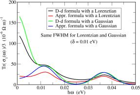
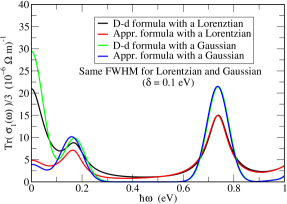
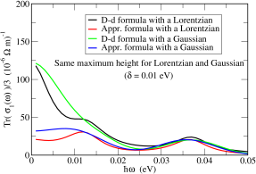
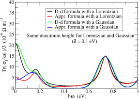
Figure 10: $Tr(\sigma_{1})/3$ calculated with approximations for the Dirac delta function for Al fcc with four atoms per unit cell density $=2.7$ g/cm³ and temperature $=31.6$ kK. The left column shows two figures for $\delta=0.01$ eV: the upper one shows results for the same FWHM for the Lorentzian and Gaussian representations, while the lower one is for the same maximum heights. The right column shows the same comparison for the case $\delta=0.1$ eV. In all panels the curves labeled “D-d formula …” show $Tr(\sigma_{1})/3$ calculated with Eq. (77) and curves labeled “Appr. formula …” show $Tr(\sigma_{1})/3$ calculated with Eq. (9).

The second set of figures (Fig. 11) shows calculations done for the ionic configuration from a molecular dynamics step of Al with 16 atoms per unit cell at 0.1 g/cm³ and a temperature of 30kK for 8 kps and 3096 bands. The panels are ordered the same way as in the preceding figure. In contrast with Fig. 10, they show that there are cases for which the delta function representations and width values are less important for the dc conductivity.

Another interesting aspect shown in Fig. 11 is that the smaller value of $\delta$ produces better convergence of all the delta function representations in the case of the MD step even when the spectrum gets noisier than the one calculated with a larger value of $\delta$.

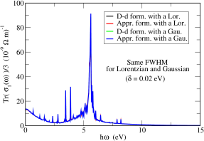
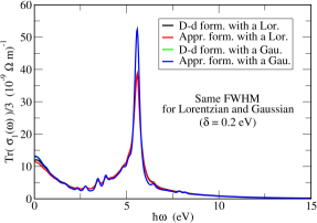
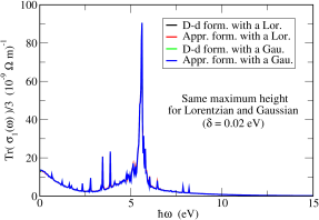
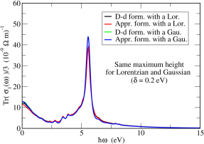
Figure 11: $Tr(\sigma_{1})/3$ calculated with different representations of the Dirac delta function for a molecular dynamics step of Al with $16$ atoms per unit cell at a density of $0.1$ g/cm³ and a temperature of $30$ kK. Otherwise as in Fig. 10.

Because of the relatively high temperature, in both cases the inter-band contributions dominate the dc conductivity and therefore the conductivity is not of Drude nature although the graphs look Lorentzian-like close to zero.

To get an idea of why the results are so different, we compare the cases of the D-d formula with the Lorentzian and the corresponding Gaussians with matching FWHM and maximum height. For that it will prove convenient to re-write the dc conductivity first in terms of one sum over bands by reducing the pair of $mm^{\prime}$ labels to one $i$-label, that is

$$\sigma_{dc}=\frac{2\pi e^{2}\hbar^{2}}{3m_{e}^{2}\Omega}\sum_{k}w_{\mathbf{k}}\sum_{i}\frac{\Delta f_{i\mathbf{k}}}{\Delta\epsilon_{i\mathbf{k}}}\sum_{\alpha}|\langle{\Psi_{m(i)\mathbf{k}}}|\nabla_{\alpha}|{\Psi_{m^{\prime}(i)\mathbf{k}}}\rangle|^{2}\delta(\Delta\epsilon_{i\mathbf{k}}),$$ (90)

and secondly by introducing $N(\Delta\epsilon_{j})$ as the number of pairs of states with the same difference in energy $\Delta\epsilon_{j}$ to get

$$\sigma_{dc}=\frac{2\pi e^{2}\hbar^{2}}{3m_{e}^{2}\Omega}\sum_{j}N(\Delta\epsilon_{j})\left[\sum_{\mathbf{k}}w_{\mathbf{k}}\sum_{i}\delta_{\Delta\epsilon_{i\mathbf{k}}\Delta\epsilon_{j}}\frac{\Delta f_{i\mathbf{k}}}{\Delta\epsilon_{i\mathbf{k}}}\sum_{\alpha}|\langle{\Psi_{m(i)\mathbf{k}}}|\nabla_{\alpha}|{\Psi_{m^{\prime}(i)\mathbf{k}}}\rangle|^{2}\right]\delta(\Delta\epsilon_{j}).$$ (91)

Plots of the three approximate representations of the Dirac delta function $\delta(\Delta\epsilon)$ and $N(\Delta\epsilon)$ for inter-band contributions (top), as well as their product (bottom), are given in Figures 12 and 13 for the respective examples given in Figures 10 and 11.

The sparsity of the $N(\Delta\epsilon)$ for fcc Al leads to functions with different areas when multiplied by the different delta function representations. In contrast, for the example from the MD step, the disorder is reflected in an almost uniform $N(\Delta\epsilon)$ which in turn yields distributions with almost the same area when multiplied with the approximate delta function representations. Therefore, it is the sparsity of the distribution of differences in energies $N(\Delta\epsilon)$ that seems to determine the success of the different delta-function representations in the dc conductivity calculation.

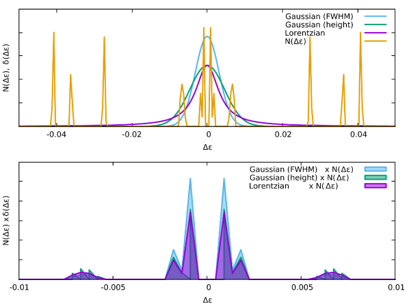
Figure 12: Dirac delta-function representations and number of pairs of bands with the same inter-band energy difference (top), and their product (bottom) for Al fcc with density of $2.7$ g/cm³ at T=$31.6$kK.

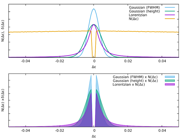
Figure 13: Dirac delta-function representations and number of pair of bands with the same inter-band energy difference (top), and their product (bottom) for a molecular dynamics step of Al at $0.1$ g/cm³ and T=$30$ kK.

6.2 PAW quality

During development of KGEC, we noticed some problems with the numerical derivatives involved in the calculation of the gradient matrix elements in the PAW approach. Close inspection of the radial atomic wave functions and pseudo-wave functions revealed that there seems to be a systematic problem in the generation of the augmented waves that is carried over to the corresponding pseudo-waves. The situation is represented in Fig. 14 for the atomic wave functions and in Fig. 15 for the pseudo wave functions generated for Al with three valence electrons and four projectors. Notice from Fig. 15 that the pseudo waves $\tilde{R}_{1}(r)$ and $\tilde{R}_{3}(r)$, generated from the $3s$ and $3p$ natural atomic states respectively, are smooth but $\tilde{R}_{2}(r)$ and $\tilde{R}_{4}(r)$, which were generated from the corresponding augmented-pseudized waves $\tilde{R}_{1}(r)$ and $\tilde{R}_{3}(r)$ respectively, are not.

The problem can be traced to the augmented waves themselves as corroborated by Fig. 14. We found the problem in four different PAW data sets generated with ATOMPAW [19] and LD1 [3]. This issue may need a bit more investigation, but it seems that the cancellation of errors that occurs in $\langle{R}|{dR/dr}\rangle-\langle{\tilde{R}}|{d\tilde{R}/dr}\rangle$ provides a way to get accurate results for properties calculated in the PAW scheme.

Another cancellation that occurs is in the product of the projectors and the pseudo-wave functions. That is given by the projectors being strictly zero starting at the radii where discontinuities in the first derivative of the pseudo wave functions appear and extending all the way to infinity. That should keep the dual orthogonality intact but it is not guaranteed, as illustrated by some tests described next.

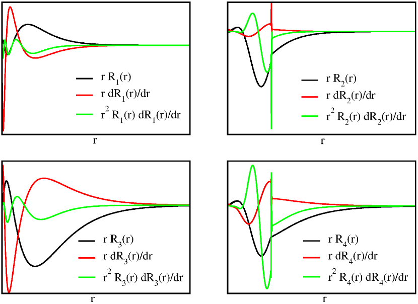
Figure 14: Atomic $3s$ ($R_{1}$ in the plot) and $3p$ ($R_{3}$ in the plot) wave functions of Al and their corresponding augmented waves ($R_{2}$ for $3s$ and $R_{4}$ for $3p$).

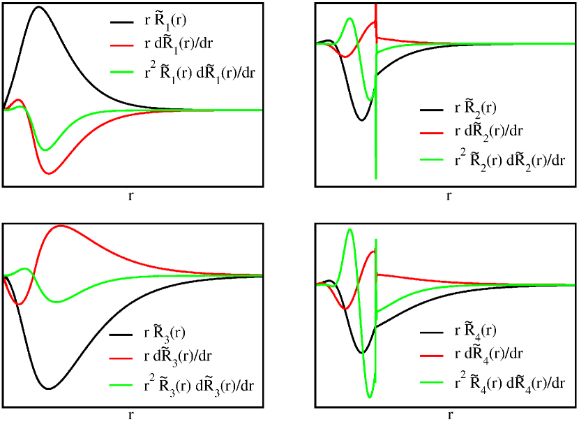
Figure 15: Atomic $3s$ ($\tilde{R}_{1}$ in the plot) and $3p$ ($\tilde{R}_{3}$ in the plot) pseudized wave functions of Al and their corresponding pseudized-augmented waves ($\tilde{R}_{2}$ for $3s$ and $\tilde{R}_{4}$ for $3p$).

6.3 PAW duality and wave functions orthogonality problems

Another difficulty observed during code development is related to the orthogonality required between pseudo-wavefunctions and projectors. Depending on the PAW dataset, there could be failures with errors larger than $10^{-4}$. That led to inclusion of a check for the dual orthogonality condition in KGEC.

There also are cases in which the reconstructed PAW all-electron orbitals are not orthogonal. This problem can be related to the dual orthogonality problem just described, but it can also arise from an inadequate plane wave basis set. KGEC is able to check for that sort of problem as well; it provides warnings and points the user to another output file for more information.

7 Remarks

From the perspective of a new computational implementation, we have reviewed the state of the art of electrical conductivity calculations using the Kubo Greenwood (KG) approach and derived all the necessary analytical expressions for its implementation using PAW data sets with a plane wave basis set. The analysis and derivations were done for both the original KG formula and it most popular version, which we have found contains approximations that often do not lead to the same results as the original one.

The derived formulae were used to design a user-friendly algorithm with capabilities to face the challenges of simulations of matter under extreme conditions. The algorithms have been coded in modular Fortran 90 as a post-processing tool for Quantum Espresso. Named KGEC, from the initials of “Kubo-Greenwood Electrical Conductivity”, the code has the following special features:

• Calculates the full complex conductivity tensor, not just the average trace.

• Uses either the original KG formula or the more popular, although approximated one in terms of a Dirac delta function.

• Performs a decomposition into intra- and inter-band contributions as well as degenerate state contributions.

• Calculates the direct-current conductivity tensor directly.

• Provides both Gaussian and Lorentzian representations of the Dirac delta function.

• Provides MPI parallelization over k-points, bands and plane waves, with an option to recover the plane waves process for their use in bands parallelization as well.

• Gives faster convergence with respect to k-point density than the implementation in the Abinit code.

KGEC is downloadable from http://www.qtp.ufl.edu/ofdft under GPL.

These features make the code versatile and innovative. There also are several underlying advances. An example is that the calculation of the direct-current tensor using the most popular KG formula is based on the removal of the singularity at zero frequency, an approach not reported before. That leads to analytical formulae, with the result that no fitting of a Drude term by the user is needed. Another example is the analysis which undergirds the systematic inclusion of both intra-band and degenerate state contributions in KGEC. A third example is the recovery of the plane waves MPI-processes on the fly, a procedure based on redefinition of the communicators and exploitation of MPI Single-Program-Multi-Data (SPMD) characteristics.

The code should have wide, deep impact on the calculation of electrical conductivities of materials ranging from small to large systems in normal to extreme environments. On one hand the possibility of doing full tensor calculations with no ballistic approximation should make the code attractive for the simulation of electronic materials. On the other, its parallel capabilities are very useful to accelerate simulations in general, but especially for large systems at high temperatures. For those, the plane wave cutoff energies and number of bands are very large, its parallel capabilities, including the recovery on the fly of idle processes, should make of KGEC an essential tool.

In the near future, the next release of our group’s Profess@QuantumEspresso [8] will include our new finite-temperature generalized gradient approximation (GGA)functional [20]. QE compiled for the Profess@QE suite is compatible with KGEC, so full free-energy DFT electrical conductivity calculations at the GGA level of refinement will be possible. Farther out, work within the context of electrical conductivity is likely to include incorporation of spin polarization, non-local corrections to the gradient matrix elements for systematic use of conventional non-local pseudopotentials, and inclusion of spin-orbit corrections. More broadly, we are considering generalizing to calculation of the thermal conductivity via general calculation of Onsager coefficients.

Appendix A Spherical harmonic definitions

The complex spherical harmonics are given by[21]

$$Y_{lm}(\theta,\varphi)=\sqrt{\frac{2l+1}{4\pi}}\sqrt{\frac{(l-m)!}{(l+m)!}}P_{l}^{m}(\cos\theta)e^{im\varphi}$$ (92)

with the sign conventions and definitions of the associated Legendre polynomials $P_{l}^{m}(x)$.

In the context of the PAW method it also is useful to use the real spherical harmonics, defined as

$$S_{lm}(\theta,\varphi)=\sqrt{\frac{2l+1}{4\pi}}\sqrt{\frac{(l-|m|)!}{(l+|m|)!}}P_{l}^{|m|}(\cos\theta)\begin{cases}\sqrt{2}\sin|m|\theta,&m<0\\ {1},&m=0\\ \sqrt{2}\cos m\theta,&{m>0}\end{cases}$$ (93)

Appendix B $I$ integrals for complex spherical harmonics

In the usual Cartesian coordinate system, the unit vectors relative to the spherical coordinates are

$$\hat{\mathbf{e}}_{r}= \sin(\theta)\cos(\varphi)\,\hat{\mathbf{e}}_{x}+\sin(\theta)\sin(\varphi)\,\hat{\mathbf{e}}_{y}+\cos(\varphi)\,\hat{\mathbf{e}}_{z}$$

$$\hat{\mathbf{e}}_{\theta}= \cos(\theta)\cos(\varphi)\,\hat{\mathbf{e}}_{x}+\cos(\theta)\sin(\varphi)\,\hat{\mathbf{e}}_{y}-\sin(\varphi)\,\hat{\mathbf{e}}_{z}$$

$$\hat{\mathbf{e}}_{\phi}= -\sin(\varphi)\,\hat{\mathbf{e}}_{x}+\cos(\varphi)\,\hat{\mathbf{e}}_{y}.$$ (94)

For $\mathbf{I}^{(r)}_{ll^{\prime}mm^{\prime}}$ we have

$$\mathbf{I}^{(r)}_{ll^{\prime}mm^{\prime}}={\int_{0}^{\pi}\sin(\theta)d\theta\int_{0}^{2\pi}d\varphi Y^{*}_{lm}(\theta,\varphi)Y_{l^{\prime}m^{\prime}}(\theta,\varphi)\hat{\mathbf{e}}_{r}(\theta,\varphi),}$$ (95)

which yields

$$I^{(r)}_{ll^{\prime}mm^{\prime},\hat{x}}= \int_{0}^{\pi}\sin(\theta)d\theta\int_{0}^{2\pi}d\varphi Y^{*}_{lm}(\theta,\varphi)Y_{l^{\prime}m^{\prime}}(\theta,\varphi)\sin(\theta)\cos(\varphi)$$

$$= C_{lm}C_{l^{\prime}m^{\prime}}\int_{0}^{\pi}\sin^{2}(\theta){P_{l}^{m}(\cos(\theta)}P_{l^{\prime}}^{m^{\prime}}(\cos(\theta))d\theta{\int_{0}^{2\pi}}\cos(\varphi)e^{i(m^{\prime}-m)\varphi}d\varphi$$

$$= \underbrace{2\pi C_{lm}C_{l^{\prime}m^{\prime}}\int_{-1}^{1}\sqrt{1-x^{2}}{P_{l}^{m}(x)}P_{l^{\prime}}^{m^{\prime}}(x)dx}_{P^{(1)}_{lml^{\prime}m^{\prime}}}\underbrace{\frac{1}{2\pi}\int_{0}^{2\pi}\cos(\varphi)e^{i(m^{\prime}-m)\varphi}d\varphi}_{A^{(c)}_{mm^{\prime}}}$$

$$= P^{(1)}_{lml^{\prime}m^{\prime}}A^{(c)}_{mm^{\prime}},$$ (96)

where

$$C_{lm}=\sqrt{\frac{2l+1}{4\pi}}\sqrt{\frac{(l-|m|)!}{(l+|m|)!}}\;.$$ (97)

Then

$$I^{(r)}_{ll^{\prime}mm^{\prime},\hat{y}}= {\int_{0}^{\pi}\sin(\theta)d\theta\int_{0}^{2\pi}d\varphi Y^{*}_{lm}(\theta,\varphi)Y_{l^{\prime}m^{\prime}}(\theta,\varphi)\sin(\theta)\sin(\varphi)}$$

$$= \underbrace{{2\pi C_{lm}C_{l^{\prime}m^{\prime}}}\int_{-1}^{1}\sqrt{1-x^{2}}{P_{l}^{m}(x)}P_{l^{\prime}}^{m^{\prime}}(x)dx}_{P^{(1)}_{lml^{\prime}m^{\prime}}}\underbrace{\frac{1}{2\pi}\int_{0}^{2\pi}\sin(\varphi)e^{i(m^{\prime}-m)\varphi}d\varphi}_{A^{(s)}_{mm^{\prime}}}$$

$$= P^{(1)}_{lml^{\prime}m^{\prime}}A^{(s)}_{mm^{\prime}};$$ (98)

$$I^{(r)}_{ll^{\prime}mm^{\prime},\hat{z}}= \int_{0}^{\pi}\sin(\theta)d\theta\int_{0}^{2\pi}d\varphi Y^{*}_{lm}(\theta,\varphi)Y_{l^{\prime}m^{\prime}}(\theta,\varphi)\cos(\theta)$$

$$= 2\pi C_{lm}C_{l^{\prime}m^{\prime}}\delta_{mm^{\prime}}\int_{0}^{\pi}\sin(\theta){P_{l}^{m}(\cos(\theta))}P_{l^{\prime}}^{m^{\prime}}(\cos(\theta))\cos(\theta)d\theta$$

$$= \underbrace{2\pi C_{lm}C_{l^{\prime}m^{\prime}}\int_{-1}^{1}x{P_{l}^{m}(x)}P_{l^{\prime}}^{m^{\prime}}(x)dx}_{P^{(2)}_{lml^{\prime}m^{\prime}}}\delta_{mm^{\prime}}$$

$$= {P^{(2)}_{lml^{\prime}m^{\prime}}}\delta_{mm^{\prime}};$$ (99)

For $\mathbf{I}^{(\theta)}_{ll^{\prime}mm^{\prime}}$ we have

$$\mathbf{I}^{(\theta)}_{ll^{\prime}mm^{\prime},\hat{x}}= \int_{0}^{\pi}\sin(\theta)d\theta\int_{0}^{2\pi}d\varphi Y^{*}_{lm}(\theta,\varphi)\frac{\partial Y_{l^{\prime}m^{\prime}}(\theta,\varphi)}{\partial\theta}\hat{\mathbf{e}}_{\theta}(\theta,\varphi),$$ (100)

which yields

$$I^{(\theta)}_{ll^{\prime}mm^{\prime},\hat{x}}= \int_{0}^{\pi}\sin(\theta)d\theta\int_{0}^{2\pi}d\varphi Y^{*}_{lm}(\theta,\varphi)\frac{\partial Y_{l^{\prime}m^{\prime}}(\theta,\varphi)}{\partial\theta}\cos(\theta)\cos(\varphi)$$

$$= 2\pi C_{lm}C_{l^{\prime}m^{\prime}}\int_{0}^{\pi}\sin(\theta){P_{l}^{m}(\cos(\theta))}\frac{\partial P_{l^{\prime}}(\cos(\theta))}{\partial\theta}\cos(\theta)d\theta\frac{1}{2\pi}\int_{0}^{2\pi}\cos(\varphi)e^{i(m^{\prime}-m)\varphi}d\varphi$$

$$= \underbrace{-2\pi C_{lm}C_{l^{\prime}}m^{\prime}\int_{-1}^{1}x\sqrt{1-x^{2}}{P_{l}^{m}(x)}\frac{dP_{l^{\prime}}^{m^{\prime}}(x)}{dx}dx}_{P^{(3)}_{lml^{\prime}m^{\prime}}}\underbrace{\frac{1}{2\pi}\int_{0}^{2\pi}\cos(\varphi)e^{i(m^{\prime}-m)\varphi}d\varphi}_{A^{(c)}_{mm^{\prime}}}$$

$$= P^{(3)}_{lml^{\prime}m^{\prime}}{A^{(c)}_{mm^{\prime}}};$$ (101)

$$I^{(\theta)}_{ll^{\prime}mm^{\prime},\hat{y}}= \int_{0}^{\pi}\sin(\theta)d\theta\int_{0}^{2\pi}d\varphi Y^{*}_{lm}(\theta,\varphi)\frac{\partial Y_{l^{\prime}m^{\prime}}(\theta,\varphi)}{\partial\theta}\cos(\theta)\sin(\varphi)$$

$$= \underbrace{-2\pi C_{lm}C_{l^{\prime}m^{\prime}}\int_{-1}^{1}x\sqrt{1-x^{2}}{P_{l}^{m}(x)}\frac{dP_{l^{\prime}}^{m^{\prime}}(x)}{dx}dx}_{P^{(3)}_{lml^{\prime}m^{\prime}}}\underbrace{\frac{1}{2\pi}\int_{0}^{2\pi}\sin(\varphi)e^{i(m^{\prime}-m)\varphi}d\varphi}_{A^{(s)}_{mm^{\prime}}}$$

$$= P^{(3)}_{lml^{\prime}m^{\prime}}{A^{(s)}_{mm^{\prime}}};$$ (102)

and

$$I^{(\theta)}_{ll^{\prime}mm^{\prime},\hat{z}}= \int_{0}^{\pi}\sin(\theta)d\theta\int_{0}^{2\pi}d\varphi Y^{*}_{lm}(\theta,\varphi)\frac{\partial Y_{l^{\prime}m^{\prime}}(\theta,\varphi)}{\partial\theta}(-\sin(\theta))$$

$$= 2\pi C_{lm}C_{l^{\prime}m^{\prime}}\delta_{mm^{\prime}}\int_{0}^{\pi}\sin(\theta){P_{l}^{m}(\cos(\theta))}\frac{\partial P_{l^{\prime}}^{m^{\prime}}(\cos(\theta))}{\partial\theta}(-\sin(\theta))d\theta$$

$$= \underbrace{-2\pi C_{lm}C_{l^{\prime}m^{\prime}}\int_{-1}^{1}(1-x^{2}){P_{l}^{m}(x)}\frac{dP_{l^{\prime}}^{m^{\prime}}(x)}{dx}dx}_{P^{(4)}_{lml^{\prime}m^{\prime}}}\delta_{mm^{\prime}}$$

$$= {P^{(4)}_{lml^{\prime}m^{\prime}}}\delta_{mm^{\prime}}.$$ (103)

For $\mathbf{I}^{(\varphi)}_{ll^{\prime}mm^{\prime}}$ we have

$$\mathbf{I}^{(\varphi)}_{ll^{\prime}mm^{\prime}}= \int_{0}^{\pi}d\theta\int_{0}^{2\pi}d\varphi Y^{*}_{lm}(\theta,\varphi)\frac{\partial Y_{l^{\prime}m^{\prime}}(\theta,\varphi)}{\partial\varphi}\hat{\mathbf{e}}_{\varphi}(\theta,\varphi)$$ (104)

which yields

$$I^{(\varphi)}_{ll^{\prime}mm^{\prime},\hat{x}}= \int_{0}^{\pi}d\theta\int_{0}^{2\pi}d\varphi Y^{*}_{lm}(\theta,\varphi)\frac{\partial Y_{l^{\prime}m^{\prime}}(\theta,\varphi)}{\partial\varphi}(-\sin(\varphi))$$

$$= 2\pi C_{lm}C_{l^{\prime}m^{\prime}}\int_{0}^{\pi}{P_{l}^{m}(\cos(\theta))}P_{l^{\prime}}^{m^{\prime}}(\cos(\theta))d\theta\frac{im^{\prime}}{2\pi}\int_{0}^{2\pi}(-\sin(\varphi)e^{i(m^{\prime}-m)\varphi})d\varphi$$

$$= \underbrace{2\pi C_{lm}C_{l^{\prime}m^{\prime}}\int_{-1}^{1}\frac{1}{\sqrt{1-x^{2}}}{P_{l}^{m}(x)}P_{l^{\prime}}^{m^{\prime}}(x)dx}_{P^{(5)}_{lml^{\prime}m^{\prime}}}\underbrace{\frac{im^{\prime}}{2\pi}\int_{0}^{2\pi}(-\sin(\varphi)e^{i(m^{\prime}-m)\varphi})d\varphi}_{-im^{\prime}A^{(s)}_{mm^{\prime}}}$$

$$= -im^{\prime}{P^{(5)}_{lml^{\prime}m^{\prime}}}A^{(s)}_{mm^{\prime}}$$ (105)

$$I^{(\varphi)}_{ll^{\prime}mm^{\prime},\hat{y}}= \int_{0}^{\pi}d\theta\int_{0}^{2\pi}d\varphi Y^{*}_{lm}(\theta,\varphi)\frac{\partial Y_{l^{\prime}m^{\prime}}(\theta,\varphi)}{\partial\varphi}\cos(\varphi)$$

$$= \underbrace{2\pi C_{lm}C_{l^{\prime}m^{\prime}}\int_{-1}^{1}\frac{1}{\sqrt{1-x^{2}}}{P_{l}^{m}(x)}P_{l^{\prime}}^{m^{\prime}}(x)dx}_{P^{(5)}_{lml^{\prime}m^{\prime}}}\underbrace{\frac{im^{\prime}}{2\pi}\int_{0}^{2\pi}\cos(\varphi)e^{i(m^{\prime}-m)\varphi}d\varphi}_{im^{\prime}A^{(c)}_{mm^{\prime}}}$$

$$= im^{\prime}{P^{(5)}_{lml^{\prime}m^{\prime}}}A^{(c)}_{mm^{\prime}};$$ (106)

and

$$I^{(\varphi)}_{ll^{\prime}mm^{\prime},\hat{z}}=0.$$ (107)

Appendix C Calculation of $P$ integrals

The $P$ integral general form is

$$P^{(1)}_{lml^{\prime}m^{\prime}}=2\pi C_{lm}C_{l^{\prime}m^{\prime}}\int_{-1}^{1}\sqrt{1-x^{2}}{P_{l}^{m}(x)}P_{l^{\prime}}^{m^{\prime}}(x)dx;$$ (108)

$$P^{(2)}_{lml^{\prime}m^{\prime}}=2\pi C_{lm}C_{l^{\prime}m^{\prime}}\int_{-1}^{1}x{P_{l}^{m}(x)}P_{l^{\prime}}^{m^{\prime}}(x)dx;$$ (109)

$$P^{(3)}_{lml^{\prime}m^{\prime}}=2\pi C_{lm}C_{l^{\prime}m^{\prime}}\int_{-1}^{1}x\sqrt{1-x^{2}}{P_{l}^{m}(x)}\frac{P_{l^{\prime}}^{m^{\prime}}(x)}{dx}dx;$$ (110)

$$P^{(4)}_{lml^{\prime}m^{\prime}}=-2\pi C_{lm}C_{l^{\prime}m^{\prime}}\int_{-1}^{1}(1-x^{2}){P_{l}^{m}(x)}\frac{dP_{l^{\prime}}^{m^{\prime}}(x)}{dx}dx;$$ (111)

and

$$P^{(5)}_{lml^{\prime}m^{\prime}}=2\pi C_{lm}C_{l^{\prime}m^{\prime}}\int_{-1}^{1}\frac{1}{\sqrt{1-x^{2}}}{P_{l}^{m}(x)}P_{l^{\prime}}^{m^{\prime}}(x)dx.$$ (112)

Each of these five matrices has $16$ by $16$ elements for $0\leq l\leq 3$. They were calculated symbolically using Maple.

Appendix D Calculation of $A$ integrals

The $A$ integrals for complex spherical harmonics are

$$A^{(c)}_{mm^{\prime}}= {\frac{1}{2\pi}\int_{0}^{2\pi}\cos(\varphi)e^{i(m^{\prime}-m)\varphi}d\varphi}$$

$$= \frac{1}{2}(\delta_{m+1,m^{\prime}}+\delta_{m-1,m^{\prime}}),$$ (113)

and

$$A^{(s)}_{mm^{\prime}}= {\frac{1}{2\pi}\int_{0}^{2\pi}\sin(\varphi)e^{i(m^{\prime}-m)\varphi}d\varphi}$$

$$= \frac{i}{2}(\delta_{m+1,m^{\prime}}-\delta_{m-1,m^{\prime}}).$$ (114)

For real spherical harmonics we have

$$A^{(c)}_{mm^{\prime}}= {\frac{1}{2\pi}\int_{0}^{2\pi}\cos(\varphi)\Phi_{m}(\varphi)\Phi_{m^{\prime}}(\varphi)d\varphi};$$ (115)

$$A^{(s)}_{mm^{\prime}}= {\frac{1}{2\pi}\int_{0}^{2\pi}\sin(\varphi)\Phi_{m}(\varphi)\Phi_{m^{\prime}}(\varphi)d\varphi};$$ (116)

$$A^{(c,d)}_{mm^{\prime}}= {\frac{1}{2\pi}\int_{0}^{2\pi}\cos(\varphi)\Phi_{m}(\varphi)\frac{\partial\Phi_{m^{\prime}}(\varphi)}{\partial\varphi}d\varphi};$$ (117)

and

$$A^{(s,d)}_{mm^{\prime}}= {\frac{1}{2\pi}\int_{0}^{2\pi}\sin(\varphi)\Phi_{m}(\varphi)\frac{\partial\Phi_{m^{\prime}}(\varphi)}{\partial\varphi}d\varphi}.$$ (118)

Appendix E $I$ integrals for real spherical harmonics

For $\mathbf{I}^{(r)}_{ll^{\prime}mm^{\prime}}$ we have

$$\mathbf{I}^{(r)}_{ll^{\prime}mm^{\prime}}={\int_{0}^{\pi}\sin(\theta)d\theta\int_{0}^{2\pi}d\varphi S_{lm}(\theta,\varphi)S_{l^{\prime}m^{\prime}}(\theta,\varphi)\hat{\mathbf{e}}_{r}(\theta,\varphi),}$$ (119)

which yields

$$I^{(r)}_{ll^{\prime}mm^{\prime},\hat{x}}= \int_{0}^{\pi}\sin(\theta)d\theta\int_{0}^{2\pi}d\varphi S_{lm}(\theta,\varphi)S_{l^{\prime}m^{\prime}}(\theta,\varphi)\sin(\theta)\cos(\varphi)$$

$$= C_{lm}C_{l^{\prime}m^{\prime}}\int_{0}^{\pi}\sin^{2}(\theta){P_{l}^{m}(\cos(\theta))}P_{l^{\prime}}^{m^{\prime}}(\cos(\theta))d\theta{\int_{0}^{2\pi}}\cos(\varphi)\Phi_{m}(\varphi)\Phi_{m^{\prime}}(\varphi)d\varphi$$

$$= \underbrace{2\pi C_{lm}C_{l^{\prime}m^{\prime}}\int_{-1}^{1}\sqrt{1-x^{2}}{P_{l}^{m}(x)}P_{l^{\prime}}^{m^{\prime}}(x)dx}_{P^{(1)}_{lml^{\prime}m^{\prime}}}\underbrace{\frac{1}{2\pi}\int_{0}^{2\pi}\cos(\varphi)\Phi_{m}(\varphi)\Phi_{m^{\prime}}(\varphi)d\varphi}_{A^{(c)}_{mm^{\prime}}}$$

$$= P^{(1)}_{lml^{\prime}m^{\prime}}A^{(c)}_{mm^{\prime}},$$ (120)

where we have used

$$\Phi_{m}(\varphi)=\begin{cases}\sqrt{2}\sin|m|\theta,&m<0\\ {1},&m=0\\ \sqrt{2}\cos m\theta,&{m>0}.\end{cases}$$ (121)

For the rest of the components of $\mathbf{I}^{(r)}_{ll^{\prime}mm^{\prime}}$ we have

$$I^{(r)}_{ll^{\prime}mm^{\prime},\hat{y}}= {\int_{0}^{\pi}\sin(\theta)d\theta\int_{0}^{2\pi}d\varphi S_{lm}(\theta,\varphi)S_{l^{\prime}m^{\prime}}(\theta,\varphi)\sin(\theta)\sin(\varphi)}$$

$$= \underbrace{{2\pi C_{lm}C_{l^{\prime}m^{\prime}}}\int_{-1}^{1}\sqrt{1-x^{2}}{P_{l}^{m}(x)}P_{l^{\prime}}^{m^{\prime}}(x)dx}_{P^{(1)}_{lml^{\prime}m^{\prime}}}\underbrace{\frac{1}{2\pi}\int_{0}^{2\pi}\sin(\varphi)\Phi_{m}(\varphi)\Phi_{m^{\prime}}(\varphi)d\varphi}_{A^{(s)}_{mm^{\prime}}}$$

$$= P^{(1)}_{lml^{\prime}m^{\prime}}A^{(s)}_{mm^{\prime}};$$ (122)

$$I^{(r)}_{ll^{\prime}mm^{\prime},\hat{z}}= \int_{0}^{\pi}\sin(\theta)d\theta\int_{0}^{2\pi}d\varphi S_{lm}(\theta,\varphi)S_{l^{\prime}m^{\prime}}(\theta,\varphi)\cos(\theta)$$

$$= 2\pi C_{lm}C_{l^{\prime}m^{\prime}}\delta_{mm^{\prime}}\int_{0}^{\pi}\sin(\theta){P_{l}^{m}(\cos(\theta))}P_{l^{\prime}}^{m^{\prime}}(\cos(\theta))\cos(\theta)d\theta$$

$$= \underbrace{2\pi C_{lm}C_{l^{\prime}m^{\prime}}\int_{-1}^{1}x{P_{l}^{m}(x)}P_{l^{\prime}}^{m^{\prime}}(x)dx}_{P^{(2)}_{lml^{\prime}m^{\prime}}}\delta_{mm^{\prime}}$$

$$= {P^{(2)}_{lml^{\prime}m^{\prime}}}\delta_{mm^{\prime}}.$$ (123)

For $\mathbf{I}^{(\theta)}_{ll^{\prime}mm^{\prime}}$ we have

$$\mathbf{I}^{(\theta)}_{ll^{\prime}mm^{\prime},\hat{x}}= \int_{0}^{\pi}\sin(\theta)d\theta\int_{0}^{2\pi}d\varphi S_{lm}(\theta,\varphi)\frac{\partial S_{l^{\prime}m^{\prime}}(\theta,\varphi)}{\partial\theta}\hat{\mathbf{e}}_{\theta}(\theta,\varphi),$$ (124)

which yields

$$I^{(\theta)}_{ll^{\prime}mm^{\prime},\hat{x}}= \int_{0}^{\pi}\sin(\theta)d\theta\int_{0}^{2\pi}d\varphi S_{lm}(\theta,\varphi)\frac{\partial S_{l^{\prime}m^{\prime}}(\theta,\varphi)}{\partial\theta}\cos(\theta)\cos(\varphi)$$

$$= 2\pi C_{lm}C_{l^{\prime}m^{\prime}}\int_{0}^{\pi}\sin(\theta){P_{l}^{m}(\cos(\theta))}\frac{\partial P_{l^{\prime}}(\cos(\theta))}{\partial\theta}\cos(\theta)d\theta\frac{1}{2\pi}\int_{0}^{2\pi}\cos(\varphi)\Phi_{m}(\varphi)\Phi_{m^{\prime}}(\varphi)d\varphi$$

$$= \underbrace{-2\pi C_{lm}C_{l^{\prime}}m^{\prime}\int_{-1}^{1}x\sqrt{1-x^{2}}{P_{l}^{m}(x)}\frac{dP_{l^{\prime}}^{m^{\prime}}(x)}{dx}dx}_{P^{(3)}_{lml^{\prime}m^{\prime}}}\underbrace{\frac{1}{2\pi}\int_{0}^{2\pi}\cos(\varphi)\Phi_{m}(\varphi)\Phi_{m^{\prime}}(\varphi)d\varphi}_{A^{(c)}_{mm^{\prime}}}$$

$$= P^{(3)}_{lml^{\prime}m^{\prime}}{A^{(c)}_{mm^{\prime}}};$$ (125)

$$I^{(\theta)}_{ll^{\prime}mm^{\prime},\hat{y}}= \int_{0}^{\pi}\sin(\theta)d\theta\int_{0}^{2\pi}d\varphi S_{lm}(\theta,\varphi)\frac{\partial S_{l^{\prime}m^{\prime}}(\theta,\varphi)}{\partial\theta}\cos(\theta)\sin(\varphi)$$

$$= \underbrace{-2\pi C_{lm}C_{l^{\prime}m^{\prime}}\int_{-1}^{1}x\sqrt{1-x^{2}}{P_{l}^{m}(x)}\frac{dP_{l^{\prime}}^{m^{\prime}}(x)}{dx}dx}_{P^{(3)}_{lml^{\prime}m^{\prime}}}\underbrace{\frac{1}{2\pi}\int_{0}^{2\pi}\sin(\varphi)\Phi_{m}(\varphi)\Phi_{m^{\prime}}(\varphi)d\varphi}_{A^{(s)}_{mm^{\prime}}}$$

$$= P^{(3)}_{lml^{\prime}m^{\prime}}{A^{(s)}_{mm^{\prime}}};$$ (126)

and

$$I^{(\theta)}_{ll^{\prime}mm^{\prime},\hat{z}}= \int_{0}^{\pi}\sin(\theta)d\theta\int_{0}^{2\pi}d\varphi S_{lm}(\theta,\varphi)\frac{\partial S_{l^{\prime}m^{\prime}}(\theta,\varphi)}{\partial\theta}(-\sin(\theta))$$

$$= 2\pi C_{lm}C_{l^{\prime}m^{\prime}}\delta_{mm^{\prime}}\int_{0}^{\pi}\sin(\theta){P_{l}^{m}(\cos(\theta))}\frac{\partial P_{l^{\prime}}^{m^{\prime}}(\cos(\theta))}{\partial\theta}(-\sin(\theta))d\theta$$

$$= \underbrace{-2\pi C_{lm}C_{l^{\prime}m^{\prime}}\int_{-1}^{1}(1-x^{2}){P_{l}^{m}(x)}\frac{dP_{l^{\prime}}^{m^{\prime}}(x)}{dx}dx}_{P^{(4)}_{lml^{\prime}m^{\prime}}}\delta_{mm^{\prime}}$$

$$= {P^{(4)}_{lml^{\prime}m^{\prime}}}\delta_{mm^{\prime}}.$$ (127)

For $\mathbf{I}^{(\varphi)}_{ll^{\prime}mm^{\prime}}$ we have

$$\mathbf{I}^{(\varphi)}_{ll^{\prime}mm^{\prime}}= \int_{0}^{\pi}d\theta\int_{0}^{2\pi}d\varphi S_{lm}(\theta,\varphi)\frac{\partial S_{l^{\prime}m^{\prime}}(\theta,\varphi)}{\partial\varphi}\hat{\mathbf{e}}_{\varphi}(\theta,\varphi)$$ (128)

which yields

$$I^{(\varphi)}_{ll^{\prime}mm^{\prime},\hat{x}}= \int_{0}^{\pi}d\theta\int_{0}^{2\pi}d\varphi S_{lm}(\theta,\varphi)\frac{\partial S_{l^{\prime}m^{\prime}}(\theta,\varphi)}{\partial\varphi}(-\sin(\varphi))$$

$$= 2\pi C_{lm}C_{l^{\prime}m^{\prime}}\int_{0}^{\pi}{P_{l}^{m}(\cos(\theta))}P_{l^{\prime}}^{m^{\prime}}(\cos(\theta))d\theta\frac{1}{2\pi}\int_{0}^{2\pi}(-\sin(\varphi))\Phi_{m}(\varphi)\frac{\partial\Phi_{m^{\prime}}(\varphi)}{\partial\varphi}d\varphi$$

$$= \underbrace{2\pi C_{lm}C_{l^{\prime}m^{\prime}}\int_{-1}^{1}\frac{1}{\sqrt{1-x^{2}}}{P_{l}^{m}(x)}P_{l^{\prime}}^{m^{\prime}}(x)dx}_{P^{(5)}_{lml^{\prime}m^{\prime}}}\underbrace{\frac{1}{2\pi}\int_{0}^{2\pi}(-\sin(\varphi))\Phi_{m}(\varphi)\frac{\partial\Phi_{m^{\prime}}(\varphi)}{\partial\varphi}d\varphi}_{-A^{(s,d)}_{mm^{\prime}}}$$

$$= -{P^{(5)}_{lml^{\prime}m^{\prime}}}A^{(s,d)}_{mm^{\prime}}$$ (129)

$$I^{(\varphi)}_{ll^{\prime}mm^{\prime},\hat{y}}= \int_{0}^{\pi}d\theta\int_{0}^{2\pi}d\varphi S_{lm}(\theta,\varphi)\frac{\partial S_{l^{\prime}m^{\prime}}(\theta,\varphi)}{\partial\varphi}\cos(\varphi)$$

$$= \underbrace{2\pi C_{lm}C_{l^{\prime}m^{\prime}}\int_{-1}^{1}\frac{1}{\sqrt{1-x^{2}}}{P_{l}^{m}(x)}P_{l^{\prime}}^{m^{\prime}}(x)dx}_{P^{(5)}_{lml^{\prime}m^{\prime}}}\underbrace{\frac{1}{2\pi}\int_{0}^{2\pi}\cos(\varphi)\Phi_{m}(\varphi)\frac{\partial\Phi_{m^{\prime}}(\varphi)}{\partial\varphi}d\varphi}_{A^{(c,d)}_{mm^{\prime}}}$$

$$= {P^{(5)}_{lml^{\prime}m^{\prime}}}A^{(c,d)}_{mm^{\prime}};$$ (130)

and

$$I^{(\varphi)}_{ll^{\prime}mm^{\prime},\hat{z}}=0.$$ (131)

Appendix F Lorentzian and Gaussian

The Lorentzian with a full width at half the maximum of $\delta$
has the expression

$$L(x)=\frac{1}{\pi}\frac{\delta/2}{x^{2}+{\delta^{2}}{/4}}$$ (132)

which equals half of its maximum amplitude for $x=\pm\delta/2$.

The Gaussian with width $\sigma_{g}$ is defined as

$$G(x)=\frac{1}{\sigma_{g}\sqrt{\pi}}\exp{\left(-\frac{x^{2}}{\sigma_{g}^{2}}\right)}.$$ (133)

Both functions are normalized to one. For the two to have the same height, the Gaussian width must be

$$\sigma_{g}=\frac{\delta}{2\sqrt{\pi}}\;,$$ (134)

while for equal FWHMs

$$\sigma_{g}=\frac{\delta}{2\sqrt{\ln{2}}}.$$ (135)

Appendix G References

References

• [1] Ryogo Kubo. Statistical-mechanical theory of irreversible processes. i. general theory and simple applications to magnetic and conduction problems. Journal of the Physical Society of Japan, 12(6):570–586, 1957.
• [2] D A Greenwood. The boltzmann equation in the theory of electrical conduction in metals. Proceedings of the Physical Society, 71(4):585, 1958.
• [3] Paolo Giannozzi, Stefano Baroni, Nicola Bonini, Matteo Calandra, Roberto Car, Carlo Cavazzoni, Davide Ceresoli, Guido L Chiarotti, Matteo Cococcioni, Ismaila Dabo, Andrea Dal Corso, Stefano de Gironcoli, Stefano Fabris, Guido Fratesi, Ralph Gebauer, Uwe Gerstmann, Christos Gougoussis, Anton Kokalj, Michele Lazzeri, Layla Martin-Samos, Nicola Marzari, Francesco Mauri, Riccardo Mazzarello, Stefano Paolini, Alfredo Pasquarello, Lorenzo Paulatto, Carlo Sbraccia, Sandro Scandolo, Gabriele Sclauzero, Ari P Seitsonen, Alexander Smogunov, Paolo Umari, and Renata M Wentzcovitch. Quantum espresso: a modular and open-source software project for quantum simulations of materials. Journal of Physics: Condensed Matter, 21(39):395502, 2009.
• [4] P. E. Blöchl. Projector augmented-wave method. Phys. Rev. B, 50:17953–17979, Dec 1994.
• [5] W. Kohn and L. J. Sham. Self-consistent equations including exchange and correlation effects. Phys. Rev., 140:A1133–A1138, Nov 1965.
• [6] Valentin V. Karasiev, Travis Sjostrom, James Dufty, and S. B. Trickey. Accurate homogeneous electron gas exchange-correlation free energy for local spin-density calculations. Phys. Rev. Lett., 112:076403, Feb 2014.
• [7] Valentin V. Karasiev, Lázaro Calderín, and S. B. Trickey. Importance of finite-temperature exchange-correlation for warm dense matter calculations. Phys. Rev. E, 93:063207, 2016.
• [8] Valentin V. Karasiev, Travis Sjostrom, and S. B. Trickey. Finite-temperature orbital-free dft molecular dynamics: Coupling profess and quantum espresso. Computer Physics Communications, 185(12):3240–3249, 2014.
• [9] X. Gonze, J.-M. Beuken, R. Caracas, F. Detraux, M. Fuchs, G.-M. Rignanese, L. Sindic, M. Verstraete, G. Zerah, F. Jollet, M. Torrent, A. Roy, M. Mikami, Ph. Ghosez, J.-Y. Raty, and D.C. Allan. First-principles computation of material properties: the abinit software project. Computational Materials Science, 25(3):478 – 492, 2002.
• [10] Stefano Baroni, Stefano de Gironcoli, Andrea Dal Corso, and Paolo Giannozzi. Phonons and related crystal properties from density-functional perturbation theory. Rev. Mod. Phys., 73:515–562, Jul 2001.
• [11] P.B. Allen. Conceptual foundations of materials: A standard model for ground- and excited-state properties. Contemporary Concepts of Condensed Matter Science, chapter 6. Elsevier Science, 2006.
• [12] Marco Cazzaniga, Lucia Caramella, Nicola Manini, and Giovanni Onida. Ab initio. Phys. Rev. B, 82:035104, Jul 2010.
• [13] P. Drude. Zur elektronentheorie der metalle. Annalen der Physik, 306(3):566–613, 1900.
• [14] D. Marx and J. Hutter. Ab initio molecular dynamics: Theory and implementation. In J. Grotendorst, editor, Modern Methods and Algorithms of Quantum Chemistry, pages 301–449. John von Neumann Institute for Computing (Jülich, NIC Series, Vol. 1 ), 2000.
• [15] J. S. Tse. Ab initio molecular dynamics with density functional theory. Annu. Rev. Phys. Chem., 53:249–290, 2002.
• [16] D. Marx and J. Hutter. Ab Initio Molecular Dynamics: Basic Theory and Advanced Methods. Cambridge University Press, 2009.
• [17] X. Gonze, B. Amadon, P.-M. Anglade, J.-M. Beuken, F. Bottin, P. Boulanger, F. Bruneval, D. Caliste, R. Caracas, M. Côté, T. Deutsch, L. Genovese, Ph. Ghosez, M. Giantomassi, S. Goedecker, D.R. Hamann, P. Hermet, F. Jollet, G. Jomard, S. Leroux, M. Mancini, S. Mazevet, M.J.T. Oliveira, G. Onida, Y. Pouillon, T. Rangel, G.-M. Rignanese, D. Sangalli, R. Shaltaf, M. Torrent, M.J. Verstraete, G. Zerah, and J.W. Zwanziger. Abinit: First-principles approach to material and nanosystem properties. Computer Physics Communications, 180(12):2582 – 2615, 2009. 40 YEARS OF CPC: A celebratory issue focused on quality software for high performance, grid and novel computing architectures.
• [18] Marc Torrent, François Jollet, François Bottin, Gilles Zèrah, and Xavier Gonze. Implementation of the projector augmented-wave method in the abinit code: Application to the study of iron under pressure. Computational Materials Science, 42(2):337 – 351, 2008.
• [19] N.A.W. Holzwarth, A.R. Tackett, and G.E. Matthews. A projector augmented wave (paw) code for electronic structure calculations, part i: atompaw for generating atom-centered functions. Computer Physics Communications, 135(3):329 – 347, 2001.
• [20] Valentin V. Karasiev, James W. Dufty, and S. B. Trickey. Nonempirical semi-local free-energy density functional for warm dense matter. arXiv, 1602:06266v2, 2016.
• [21] John David Jackson. Classical Electrodynamics. Wiley, New York, NY, 3rd edition, 1999.