Large scale quantum entanglement in de Sitter spacetime

Abstract

We investigate quantum entanglement between two symmetric spatial regions in de Sitter space with the Bunch-Davies vacuum. As a discretized model of the scalar field for numerical simulation, we consider a harmonic chain model. Using the coarse-grained variables for the scalar field, it is shown that the multipartite entanglement on the superhorizon scale exists by checking the monogamy relation for the negativity which quantifies the entanglement between the two regions. Further, we consider the continuous limit of this model without coarse-graining and find that non-zero values of the logarithmic negativity exist even if the distance between two spatial regions is larger than the Hubble horizon scale.

I Introduction

Quantum entanglement is an interesting aspect of quantum physics, which has recently received remarkable attention from various fields. As is well known in the quantum theory or quantum information theory, quantum entanglement represents a non-local correlation and leads to the violation of the Bell-CHSH inequality Bell1964b ; Clauser1969b . This quantum correlation is needed as a resource to carry out some protocols, e.g. quantum teleportation, superdense coding, quantum error correction and so on Nielsen2007 . For quantum many-body systems or quantum field theories, the entanglement of the ground state or vacuum state characterizes the structure of its wave function. In a previous work by S. Marcovitch et al. Marcovitch2009a , the quantum entanglement of a free Klein-Gordon field in the 1+1-dimensional Minkowski spacetime was examined in terms of the logarithmic negativity which is a useful measure to quantify the entanglement for a mixed state Vidal2002a . They focused on two spatially separated regions and numerically investigated the logarithmic negativity for the Minkowski vacuum as a function of the ratio of the separation between the regions to the size of the each region. It was shown that the logarithmic negativity decays exponentially as the ratio becomes large. This behavior is consistent with the Reeh-Schlieder theorem Reeh1961 which implies that the quantum entanglement persists for all scales for the Minkowski vacuum.

The nonlocal quantum correlation also was examined for cosmological situations Maldacena2015 ; Kanno2015 ; Kanno2014 ; Nambu2008 ; Nambu2011 . In a previous work by Y. Nambu Nambu2008 , the quantum entanglement of a massless scalar field in de Sitter space was investigated using the spatially coarse grained scalar field. It was revealed that the logarithmic negativity for the coarse-grained field vanishes, when the physical size of each region exceeds the Hubble horizon and becomes causally disconnected due to the de Sitter expansion. This behavior of entanglement is consistent with the scenario of quantum to classical transition of the primordial fluctuation generated by inflationary expansion in the early universe Guth1985 ; Polarski1996 ; Lesgourgues1997 ; Kiefer1998 ; Kiefer2007 ; Burgess2008 . The similar transition to zero negativity state is known for a model of 1+1-dimensional harmonic chain with a finite temperature Anders2008 . For sufficiently high temperatures, the negativity between two spatial regions becomes zero. Qualitatively, this transition can be understood as follows; above the critical temperature, the wavelength of the thermal fluctuations becomes shorter than the lattice spacing and the quantum correlation between adjacent lattice sites is destroyed by the thermal fluctuations. Concering the quantum field in de Sitter space, the effective comoving lattice spacing for the coarse-grained field becomes larger than the wavelength of quantum fluctuations which is equal to the Hubble length of de Sitter space, and the negativity becomes zero. We expect that appearance of zero negativity state is related to the coarse-graining treatment of the quantum field. As mentioned above, for the Minkowski vacuum in quantum field theory, the Reeh-Schrieder theorem is known and the theorem also holds for thermal states Jaekel2000 ; Narnhofer2005 . It seems that there is a difference between the feature of entanglement in the coarse-grained field and its continuous limit. Thus for complete understanding the property of the entanglement in de Sitter space, we need to analyze the quantum entanglement between two spatial regions using both a model with coarse-graining and one without coarse-graining.

In this paper, we use a 1+1-dimensional lattice model of a massless scalar field whose mode equation is equivalent to that of the 1+3-dimensional de Sitter spacetime and numerically evaluate the entanglement between two spatial regions. As a quantum state, we assume the Bunch-Davies vacuum, which is a vacuum state in de Sitter spacetime and corresponds to the Minkowski vacuum in the far remote past. We introduce coarse-grained variables in the lattice model and the negativity between two spatial regions is calculated. To understand the connection between the coarse-grained system and the continuous one, the effect of multipartite entanglement is considered using the monogamy relation for the negativity. We also compute the logarithmic negativity between the two regions without the coarse-graining and its behavior is discussed especially focusing on the continuous limit and the existence of the Hubble horizon.

This paper is organized as follows: we introduce our 1+1-dimensional lattice model of a minimal coupled massless scalar field in de Sitter spacetime and the entanglement measures (the negativity and the logarithmic negativity) for the Gaussian state in Sec. II. In Sec. III, we define the coarse-grained variables in the lattice system and calculate the negativity numerically. Then we discuss the monogamous property of the negativity. Also, we present our main numerical result of the logarithmic negativity without coarse-graining and provide the fitting formula for the super horizon scale. Sec. IV is devoted to summary and conclusion.

II Harmonic chain model and entanglement measures for Gaussian state

The Hamiltonian for a minimal coupled massless scalar field $q$ in de Sitter spacetime with a spatially flat slice is given by

$$\mathcal{H}=\int d^{3}x\frac{1}{2}\left[p^{2}+(\partial_{i}q)^{2}+\frac{1}{a}\frac{da}{d\eta}\,(qp+pq)\right],\quad a=-\frac{1}{H\eta},$$ (1)

where $a$ is the scale factor, $\eta<0$ is the conformal time and $H$ represents the Hubble constant. For simplicity of numerical analysis, we assume that the field depends only on the conformal time $\eta$ and one spatial coordinate. By introducing a lattice spacing $\Delta x$ of the spatial direction, the dimensionless form of the Hamiltonian of this model (harmonic chain) Nambu2008 is expressed as

$$\mathcal{H}=\sum_{j=1}^{N}\left[\frac{1}{2}\,p_{j}^{2}+q_{j}^{2}-\alpha\,q_{j}q_{j-1}+\frac{1}{2a}\frac{da}{d\tau}\,(p_{j}q_{j}+q_{j}p_{j})\right],$$ (2)

where we impose a periodic boundary condition on $q_{j}$ and $p_{j}$ to respect the translational invariance of the model. $N$ denotes the total number of lattice sites. $\tau$ and $\alpha$ are the dimensionless conformal time and the IR cutoff parameter, respectively. These two parameters are given by

$$\tau=\eta/\Delta x,\quad(m\Delta x)^{2}=2(1-\alpha),$$ (3)

where $m$ is the mass of the scalar field corresponding to the IR cutoff. We quantize this model as follows:

$$\hat{q}_{j}=\frac{1}{\sqrt{N}}\sum_{k=0}^{N-1}\left[\hat{a}_{k}\,f_{k}+\hat{a}_{N-k}^{\dagger}\,f_{k}^{*}\right]e^{i\theta_{k}j},\quad\hat{p}_{j}=\frac{-i}{\sqrt{N}}\sum_{k=0}^{N-1}\left[\hat{a}_{k}\,g_{k}-\hat{a}_{N-k}^{\dagger}\,g_{k}^{*}\right]e^{i\theta_{k}j},$$ (4)

where $\theta_{k}=2\pi k/N$. $\hat{a}_{k}$ and $\hat{a}_{k}^{\dagger}$ are annihilation and creation operators, which obey the commutation relations

$$\left[\hat{a}_{k},\hat{a}_{k^{\prime}}^{\dagger}\right]=\delta_{kk^{\prime}},\quad\left[\hat{a}_{k},\hat{a}_{k^{\prime}}\right]=\left[\hat{a}_{k}^{\dagger},\hat{a}_{k^{\prime}}^{\dagger}\right]=0.$$ (5)

The mode functions $f_{k}$ and $g_{k}$ satisfy

$$\ddot{f}_{k}+\left(\omega^{2}_{k}-\frac{\ddot{a}}{a}\right)f_{k}=0,\quad f_{k}\dot{f}^{*}_{k}-\dot{f}_{k}f^{*}_{k}=i,\quad g_{k}=i\left(\dot{f}_{k}-\frac{\dot{a}}{a}f_{k}\right),$$ (6)

where “$\cdot$” is the derivative with respect to $\tau$ and $\omega_{k}^{2}=2(1-\alpha\cos\theta_{k})$. Although this lattice model is introduced in the 1+1-dimensional spacetime, we assume that the equation of the mode functions has the same form as that in the 1+3-dimensional de Sitter space.

For the investigation of quantum entanglement of this system with the Bunch-Davies vacuum which belongs to a family of Gaussian states, we present a brief review of the negativity and the logarithmic negativity for a Gaussian state. Let us consider a phase space composed of canonical variables $\{\hat{q}_{j},\hat{p}_{j}\}_{j=1,...,N}$. The canonical commutation relations are

$$\left[\hat{R}_{j},\hat{R}_{k}\right]=i\Omega_{jk},\quad\Omega=\bigoplus_{j=1}^{N}J,\quad J=\begin{bmatrix}0&1\\ -1&0\end{bmatrix},$$ (7)

where $\hat{R}_{j}$ represent canonical variables defined by

$$\hat{R}=\left[\hat{q}_{1},\hat{p}_{1},...,\hat{q}_{N},\hat{p}_{N}\right]^{T}.$$ (8)

A Gaussian state $\hat{\rho}$ is determined by its first moment $\langle\hat{R}_{j}\rangle=\mathrm{Tr}[\hat{\rho}\,\hat{R}_{j}]$ and the covariance matrix

$$V_{jk}=\frac{1}{2}\,\mathrm{Tr}\left[\left(\Delta\hat{R}_{j}\,\Delta\hat{R}_{k}+\Delta\hat{R}_{k}\,\Delta\hat{R}_{j}\right)\hat{\rho}\right],\quad\Delta\hat{R}_{j}=\hat{R}_{j}-\langle\hat{R}_{j}\rangle.$$ (9)

The negativity $\mathcal{N}$ of a bipartite Gaussian state $\hat{\rho}_{AB}$ is given by using the symplectic eigenvalues of the partially transposed covariance matrix $\tilde{V}_{AB}$ Simon2000 obtained from $V_{AB}$ by replacing $\hat{p}_{jA}$ with $-\hat{p}_{jA}$ Marcovitch2009a :

$${\mathcal{N}}=\frac{1}{2}\Bigl{(}\prod_{j=1}^{N}\frac{1}{\min\left(2\tilde{\nu}_{j},1\right)}-1\Bigr{)},$$ (10)

where ${\tilde{\nu}}_{j}$ are positive eigenvalues of $i\,\Omega\,\tilde{V}_{AB}$. The sufficient condition for the entangled state is that the negativity $\mathcal{N}$ of the state does not vanish. The logarithmic negativity $E_{\mathcal{N}}$ is defined by the negativity as

$$E_{\mathcal{N}}=\ln\left[2{\mathcal{N}}+1\right].$$ (11)

The logarithmic negativity $E_{\mathcal{N}}$ provides an upper bound of the distillable entanglement (the number of the Bell pairs extractable from a bipartite state) Vidal2002a ; Plenio2005 , and if $E_{\mathcal{N}}$ is nonzero then the bipartite state is entangled. However, there exists an entangled state whose the entanglement of distillation vanishes and such a state is called a bound entangled state. Fortunately, no bound entangled state exists for a bipartite Gaussian state with $E_{\mathcal{N}}=0$ Giedke2001 .

To compute the negativity and the logarithmic negativity, we need the two-point functions of canonical variables on each site for the vacuum state. The correlation functions of the vacuum state are

$$\frac{1}{2}\langle 0|(\hat{q}_{j}\hat{q}_{l}+\hat{q}_{j}\hat{q}_{l})|0\rangle=\frac{1}{N}\sum_{k=0}^{N-1}|f_{k}|^{2}\cos\left[\theta_{k}(j-l)\right],$$ (12)

$$\frac{1}{2}\langle 0|(\hat{p}_{j}\hat{p}_{l}+\hat{p}_{l}\hat{p}_{j})|0\rangle=\frac{1}{N}\sum_{k=0}^{N-1}|g_{k}|^{2}\cos\left[\theta_{k}(j-l)\right],$$ (13)

$$\frac{1}{2}\langle 0|(\hat{q}_{j}\hat{p}_{l}+\hat{p}_{l}\hat{q}_{j})|0\rangle=\frac{1}{N}\sum_{k=0}^{N-1}\frac{i}{2}(f_{k}g^{*}_{k}-f^{*}_{k}g_{k})\cos\left[\theta_{k}(j-l)\right].$$ (14)

We choose the mode functions $f_{k}$ and $g_{k}$ which correspond to the Bunch-Davies vacuum as follows:

$$f_{k}=\frac{1}{\sqrt{2\omega_{k}}}\left(1+\frac{1}{i\omega_{k}\tau}\right)e^{-i\omega_{k}\tau},\quad g_{k}=\sqrt{\frac{\omega_{k}}{2}}\,e^{-i\omega_{k}\tau}.$$ (15)

In the continuous limit of the lattice model, the correlation functions of the Bunch-Davies vacuum are given as

$$\frac{1}{2}\langle 0|(\hat{q}(x,\eta)\hat{q}(y,\eta)+\hat{q}(y,\eta)\hat{q}(x,\eta))|0\rangle =\int^{\infty}_{-\infty}\frac{dk}{2\pi}|f_{k}|^{2}\cos[k(x-y)]$$

$$\sim\frac{1}{2\pi}(-\gamma-\ln[m|x-y|])+\frac{1}{2\pi(m\eta)^{2}},$$ (16)

$$\frac{1}{2}\langle 0|(\hat{p}(x,\eta)\hat{p}(y,\eta)+\hat{p}(y,\eta)\hat{p}(x,\eta))|0\rangle =\int^{\infty}_{-\infty}\frac{dk}{2\pi}|g_{k}|^{2}\cos[k(x-y)]$$

$$\sim-\frac{1}{2\pi|x-y|^{2}},$$ (17)

$$\frac{1}{2}\langle 0|(\hat{q}(x,\eta)\hat{p}(y,\eta)+\hat{p}(y,\eta)\hat{q}(x,\eta))|0\rangle =\int^{\infty}_{-\infty}\frac{dk}{2\pi}\frac{i}{2}(f_{k}g^{*}_{k}-f^{*}_{k}g_{k})\cos[k(x-y)]$$

$$\sim\frac{1}{2\pi\eta}(-\gamma-\ln[m|x-y|]),$$ (18)

where the above approximated formulas are obtained for $m|x-y|\ll 1$, and $\gamma$ is the Euler constant. The two-point correlation of our effective model in a 1+1-dimensional spacetime decrease with the distance $|x-y|$ more slowly compared to that in the 1+3-dimensional de Sitter space case.

III Behavior of entanglement

Because the scalar field is a many-body system, we expect that the multipartite entanglement is a key property to understand behavior of entanglement between two spatial regions in the de Sitter space. For this purpose, we introduce the coarse-grained field and the monogamy inequality of entanglement to quantify the multipartite entanglement of the scalar field.

III.1 Coarse-grained field and entanglement monogamy

To focus on the behavior of the multipartite entanglement, we introduce the coarse-grained variables $(\hat{Q}_{i},\hat{P}_{i})$ as follows:

$$\hat{Q}_{i}=\frac{1}{\sqrt{n_{\rm{c}}}}\sum_{j=0}^{n_{\rm{c}}-1}\hat{q}_{n_{\rm{c}}i+j},~{}\hat{P}_{i}=\frac{1}{\sqrt{n_{\rm{c}}}}\sum_{j=0}^{n_{\rm{c}}-1}\hat{p}_{n_{\rm{c}}i+j},$$ (19)

where we denote $n_{\rm{c}}$ as the coarse-graining size of the canonical variables. The coarse-grained variables satisfy the canonical commutation relations

$$\Bigl{[}\hat{Q}_{i},~{}\hat{P}_{j}\Bigr{]}=i\delta_{ij},~{}\Bigl{[}\hat{Q}_{i},~{}\hat{Q}_{j}\Bigr{]}=\Bigl{[}\hat{P}_{i},~{}\hat{P}_{j}\Bigr{]}=0.$$ (20)

We introduce two spatial symmetric regions A and B by choosing the following coarse-grained variables in the harmonic chain:

$$\hat{R}^{A}=\left[\hat{Q}_{1},\hat{P}_{1},...,\hat{Q}_{n},\hat{P}_{n}\right]^{T},~{}\hat{R}^{B}=\left[\hat{Q}_{n+1+d/n_{\rm{c}}},\hat{P}_{n+1+d/n_{\rm{c}}},...,\hat{Q}_{2n+d/n_{\rm{c}}},\hat{P}_{2n+d/n_{\rm{c}}}\right]^{T}$$ (21)

where $n$ is the number of modes of the coarse-grained variables contained in each region, and $d$ is the comoving separation between A and B. The comoving size of each region is denoted as $l=n\times n_{\rm{c}}$ (FIG. 1).

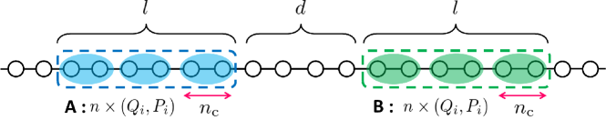
Figure 1: Two spatial symmetric regions A and B in the harmonic chain. $l$ is the comoving size of each region and $d$ is the comoving distance between the two regions. $n_{\rm{c}}$ is the coarse-graining size for each system and $n$ are the number of modes of the coarse-grained variables included in each region.

Since the vacuum state is Gaussian, the quantum bipartite entanglement can be completely characterized by the covariance matrix defined as

$$V_{AB}=\begin{bmatrix}A&C\\ C^{T}&B\end{bmatrix},\quad A^{T}=A,\quad B^{T}=B$$ (22)

where $A,B,C$ are $2n\times 2n$ matrices given by

$$A_{ij}=\frac{1}{2}\langle 0|\bigl{(}\hat{R}^{A}_{i}\hat{R}^{A}_{j}+\hat{R}^{A}_{j}\hat{R}^{A}_{i}\bigr{)}|0\rangle,$$

$$B_{ij}=\frac{1}{2}\langle 0|\bigl{(}\hat{R}^{B}_{i}\hat{R}^{B}_{j}+\hat{R}^{B}_{j}\hat{R}^{B}_{i}\bigr{)}|0\rangle,$$

$$C_{ij}=\frac{1}{2}\langle 0|\bigl{(}\hat{R}^{A}_{i}\hat{R}^{B}_{j}+\hat{R}^{B}_{j}\hat{R}^{A}_{i}\bigr{)}|0\rangle,$$ (23)

with $\langle 0|\hat{R}_{i}^{(A,B)}|0\rangle=0$. In Ref. Nambu2008 , the logarithmic negativity between A and B were calculated with the number of each mode $n=1$, which corresponds to assigning a pair of canonical variables to each region.

The following results are based on the numerical calculation with the number of lattice sites $N=2\times 10^{4}$ and the IR cutoff parameter $\alpha=1-10^{-12}$. FIG. 2 shows behavior of the negativity with different size of coarse-graining. The left panel of FIG. 2 presents the time evolution of the negativity with fixed the comoving distance $d=0$ and the comoving size $l=60$. As the number of modes of the coarse-grained variables $n$ in the system A increases, the time at which the negativity vanishes becomes later. The right panel of FIG. 2 gives the distance dependence of the negativity with fixed $l=60$ and $\tau=-80$. For a larger $n$, the negativity increases and vanishes at a larger distance $d$.

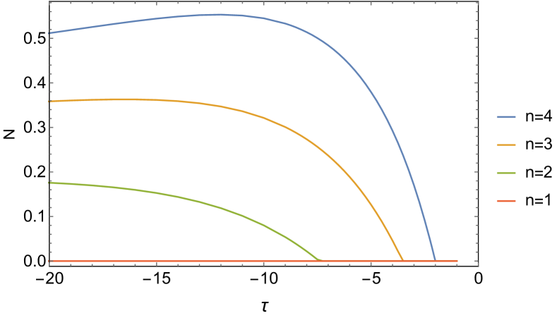
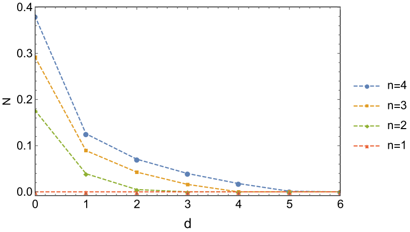
Figure 2: The negativity with different size of the coarse-graining . The left panel: the negativity ${\mathcal{N}}$ as a function of $\tau$ with $d=0$ and $l=60$. The right panel: the negativity ${\mathcal{N}}$ as a function of $d$ for $\tau=-80$.

To compare the previous work Nambu2008 with our results, we introduce

$$l_{p}=-l/\tau,\quad d_{p}=-d/\tau,$$ (24)

where $l_{p}$ and $d_{p}$ represent the proper (physical) size of each region and the distance between the two regions in the unit of the Hubble length $H^{-1}$, respectively. In Ref. Nambu2008 , it is found that the quantum entanglement between A and B with the number of each mode $n=1$ disappears when the proper size of each region is comparable to the Hubble horizon, that is, at $l_{\rm{p}}=1$. This means that the quantum fluctuation for the super horizon scale behaves classically in terms of bipartite entanglement. However, according to the left panel of FIG. 2, we find that the quantum entanglement with the number of each mode $n\geq 2$ in the system A and B does not vanish even if the proper size of each region $l_{\rm{p}}$ is larger than $1$ (for example, in the case $n=2$, the negativity is nonzero at $\tau=-10,l=60$, that is, $l_{\rm{p}}=6$) . Hence we expect there exists the multipartite entanglement even for the quantum fluctuation in the super horizon scale. Also, in the right panel of FIG. 2, the maximum distance that the negativity exists increases monotonically as $n$ increases (in Ref. Nambu2008 , the negativity vanishes trivially for $d\geq 1$). It seems that the multipartite entanglement between casually disconnected regions also survives for a larger $n$ (in the following section B, we clarify the distance dependence for the continuous limit of our model).

To get a clear intuition for the behavior of FIG. 2, we introduce the monogamy relation of the negativity for this model. We consider a tripartite state $\rho_{ABC}$ and the negativity ${\mathcal{N}}_{AB|C}$ between AB and C. It is conjectured that ${\mathcal{N}}_{A|C},{\mathcal{N}}_{B|C}$ and ${\mathcal{N}}_{AB|C}$ obeys the following inequality

$${\mathcal{N}}^{2}_{AB|C}\geq{\mathcal{N}}^{2}_{A|C}+{\mathcal{N}}_{B|C}^{2},$$ (25)

where ${\mathcal{N}}_{A|C}$ and ${\mathcal{N}}_{B|C}$ are the negativity between AC or BC, respectively. This is called the monogamy relation of the negativity, which is an crucial property of the quantum entanglement. The monogamy relation is proved for a multi-qubit system Osborn2006 , and the similar relation holds for the entanglement measure defined in the Gaussian system Hiroshima2007 . However, there is no proof of the monogamy relation of the negativity for the Gaussian system. If the monogamy relation holds then the multipartite entanglement can be expressed by the quantity

$${\mathcal{N}}_{A|B|C}:={\mathcal{N}}^{2}_{AB|C}-{\mathcal{N}}^{2}_{A|C}-{\mathcal{N}}_{B|C}^{2}.$$ (26)

This is the difference between the two side of Eq. (25) and can be interpreted as the residual entanglement. If this quantity vanishes, the entanglement between AB and C can be decomposed to the entanglement between A and C, and the entanglement between B and C. Thus the entanglement between AB and C is written as sum of pure bipartite entanglement between sub system. In such a case, there is no multipartite entanglement.

To understand the multipartite entanglement in the Bunch-Davies vacuum, we consider the negativity with the number of each mode $n=3$ in the systems A and B (FIG. 3). The density operator $\hat{\rho}_{AB}$ is a $3\times 3$ mode Gaussian state and the system A is composed of $3$ subsystems $\rm{A_{1}A_{2}A_{3}}$ (similarly, B is $\rm{B_{1}B_{2}B_{3}}$). The monogamy relation is written as

$${\mathcal{N}}^{2}_{A^{\otimes 3}|B}\geq{\mathcal{N}}_{A^{\otimes 2}|B}^{2}+{\mathcal{N}}^{2}_{A^{\otimes 1}|B},$$ (27)

where $A^{\otimes 3}=A_{1}A_{2}A_{3}$ and $(A^{\otimes 2},A^{\otimes 1})=(A_{1}A_{2},A_{3}),~{}(A_{1}A_{3},A_{2}),~{}(A_{2}A_{3},A_{1})$. For example, each negativity ${\mathcal{N}}_{A_{2}A_{3}|B},~{}{\mathcal{N}}_{A_{1}A_{3}|B}$ and ${\mathcal{N}}_{A_{3}|B}$ which appears on the right side for (27) corresponds to the entanglement between the two regions A and B shown in FIG. 3.

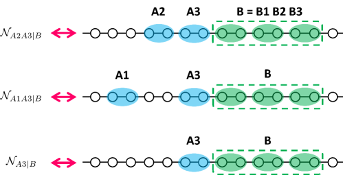
Figure 3: The correspondence between each negativity in the tripartite system and the two regions AB for $d=0$.

Let us check the monogamy relation of the negativity for the Bunch-Davies vacuum in the case $n=3$. The left and right panel of FIG. 4 present the time dependence with $d=0$ and the distance dependence at $\tau=-80$ of the quantity ${\mathcal{N}}_{A^{\otimes 2}|A^{\otimes 1}|B}$, respectively.

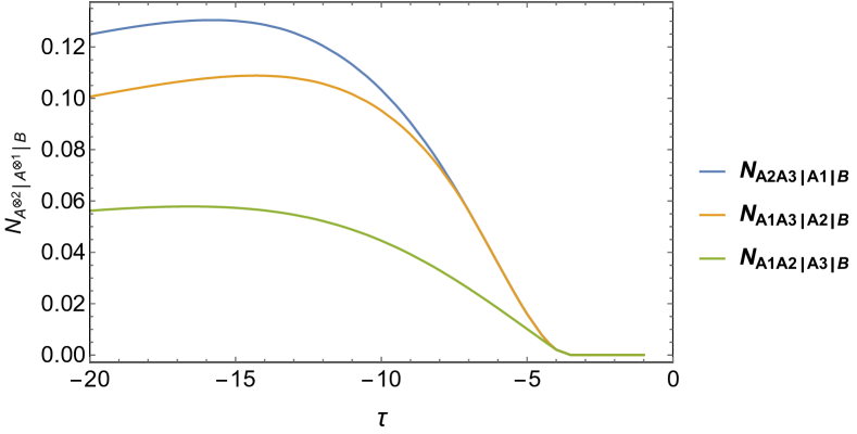
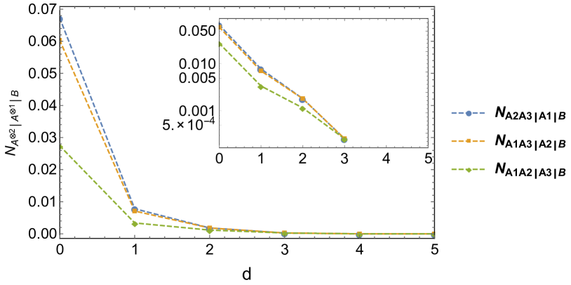
Figure 4: Left panel: the time dependence of ${\mathcal{N}}_{A^{\otimes 2}|A^{\otimes 1}|B}$ with $d=0$. Right panel: the distance dependence of ${\mathcal{N}}_{A^{\otimes 2}|A^{\otimes 1}|B}$ at $\tau=-80$

From these results, we confirm that the monogamous relation of the negativity ${\mathcal{N}}_{A^{\otimes 2}|A^{\otimes 1}|B}\geq 0$ holds for our model. Hence we can characterize the multipartite entanglement in de Sitter space by the negativity.

In the left panel of FIG. 5, the time dependence of ${\mathcal{N}}^{2}_{A_{1}A_{2}A_{3}|B},~{}{\mathcal{N}}^{2}_{A_{2}A_{3}|B},~{}{\mathcal{N}}^{2}_{A_{1}A_{3}|B}$ and ${\mathcal{N}}^{2}_{A_{3}|B}$ for $d=0$ is shown (the other cases ${\mathcal{N}}_{A_{1}A_{2}|B},~{}{\mathcal{N}}_{A_{1}|B}$ and ${\mathcal{N}}_{A_{2}|B}$ are trivially zero). We observe that the negativities ${\mathcal{N}}^{2}_{A^{\otimes 1}|B}$ and ${\mathcal{N}}^{2}_{A^{\otimes 2}|B}$ decay faster than the negativity ${\mathcal{N}}^{2}_{A^{\otimes 3}|B}$ for the $3\times 3$ mode Gaussian system. This behavior guarantees the monogamy inequality (25).

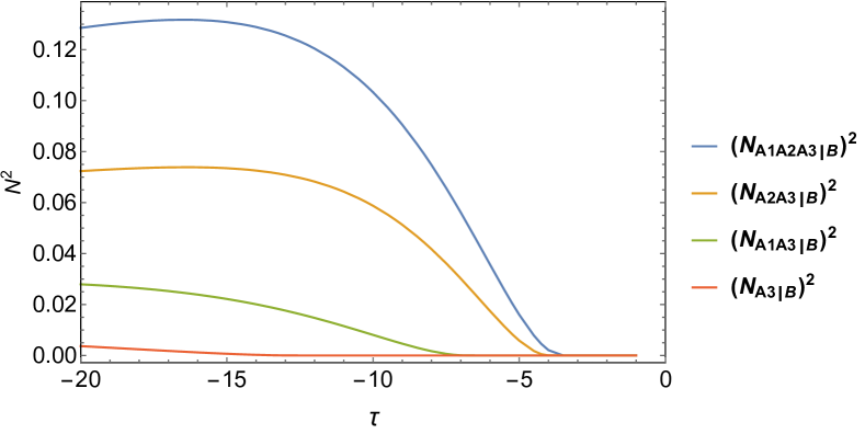
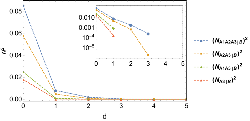
Figure 5: Left panel: square of each negativity ${\mathcal{N}}_{A_{2}A_{3}|B},~{}{\mathcal{N}}_{A_{1}A_{3}|B}$ and ${\mathcal{N}}_{A_{3}|B}$ as a function of $\tau$ with $d=0$. Right panel: square of these negativities as a function of $d$ at $\tau=-80$, and the upper inset is its log-plot.

The right panel of FIG. 5 shows that the distance dependence of ${\mathcal{N}}^{2}_{A^{\otimes 3}|B},~{}{\mathcal{N}}^{2}_{A^{\otimes 2}|B}$ and ${\mathcal{N}}^{2}_{A^{\otimes 1}|B}$ for $\tau=-80$ (the other cases ${\mathcal{N}}_{A_{1}A_{2}|B},~{}{\mathcal{N}}_{A_{1}|B}$ and ${\mathcal{N}}_{A_{2}|B}$ are trivially zero again). As in the case of the left panel of FIG. 5, the negativities ${\mathcal{N}}^{2}_{A^{\otimes 1}|B}$ and ${\mathcal{N}}^{2}_{A^{\otimes 2}|B}$ decrease more than ${\mathcal{N}}^{2}_{A^{\otimes 3}|B}$ with the distance $d$ to keep the monogamy relation (25). The behaviors observed in FIG. 5 also suggest that the multipartite entanglement remains in the super horizon scale when the number of modes $n$ becomes large.

III.2 Continuous limit

To investigate the entanglement for the super horizon scale, we consider the continuous limit of our lattice model, where multipartite entanglement plays an important role. For realization of the continuous limit of our lattice model, we use the canonical variables with $n_{\rm{c}}=1$ (no coarse-graining), and choose each parameter as $N=2\times 10^{4}$ and $\alpha=1-10^{-12}$, again. It is also assumed that each region contains $l$ harmonic oscillators and their comoving separation is $d$ (FIG. 6). In the appendix, we present the convergence check and the small violation of the uncertain relation due to numerical error to confirm that our numerical calculation really corresponds to the continuous limit and is stable. We compare the previous works Marcovitch2009a ; Nambu2008 with our numerical results. In Ref Marcovitch2009a , the authors considered a massless scalar field in the 1+1-dimensional Minkowski space and numerically showed that the logarithmic negativity of a massless scalar field between two spatially regions decays exponentially as the ratio $d/l$ increases. The property that the logarithmic negativity depends only on the ratio $d/l$ is derived from the scale invariant for the massless theory. In the following, we investigate the entanglement for the super horizon scale and how it depends on the Hubble scale $H$.

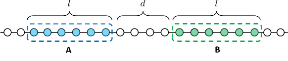
Figure 6: Two spatial symmetric regions A and B in the harmonic chain. $l$ is the comoving size of each region and $d$ is the comoving distance between the two regions. In this case, we consider the coarse-graining scale $n_{\rm{c}}=1$ to investigate the continuous limit of our model.

In Ref. Nambu2008 , the logarithmic negativity of the coarse-grained field in de Sitter space vanishes when the two regions are causally disconnected and FIG. 2 also shows the negativity with the coarse-grained field becomes zero for sufficiently large scales or late times. On the other hand, the negativity obtained without coarse-graining (FIG. 7) does not vanish even when the distance between two regions is larger than the horizon scale ($d_{p}=1$ corresponds to the Hubble horizon scale). This observation confirms that the multipartite entanglement remains on the super horizon scale as expected above. For a vacuum state in the quantum field theory, the Reeh-Schrieder theorem characterizes the (multipartite) entanglement of quantum field Reeh1961 . Our numerical results suggest that the Reeh-Schrieder theorem also holds for the Bunch-Davies vacuum in de Sitter space.

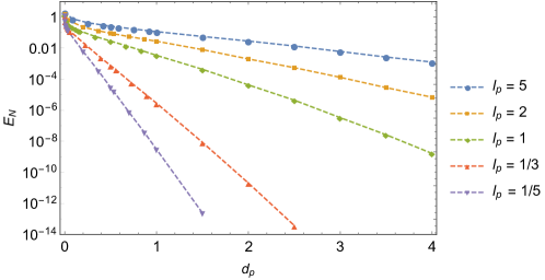
Figure 7: The behavior of the logarithmic negativity $E_{\mathcal{N}}$ as a function of $d_{p}$ with fixed $l_{p}$.

As the Bunch-Davies vacuum approaches to the Minkowski vacuum in the remote past, the behavior of the logarithmic negativity for $l_{p}<1$ and $d_{p}<1$ is expected to be same as that for the Minkowski case. To focus on the entanglement peculiar to de Sitter space, we consider the behavior of the logarithmic negativity for $l_{p}\geq 1$ and $d_{p}\geq 1$. FIG. 8 shows the logarithmic negativity $E_{\mathcal{N}}$ as a function of $d_{p}$ in this case.

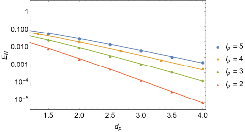
Figure 8: The behavior of the logarithmic negativity $E_{\mathcal{N}}$ as a function of $d_{p}\geq 1$ with fixed $l_{p}\geq 1$.

The logarithmic negativity for $l_{p}\geq 1$ and $d_{p}\geq 1$ behaves as almost linear functions in log plot. We use the fitting function of the exponential factor with the power-law correction to compare with the logarithmic negativity in the Minkowski vacuum Marcovitch2009a . The solid lines in FIG. 8 represent the fitting result

$$E_{\mathcal{N}}^{\text{(fit)}}\approx d_{p}\,e^{-k\,d_{p}},$$ (28)

where $k$ is a real parameter whose values depend on the ratio $l_{p}$. FIG. 9 shows $k$ as a function of $l_{p}$ and the solid line in the figure represents a function $k=a_{1}+a_{2}\,l_{p}^{-1}$ where $a_{1}$ and $a_{2}$ are $O(1)$ constants given by $a_{1}\sim 1.08$ and $a_{2}\sim 4.35$ .

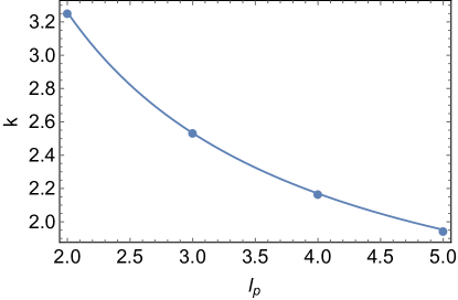
Figure 9: The coefficient $k$ of $d_{p}$ as a function of $l_{p}$.

Combining these, we obtain the following fitting formula of the logarithmic negativity for $d_{p}\geq 1$ and $l_{p}\geq 1$: $E_{\mathcal{N}}^{\text{(fit)}}\approx d_{p}\,e^{-a_{1}d_{p}-a_{2}(d_{p}/l_{p})}$. By restoring the dimension of the variables, this is rewritten as

$$E_{\mathcal{N}}^{\text{(fit)}}\approx\frac{D_{p}}{H^{-1}}\exp\left[-a_{1}\frac{D_{p}}{H^{-1}}-a_{2}\frac{D_{p}}{L_{p}}\right],$$ (29)

where $H^{-1}$ is the Hubble length and the proper size of the region $L_{p}$ and distance $D_{p}$ are given by $L_{p}=a(\eta)\,l\,\Delta x,~{}D_{p}=a(\eta)\,d\,\Delta x$. In the formula (29) we observe that the logarithmic negativity decays exponentially with respect to $H$. This means that the quantum entanglement is degraded by the thermal noise with the Hawking temperature $H$. Thus we consider the value of the numerical factor $a_{1}$ is related to the thermal noise which is independent of details of the theory. On the other hand, the interpretation of the factor $a_{2}$ is not so clear because a value of this coefficient of $D_{p}/L_{p}$ depends on the theory. To make clear its physical interpretation, we will need further analysis of quantum entanglement using other theories of the scalar field in de Sitter space. For the super horizon regions $L_{p}\gg H^{-1}$, the logarithmic negativity (29) becomes independent of the size $L_{p}$ of the two symmetric spatial regions and its value is determined only by the ratio $D_{p}/H^{-1}$. We expect that this property can be understood as follows: the physical wavelength of quantum fluctuation in the considering regions (FIG. 6) is initially smaller than the Hubble horizon. As the universe expands, the wavelength exceeds the Hubble horizon. After the horizon exit, the scale of fluctuations in each region is determined only by the Hubble horizon scale. Hence, the amount of entanglement depends only on $D_{p}/H^{-1}$.

The above property of the logarithmic negativity (29) is expected to be true for the 1+3-dimensional de Sitter space. This is because the feature of the entanglement is determined by the mode function and we use the same mode function as the 1+3-dimensional model. As the quantum fluctuation of super horizon mode is scale independent, the quantum entanglement is determined only by the Hubble scale and the separation between the considering regions.

IV Summary and conclusion

We investigated the quantum entanglement between two symmetric spatial regions with the Bunch-Davies vacuum for the 1+1-dimensional effective harmonic chain model. We introduced the coarse-grained variables and examined the multipartite entanglement in de Sitter spacetime by the monogamy relation of the negativity. In the previous work Nambu2008 , it has been shown that the bipartite entanglement disappears on the super horizon scale. In contrast, in this paper, it was found that the multipartite entanglement of the super horizon scale remains. This indicates that the multipartite entanglement plays an important role to characterize the quantum nature of the the super horizon scale fluctuations. We also considered the continuum limit of our model and calculated the logarithmic negativity for the original canonical variables (without coarse-graining). We confirmed that the logarithmic negativity remains non-zero even if the distance between the two regions becomes larger than the Hubble length. That is, there exists the quantum entanglement between two causally disconnected regions and the existence of the entanglement means that the Reeh-Schrieder theorem holds in de Sitter space.

Finally, we comment on the relation between our lattice model and 1+3-dimensional theory. We considered the 1+1-dimensional effective lattice model of the free massless scalar field in the de Sitter space. As the behavior of the logarithmic negativity depends on the spatial dimension, the numerical simulation in our model is not equivalent to the universe with three spatial dimensions. At the end of Sec. II, we observed that the two-point correlation in our model is larger than it in a 1+3-dimensional de Sitter space. Hence for the scalar field without coarse-graining (continuous limit), if the entanglement disappears for some size and separation of each region in 1+1-dimensional model, we expect that the entanglement in the corresponding 1+3-dimensional model also vanishes. However, according to our numerical calculation, the entanglement in 1+1-dimensional model in the continuous limit exists in any scale. Thus our lattice model provides the necessary condition to judge the existence of quantum entanglement in the 1+3-dimensional de Sitter space. The main features of the logarithmic negativity found in our analysis is characterized by properties of the mode function of the scalar field in de Sitter space. The equation in our model is the same as that in the 1+3-dimensional de Sitter spacetime, and if we evaluate quantum entanglement between spatial regions in the 1+3-dimensional de Sitter spacetime, we expect that we will obtain the similar feature or property of entanglement obtained this paper.

Appendix A Convergence check and violation of uncertainty relation

To confirm that our numerical calculation corresponds to the continuum limit of the lattice model, we check the convergence of the logarithmic negativity. By introducing a scaling parameter $\lambda$, we write other parameters contained in the model as

$$N=200\times\lambda,\quad\alpha=1-\lambda^{-2}\times 10^{-8},\quad l=\lambda.$$ (30)

We regard $E_{\mathcal{N}}$ as a function of $\lambda$ for fixed $l_{p}$ and $d_{p}$. $\lambda\rightarrow\infty$ corresponds to the continuum limit of the model. FIG. 10 shows the result of convergence check.

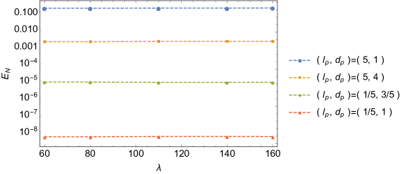
Figure 10: The convergence check of $E_{\mathcal{N}}$ for $(l_{p},d_{p})=(5,1),(5,4),(1/5,3/5),(1/5,1)$. The continuum limit corresponds to $\lambda\rightarrow\infty$.

The logarithmic negativity is independent of the parameter $\lambda$. In the limit $\lambda\gg 1$, length scales (for example, the physical size of the considering region or the distance) is much larger than the UV cutoff $\Delta x$. Hence, this limit corresponds to the continuum limit and our numerical calculation well approaches the continuum limit.

Furthermore, we evaluate violation of the Heisenberg uncertainty relation for our numerical calculation by checking a quantity defined by

$$U_{N}=-\sum_{j=1}^{N}\log_{2}\left[\min{\left(2{\nu}_{j},1\right)}\right],$$ (31)

where ${\nu}_{j}$ are eigenvalues of $i\,\Omega V_{AB}$. If $U_{N}=0$ then we get relations $\nu_{j}\geq 1/2$, which are equivalent to the uncertainty relation. FIG. 11 shows $U_{N}$ as a function of $d_{p}$ for fixed $l_{p}$.

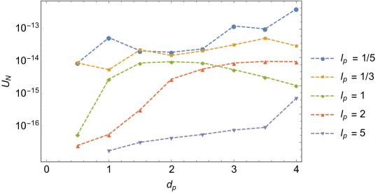
Figure 11: The violation of the Heisenberg uncertainty relation for the fixed ratio $l_{p}=5,2,1,1/3,1/5$ in our numerical calculation. The uncertainty relation holds if $U_{N}=0$ is satisfied.

The uncertainty relation is expressed in terms of the two point functions $\langle\hat{q}\hat{q}\rangle,\langle\hat{p}\hat{p}\rangle$ and $\langle\hat{q}\hat{p}+\hat{p}\hat{q}\rangle$. For the massless theory, the $\hat{q}\hat{q}$-correlation has the IR divergence. On the other hand, there is no the IR divergence in $\hat{p}\hat{p},\hat{q}\hat{p}+\hat{p}\hat{q}$-correlations. In our numerical calculation, owing to behavior of the mode function in de Sitter space, there appears the large difference of the magnitude between the $\hat{q}\hat{q}$- and $\hat{p}\hat{p},\hat{q}\hat{p}+\hat{p}\hat{q}$-correlations. The violation of the uncertainty relation due to numerical error tends to become larger as $d_{p}$ increases. According to FIG. 11, this violation of the Heisenberg uncertainty relation is kept small enough to guarantee accuracy of our numerical calculation.

References

- (1) J. Bell, “On the Einstein Podolsky Rosen paradox”, Physics (College. Park. Md). 1, (1964) 195–200.
- (2) J. Clauser, M. Horne, A. Shimony, and R. Holt, “Proposed Experiment to Test Local Hidden-Variable Theories”, Phys. Rev. Lett. 23, (1969) 880–884.
- (3) M. A. Nielsen and I. L. Chuang, Quantum computation and Quantum Information (Cambridge University Press, 2000).
- (4) S. Marcovitch, A. Retzker, M. Plenio, and B. Reznik, “Critical and noncritical long-range entanglement in Klein-Gordon fields”, Phys. Rev. A 80, (2009) 012325.
- (5) G. Vidal and R. Werner, “Computable measure of entanglement”, Phys. Rev. A 65, (2002) 032314.
- (6) M. B. Plenio, “Logarithmic Negativity : A Full Entanglement Monotone That is nor Convex”, Phys. Rev. Lett 95, (2005) 090503.
- (7) H. Reeh and S. Schlieder, Nuovo Cimento 22,105 (1961).
- (8) J. Maldacena, “Entanglement entropy in de Sitter space”, J. High Energy Phys. 2, (2012) 38.
- (9) Y. Nambu, “Entanglement of quantum fluctuations in the inflationary universe”, Phys. Rev. D 78, (2008) 044023.
- (10) Y. Nambu and Y. Ohsumi, “Classical and quantum correlations of scalar field in the inflationary universe”, Phys. Rev. D 84, (2011) 044028.
- (11) S. Kanno, J. P. Shock, and J. Soda, “Entanglement negativity in the multiverse”, J. Cosmol. Astropart. Phys. 2015, (2015) 015–015.
- (12) S. Kanno, “Impact of quantum entanglement on spectrum of cosmological fluctuations”, J. Cosmol. Astropart. Phys. 2014, (2014) 029–029.
- (13) A. H. Guth and S.-Y. Pi, “Quantum mechanics of the scalar field in the new inflationary universe”, Phys. Rev. D 32, (1985) 1899–1920.
- (14) D. Polarski and A. A. Starobinsky, “Semiclassicality and decoherence of cosmological perturbations”, Class. Quantum Grav. 13, (1996) 377–391.
- (15) J. Lesgourgues, D. Polarski, and A. A. Starobinsky, “Quantum-to-classical Transition of Cosmological Perturbations for Non-vacuum Initial States”, Nucl. Phys. B 497, (1997) 479–508.
- (16) C. Kiefer, J. Lesgourgues, D. Polarski, and A. A. Starobinsky, “The coherence of primordial fluctuations produced during inflation”, Class. Quantum Grav. 15, (1998) L67–L72.
- (17) C. Kiefer, I. Lohmar, D. Polarski, and A. A. Starobinsky, “Pointer States for Primordial Fluctuations in Inflationary Cosmology”, Class. Quantum Grav. 24, (2007) 1699–1718.
- (18) C. P. Burgess, R. Holman, and D. Hoover, “Decoherence of inflationary primordial fluctuations”, Phys. Rev. D 77, (2008) 063534.
- (19) J. Anders and A. Winter, “Entanglement and separability of quantum harmonic oscillator systems at finite temperature”, Quant. Inf. and Comp., 8 (3 & 4), 0245–0262 (2008)
- (20) C. Jaekel, “The Reeh-Schlieder property for thermal field theories”, J.Math.Phys., 41, 1745–1754 (2000)
- (21) H. Narnhofer, “Separability for lattice systems at high temperature”, Phys. Rev. A, 71, 052326 (2005)
- (22) R. Simon, “Peres-Horodecki Separability Criterion for Continuous Variable Systems”, Phys. Rev. Lett. 84, (2000) 2726–2729.
- (23) G. Giedke, L. M. Duan, J. I. Cirac, and P. Zoller, “Distillability Criterion for all Bipartite Gaussian States”, Quantum Inf. Comput. 1, (2001) 79–86.
- (24) T. J. Osborne and F. Verstraete, “General Monogamy Inequality for Bipartite Qubit Entanglement”, Phys. Rev. Lett. 96, 220503 (2006).
- (25) T. Hiroshima, G. Adesso, and F. Illuminati, “Monogamy Inequality for Distributed Gaussian Entanglement”, Phys. Rev. Lett. 98, 050503 (2007) 79–86.