Statistics of shared components in complex component systems

Abstract

Many complex systems are modular. Such systems can be represented as “component systems”, i.e., sets of elementary components, such as LEGO bricks in LEGO sets. The bricks found in a LEGO set reflect a target architecture, which can be built following a set-specific list of instructions. In other component systems, instead, the underlying functional design and constraints are not obvious a priori, and their detection is often a challenge of both scientific and practical importance, requiring a clear understanding of component statistics. Importantly, some quantitative invariants appear to be common to many component systems, most notably a common broad distribution of component abundances, which often resembles the well-known Zipf’s law. Such “laws” affect in a general and non-trivial way the component statistics, potentially hindering the identification of system-specific functional constraints or generative processes. Here, we specifically focus on the statistics of shared components, i.e., the distribution of the number of components shared by different system-realizations, such as the common bricks found in different LEGO sets. To account for the effects of component heterogeneity, we consider a simple null model, which builds system-realizations by random draws from a universe of possible components. Under general assumptions on abundance heterogeneity, we provide analytical estimates of component occurrence, which quantify exhaustively the statistics of shared components. Surprisingly, this simple null model can positively explain important features of empirical component-occurrence distributions obtained from large-scale data on bacterial genomes, LEGO sets, and book chapters. Specific architectural features and functional constraints can be detected from occurrence patterns as deviations from these null predictions, as we show for the illustrative case of the “core” genome in bacteria.

I Introduction

A large number of complex systems in very different contexts - ranging from biology to linguistics, social sciences and technology - can be broken down to clearly defined basic building blocks or components. For example, books are composed of words, genomes of genes, and many technological systems are assemblies of simple modules. Once components are identified, a specific realization of a system (e.g., a specific book, a LEGO set, a genome) can be represented by its parts list, which is the subset of the possible elementary components (e.g. words, bricks, genes), with their abundances, present in the realization. We use the term “component systems” for empirical systems to which this general representation can be applied.

Occurrence patterns of components across realizations are expected to reveal relevant architectural constraints. For example, the bricks present in each LEGO set clearly reflect a target architecture that can be built with them following the instruction booklet. While for LEGO sets the assembly instructions are provided by the seller, in most component systems the architectural constraints are not obvious. Inferring such constraints from the statistics of components may answer important questions about the nature of a system. For example, it could reveal new clues about the complex combination of selective pressure and random events that shaped the functional composition of extant genomes. Even in those cases where the architecture is partially or even fully known and the instruction manual is available, the statistics of components may help us distill some general principles characterizing a given class of component systems, in some cases revealing basic features of the underlying generative processes.

In order to perform detection of system-dependent features from patterns of shared components, we need to have a clear idea of the general behavior of component systems even in absence of functional constraints on the presence/absence of specific classes of components. This is by itself a challenging task, as such systems show a large degree of non-trivial universal properties Altmann and Gerlach (2016); Koonin (2011); Cosentino Lagomarsino et al. (2009) that could in principle affect the occurrence statistics. Indeed, several notable quantitative laws can be identified in the composition of component systems of very different nature. This is well known, e.g., in linguistics, where the notorious “Zipf’s law” Zipf (1935) describing the word frequency distribution (or its equivalent rank plot) in a linguistic corpus has been the subject of extensive investigations Zanette and Montemurro (2005); Newman (2005); Lü et al. (2010); Eliazar (2011); Font-Clos and Corral (2015). In this context, the existence of quantitative “universal” laws may in principle provide insights on the cognitive mechanisms of text production, and can have practical applications in data mining and data search techniques Altmann and Gerlach (2016). Analogously, for genomes across the whole tree of life, the number of genes in different evolutionary families is power-law distributed, a discovery that represents one of the first examples of “laws” of the genome sequencing era Huynen and van Nimwegen (1998); Koonin (2011). Such heterogeneous usage of the different basic components, often resulting in an approximately power-law distribution of their frequencies, can be seen as a hallmark of the complexity of component systems Newman (2005).

A large body of theoretical work addresses the origins of this heterogeneity. Several models have emerged in different areas of science, with context-specific ingredients. For example, stochastic processes based on gene duplication, deletion and innovation have been proposed as simple evolutionary models of genome evolution at the basis of the observed heterogeneous component usage Qian et al. (2001); Karev et al. (2002, 2003); Cosentino Lagomarsino et al. (2009). On the other hand, specific communication optimization principles  Mandelbrot (1953); i Cancho and Solé (2003) and stochastic models for text generation Simon (1955); Zanette and Montemurro (2005); Gerlach and Altmann (2013) have been invoked to explain the emergence of Zipf’s law in natural language. In many, but not all, of these models a preferential attachment principle is at the origin of the emergence of the power-law distribution of component frequencies. More importantly, the ubiquity of this emergent behavior raises the question of whether (and to what extent) empirical laws like Zipf’s law are pervasive statistical patterns that transcend system-specific mechanisms Koonin (2011); Baek et al. (2011). In this spirit, the analysis of radically different systems can help the discovery of patterns that descend from pure statistical effects or general principles Baek et al. (2011); Pang and Maslov (2013).

Here, we analyze empirical data from three very different component systems from linguistics (book chapters), genomics (protein domain families in sequenced genomes) and technology (LEGO toys) and we look for general statistical consequences of their heterogeneous frequency distributions. The different data sources considered here reasonably do not share any generative mechanisms, nor are they expected to share the same type of constraints, selection criteria or optimization principles. However, the frequency of their components is heterogeneous and they all obey laws that are similar to Zipf’s.

The marginal statistics that we concentrate on is the fraction of components that are shared among a certain number of realizations. For example, the fraction of LEGO bricks with the same shape found in a given fraction of unequal LEGO boxes. In genomics, this is the so-called “gene-frequency distribution”, which was shown to follow a U-shape at several taxonomic levels Touchon et al. (2009); Koonin and Wolf (2008); Haegeman and Weitz (2012). A U-shape of this distribution of shared components indicates that there is a set of “core” components that are common to most realizations, as well as an enriched set of realization-specific components. This histogram also decays approximately as a power law for rare components, both in genomic data and in technological systems Pang and Maslov (2013). In evolutionary genomics, the origins of this pattern are the focus of a lively debate. The pattern has been rationalized theoretically by neutral or selective population dynamics models Haegeman and Weitz (2012); Lobkovsky et al. (2013); Baumdicker et al. (2012); Collins and Higgs (2012), or as a consequence of functional dependencies among different components Pang and Maslov (2013). For component systems outside of genomics, the distribution of shared components remains under-explored, and is typically neglected by the current debate, for example in linguistics Altmann and Gerlach (2016).

Using theoretical calculations based on random sampling of components (with replacement) from their overall frequencies (estimated by their total abundance across empirical realizations), we show that a distribution of shared components with a power-law behavior is a general feature of component systems not only with Zipf-like component frequency distributions, but also for general power-laws and exponential decay of the overall component frequencies. In other words, a U-shaped distribution of shared components can naturally emerge in component systems with a heterogeneous component usage (which is often the case empirically). Importantly, we quantitatively identify the general features of the system leading to a U-shaped distribution of shared components, a given core size, and a specific decay of the realization-specific bulk of this distribution.

II Data

II.1 Data sources

Genomes.

We used the superfamily classification of protein domains from the SUPERFAMILY database Wilson et al. (2007) considering a set of $R=1061$ prokaryotic genomes (“realizations”) and a total number of different families $N=1531$ (“components”). Protein domain families are the basic modular topologies of folded proteins Orengo and Thornton (2005). Different domains of the same family can be found in each genome in the same or different proteins. As a functional annotation of protein domains in SUPERFAMILY, we considered the SCOP annotations mapped into 7 general function categories, as developed by C. Vogel Vogel and Chothia (2006).

LEGO sets.

The composition in bricks of several LEGO sets ($R=2820$) can be freely downloaded from “http://rebrickable.com”. We excluded from the analysis LEGO sets belonging to the category of “LEGO Technic” since, by construction, they share a very small number of bricks with the classic LEGO toys. Similarly, we did not consider LEGO sets with less than 80 components or belonging to the categories “Educational and Dacta” and “Supplemental” in order to exclude sets that are actually collections of spare parts or additional bricks for other sets.

Texts.

The analyzed linguistic corpus is composed by $R=1721$ book chapters (realizations) of several English books randomly chosen from the most popular ones in the database “http://www.gutenberg.org”. We defined chapters as realizations, instead of entire books, to obtain a corpus with a range of sizes (total number of components per realization) comparable to the one of genomes and LEGO toys (Figure S1). The complete list of books considered is reported in Table S1 of the Supplemental Material (SM). The elementary components are defined as the words regardless of capitalization (e.g. “We” and “we” are considered as the same component).

II.2 Data structure: Matrix representation of component systems

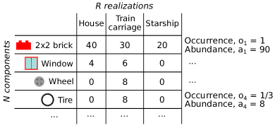
Figure 1: Matrix representation of complex component systems. (a) Each column is a realization (e.g., a LEGO set, a genome or a book chapter) and each row is a component type (e.g., a LEGO brick, a protein domain family, a word). The element $n_{ij}$ represents the abundance of component $i$ in realization $j$. The frequency $f_{i}$ of component $i$ is given by its total abundance ($90$ for the red brick, $8$ for the tire) divided by the total number of components in the system. The occurrence $o_{i}$ of component $i$ is the fraction of realizations (toys in the example) in which there is at least one token of $i$ ($1$ for the red brick, $\frac{1}{3}$ for the tire).

A set of empirical realizations of a component system can be naturally described as a matrix $\{n_{ij}\}$ defined such that the entry $n_{ij}$ represents the abundance of the component $i$ ($i=1,\ldots N$) in the realization $j$ ($j=1,\ldots,R$). Thus, each realization (a literary text, a LEGO set or a prokaryotic genome), is represented as a matrix column (Figure S1). Some key observables can be easily defined using this representation. First, the total abundance $a_{i}$ of the component $i$ in the whole ensemble is defined by summing over all realizations $a_{i}=\sum_{j}n_{ij}$. The normalized abundance represents the component frequency $f_{i}=\frac{a_{i}}{\sum_{i}a_{i}}$.
The “component occurrence” $o_{i}$ is instead defined as the fraction of realizations in which the component is found, thus $o_{i}=\frac{1}{R}\sum_{j}(1-\delta_{n_{ij},0})$.
Two other crucial quantities are: the total number $N$ of different components in the system, which is essentially the number of bricks of different shape or the vocabulary, and the size of a realization $j$, defined as the total number of its components $M_{j}=\sum_{i}n_{ij}$.

III Results

III.1 Component frequency distribution and distribution of shared components show general features across systems

This section illustrates two empirical laws in the analyzed datasets (LEGO toys, bacterial genomes, and literary texts). We first consider the component frequencies in the whole universe of available realizations of a given system, which is essentially the generalized Zipf’s law Newman (2005) for the three systems. Figure S2 shows the rank plots of these component frequencies. The three data sets share a power-law behavior for components with high frequencies (low rank), with an exponent close to 1 as in the classic Zipf’s law Zipf (1935), and a faster decay at higher ranks (components with low frequency). This double-scaling behavior has been recently observed in the context of linguistics Gerlach and Altmann (2013). In evolutionary genomics, the gene frequency was previously analysed over single genomes and shown to be approximately power-law distributed with an exponent dependent on genome size Huynen and van Nimwegen (1998); Cosentino Lagomarsino et al. (2009). Figure S2 shows that the same distribution calculated over thousands of prokaryotic genomes has a double-scaling, with an exponential-like decay for low ranks in its rank plot. We tested that the shape of these component frequency distributions do not strongly depend on the specific size or number of realizations analyzed. The rank plots in Figure S2 do not vary when evaluated on different sub-samples of the whole data sets (Fig. S2 of the SM). This suggests that the frequency distributions evaluated using the available finite empirical data sets estimate reliably the global heterogeneity of the component usage in the systems.

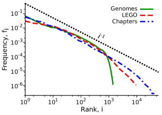
Figure 2: Different empirical component systems show similar component frequency distributions. The rank plot of the component frequencies is reported for the three datasets (book chapters, genomes, LEGO sets). The frequency of a component is defined as the abundance of that component in the whole dataset normalized by the total number of components (Figure S1). The three curves follow similar behavior, which can be described qualitatively as a power-law-like decay with exponent close to $1$ for low ranks (high frequency), and a faster dataset-specific decay for higher ranks.

We aim to evaluate also the distribution of shared components, $\{o_{i}\}$, and how much of its features can be explained from other measurable quantities, namely, the component frequencies, the realization sizes $\{M_{j}\}$ and the number of different components in the universe $N$. Figure S4 shows this distribution for the three data sets considered here. For small occurrences, the plots are compatible with a power-law decay, with a dataset-specific exponent. Only for genomes this curve is clearly U-shaped (see also Fig. S3), and shows a “core” of shared components, i.e., protein domains shared by almost all the genomes, together with a rich group of rare components. Book chapters do not show this marked behavior, due to the fact that the ubiquitous words (e.g. articles, pronouns, prepositions) are much less than the chapter-specific words. Finally, LEGO sets display no core of shared components, and this is probably due to the wide range of themes using poorly overlapping brick types.

Figure 3: The random-sampling model captures the main features of the empirical statistics of shared components. The plots show the normalized distribution $p(o)$ of component occurrences, quantifying the statistics of shared components for the three datasets: genomes (a) book chapters (b) and LEGO sets (c). The log-log scale highlights the power-law like decay. The black dashed lines represent the prediction of the random-sampling model assuming the empirical component frequencies and realization sizes. The model reproduces very well the power-law decay, but may differ quantitatively from the empirical laws in the high-occurrence region. Panel (d) plots the same quantities in log-lin scale, to highlight the quantitative differences between systems and the presence/absence of a peak of core components. Note that the different range of the y-axis values with respect to previous panels is due to the different binning procedures, logarithmic vs linear. (e) Scheme of the random-sampling process: samples of size $M$ are generated from independent draws from the “universe” of all possible components with their specific abundances. Therefore, the probability of a component extraction is proportional to its global abundance, i.e., the sum of its abundances over all realizations of the systems.

III.2 A random-sampling model as a minimal model for component systems with defined component frequencies

In order to identify the statistical consequences of a heterogeneous usage of components on the statistics of shared components, a suitable model is needed. In particular, we would like to generate system realizations starting from a fixed component frequency distribution without any additional functional information or constraint. To this end, we employ a random-sampling procedure Eliazar (2011); van Leijenhorst and Van der Weide (2005); Petersen et al. (2012); Gerlach and Altmann (2013) that builds artificial realizations through an iterative random extraction (with replacement) of components from their frequencies $\{f_{i}\}$ in the whole system. Each realization size $M$ is specified by the number of random extractions.

More precisely, the following prescriptions (Fig. S4e) define the random-sampling model that will be used in the following. (i) The component abundance rank distribution is assumed to be a universal property of the component system and well represented by the empirical overall abundances (see Fig. S2 and the SM for a discussion of this assumption). (ii) The extraction probability of a component is proportional to its overall abundance. (iii) A realization of size $M$ is generated by $M$ independent extractions from the pool of components. Statements (ii) and (iii) define a multinomial process. Given a normalized list of component frequencies $\{f_{i}\}$, $i=1,\ldots N$ (where N is the size of the available “vocabulary”), and the size $M$ of the realization, the probability of a specific configuration $\{n_{1},n_{2},\ldots,n_{N}\}$, where $n_{i}$ is the number of the components with frequency $f_{i}$ is

$$P(n_{1},n_{2},\ldots,n_{N};M)=\frac{M!}{\prod_{i=1}^{N}n_{i}!}\prod_{i=1}^{N}f_{i}^{n_{i}}$$ (1)

under the constraint that $\sum_{i=1}^{N}n_{i}=M$. Note that the expected value of $n_{i}$ is $Mf_{i}$. Therefore, on average the global abundance distribution is conserved in each realization. In other words, the component composition in each realization is a sampled copy of the universe, without any of the possible complex correlations which may follow from architectural and functional properties of an empirical system.

For example, in the context of bacterial genome evolution, the random-sampling model translates into a scenario in which there is continuous and completely random horizontal gene transfer (exchange of genetic material) between species Lobkovsky et al. (2014). Thus, genome composition would simply reflect the pan-genome abundances of protein domains. While horizontal gene transfer is indeed a major force in bacterial evolution Koonin and Wolf (2008); Soucy et al. (2015); Dixit et al. (2015), several additional genome-specific functional constraints are clearly in place in evolution van Nimwegen (2003); Molina and van Nimwegen (2009); Maslov et al. (2009); Grilli et al. (2011); Soucy et al. (2015) and these are neglected by the model. Therefore, the random sampling can be considered as a null model useful to disentangle the consequences of the observed global heterogeneity in the component usage from actual hallmarks of more complex functional constraints.

III.3 The distribution of shared components is mainly a consequence of component frequencies, number of available components and realization sizes

The fact that the distribution of shared components is qualitatively very similar in systems that are so different triggers the question of whether it may be an emergent statistical consequence of other system properties. In particular, we asked to what extent the statistics of shared components could be a direct consequence of component frequencies. As explained above, this question can be addressed quantitatively using a random-sampling model that generates an artificial copy of the empirical system by drawing realizations (whose sizes are fixed by the empirical ones) from the component frequency distribution. Figure S4 compares the empirical occurrence distributions with simulations of a random sampling. The null-model curves (dashed lines) provide very good approximations of the empirical laws, particularly for low component occurrences. Additionally, the model matches well the power law decay with the system-specific exponent. Finally, the model predicts also the qualitative behavior of core components, and specifically that only genomes show a clear U-shaped distribution of shared components. The relative core sizes of the three systems are also well approximated, although there are some quantitative deviations from the empirical values that will be addressed in detail in Section III.6. These results suggest that the shape of the distribution of shared components in the three widely different empirical systems considered here is well described by a random-sampling model that only conserves the empirical component frequencies, the vocabulary (i.e., the set of possible components) and the realization sizes. The next section provides an analytical understanding of this observation.

III.4 A wide range of component frequency patterns lead to occurrence distributions with power-law decay and U-shape.

Thus far, we have used the model only to address the specific statistics of component sharing of the empirical systems under consideration. To this end, we have simulated the random-sampling model fixing the component frequencies and realization sizes as in the empirical cases. More in general, one can ask whether a power-law decaying and/or U-shaped distribution of component occurrences are expected for a given distribution of component frequencies. To address this question, we have computed analytically the distribution of shared components under general prescriptions for the component frequency distributions within the random-sampling model.

For the sampling procedure explained in Section III.2, the probability $q_{i}$ that a component of rank $i$ is present in a realization of size $M_{j}$ is $q_{i}(M_{j})=1-(1-f_{i})^{M_{j}}$, where $f_{i}$ is the component probability of extraction. Therefore, the expectation value for the occurrence of component $i$ over a set of $R$ realizations is

$$o_{i}=\frac{1}{R}\sum_{j=1}^{R}q_{i}(M_{j})=1-\frac{1}{R}\sum_{j=1}^{R}(1-f_{i})^{M_{j}}\ .$$ (2)

In order to obtain the probability distribution associated to this rank representation, one can use the fact that the rank of a component with occurrence $o$ is the number of components with occurrence higher than $o$. In fact, these naturally correspond to components with higher frequency and thus lower rank. Therefore, we can write the rank $i(o)$ as

$$i(o)=\text{rank}(o)=\sum_{o^{\prime}=o}^{o_{1}}Np(o^{\prime})\simeq N\int_{o}^{o_{1}}p(o^{\prime})do^{\prime}\ ,$$ (3)

where $o_{1}$ is the highest possible occurrence, which corresponds to the component of rank 1. The function $i(o)$ is simply the inverse function of Eq. 2. From the approximate integral representation of $i(o)$, the occurrence probability distribution $p(o)$ is defined by the simple relation $\frac{di(o)}{do}=-Np(o)$.

Eq. 3 provides a general relation between the representation of the frequency distribution as a rank plot and the representation as a probability distribution. Indeed, the arguments presented here to introduce Eqs. 2 and 3 have been previously used to establish the connection between Zipf’s law as a rank plot and Zipf’s law as a frequency distribution Mitzenmacher (2004).

III.4.1 Observed versus possible vocabulary of components and Heaps’ law

When a set of $R$ realizations of size $M$ is generated through a random-sampling procedure from a pool of $\tilde{N}$ possible different components with their probabilities of extraction $\{f_{i}\}$, the expected size $N$ of the vocabulary that is actually sampled can be expressed as van Leijenhorst and Van der Weide (2005)

$$N=\tilde{N}-\sum_{i=1}^{\tilde{N}}\left(1-f_{i}\right)^{MR}\ .$$ (4)

Thus, in general, $N\leq\tilde{N}$.

If the system size, defined by the total number of extractions $MR$, is large enough, essentially all possible components are expected to be sampled at least once, thus leading to the simplification $N\simeq\tilde{N}$ that we implicitely assumed in Eq. 1. However, in general, the observed vocabulary in an ensemble of realizations is an increasing function of the system size, i.e., $N(MR)$. This functional dependence is the analogous of Heaps’ law, which is the empirical power-law growth of the number distinct components with the system size observed in linguistics Altmann and Gerlach (2016); Gerlach and Altmann (2013), and in genomics Cosentino Lagomarsino et al. (2009). This distinction between the observed and the possible vocabulary of components is discussed in more detail in the SM and will be relevant in the following sections.

III.4.2 Analytical distribution of shared components for component frequencies with a power-law or an exponential distribution

Explicit expressions for the occurrence distribution can be derived assuming a simple scenario, in which all realizations have the same size $M$, and the component frequency statistics follows a prescribed function. We first consider the empirically relevant case of a power-law frequency rank plot (Fig. 4, left panel) defined by

$$f_{i}=\frac{1}{\alpha}i^{-\gamma},\hskip 28.45274pt\alpha=\sum_{i=1}^{\tilde{N}}i^{-\gamma}\ .$$ (5)

Under these assumptions and using Eqs. 2 and 3, the exact expression of the occurrence distribution can be calculated:

$$p(o)=\frac{\left(1-o\right)^{\frac{1}{M}-1}}{\gamma MN\alpha^{\frac{1}{\gamma}}\left(1-(1-o)^{\frac{1}{M}}\right)^{\frac{1}{\gamma}+1}}\ .$$ (6)

The distribution is defined in the interval of occurrences $[o_{N};o_{1}]$, where $o_{i}$ is computed by Eq. 2 and $N$ is the effective or observed component vocabulary, which can be a function of the system size, i.e., $N(MR)$, as described by Eq. 4. Considering the limit of small occurrences and large sizes, i.e., $o\ll 1$ and $M\gg 1$, one finds precisely the empirically observed power-law decay. Specifically, in this limit the occurrence distribution takes the form

$$p(o)\simeq\frac{M^{\frac{1}{\gamma}}}{\alpha^{\frac{1}{\gamma}}\gamma N}o^{-\frac{1}{\gamma}-1}\ ,$$ (7)

where the power-law exponent depends only on the exponent $\gamma$ of the frequency rank-plot .

Analogous calculations (details in the SM) can be performed assuming a frequency distribution described by an exponential rank plot $f_{i}\sim e^{-\lambda i}$ (right panel of Figure 4). In this case, the distribution of shared components, for large enough realizations $M\gg 1$, has the expression

$$p(o)\simeq\frac{(1-o)^{-1}}{N\lambda\log{\left[(1-o)^{-1}\right]}}.$$ (8)

Interestingly, for rare families the above expression further simplifies to a power-law decay

$$p(o)\simeq\frac{1}{N\lambda}o^{-1},$$ (9)

with a “universal” exponent $-1$. This indicates that also systems with a heterogeneous but more compact frequency distribution are expected to show a power-law decay in the occurrence distribution. Figure 4 shows the agreement between these predictions and simulations of the random-sampling model for the two illustrative examples of a power law and of an exponential distribution of component frequencies. These analytical predictions have a dependence on the sampled vocabulary $N$ and are expected to hold even if this is actually smaller than the total number of possible components $\tilde{N}$ (Fig. S5). The effects of a dependence of the observed dictionary on system size (i.e., Heaps’ law $N(MR)$) become relevant and has to be taken into account when comparing statistical features of ensembles of realizations with different sizes $MR$.

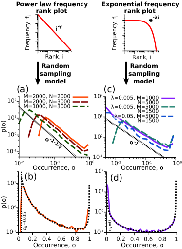
Figure 4: Power-law decaying and U-shaped component occurrence distributions may descend from both power-law and exponential distributed universe component frequencies. (a): A power-law rank-plot for the frequency (and thus for the abundance), whose exponent is $-\gamma$ ($\gamma=1.2$ in the plot), produces a power-law decay of the component occurrence distribution with exponent $-1-\frac{1}{\gamma}$, independently of the realization size $M$ and the number of components $N$ (for sufficiently large values of these parameters). (b): Agreement between the theoretical prediction of Eq 6 (black line) and a simulated random sampling with parameters $R=1000$, $N=2000$, $\gamma=1.2$, $M=2000$ (the black vertical dashed line is the left boundary of the $p(o)$ domain). Panels (c) and (d) are the counterpart of (a) and (b) for an exponential frequency rank plot. In this case $p(o)$ always decreases with exponent $-1$, for every value of $\lambda$, $M$, and $N$ (sufficiently large). Parameter values: $R=1000$, $N=2000$, $\lambda=0.005$, $M=5000$. Given the system sizes $MR$ in these examples, the number of possible different components essentially coincides with the vocabulary actually sampled , i.e., $\tilde{N}\simeq N$.

III.4.3 Shape of the distribution of shared components and rescaling properties

We now turn our attention to the conditions for a U-shaped distribution of shared components in the random-sampling model. Figure 4ac already show that the decay of the occurrence of rare components is only set by the exponent $\gamma$ as described by Eq. 7, but for different values of $M$ and $N$ the distribution may or may not display a significant fraction of core components. Additionally, Figure 4bd proves that equations (6) and (8) can capture quantitatively the occurrence distributions and thus can well describe the relative proportion of core and specific components. In order to understand under what conditions this distribution becomes clearly U-shaped for an underlying power-law frequency distribution, it is useful to note a rescaling property of Eq. 6. Taking the limit of large realizations $M\gg 1$, Eq. 6 becomes

$$p(o)=k(\gamma,M,N)\frac{(1-o)^{-1}}{\gamma\left(-\log(1-o)\right)^{1+\frac{1}{\gamma}}},$$ (10)

which depends only on two parameters, $\gamma$ and the rescaling parameter

$$k(\gamma,M,N)=\frac{M^{\frac{1}{\gamma}}}{\alpha^{\frac{1}{\gamma}}N}\ .$$ (11)

This rescaling property shows that the statistics of component sharing is actually a function of a specific combination of realization sizes (e.g., text lengths) and of the range of possible components (e.g., the observed vocabulary). Specifically, the functional form of the distribution is purely defined by the exponent $\gamma$, while the rescaling parameter $k$ sets the normalization factor and the range of possible occurrences. In fact, the analytical expression of the occurence corresponding to the distribution minimum, i.e., $o_{min}=1-e^{-1-\frac{1}{\gamma}}$, is only a function of $\gamma$, while the minimum possible occurrence value $o_{N}\simeq 1-e^{-k^{\gamma}}$ scales with $k$. Therefore, a U-shaped occurrence distribution should be generally expected for component systems with highly heterogeneous component frequencies since the power-law decay and the presence of a minimum before the core are robust features with respect to system parameters. This is confirmed by the analysis of component systems with different values of $k$ and $\gamma$ (illustrative examples in Figure S7): the system specificities set the power-law decay of the left part of the distribution, its support, and the relative proportion of core and rare components, but the U-shape is conserved. However, this shape can be more or less symmetric and more or less clearly evident depending on the actual size of the core fraction. The following section discusses in detail the non-trivial dependences of the core size on system parameters.

For the case of component frequency distributions with an exponential rank plot, the statistics of shared components (Eq. 8) is a function of a single effective parameter $\lambda N$, and does not depend on the realization sizes $M$. In other words, the shape of the distribution, and whether it is clearly U-shaped, only depend on the decay of component frequencies and on the total number of components. In fact, occurrence distributions corresponding to different exponential frequency rank plots collapse if $\lambda N$ is constant, even if the realizations have widely different size. This is shown in Figure S4 of the SM.

III.4.4 The core size

We can estimate the “core size” by computing the fraction of components with occurrence greater than a given arbitrary occurrence threshold $\theta_{c}$ as a function of the only two effective parameters $\gamma$ and $k$. Integrating Eq. 6 between $\theta_{c}$ and the maximum occurrence $o_{1}$, and then taking the limit $M\gg 1$, this quantity reads

$$\begin{cases}c=1&\text{if}\hskip 8.5359pto_{N}\geq\theta_{c}\\ c=k\left[-\log(1-\theta_{c})\right]^{-\frac{1}{\gamma}}&\text{otherwise}\end{cases}\ ,$$ (12)

where $o_{N}$ is the left boundary of the occurrence distribution, corresponding to the component with lowest frequency.

Starting from this estimate of the core size, Figure 5ab show how the scaling property is verified in simulations. Fig. 5c compares the analytical predictions for the core size with simulations for different values of $\gamma$, showing perfect agreement. Equally, one can obtain analytical estimates for the fraction of rare components (occurrence below a fixed threshold), which are tested in Fig. 5d. Thus, with increasing $k$, core families increase linearly with a $\gamma$-dependent slope until all components are shared, and concurrently rare components decrease linearly until they hit zero (when the lower cutoff of occurrence exceeds the chosen threshold value). Component number and realization size only enter through the combination defined by the rescaling parameter $k$. This phenomenology fully characterizes the distribution of shared components with varying parameters.

The general relation (Eq. 12) between the core size and the rescaling parameter $k$ translates into different dependences of the core size on the typical realization size $M$, depending on the relation between the system size $MR$ and the total number of accessible components $\tilde{N}$. While this issue is discussed in more detail in the SM, it is easy to intuitively understand the different regimes. For large enough systems, all possible components $\tilde{N}$ are expected to be sampled at least once, thus making the observed vocabulary $N\simeq\tilde{N}$ a constant parameter. This is the regime considered in Fig. 5a. In this regime, Eq. 12 simplifies to the simple scaling $c\sim\frac{M^{\frac{1}{\gamma}}}{\tilde{N}}$. On the other hand, in several empirical systems the observed vocabulary is a function of the system size, and typically with the power-law dependence $N(MR)\sim(MR)^{\beta}$ (with $\beta<1$) called Heaps’ law. Thus, in general, the core fraction is expected to show the more complex dependences $c\sim M^{\frac{1}{\gamma}-\beta}R^{-\beta}$. However, a random-sampling procedure starting from a Zipf’s law described by Eq. 5 leads to the approximate relation $\beta\simeq 1/\gamma$ between the exponents of Zipf’s and Heaps’ law Eliazar (2011); van Leijenhorst and Van der Weide (2005); Lü et al. (2010). Therefore, in this regime the core fraction becomes only a function of the number of realizations as $c\sim R^{\frac{1}{\gamma}}$. These different scaling relations in different regimes are tested in Figure S6. Note that the absolute number of core components $cN$, as estimated from Eqs. 11 and 12, is instead always independent from the number of realizations, even in the regime where Heaps’ law is expected to hold (Figure S6).

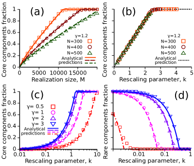
Figure 5: Scaling of the distribution of shared components and fraction of rare and core components. (a) The fraction of core components (defined by the occurrence threshold $o>\theta_{c}=0.95$) for a power-law component frequency distribution with exponent $\gamma=1.2$, plotted as a function of component size $M$ for three values of realization number $N$. (b) Collapse of the curves shown in panel (a) when plotted as a function of the rescaled parameter $k$, defined in Eq. 11. (c) and (d): fraction of core and rare ($o<0.05$) plotted as a function of $k$ for different values of $\gamma$. For sufficiently large $k$ (i.e. typically when $M$ dominates over $N$), the fraction of core components saturates to $1$. Conversely, the fraction rare components drops to zero for increasing $k$. Symbols refer to numerical simulations of the random-sampling model, while the lines are the theoretical predictions of Eq. 12.

For component frequency distributions with an exponential rank plot, the sampling procedure leads to an occurrence distribution that is independent from the realization size $M$ (Eq. 8). However, the exact analytical prediction for the core size (the analogous of Eq. 12) still has a dependence on $M$. But this is due to the residual dependence of the maximum occurrence values ($o_{1}$) on $M$ and does not affect the shape of the distribution. This last technical point is discussed in more detail in the SM.

III.5 Empirical distributions of shared components satisfy the relations predicted by the random sampling.

One can ask whether the general analytical predictions discussed in the previous section can be applied to empirical data. In particular, we first asked how the power-law decay exponent of the distribution of shared components relates to the component frequency rank plot in empirical systems, and if this relation follows our analytical prediction. An analytical mapping would give a more synthetic and powerful description than the direct simulations discussed in Fig. S4. Importantly, the analytical formulas for the distribution of shared components are derived under the hypothesis of a pure power-law or exponential component frequency rank plot. However, the three empirical datasets (as previously discussed), show a double-scaling frequency distribution. To override this issue, we restricted the frequency rank plot range in which the predictions are applicable. The procedure to perform this comparison is described in Fig. 6.

First, we chose an arbitrary threshold $\theta_{r}$ defining the rare components and we mapped it to the frequency rank plot (assuming the model), by using the inverse function of Eq. 2. The frequency rank associated to the occurrence threshold $\theta_{r}$, $i(\theta_{r})$ in the figure, is the rank above which the model prediction for the decay of the distribution of shared components should apply as long as $i(\theta_{r})$ does not cross the position of the change in scaling. In other words, since in the model there is a monotonic relation between occurrence and frequency (Eq. 2), all components with rank greater than $i(\theta_{r})$ (and frequency smaller that $f_{i(\theta_{r})}$) are assumed to be the components with occurrence lower than $\theta_{r}$. We then estimated the behavior of the frequency rank plot in the high-rank region (after $i(\theta_{r})$) as the best fit with a power-law function or an exponential. This leads to a prediction for the decay exponent of the distribution of shared components (using Eq. 7 or Eq. 9 for the exponential case) in the range $[o_{N},\theta_{r}]$. Fig. 6 shows that the predicted decay exponents correspond well with the data.

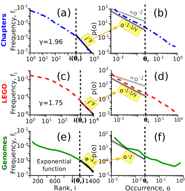
Figure 6: The relation between the exponents of frequency rank plot and occurrence distribution is satisfied in all the three datasets. The plots consider the low occurrence region, below the arbitrary threshold $\theta_{r}=0.025$ which corresponds to the high-rank region above $i(\theta_{r})$ in the frequency rank plot (see main text). Panel (a) and (b) refer to book chapters, for which the tail of rank plot is a power law with exponent $\gamma=1.96$, which implies a power law decay of $p(o)$ with exponent $1+\frac{1}{\gamma}=1.51$. Panel (c) and (d) show the LEGO dataset ($\gamma=2.8$, $1+\frac{1}{\gamma}=1.36$). Panel (e) and (f) correspond to protein domains in genomes, where the best fit of the tail region the rank plot is an exponential function (note that (e) is in linear-logarithmic scale), which implies a power law decay with exponent $-1$.

The random-sampling model also gives qualitative analytical predictions for the expected fraction of core components, and thus for the expected shape of the distribution of shared components for a given empirical system. While the analytical relations between exponents applied in Figure 6 do not depend on the realization sizes, the analytical formulas for the fraction of core components (see e.g. Eq. 12) were derived assuming realizations of fixed size $M$. The actual size distributions for the three empirical systems are quite broad (Figure S1), but we can still use the analytical framework to get an estimate of the core fraction considering the average realization size of each empirical system. Following the same line of reasoning as for the low-occurrence tail of the distribution of shared components, we can use a restricted region of the frequency rank plot. In this case, the low-rank region (with exponent around $1$ for all the datasets, see Fig. S2) is expected to contain the core components. Therefore, the parameter $\gamma$ can be fixed to $1$, implying that the fraction of core components, given by Eq. 12, should be simply proportional to the rescaling parameter $k$ (Eq. 11). However, the normalization factor $\alpha$, which is present in the definition of $k$ and defined in Eq. 5, takes an approximately constant value with respect to $\tilde{N}$ for large values of $\tilde{N}$, as it is the case for the empirical examples considered. As a consequence, the core fraction should be simply proportional to $\frac{M}{N}$. This estimate can be used to explain why the core fraction is much larger in genomes than in the other two empirical systems (see Figure S2d). In fact, genome sizes are typically of the same order as the total number of families ($M\simeq 3000$, $N=1531$, see Figure S1) leading to a large expected core. By comparison, book chapters have similar realization sizes but a much larger vocabulary ($N\simeq 50000$), and LEGO sets have very small sizes ($M\simeq 100$) compared to vocabulary size ($N\simeq 13000$).

More in general, Eqs. (11) and (12) lead to a scaling estimate (dependent on the decay of the frequency rank plot) as a function of the system parameters $M$ and $N$, which can be applied to data, in order to generate expectations for the core components. For example, for Zipf-like (exponent -1) frequency distributions, we expect the absolute number of core components to be linearly dependent on the average size of realizations $M$, and essentially insensitive to the vocabulary size $N$ and the total number of realizations $R$. In genomics language, this would imply that the number of core protein domains does not directly depend on the number of sequenced genomes but only on their sizes and on the total number of different protein domains discovered. Note that adding new genomes to the data set is not expected to alter the power-law exponent $\gamma~{}\simeq 1$ of the global frequency distribution for high-frequency components, since it does not change if the distribution is evaluated on sub-samples of the empirical dataset (Figure S2).
As previously discussed, the core fraction, instead of the absolute number of core components, is expected to have a more complex dependence on the typical realization size $M$ and on the number of realizations $R$. Moreover, in empirical systems these relations are further complicated by the fact that the frequency distributions cannot be described by simple power-laws (Fig. S2). Nevertheless, the relation between the core fraction and the average realization size predicted by a random-sampling model can be tested numerically, as Figure 7a shows for prokaryotic genomes, and seems accurately verified and roughly linear in the tested range of sizes. However, the predicted fraction of core components is actually much smaller than the empirical one. This highlights the presence of additional functional constraints and/or specific correlations in the empirical system that the model can not capture. The next section addresses this point more in detail.

III.6 Deviations from the random-sampling predictions can highlight system-specific properties

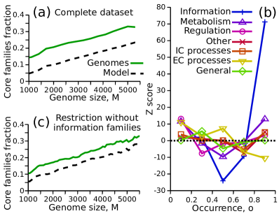
Figure 7: Specific functional constraints can be detected by deviations from the predictions of a random sampling. a) Fraction of common protein domain families as a function of the genome sizes. Each point of the curves corresponds to the core families ($o>\theta_{c}=0.95$) given the occurrence distribution of a genomes’ subset whose sizes are inside a certain window. The average of the size windows defines the x axis. b) Enrichment analysis in the occurrence distribution for specific functional categories. Considering domain families relative to a single functional category, their relative component occurrence distribution was evaluated for an ensemble of systems built with a random sampling. From this, the average value and the standard deviation for the expected fraction of components at each occurrence value $o$ can be calculated. This provides a measure (Z score) of over- or under-representation of domain families belonging to each functional category in the empirical dataset. c) Excluding from the analysis the domain families associated to information processes (i.e., DNA replication, transcription and translation) significantly reduces the offset between the random-sampling prediction and the empirical trend.

Beyond the striking agreement with null predictions for shared components, the deviations from sampling can be used to quantify specific functional and architectural features of a component system. While the scope of this work is to highlight the common trends and their origins, we discuss a specific example, in order to show the feasibility of this procedure. Of the three data sets considered here, the case where the clearest deviations emerge are genomes. For example, Figure 7a illustrates how the random sampling underestimates the empirical core size by a constant offset, for genomes of increasing size. Generally speaking, this larger core of components is due to the components that tend to occur in most realizations, but in few copies. The natural explanation is that there are specific basic functions that are essential for all (or most) genomes, but the domains involved in these functions are not necessarily needed in many copies per genome, and thus their presence in all realizations does not simply correlate with high global abundances as the random sampling would entail Koonin (2003).

To test this hypothesis, we divided the domain families in functional categories (see Section II for the functional annotation), and tested if most of the deviations from the random-sampling prediction can be ascribed to the statistics of domains belonging to specific categories. The result of this analysis is reported in Figure 7b. Different parts of the distribution of shared components are indeed enriched in components of different biological functions with respect to the random-sampling expectation. In particular, protein domains that play a functional role in information processes - such as DNA translation, DNA transcription, and DNA replication- are clearly enriched in the core. At the same time, they seem statistically under-represented at occurrences around 0.6. These two deviations can be explained as two sides of the same coin if this category contains domain families that empirically occur in all genomes but in a single copy per genome. Indeed, the global frequency (i.e, across all genomes) of families that are both single-copy and ubiquitous is $f=\frac{R}{RM}=1/M$. Therefore, their occurrence predicted by the random-sampling model is $o=1-(1-\frac{1}{M})^{M}=1-e^{M\text{log}(1-\frac{1}{M})}\simeq 1-e^{-1}\simeq 0.6$ (where the rough approximation holds for large enough $M$), thus naturally leading to an excess of those families in the core and to a depletion around $o\simeq 0.6$.

The observation of a strong presence of protein domains related to basic cellular function in the core genome is not new Koonin (2003); Koonin and Wolf (2008). However, the random-sampling model allows in principle to distinguish families whose presence in the core could be simply explained by their high abundance in the pan-genome and thus it would be expected also in a simple scenario of random gene exchange. Finally, the observed correlation between biological functions and deviations from random sampling predictions seems coherent with a picture, recently proposed Lobkovsky et al. (2013), in which natural selection and functional constraints have played an important role in defining the empirical U-shaped distribution of gene occurrences.

IV Discussion and Conclusions

This work employs a simple statistical model based on random sampling to describe the distribution of shared components in complex component systems. A similar approach was employed in quantitative linguistics to explain how the dictionary used in a text scales with text size as measured in number of words (the so-called “Heaps’ law”) while assuming Zipf’s law for component frequencies Eliazar (2011); Heaps (1978); van Leijenhorst and Van der Weide (2005); Lü et al. (2010); Font-Clos and Corral (2015). We extended the model to show that there is a general link between the heterogeneity in component frequency and the statistics of shared components, regardless of the mechanisms that generate heterogeneity. Consequently, models or generative processes able to explain the heterogeneity in component frequency implicitly carry predictions for the statistics of shared components.

The striking similarities of laws governing both component abundance and occurrence found in empirical systems of very different origins (LEGO sets, genomes, book chapters) support the idea that the concept of “component system” defined in this work can capture in a unified framework a large class of complex systems with some common global properties. Different component systems, besides having specific architectural constraints, may show convergent phenomena in terms of global statistics. Such “universal” phenomena may be regarded as emergent properties due to system heterogeneity, which transcend the specific design, generative process or selection criteria at the origin of a system. Analogous phenomena occur, for example, in ecosystems, where emergent species-abundance distributions appear for forests, birds or insects Hubbell (2001).

Beyond the examples considered here, modular systems in a wide range of disciplines can be represented as component systems. Developing a common theoretical language for such systems can help the exchange of ideas, models and data-analysis techniques between distant communities of researchers Holovatch et al. (2017). For example, the statistics of component sharing considered here plays a central role in genomics Lapierre and Gogarten (2009); Lobkovsky et al. (2013); Koonin (2011) but is relatively unexplored in the context of natural languages Altmann and Gerlach (2016). Conversely the random-sampling approach used here was developed in quantitative linguistics Eliazar (2011), and this work shows that it is applicable to other systems, including the detection of functional constraints in prokaryotic genome evolution.

An important result of this work is a proof of the clear link between the heterogeneity of component abundance in a system and the statistics of shared components. This link is consistent with data from three very different empirical systems and well captured by the random-sampling model. The fact that emergent patterns can be explained by largely null models resembles again the case of biodiversity, where neutral theories ignoring species interactions and competitive exclusion appear to capture many of the emerging trends of species abundance Hubbell (2001); Azaele et al. (2016).

If the trends of component sharing of generic component systems are to be regarded as largely null and due to components heterogeneity, system-specific investigations should be informed of this general trend. Quantitative null models, such as the one provided here, may be crucial for identifying dataset-specific deviations that are related to functional reasons or constraints. In the data considered in this work, the patterns of shared components show differences between empirical data and the null model in some cases. This is particularly true in the genomic context, where the differences can indeed be traced back to functional constraints in genome composition. Therefore, the framework can be useful to pinpoint hallmarks of functional design and distinguish them from statistical effects, particularly for the detection of causality, dependency and correlation structures between components from occurrence patterns.

Once a null model is defined, these features can emerge as significant deviations from the null behavior, for example as violations of the constraints linking different global statistics such as the abundance rank plot, the distribution of shared components and Heaps’ law. We have considered here a specific example for the case of shared protein domain families in genomes (Fig. 7), but this question still needs to be approached systematically. In this specific case, core components are particularly enriched by specific functional classes of components with respect to the random-sampling prediction. In evolutionary terms, the random sampling defines a scenario in which the pan-genome fully determines the overall abundance of the gene families in each genome, while in empirical bacterial genomes genome-specific functional constraints are clearly in place Maslov et al. (2009); Molina and van Nimwegen (2009); Grilli et al. (2014). Deviations from the null scenario can thus highlight the role of selection for specific functions, supporting from a different perspective the idea that the empirical U-shaped gene occurrence distribution is affected by selective rather than neutral processes Lobkovsky et al. (2013); Collins and Higgs (2012); Baumdicker et al. (2012); Haegeman and Weitz (2012).

SUPPLEMENTAL MATERIAL
Statistics of shared components in complex component systems

S1 Books composing our linguistic corpus

Supplementary Table S1: List of the books whose chapters compose the analyzed linguistic corpus. Data downloaded from the Project Gutenberg: http://www.gutenberg.org

Title	Author
Alice’s adventures in wonderland	Lewis Carroll
Anna Karenina	Lev Nikolayevich Tolstoy
A tale of two cities	Charles Dickens
Dracula	Bram Stoker
Emma	Jane Austen
Great expectations	Charles Dickens
Les miserables	Victor Hugo
Moby Dick	Herman Melville
Notre-Dame de Paris	Victor Hugo
Pride and prejudice	Jane Austen
The adventures of Tom Sawyer	Mark Twain
The count of Monte Cristo	Alexandre Dumas
The man in the iron mask	Alexandre Dumas
The picture of Dorian Gray	Oscar Wilde
The three musketeers	Alexandre Dumas
War and peace	Lev Nikolayevich Tolstoy

S2 Size distributions of the realizations in the three data sets

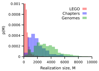
Supplementary Figure S1: Size distributions of prokaryotic genomes, book chapters and LEGO toys. Probability distribution of the realization size $M$, defined as the total number of components (protein domains, words or LEGO bricks) in a realization (genomes, chapters or LEGO sets).

S3 Universality of the component abundance distribution (Zipf’s law)

Figure S2 tests the component frequency rank distribution conservation when it is evaluated on different sub-sets of the total empirical data set. These sub-sets are composed by realizations in a fixed range of sizes, showing that the global frequency statistics does not depend on the realization sizes or on the number of realizations considered. Note that this test is necessary to safely compare the analytical null predictions with different sub-samples of the empirical data set, as for example in Figure 7 of the main text. Moreover, the fact that the Zipf’s laws of the under-sampled datasets is essentially identical to the global one (especially in the high-frequency regime) suggests that the observed Zipf’s law is not under-sampled and can thus be considered a good estimation of the “universal” one.

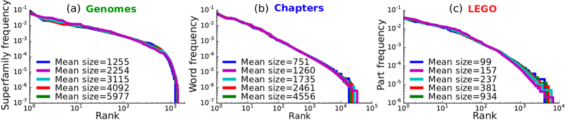
Supplementary Figure S2: Zipf’s law for different sub-samples of the empirical data sets, corresponding to different bins of realization sizes. Zipf’s law in genomes (a), book chapters (b), and LEGO sets (c) for several sub-sets of the data set. The average sizes of the realizations in each sub-set are reported in the legend.

S4 Robustness of the U-shaped distribution of shared components for bacterial genomes to the binning procedure.

Supplementary Figure S3: Robustness of the U-shaped distribution of shared components for bacterial genomes to the binning procedure. The plot is the analogous of Fig. 1d of the main text, but with bins of different sizes. The binning procedure does not influence the shape of the distribution of shared components.

S5 Properties of the occurrence distribution generated by an exponential frequency rank plot

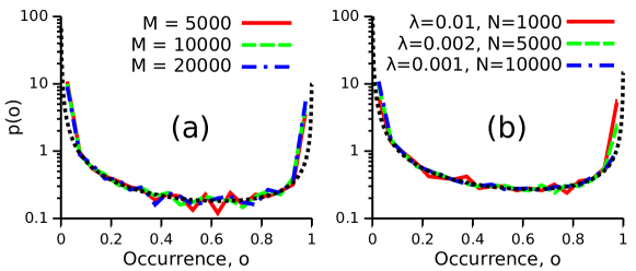
Supplementary Figure S4: Rescaling property of the occurrence distribution generated by an exponential frequency rank distribution. a) The global shape of the distribution does not depend on $M$ in the limit $M\gg 1$, as shown by the Eq. S3. The three curves are computed at fixed values of $\lambda=0.01$ and $N=1500$, and the black dotted line is the prediction of Eq. S3. The only effective parameter determining the U-shape (for $M\gg 1$) is the product $\lambda N$. Indeed, panel b shows that the distribution does not change its shape while varying $N$ and $\lambda$ if their product is kept to a constant.

The mathematical calculation described in the section IIIC of the main text can be applied to an exponential rank distribution of the form

$$f_{i}=\frac{1}{\beta}e^{-\lambda i},\hskip 28.45274pt\beta=\sum_{i=1}^{\tilde{N}}e^{-\lambda i}.$$ (S1)

Considering a random sampling of $R$ realizations with fixed size $M$, one finds:

$$p(o)=\frac{(1-o)^{\frac{1}{M}-1}}{\lambda MN\left(1-(1-o)^{\frac{1}{M}}\right)}.$$ (S2)

Imposing the condition $M\gg 1$ this equation takes the form

$$p(o)\simeq\frac{(1-o)^{-1}}{N\lambda\log{\left[(1-o)^{-1}\right]}},$$ (S3)

which provides a good approximation for the overall distribution shape as a function of one single effective parameter $k=N\lambda$.

In the $M\gg 1$ limit, the occurrence extreme values are $o_{1}\simeq 1$ and $o_{N}\simeq 0$. This implies that the distribution is well defined over all possible values of occurrence. Figure S4 shows the rescaling properties of Eq. S3 by testing its independence on $M$ (panel a) and by varying $N$ and $\lambda$ while keeping their product constant (panel b).

For rare families, one can further approximate the expression for $p(o)$ finding the expected power-law decay with exponent $-1$:

$$p(o)\simeq\frac{1}{N\lambda}o^{-1}.$$ (S4)

We now analyze the properties of the fraction of core components, i.e., those with occurrence greater than the threshold $\theta_{c}$. In order to derive the core size one has to integrate the distribution described by Eq. S2 from $o=\theta_{c}$ to the maximum occurrence value $o_{1}$ (whose formula can be obtained from Eq. 2 of the main text).

The result reads:

$$\begin{cases}c=1&\text{if}\hskip 8.5359pto_{N}\geq\theta_{c}\\ c=-\frac{1}{N\lambda}\left(\lambda+\log{\beta}+\log{\left[1-(1-\theta_{c})^{\frac{1}{M}}\right]}\right)&\text{otherwise}.\end{cases}$$ (S5)

In the limit of large $M$ this expression becomes

$$c\simeq-\frac{1}{N\lambda}\left(\lambda+\log{\beta}+\log{\left[\log{(1-\theta_{c})^{-1}}\right]}-\log{M}\right),$$ (S6)

which further simplifies only when the logarithm of $M$ becomes dominant over the other terms.

It is worth mentioning that the expression above does not show rescaling properties, even in the regime $M\gg 1$, and this may seem to be in contradiction with Eq. S3. Nevertheless, this apparent inconsistency is basically due to the singular behavior of the occurrence distribution in $o\simeq 1$. In the large $M$ limit, the right boundary can be expressed as $o_{1}=1-\epsilon$, where $\epsilon$ is an infinitesimal term depending on $M$ and $\lambda$, whose effect on the overall distribution shape is negligible (Eq. S3). However, the core size is defined as the integral of the distribution. Therefore, the variation of $p(o_{1})$ due to a change in $M$ or $\lambda$ provides a sufficiently large contribution (because of the function singular behavior) which compensates the infinitesimal variation of $o_{1}$. Finally, this leads to a finite contribution to the integral and thus to the core size as it is defined in the main text. In general, this finite contribution has a non-trivial dependency on the parameters, explaining why Eq. S6 does not show the rescaling property.

S6 Difference between observed and possible vocabulary of components (Heaps’ law) and its effects on the core-size estimates.

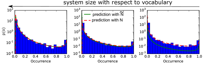
Supplementary Figure S5: Analytical prediction for the occurrence distribution of component systems with different sizes. For large system sizes $MR$ (left panel), essentially all the possible different components $\tilde{N}$ have been sampled. Therefore, in the analytical prediction (Eqs. 6 or 7 of the main text) for the occurrence distribution either the observed $N$ or the possible $\tilde{N}$ vocabulary can be indiscriminately used as parameters. On the other hand, for small systems (rigth panel) the theoretical expectation is in good agreement with numerical simulations only if the size of the actually sampled dictionary $N$ is used as a parameter. The parameter $\eta=\frac{MR}{N^{\gamma}\alpha}$, whose value gives an estimate of the system distance from the saturation regime, is $\eta\simeq 5,1,0.1$ in the three panels respectively.

As discussed in the main text, the difference between the possible different components $\tilde{N}$ and the ones that are actually sampled in an ensemble of $R$ realizations of size $M$ is definded by:

$$N=\tilde{N}-\sum_{i=1}^{\tilde{N}}\left(1-\frac{i^{-\gamma}}{\alpha}\right)^{MR}.$$ (S7)

This equation shows the general dependence of the sampled dictionary on the system size $N(MR)$, which is essentially a generalization of Heaps’ law. Our analytical predictions (Eqs. 6- 9 of the main text) for the distribution of shared components have an explicit dependence on $N$ rather than on $\tilde{N}$. As Figure S5 shows, this distinction becomes negligible in the limit of large systems, but it is in general relevant. A residual dependence on $\tilde{N}$ is in principle present in the normalization factor $\alpha$. However, if $\tilde{N}$ is large (as it is the case empirically), this dependence is negligible and the normalization factor can actually be considered constant as it can be easily confirmed numerically.

A rough estimate of the system size at which the sampling procedure is expected to have extracted essentially all different components, thus making $N\simeq\tilde{N}$, can be given by introducing a crude approximation of Eq. S7. For large system sizes and vocabulary sizes, the dominant term in the sum is the last term, and when this dominant term becomes negligible the sampled and the observed dictionary should roughly coincide. The dominant term can be further approximated as $(1-\frac{\tilde{N}^{-\gamma}}{\alpha})^{MR}=e^{MR~{}\text{log}(1-\frac{\tilde{N}^{-\gamma}}{\alpha})}\simeq e^{-\frac{MR}{\tilde{N}^{\gamma}\alpha}}$. This approximation naturally introduces the relevant scale $\eta=\frac{MR}{\tilde{N}^{\gamma}\alpha}$ whose value can be used to determine if the system is close to “saturation”, i.e., $N\simeq\tilde{N}$ for $\eta\gg 1$, or if instead a scaling analogous to Heaps’ law should be expected.

The potential difference between the possible and the observed vocabulary of components is relevant in evaluating the depedence of the core size on the system parameters. For component systems with a power-law distribution of component frequencies, Eq. 12 of the main text describes the core size in terms of the rescaling parameter $k$. In order to translate this general expression into the core dependences on the number $R$ and size $M$ of the realizations, different regimes have to be considered. If the system is close to saturation ($\eta\gg 1$)

$$c^{(\text{saturation})}=\left(\frac{M}{\alpha}\right)^{\frac{1}{\gamma}}\frac{1}{N}\left[-\log(1-\theta_{c})\right]^{-\frac{1}{\gamma}}\propto\frac{M^{\frac{1}{\gamma}}}{\tilde{N}},$$ (S8)

where $\tilde{N}$ is a constant and this relation implies a power-law dependence of the core fraction on the typical realization size, which becomes simply linear for the empirically relevant case of $\gamma=1$ (Zipf’s law), and no dependence on the number of realizations (Figure S6).

On the other hand, when $\eta$ is small, the sampled vocabulary grows sublinearly with the system size in analogy to Heaps’ law. In the framework of a random sampling of components, this vocabulary growth can be described analytically for $\gamma>1$ (see ref. 29 of the main text) as:

$$N=\Gamma\left(1-\frac{1}{\gamma}\right)\left(\frac{MR}{\alpha}\right)^{\frac{1}{\gamma}}+o\left(\frac{MR}{\tilde{N}^{\gamma-1}}\right).$$ (S9)

Using this expression for $N$ in the core-size estimate (Eq. 12 of the main text), we have an analytical expression of its dependencies on $M$ and $R$ in this “Heaps’ law” regime:

$$c^{(\text{Heaps' law})}=\frac{R^{-\frac{1}{\gamma}}}{\Gamma\left(1-\frac{1}{\gamma}\right)}\left[-\log(1-\theta_{c})\right]^{-\frac{1}{\gamma}}\propto R^{-\frac{1}{\gamma}}.$$ (S10)

In this regime the core fraction does not depend on the realization size and can be progressively reduced by adding new realizations to the ensemble as we tested numerically in Figure S6.

Note that, as also discussed in the main text, if we consider the absolute number of core components rather than the fraction, the situation simplifies and there is no need to distinguish different regimes. Indeed, Eq. 12 of the main text implies that the number of core components is simply given by

$$cN=\left(\frac{M}{\alpha}\right)^{\frac{1}{\gamma}}\left[-\log(1-\theta_{c})\right]^{-\frac{1}{\gamma}}.$$ (S11)

Since $\alpha$ has only a negligible dependence on $\tilde{N}$, the number of core components is essentially independent from $R$ for every value of $\eta$, and has a power-law dependence on the typical realization size $M$ but in this case also in the “Heaps’ law” regime. This result is tested in Figure S6cd. A good agreement between the analytical prediction above and numerical simulations is shown in the $\eta\ll 1$ regime which indeed entails the analogous of Heaps’ law.

Supplementary Figure S6: Core-size dependences on the number of realizations and on their typical size in different regimes. The fraction of core components is plotted as a function of the realization size $M$ (panel a) or of the number of realizations (panel b). Analytical predictions from Eqs. S8 and S10 are compared with numerical simulations of a random sampling procedure from a Zipf’s law with exponent $\gamma$ in two different regimes. More specifically, as an example of the “saturation regime” (red circles) we used a component system with $\tilde{N}=3000$, $\gamma=1.2$, $R=1000$ (in panel a), thus with $\eta\simeq 15\gg 1$ for the minimal $M=10^{3}$, and $M=5000$ (in panel b). For the “Heaps’ law” regime we report the illustrative example (blue triangle) of a system with $\tilde{N}=20000$, $\gamma=2$, $R=100$ (in panel a), thus with $\eta\simeq 10^{-3}\ll 1$ for the maximal $M=10^{4}$, and $M=10000$ (panel b). The absolute number of core components $cN$, instead of the fraction $c$, shows the functional dependences on $M$ (panel c) and $R$ (panel d) described by Eq. S11 also in the regime of parameters where Heaps’ law is expected to hold.

S7 Characterization of the shape of the occurrence distribution

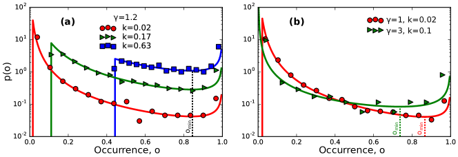
Supplementary Figure S7: Shape of the occurrence distribution for different values of $\gamma$ and $k$. a) For a given exponent $\gamma$ of the Zipf’s law, the value of the rescaling parameter $k$ determines the domain of possible occurrences and the actual fraction of core and rare components. b) The minimum position $o_{min}$ and the steepness of the decay of rare components are instead only a function of $\gamma$.

References

- Altmann and Gerlach (2016) E. G. Altmann and M. Gerlach, Statistical Laws in Linguistics (Springer International Publishing, Cham, 2016), pp. 7–26, ISBN 978-3-319-24403-7.
- Koonin (2011) E. V. Koonin, PLoS Comput. Biol. 7, e1002173 (2011).
- Cosentino Lagomarsino et al. (2009) M. Cosentino Lagomarsino, A. L. Sellerio, P. D. Heijning, and B. Bassetti, Genome Biol. 10, R12 (2009).
- Zipf (1935) G. K. Zipf, The Psychobiology of Language (Houghton-Mifflin, New York, NY, USA, 1935).
- Zanette and Montemurro (2005) D. Zanette and M. Montemurro, J. Quant. Ling. 12, 29 (2005).
- Newman (2005) M. E. J. Newman, Contemp. Phys. 46, 323 (2005).
- Lü et al. (2010) L. Lü, Z.-K. Zhang, and T. Zhou, PLoS One 5, e14139 (2010).
- Eliazar (2011) I. Eliazar, Physica A 390, 3189 (2011).
- Font-Clos and Corral (2015) F. Font-Clos and Á. Corral, Phys. Rev. Lett. 114, 238701 (2015).
- Huynen and van Nimwegen (1998) M. A. Huynen and E. van Nimwegen, Mol. Biol. Evol. 15, 583 (1998).
- Qian et al. (2001) J. Qian, N. M. Luscombe, and M. Gerstein, J. Mol. Biol. 313, 673 (2001).
- Karev et al. (2002) G. P. Karev, Y. I. Wolf, A. Y. Rzhetsky, F. S. Berezovskaya, and E. V. Koonin, BMC Evol. Biol. 2, 18 (2002).
- Karev et al. (2003) G. P. Karev, Y. I. Wolf, and E. V. Koonin, Bioinformatics 19, 1889 (2003).
- Mandelbrot (1953) B. Mandelbrot, Communication Theory 84, 486 (1953).
- i Cancho and Solé (2003) R. F. i Cancho and R. V. Solé, Proc. Natl. Acad. Sci. U.S.A. 100, 788 (2003).
- Simon (1955) H. A. Simon, Biometrika 42, 425 (1955).
- Gerlach and Altmann (2013) M. Gerlach and E. G. Altmann, Phys. Rev. X 3, 021006 (2013).
- Baek et al. (2011) S. K. Baek, S. Bernhardsson, and P. Minnhagen, New J. Phys. 13, 043004 (2011).
- Pang and Maslov (2013) T. Y. Pang and S. Maslov, Proc. Natl. Acad. Sci. U.S.A. 110, 6235 (2013).
- Touchon et al. (2009) M. Touchon, C. Hoede, O. Tenaillon, V. Barbe, S. Baeriswyl, P. Bidet, E. Bingen, S. Bonacorsi, C. Bouchier, O. Bouvet, et al., PLoS Genet. 5, e1000344 (2009).
- Koonin and Wolf (2008) E. V. Koonin and Y. I. Wolf, Nucleic Acids Res. 36, 6688 (2008).
- Haegeman and Weitz (2012) B. Haegeman and J. S. Weitz, BMC Genomics 13, 196 (2012).
- Lobkovsky et al. (2013) A. E. Lobkovsky, Y. I. Wolf, and E. V. Koonin, Genome Biol. Evol. 5, 233 (2013).
- Baumdicker et al. (2012) F. Baumdicker, W. R. Hess, and P. Pfaffelhuber, Genome Biol. Evol. 4, 443 (2012).
- Collins and Higgs (2012) R. E. Collins and P. G. Higgs, Mol. Biol. Evol. 29, 3413 (2012).
- Wilson et al. (2007) D. Wilson, M. Madera, C. Vogel, C. Chothia, and J. Gough, Nucleic Acids Res. 35, D308 (2007).
- Orengo and Thornton (2005) C. A. Orengo and J. M. Thornton, Annu. Rev. Biochem. 74, 867 (2005).
- Vogel and Chothia (2006) C. Vogel and C. Chothia, PLoS Comput. Biol. 2, e48 (2006).
- van Leijenhorst and Van der Weide (2005) D. C. van Leijenhorst and T. P. Van der Weide, Inform. Sci. 170, 263 (2005).
- Petersen et al. (2012) A. M. Petersen, J. N. Tenenbaum, S. Havlin, H. E. Stanley, and M. Perc, Sci. Rep. 2, 943 (2012).
- Lobkovsky et al. (2014) A. E. Lobkovsky, Y. I. Wolf, and E. V. Koonin, BMC Genomics 15, S14 (2014).
- Soucy et al. (2015) S. M. Soucy, J. Huang, and J. P. Gogarten, Nat. Rev. Genet. 16, 472 (2015).
- Dixit et al. (2015) P. D. Dixit, T. Yau Pang, F. W. Studier, and S. Maslov, Proc. Natl. Acad. Sci. U.S.A. 112, 9070 (2015).
- van Nimwegen (2003) E. van Nimwegen, Trends Genet. 19, 479 (2003).
- Molina and van Nimwegen (2009) N. Molina and E. van Nimwegen, Trends Genet. 25, 243 (2009).
- Maslov et al. (2009) S. Maslov, S. Krishna, T. Y. Pang, and K. Sneppen, Proc. Natl. Acad. Sci. U.S.A. 106, 9743 (2009).
- Grilli et al. (2011) J. Grilli, B. Bassetti, S. Maslov, and M. Cosentino Lagomarsino, Nucleic Acids Res. 40, 530 (2011).
- Mitzenmacher (2004) M. Mitzenmacher, Internet Mathematics 1, 226 (2004).
- Koonin (2003) E. V. Koonin, Nat. Rev. Microbiol. 1, 127 (2003).
- Heaps (1978) H. S. Heaps, Information retrieval: Computational and theoretical aspects (Academic Press, Inc., 1978).
- Hubbell (2001) S. P. Hubbell, The Unified Neutral Theory of Biodiversity and Biogeography (MPB-32) (Princeton University Press, 2001).
- Holovatch et al. (2017) Y. Holovatch, R. Kenna, and S. Thurner, Eur. J. Phys. 38, 023002 (2017).
- Lapierre and Gogarten (2009) P. Lapierre and J. P. Gogarten, Trends Genet. 25, 107 (2009).
- Azaele et al. (2016) S. Azaele, S. Suweis, J. Grilli, I. Volkov, J. R. Banavar, and A. Maritan, Rev. Mod. Phys. 88, 035003 (2016).
- Grilli et al. (2014) J. Grilli, M. Romano, F. Bassetti, and M. Cosentino Lagomarsino, Nucleic Acids Res. 42, 6850 (2014).