Learning Sparse Representations in Reinforcement Learning with Sparse Coding

Abstract

A variety of representation learning approaches have been investigated for reinforcement learning; much less attention, however, has been given to investigating the utility of sparse coding. Outside of reinforcement learning, sparse coding representations have been widely used, with non-convex objectives that result in discriminative representations. In this work, we develop a supervised sparse coding objective for policy evaluation. Despite the non-convexity of this objective, we prove that all local minima are global minima, making the approach amenable to simple optimization strategies. We empirically show that it is key to use a supervised objective, rather than the more straightforward unsupervised sparse coding approach. We compare the learned representations to a canonical fixed sparse representation, called tile-coding, demonstrating that the sparse coding representation outperforms a wide variety of tile-coding representations.

1 Introduction

For tasks with large state or action spaces, where tabular representations are not feasible, reinforcement learning algorithms typically rely on function approximation. Whether they are learning the value function, policy or models, the success of function approximation techniques hinges on the quality of the representation. Typically, representations are hand-crafted, with some common representations including tile-coding, radial basis functions, polynomial basis functions and Fourier basis functions  (Sutton, 1996; Konidaris et al., 2011). Automating feature discovery, however, alleviates this burden and has the potential to significantly improve learning.

Representation learning techniques in reinforcement learning have typically drawn on the large literature in unsupervised and supervised learning. Common approaches include feature selection, including $\ell_{1}$ regularization on the value function parameters (Loth et al., 2007; Kolter and Ng, 2009; Nguyen et al., 2013) and matching pursuit (Parr et al., 2008; Painter-Wakefield and Parr, 2012); basis-function adaptation approaches (Menache et al., 2005; Whiteson et al., 2007); instance-based approaches, such as locally weighted regression (Atkeson and Morimoto, 2003), sparse distributed memories (Ratitch and Precup, 2004), proto-value functions (Mahadevan and Maggioni, 2007) and manifold learning techniques (Mahadevan, 2009); and neural network approaches, including more standard feedforward neural networks (Coulom, 2002; Riedmiller, 2005; Mnih et al., 2015) as well as random representations (Sutton and Whitehead, 1993), linear threshold unit search (Sutton and Barto, 2013), and evolutionary algorithms like NEAT (Stanley and Miikkulainen, 2002).

Surprisingly, however, there has been little investigation into using sparse coding for reinforcement learning. Sparse coding approaches have been developed to learn MDP models for transfer learning (Ammar et al., 2012); outside this work, however, little has been explored. Nonetheless, such sparse coding representations have several advantages, including that they naturally enable local models, are computationally efficient to use, are much simpler to train than more complicated models such as neural networks and are biologically motivated by the observed representation in the mammalian cortex (Olshausen and Field, 1997).

In this work, we develop a principled sparse coding objective for policy evaluation. In particular, we formulate a joint optimization over the basis and the value function parameters, to provide a supervised sparse coding objective where the basis is informed by its utility for prediction. We highlight the importance of using the Bellman error or mean-squared return error for this objective, and discuss how the projected Bellman error is not suitable. We then show that, despite being a nonconvex objective, all local minima are global minima, under minimal conditions. We avoid the need for careful initialization strategies needed for previous optimality results for sparse coding (Agarwal et al., 2014; Arora et al., 2015), using recent results for more general dictionary learning settings (Haeffele and Vidal, 2015; Le and White, 2017), particularly by extending beyond smooth regularizers using $\Gamma$-convergence. Using this insight, we provide a simple alternating proximal gradient algorithm and demonstrate the utility of learning supervised sparse coding representations versus unsupervised sparse coding and a variety of tile-coding representations.

2 Background

In reinforcement learning, an agent interacts with its environment, receiving observations and selecting actions to maximize a scalar reward signal provided by the environment. This interaction is usually modeled by a Markov decision process (MDP). An MDP consists of $(\mathcal{S},\mathcal{A},P,R)$ where $\mathcal{S}$ is the set of states; $\mathcal{A}$ is a finite set of actions; $P:\mathcal{S}\times\mathcal{A}\times\mathcal{S}\rightarrow[0,1]$, the transition function, which describes the probability of reaching a state $s^{\prime}$ from a given state and action $(s,a)$; and finally the reward function $R:\mathcal{S}\times\mathcal{A}\times\mathcal{S}\rightarrow{\mathbb{R}}$, which returns a scalar value for transitioning from state-action $(s,a)$ to state $s^{\prime}$. The state of the environment is said to be Markov if $Pr(s_{t+1}|s_{t},a_{t})=Pr(s_{t+1}|s_{t},a_{t},\dots,s_{0},a_{0})$.

One important goal in reinforcement learning is policy evaluation: learning the value function for a policy. A value function $\mathbf{V}^{\pi}:\mathcal{S}\rightarrow{\mathbb{R}}$ approximates the expected return. The return $G_{t}$ from a state $s_{t}$ is the total discounted future reward, discounted by $\gamma\in[0,1)$, for following policy $\pi:\mathcal{S}\times\mathcal{A}\rightarrow[0,1]$

$$G_{t} =\sum_{i=0}^{\infty}\gamma^{i}R_{t+1+i}=R_{t+1}+\gamma G_{t+1}$$

where $\mathbf{V}^{\pi}(s_{t})$ is the expectation of this return from state $s_{t}$. This value function can also be thought of as a vector of values $\mathbf{V}^{\pi}\in{\mathbb{R}}^{|\mathcal{S}|}$ satisfying the Bellman equation

$$\mathbf{V}^{\pi} =\mathbf{r}^{\pi}+\gamma\mathbf{P}^{\pi}\mathbf{V}^{\pi}$$ (1)

$$\text{where }\ \ \mathbf{P}^{\pi}(s,s^{\prime}) =\sum_{a\in\mathcal{A}}\pi(s,a)P(s,a,s^{\prime})$$

$$\mathbf{r}^{\pi}(s) =\sum_{a\in\mathcal{A}}\pi(s,a)\sum_{s^{\prime}\in\mathcal{S}}P(s,a,s^{\prime})R(s,a,s^{\prime})$$

Given the reward function and transition probabilities, the solution can be analytically obtained: $\mathbf{V}^{\pi}=(\mathbf{I}-\gamma\mathbf{P}^{\pi})^{-1}\mathbf{r}^{\pi}$.

In practice, however, we likely have a prohibitively large state space. The typical strategy in this setting is to use function approximation to learn $\mathbf{V}^{\pi}(s)$ from a trajectory of samples: a sequence of states, actions, and rewards $s_{0}$, $a_{0}$, $r_{0}$, $s_{1}$, $a_{1}$, $r_{1}$, $s_{2}$, $r_{2}$, $a_{2}\ldots$, where $s_{0}$ is drawn from the start-state distribution, $s_{t+1}\sim P(\cdot|s_{t},a_{t})$ and $a_{t}\sim\pi(\cdot|s_{t})$. Commonly, a linear function is assumed, $\mathbf{V}^{\pi}(s)\approx\boldsymbol{\phi}(s)^{\top}\mathbf{w}$ for $\mathbf{w}\in{\mathbb{R}}^{k}$ a parameter vector and $\boldsymbol{\phi}:\mathcal{S}\rightarrow{\mathbb{R}}^{k}$ a feature function describing states. With this approximation, however, typically we can no longer satisfy the Bellman equation in (1), because there may not exist a ${{\mathbf{w}}}$ such that $\boldsymbol{\Phi}\mathbf{w}$ equals $\mathbf{r}^{\pi}+\gamma\mathbf{P}^{\pi}\boldsymbol{\Phi}\mathbf{w}$ for $\boldsymbol{\Phi}\in{\mathbb{R}}^{|\mathcal{S}|\times k}$. Instead, we focus on minimizing the error to the true value function.

Reinforcement learning algorithms, such as temporal difference learning and residual gradient, therefore focus on finding an approximate solution to the Bellman equation, despite this representation issue. The quality of the representation is critical to accurately approximating $\mathbf{V}^{\pi}$ with $\boldsymbol{\Phi}{{\mathbf{w}}}$, but also balancing compactness of the representation and speed of learning. Sparse coding, and sparse representations, have proven successful in machine learning and in reinforcement learning, particularly as fixed bases, such as tile coding, radial basis functions and other kernel representations. A natural goal, therefore, and the one we explore in this work, is to investigate learning these sparse representations automatically.

3 Sparse Coding for Reinforcement Learning

In this section, we formalize sparse coding for reinforcement learning as a joint optimization over the value function parameters and the representation. We introduce the true objective over all states, and then move to the sampled objective for the algorithm in the next section.

We begin by formalizing the representation learning component. Many unsupervised representation learning approaches consist of factorizing input observations $\mathbf{X}\!\in\!{\mathbb{R}}^{|\mathcal{S}|\times d}$ into a basis dictionary $\mathbf{B}\!\in\!{\mathbb{R}}^{k\times d}$ and new representation $\boldsymbol{\Phi}\in{\mathbb{R}}^{|\mathcal{S}|\times k}$. The rows of $\mathbf{B}$ form a set of bases, with columns in $\boldsymbol{\Phi}$ weighting amongst those bases for each observation (column) in $\mathbf{X}$. Though simple, this approach encompasses a broad range of models, including PCA, CCA, ISOMAP, locally linear embeddings and sparse coding (Singh and Gordon, 2008; Le and White, 2017). The (unsupervised) sparse coding objective is (Aharon et al., 2006)

$$\min_{\boldsymbol{\Phi}\in{\mathbb{R}}^{|\mathcal{S}|\times k},\mathbf{B}\in{\mathbb{R}}^{k\times d}}\|\boldsymbol{\Phi}\mathbf{B}-\mathbf{X}\|_{D}^{2}+\beta_{B}\|\mathbf{B}\|_{F}^{2}+\beta_{\phi}\|\boldsymbol{\Phi}\|_{D,1}$$

where $\|\mathbf{Y}\|_{F}^{2}=\sum_{ij}\mathbf{Y}_{ij}^{2}$ is the squared Frobenius norm; $\mathbf{B}\in{\mathbb{R}}^{k\times d}$ is a learned basis dictionary; $\beta_{B},\beta_{\phi}>0$ determine the magnitudes of the regularizers; $\mathbf{D}\in[0,1]^{|\mathcal{S}|\times|\mathcal{S}|}$ is a diagonal matrix giving a distribution over states, corresponding to the stationary distribution of the policy $d^{\pi}:\mathcal{S}\rightarrow[0,1]$; and $||{{\mathbf{z}}}||^{2}_{D}={{\mathbf{z}}}^{\top}\mathbf{D}{{\mathbf{z}}}$ is a weighted norm. The reconstruction error

$$\|\boldsymbol{\Phi}\mathbf{B}-\mathbf{X}\|_{D}^{2}=\sum_{s\in\mathcal{S}}d^{\pi}(s)\|\boldsymbol{\Phi}(s,:)\mathbf{B}-\mathbf{X}(s,:)\|_{2}^{2}$$

is weighted by the stationary distribution $d^{\pi}$ because states are observed with frequency indicated by $d^{\pi}$. The weighted $\ell_{1}$

$$\|\boldsymbol{\Phi}\|_{D,1}=\sum_{s\in\mathcal{S}}d^{\pi}(s)\sum_{j=1}^{k}|\boldsymbol{\Phi}(s,j)|$$

promotes sparsity on the entries of $\boldsymbol{\Phi}$, preferring entries in $\boldsymbol{\Phi}$ to be entirely pushed to zero rather than spreading magnitude across all of $\boldsymbol{\Phi}$. The Frobenius norm regularizer on $\mathbf{B}$ ensures that $\mathbf{B}$ does not become too large. Without this regularizer, all magnitude can be shifted to $\mathbf{B}$, producing the same $\boldsymbol{\Phi}\mathbf{B}$, but pushing $\|\boldsymbol{\Phi}\|_{D,1}$ to zero and nullifying the utility of its regularizer. Optimizing this sparse coding objective would select a sparse representation $\boldsymbol{\phi}$ for each observation ${{\mathbf{x}}}$ such that $\boldsymbol{\phi}\mathbf{B}$ approximately reconstructs ${{\mathbf{x}}}$.

Further, however, we would like to learn a new representation that is also optimized towards approximating the value function. Towards this aim, we need to jointly learn $\boldsymbol{\Phi}$ and ${{\mathbf{w}}}$, where $\boldsymbol{\Phi}{{\mathbf{w}}}$ provides the approximate value function. In this way, the optimization must balance between accurately recreating $\mathbf{X}$ and approximating the value function $\boldsymbol{\Phi}{{\mathbf{w}}}$. For this, we must choose an objective for learning ${{\mathbf{w}}}$.

We consider two types of objectives: fixed-point objectives and squared-error objectives. Two common fixed-point objectives are the mean-squared Bellman error (MSBE), also called the Bellman residual (Baird, 1995)

$$\|\boldsymbol{\Phi}\mathbf{w}-(\mathbf{r}^{\pi}+\gamma\mathbf{P}^{\pi}\boldsymbol{\Phi}\mathbf{w})\|^{2}_{D}$$

and mean-squared projected BE (MSPBE) (Sutton et al., 2009)

$$\|\boldsymbol{\Phi}\mathbf{w}-\Pi(\mathbf{r}^{\pi}+\gamma\mathbf{P}^{\pi}\boldsymbol{\Phi}\mathbf{w})\|^{2}_{D}$$

where $\mathbf{D}\in[0,1]^{|\mathcal{S}|\times|\mathcal{S}|}$ is a diagonal matrix giving a distribution over states, corresponding to the stationary distribution of the policy; $||{{\mathbf{z}}}||^{2}_{D}={{\mathbf{z}}}^{\top}\mathbf{D}{{\mathbf{z}}}$ is a weighted norm; and the projection matrix for linear value functions is $\Pi=\boldsymbol{\Phi}(\boldsymbol{\Phi}^{\top}\mathbf{D}\boldsymbol{\Phi})^{-1}\boldsymbol{\Phi}^{\top}\mathbf{D}$. The family of TD algorithms converge to the minimum of the MSPBE, whereas residual gradient algorithms typically use the MSBE (see (Sun and Bagnell, 2015) for an overview). Both have useful properties (Scherrer, 2010), though arguably the MSPBE is more widely used.

There are also two alternative squared-error objectives, that do not correspond to fixed-point equations: the mean-squared return error (MSRE) and the Bellman error (BE). For a trajectory of samples $\{({{\mathbf{x}}}_{i},r_{i+1},{{\mathbf{x}}}_{i+1})\}_{i=0}^{t-1}$, BE is defined as

$$\sum_{i=0}^{t-1}\|r_{i+1}+\gamma\boldsymbol{\phi}_{i+1}^{\top}\mathbf{w}-\boldsymbol{\phi}_{i}^{\top}\mathbf{w}\|_{2}^{2}$$

and the MSRE as

$$\sum_{i=0}^{t-1}\|g_{i+1}-\boldsymbol{\phi}_{i}^{\top}\mathbf{w}\|_{2}^{2}$$

where $g_{i+1}=\sum_{j=i}^{t-1}\gamma^{j-i}r_{j+1}$ is a sample return. In expectation, these objectives are, respectively

$$\!\!\!\sum_{s\in\mathcal{S}}\!d^{\pi}\!(s)\mathbb{E}\!\!\left[\!\!\left(r(S_{t},A_{t},S_{t+1})\!+\!\gamma\boldsymbol{\phi}(S_{t+1})^{\top}\mathbf{w}-\boldsymbol{\phi}(S_{t})^{\top}\mathbf{w}\right)^{2}\!\!|S_{t}\!\!=\!\!s\right]$$

$$\!\!\!\sum_{s\in\mathcal{S}}\!d^{\pi}\!(s)\mathbb{E}\!\left[\!\!\left(\sum_{i=0}^{\infty}\gamma^{i}r(S_{t+i},A_{t+i},S_{t+1+i})-\boldsymbol{\phi}(s)^{\top}\mathbf{w}\right)^{2}\!\!\!\!|S_{t}\!\!=\!\!s\right]$$

where the expectation is w.r.t. the transition probabilities and taking actions according to policy $\pi$.

These differ from the fixed-point objectives because of the placement of the expectation. To see why, consider the MSBE and BE. The expected value of the BE is the expected squared error between the prediction from this state and the reward plus the value from a possible next state. The MSBE, on the other hand, is the squared error between the prediction from this state and the expected reward plus the expected value for the next state. Though the MSPBE and MSBE constitute the most common objectives chosen for reinforcement learning, these squared-error objectives have also been shown to be useful particularly for learning online (Sun and Bagnell, 2015).

For sparse coding, however, the MSPBE is not a suitable choice—compared to the MSBE, BE and MSRE—for two reasons. First, the MSBE, BE and MSRE are all convex in $\boldsymbol{\Phi}$, whereas the MSPBE is not. Second, because of the projection onto the space spanned by the features, the MSPBE can be solved with zero error for any features $\boldsymbol{\Phi}$. Therefore, because it does not inform the choice of $\boldsymbol{\Phi}$, the MSPBE produces a two stage approach, where features are learned in a completely unsupervised way and prediction performance does not influence $\boldsymbol{\Phi}$.

The final objective for loss $\textrm{L}(\boldsymbol{\Phi},\mathbf{w})$ set to either MSBE, BE or MSRE is

$$\min_{\mathbf{w}\in{\mathbb{R}}^{k},\boldsymbol{\Phi}\in{\mathbb{R}}^{|\mathcal{S}|\times k},\mathbf{B}\in{\mathbb{R}}^{k\times d}} \textrm{L}(\boldsymbol{\Phi},\mathbf{w})+\|\boldsymbol{\Phi}\mathbf{B}-\mathbf{X}\|_{D}^{2}$$ (2)

$$+\beta_{w}\|\mathbf{w}\|_{2}^{2}+\beta_{B}\|\mathbf{B}\|_{F}^{2}+\beta_{\phi}\|\boldsymbol{\Phi}\|_{D,1}$$

4 Algorithm for Sparse Coding

We now derive the algorithm for sparse coding for policy evaluation: SCoPE. We generically consider either the BE or MSRE. For a trajectory of samples $\{({{\mathbf{x}}}_{i},r_{i+1},{{\mathbf{x}}}_{i+1})\}_{i=0}^{t-1}$, the objective is

$$\min_{\mathbf{w}\in{\mathbb{R}}^{k},\boldsymbol{\Phi}\in{\mathbb{R}}^{t+1\times k},\mathbf{B}\in{\mathbb{R}}^{k\times d}}\frac{1}{t}\sum_{i=0}^{t-1}(y_{i}+\bar{\gamma}\boldsymbol{\phi}_{i+1}^{\top}\mathbf{w}-\boldsymbol{\phi}_{i}^{\top}\mathbf{w})^{2}$$ (3)

$$\!\!+\frac{1}{t}\!\sum_{i=0}^{t}\!\|\boldsymbol{\phi}_{i}\mathbf{B}-{{\mathbf{x}}}_{i}\|_{2}^{2}+\!\beta_{B}\|\mathbf{B}\|_{F}^{2}+\!\beta_{w}\|\mathbf{w}\|_{2}^{2}\!+\!\frac{\beta_{\phi}}{t}\sum_{i=0}^{t}\|\boldsymbol{\phi}_{i}\|^{p}_{1}.$$

for BE, $y_{i}=r_{i+1}$ and $\bar{\gamma}=\gamma$ and for MSRE, $y_{i}=\sum_{j=i}^{t}\gamma^{j-i}r_{j+1}$ and $\bar{\gamma}=0$. We consider two possible powers for the $\ell_{1}$ norm $p=1$ or $2$, where the theory relies on using $p=2$, but in practice we find they perform equivalently and $p=1$ provides a slightly simpler optimization. The loss is averaged by $t$, to obtain a sample average, which in the limit converges to the expected value under $d^{\pi}$. This averaged loss is also more scale-invariant—in terms of the numbers of samples—to the choice of regularization parameters.

SCoPE consists of alternating amongst these three variables, $\mathbf{B},\mathbf{w}$ and $\boldsymbol{\Phi}$, with a proximal gradient update for the non-differentiable $\ell_{1}$ norm. The loss in terms of $\mathbf{B}$ and $\mathbf{w}$ is differentiable; to solve for $\mathbf{B}$ (or $\mathbf{w}$) with the other variables fixed, we can simply used gradient descent. To solve for $\boldsymbol{\Phi}$ with the $\mathbf{B}$ and $\mathbf{w}$ fixed, however, we cannot use a standard gradient descent update because the $\ell_{1}$ regularizer is non-differentiable. The proximal update consists of stepping in the direction of the gradient for the smooth component of the objective—which is differentiable—and then projecting back to a sparse solution using the proximal operator: a soft thresholding operator. The convergence of this alternating minimization follows from results on block coordinate descent for non-smooth regularizers (Xu and Yin, 2013).

To apply the standard proximal operator for the $\ell_{1}$ regularizer, we need to compute an upper bound on the Lipschitz constant for this objective. The upper bound is $2(1+\bar{\gamma}^{2})\|\mathbf{w}\|_{2}^{2}+2\|\mathbf{B}\|_{sp}^{2}$, computed by finding the maximum singular value of the Hessian of the objective w.r.t. $\boldsymbol{\phi}_{i}$ for each $i$. We will provide additional details for this calculation, and implementation details, in a supplement.

4.1 Local Minima Are Global Minima

In this section, we show that despite nonconvexity, the objective for SCoPE has the nice property that all local minima are in fact global minima. Consequently, though there may be many different local minima, they are in fact equivalent in terms of the objective. This result justifies a simple alternating minimization scheme, where convergence to local minima ensures an optimal solution is obtained.

We need the following technical assumption. It is guaranteed to be true for a sufficiently large $k\leq t$ (see Haeffele and Vidal (2015); Le and White (2017)).

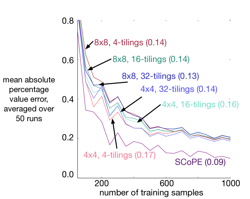
(a) Mountain Car

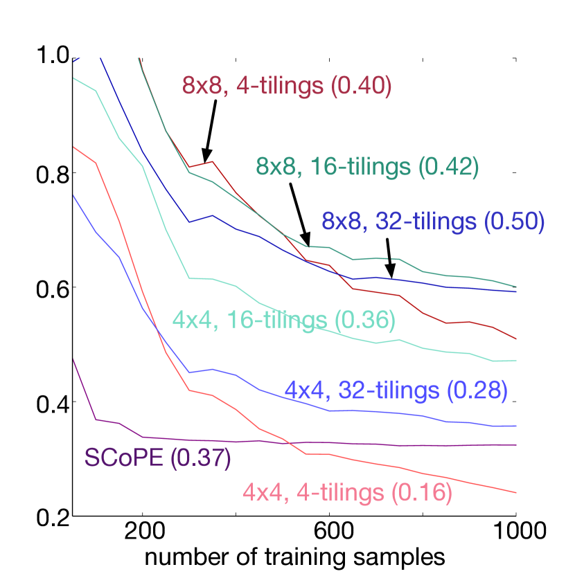
(b) Puddle World

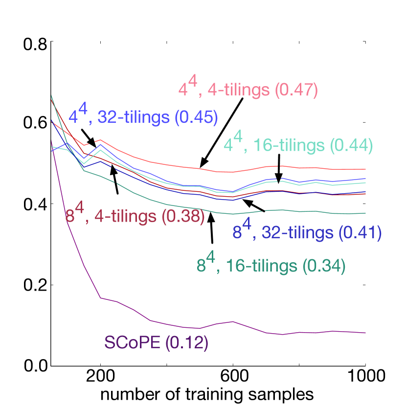
(c) Acrobot

Figure 1: Learning curves for SCoPE versus a variety of tile coding representations in three domains. The graphs depict early learning; the numbers in brackets correspond to final error, after 5000 samples. Because errors are sampled every 50 samples, and because MSRE is used for optimization, the lines have an irregular pattern. The differences are nonetheless statistically significant, with an average over 50 runs, and so the small standard error bars are omitted. SCoPE outperforms the best of the TC representations in Mountain Car and Acrobot  using a more compact sparse representation; in Puddle World, it performs more poorly, which we discuss further in the text. The larger TC representations likely perform poorly due to hashing.

Assumption 1 For the given $k\geq d$, the following function is convex in $\mathbf{Z}\in{\mathbb{R}}^{t+1\times d+1}$

$$\min_{\boldsymbol{\Phi},\mathbf{B},\mathbf{w},\mathbf{Z}=\boldsymbol{\Phi}[\negthinspace\begin{smallmatrix}\mathbf{B}\ \mathbf{w}\end{smallmatrix}]}\beta_{B}\|\mathbf{B}\|_{F}^{2}+\beta_{w}\|\mathbf{w}\|_{2}^{2}+\frac{\beta_{\phi}}{t}\sum_{i=0}^{t}\|\boldsymbol{\phi}_{i}\|^{2}_{1}$$

Theorem 1 (Landscape of the SCoPE objective).

For the objective in equation (3) with $p=2$,

1. under Assumption 1, all full-rank local minima are global minima; and

2. if a local minimum $(\boldsymbol{\Phi},\mathbf{B},\mathbf{w})$ has $\boldsymbol{\Phi}_{:i}={{\mathbf{0}}}$ (i.e., a zero column) and $\mathbf{w}_{i}=0$, $\mathbf{B}_{i:}={{\mathbf{0}}}$ (i.e., a zero row) for some $1\leq i\leq k$, then it is a global minimum.

Proof.

For the first statement, we construct a limit of twice-differentiable functions $f_{n}$ that $\Gamma$-converge to the SCoPE objective $f$. With this, we can then show that all minimizers of the sequence converge to minimizers of $f$, and vice-versa (Braides, 2013). Because all local minimizers of the twice-differentiable functions $f_{n}$ are global minimizers from (Le and White, 2017, Theorem 10), we can conclude that all corresponding minimizers of $f$ are global minimizers.

We use the pseudo-Huber loss (Fountoulakis and Gondzio, 2013), which is twice-differentiable approximation to the absolute value: $|x|_{\mu}=\sqrt{\mu^{2}+x^{2}}-\mu$. Let $\boldsymbol{\theta}=(\boldsymbol{\Phi},\mathbf{B},\mathbf{w})$. The sequence of functions $f_{n}$ are defined with $\mu_{n}=1/n$, as

$$f_{n}(\boldsymbol{\theta})=L(\boldsymbol{\theta})+\frac{\beta_{\phi}}{t}\sum_{ij}\sqrt{\mu_{n}^{2}+\boldsymbol{\Phi}_{ij}^{2}}-\mu_{n}$$

where $L(\boldsymbol{\theta})$ equals the equation in (3), but without the $\ell_{1}^{2}$ regularizer on $\boldsymbol{\Phi}$.

Part 1: All local minima of $f_{n}$ for all $n$ are global minima. To show this, we show each $f_{n}$ satisfies the conditions of (Le and White, 2017, Theorem 10 and Proposition 11).

Part 1.1 We can rewrite the loss in terms of $\boldsymbol{\Phi}[\negthinspace\begin{smallmatrix}\mathbf{B}\ \mathbf{w}\end{smallmatrix}]$

$$\!\!\!\!\frac{1}{t}\sum_{i=0}^{t-1}\|y_{i}+\bar{\gamma}\boldsymbol{\phi}_{i+1}^{\top}\mathbf{w}-\boldsymbol{\phi}_{i}^{\top}\mathbf{w}\|_{2}^{2}+\frac{1}{t}\sum_{i=0}^{t}\|\boldsymbol{\phi}_{i}\mathbf{B}-{{\mathbf{x}}}_{i}\|_{2}^{2}$$

$$\!\!\!\!=\frac{1}{t}\left\|\mathbf{X}-\boldsymbol{\Phi}\mathbf{B}\right\|_{2}^{2}\!+\!\frac{1}{t}\left\|\mathbf{y}-\left(\mathbf{I}_{0:t-1}\!-\!\bar{\gamma}\mathbf{I}_{1:t}\right)\boldsymbol{\Phi}\mathbf{w}\right\|_{2}^{2}$$ (4)

where $\mathbf{I}_{1:t}\in{\mathbb{R}}^{t\times t+1}$ a diagonal matrix of all ones with the first diagonal entry set to zero, and $\mathbf{I}_{0:t-1}$ with the last diagonal entry set to zero. This loss is convex in the joint variable $\boldsymbol{\Phi}[\negthinspace\begin{smallmatrix}\mathbf{B}\ \mathbf{w}\end{smallmatrix}]$ because equation (4) is the composition of a convex function (squared norm) and an affine function (multiplication by $\bar{\gamma}\mathbf{I}_{1:t}-\mathbf{I}_{0:t-1}$ and addition of $\mathbf{y}$).

Part 1.2 The regularizer on $[\negthinspace\begin{smallmatrix}\mathbf{B}\ \mathbf{w}\end{smallmatrix}]$ must be a weighted Frobenius norm, with weightings on each column; here, we have weighting using regularization parameters $\beta_{B}$ for the first $d$ columns (corresponding to $\mathbf{B}$) and regularization parameter $\beta_{w}$ for the last column (corresponding to $\mathbf{w}$).

Part 1.3 The inner dimension $k>d$, which is true by assumption and the common setting for sparse coding.

Part 1.4 The pseudo-Huber loss, on the columns of $\boldsymbol{\Phi}$, is convex, centered and twice-differentiable.

Part 2: The sequence $f_{n}$ converges uniformly to $f$. To see why, recall the definition of uniform convergence. A sequence of functions $\{f_{n}\}$ is uniformly convergent with limit $f$ if for every $\epsilon>0$, there exists $N\in{\mathbb{N}}$ such that for all $\boldsymbol{\theta}\in\Theta$ all $n\geq N$, $|f_{n}(\boldsymbol{\theta})-f(\boldsymbol{\theta})|<\epsilon$. Further recall that for any complete metric space, if $f_{n}$ is uniformly Cauchy, then it is uniformly convergent. The sequence is uniformly Cauchy if for all $n,m\geq N$, $|f_{n}(\boldsymbol{\theta})-f_{m}(\boldsymbol{\theta})|<\epsilon$. Take any $\epsilon>0$ and let $N=\lceil\tfrac{4k(t+1)\beta_{\phi}}{t\epsilon}\rceil$. Then

$$|f_{n}(\boldsymbol{\theta})-f_{m}(\boldsymbol{\theta})|$$

$$=\frac{\beta_{\phi}}{t}\left|\!\!\left(\!\!\sum_{ij}\sqrt{\mu_{n}^{2}+\boldsymbol{\Phi}_{ij}^{2}}-\mu_{n}\right)\!\!-\!\!\left(\!\!\sum_{ij}\sqrt{\mu_{m}^{2}+\boldsymbol{\Phi}_{ij}^{2}}-\mu_{m}\right)\!\!\right|$$

$$\leq\frac{\beta_{\phi}}{t}\sum_{ij}\left(\left|\sqrt{\mu_{n}^{2}+\boldsymbol{\Phi}_{ij}^{2}}-\sqrt{\mu_{m}^{2}+\boldsymbol{\Phi}_{ij}^{2}}\right|+\left|\mu_{n}-\mu_{m}\right|\right)$$

The upper bound of the first component is maximized when $\boldsymbol{\Phi}_{ij}=0$, and so we get

$$\!\!|f_{n}(\boldsymbol{\theta})\!-\!f_{m}(\boldsymbol{\theta})| \!\leq\!\tfrac{2k(t+1)\beta_{\phi}}{t}\left|\mu_{n}\!-\!\mu_{m}\right|\!\leq\!\tfrac{2k(t+1)\beta_{\phi}}{t}\left|\tfrac{1}{n}\!-\!\tfrac{1}{m}\right|$$

$$\!\leq\!\tfrac{4k(t+1)\beta_{\phi}}{tN}\leq\epsilon.$$

Part 3: Asymptotic equivalence of minimizers of $f_{n}$ and $f$. Because $f$ is continuous, and so lower semi-continuous, and $f_{n}$ uniformly converges to $f$, we know that $f_{n}$ $\Gamma$-converges to $f$: $f_{n}\overset{\Gamma}{\rightarrow}f$ Braides (2013).

By the fundamental theorem of $\Gamma$-convergence, if the $\{f_{n}\}$ is an equi-coercive family of functions, then the minimizers of $f_{n}$ converge to minimizers of $f$. A sequence of functions $\{f_{n}\}$ is equi-coercive iff there exists a lower semi-continuous coercive function $\psi:\Theta\rightarrow{\mathbb{R}}\cup\{-\infty,\infty\}$ such that $f_{n}\geq\psi$ on $\Theta$ for every $n\in{\mathbb{N}}$ (Dal Maso, 2012, Proposition 7.7). A function is coercive if $\psi(\theta)\rightarrow\infty$ as $\|\theta\|\rightarrow\infty$. For $\psi(\theta)=L(\boldsymbol{\theta})$, it is clear that $\psi$ is coercive, as well as lower semi-continuous (since it is continuous). Further, $f_{n}(\boldsymbol{\theta})\geq L(\boldsymbol{\theta})=\psi(\boldsymbol{\theta})$, because the regularizer on $\boldsymbol{\Phi}$ is non-negative. Therefore, the family $\{f_{n}\}$ is equi-coercive, and so the minimizers of $f_{n}$ converge to minimizers of $f$.

For the other direction, if a local minimum $\boldsymbol{\theta}$ of $f$ is an isolated local minimum, then there exists a sequence $\boldsymbol{\theta}_{n}\rightarrow\boldsymbol{\theta}$ with $\boldsymbol{\theta}_{n}$ a local minimizer of $f_{n}$ for $\mu_{n}$ sufficiently small (Braides, 2013, Theorem 5.1). Because we have Frobenius norm regularizers on $\mathbf{B},\mathbf{w}$, which are strongly convex, the objective is strictly convex with respect to $\mathbf{B},\mathbf{w}$. Further, because $\mathbf{X}$ is full rank, $\|\boldsymbol{\Phi}\mathbf{B}-\mathbf{X}\|_{F}^{2}$ is a strictly convex function with respect to $\boldsymbol{\Phi}$. Therefore, locally the objective is strictly convex with respect to $\boldsymbol{\theta}$. We therefore know that local minima of $f$ are isolated, and so there exists an $N$ such that for all $n>N$, $\boldsymbol{\theta}_{n}$ are local minimizers of $f_{n}$. Since these local minimizers are global minimizers, and they converge to $\boldsymbol{\theta}$, this means $\boldsymbol{\theta}$ is a global minimum of $f$.

For the second statement, we use (Haeffele and Vidal, 2015, Theorem 15). Because we already showed above that our loss can be cast as factorization, it is clear our loss and regularizers are positively homogenous, of order 2. A minimum is guaranteed to exist for our objective, because the loss function is continuous, bounded below (by zero) and goes to infinity as the parameters go to $\pm\infty$. ∎

5 Experimental Results

We aim to address the question: can we learn useful representations using SCoPE? We therefore tackle the setting where the representation is first learned, and then used, to avoid conflating incremental estimation and the utility of the representation. We particularly aim to evaluate estimation accuracy, as well as qualitatively understanding the types of sparse representations learned by SCoPE.

Domains. We conducted experiments in three benchmark RL domains - Mountain Car, Puddle World and Acrobot (Sutton, 1996). All domains are episodic, with discount set to 1 until termination. The data in Mountain Car is generated using the standard energy-pumping policy policy with 10% randomness. The data in Puddle World is generated by a policy that chooses to go North with 50% probability, and East with 50% probability on each step, with the starting position in the lower-left corner of the grid, and the goal in the top-right corner. The data in Acrobot is generated by a near-optimal policy.

Evaluation. We measure value function estimation accuracy using mean absolute percentage value error (MAPVE), with rollouts to compute the true value estimates. $\text{MAPVE}=\frac{1}{t_{test}}\sum_{s\in X_{test}}\frac{|\hat{V}(s)-V^{*}(s)|}{|V^{*}(s)|}$, where $X_{test}$ is the set of test states, $t_{test}=5000$ is the number of samples in the test set, $\hat{V}(s)$ is the estimated value of state $s$ and $V^{*}(s)$ is the true value of state $s$ computed using extensive rollouts. Errors are averaged over 50 runs.

Algorithms. We compare to using several fixed tile-coding (TC) representations. TC uses overlapping grids on the observation space. It is a sparse representation that is well known to perform well for Mountain Car, Puddle World, and Acrobot. We varied the granularity of the grid-size N and number of tilings D, where $D$ is the number of active features for each observation. The grid is either N$\times$N for Mountain Car and Puddle World or N⁴ for Acrobot. We explore (D=4, N=4), (D=4,N=8), (D=16,N=4), (D=16,N=8), (D=32,N=4), (D=32,N=8); a grid size of 16 performed poorly, and so is omitted. For Mountain Car and Puddle World  the number of features respectively are 64, 256, 256, 1024, 512, 2048, then hashed to 1024 dimensions; for Acrobot, the number of features are 1024, 16384, 4096, 65536, 8192, 131072, then hashed to 4096. Both of these hashed sizes are much larger than our chosen $k=100$.

For consistency, once the SCoPE representation is learned, we use the same batch gradient descent update on the MSRE for all the algorithms, with line search to select step-sizes. The regularization weights $\beta_{B}$ are chosen from $\{1^{-5},\ldots,1^{-1},0\}$, based on lowest cumulative error. For convenience, $\beta_{w}$ is fixed to be the same as $\beta_{B}$. For learning the SCoPE representations, regularization parameters were chosen using 5-fold cross-validation on 5000 training samples, with $\beta_{\phi}=0.1$ fixed to give a reasonable level of sparsity. This data is only used to learn the representation; for the learning curves, the weights are learned from scratch in the same way they are learned for TC. The dimension $k=100$ is set to be smaller than for tile coding, to investigate if SCoPE can learn a more compact sparse representation. We tested unsupervised sparse coding, but the error was poor (approximately $10\times$ worse). We discuss the differences between the representations learned by supervised and unsupervised sparse coding below.

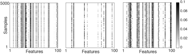
Figure 2: Learned representations $\boldsymbol{\Phi}$ for 5000 samples and $k=100$, respectively for SCoPE, unsupervised sparse coding, and non-negative unsupervised sparse coding, in Puddle World. The representations learned for Mountain Car and Acrobot have similar structure. The non-negative sparse coding has the additional constraint that each entry in $\boldsymbol{\Phi}$ is non-negative. The goal for this addition was to determine if further constraints could improve prediction accuracy for unsupervised sparse coding; though the representation qualitatively looks more reasonable, prediction performance remained poor.

Learning curves. We first demonstrate learning with increasing number of samples, in Figure 1. The weights are recomputed using the entire batch up to the given number of samples.

Across domains, SCoPE results in faster learning and, in Mountain Car and Acrobot, obtains lowest final error. Matching the performance of TC is meaningful, as TC is well-understood and optimized for these domains. For Acrobot, it’s clear a larger TC is needed resulting in relatively poor performance, whereas SCoPE can still perform well with a compact, learned sparse representation. These learning curves provide some insight that we can learn effective sparse representations with SCoPE, but also raise some questions. One issue is that SCoPE is not as effective in Puddle World as some of the TC representations, namely 4-4 and 16-4. The reason for this appears to be that we optimize MSRE to obtain the representation, which is a surrogate for the MAPVE. When measuring MSRE instead of MAPVE on the test data, SCoPE consistently outperforms TC. Optimizing both the representation and weights according to MSRE may have overfitting issues; extensions to MSBE or BE, or improvements in selecting regularization parameters, may alleviate this issue.

Learned representations. We also examine the learned representations, both for unsupervised sparse coding and SCoPE, shown in Figure 2. We draw two conclusions from these results: the structure in the observations is not sufficient for unsupervised sparse coding, and the combination of supervised and unsupervised losses sufficiently constrain the space to obtain discriminative representations. For these two-dimensional and four-dimensional observations, it is relatively easy to reconstruct the observations by using only a small subset of dictionary atoms (row vectors of $\mathbf{B}$ in equation (2)). The unsupervised representations, even with additional non-negativity constraints to narrow the search space, are less distributed, with darker and thicker blocks, and more frequently pick less features. For the supervised sparse coding representation, however, the sparsity pattern is smoother and more distributed: more features are selected by at least one sample, but the level of sparsity is similar. We further verified the utility of supervised sparse coding, by only optimizing the supervised loss (MSRE), without including the unsupervised loss; the resulting representations looked similar to the purely unsupervised representations. The combination of the two losses, therefore, much more effectively constrains or regularizes the space of feasible representations and improves discriminative power.

The learning demonstrated for SCoPE here is under ideal conditions. This was intentionally chosen to focus on the question: can we learn effective sparse representations using the SCoPE objective? With the promising results here, future work needs to investigate the utility of jointly estimating the representation and learning the value function, as well as providing incremental algorithms for learning the representations and setting the regularization parameters.

6 Conclusion

In this work, we investigated sparse coding for policy evaluation in reinforcement learning. We proposed a supervised sparse coding objective, for joint estimation of the dictionary, sparse representation and value function weights. We provided a simple algorithm that uses alternating minimization on these variables, and proved that this simple and easy-to-use approach is principled. We finally demonstrate results on three benchmark domains, Mountain Car, Puddle World and Acrobot, against a variety of configurations for tile coding.

This paper provides a new view of using dictionary learning techniques from machine learning in reinforcement learning. It lays a theoretical and empirical foundation for further investigating sparse coding, and other dictionary learning approaches, for policy evaluation and suggests that they show some promise. Formalizing representation learning as a dictionary learning problem facilitates extending recent and upcoming advances in unsupervised learning to the reinforcement learning setting. For example, though we considered a batch gradient descent approach for this first investigation, the sparse coding objective is amenable to incremental estimation, with several works investigating effective stochastic gradient descent algorithms (Mairal et al., 2009, 2010; Le and White, 2017). The generality of the approach and easy to understand optimization make it a promising direction for representation learning in reinforcement learning.

References

- Agarwal et al. [2014] Alekh Agarwal, Animashree Anandkumar, Prateek Jain, and Praneeth Netrapalli. Learning sparsely used overcomplete dictionaries via alternating minimization. In Ann. Conf. on Learning Theory, 2014.
- Aharon et al. [2006] Michal Aharon, Michael Elad, and Alfred Bruckstein. K-SVD: An Algorithm for Designing Overcomplete Dictionaries for Sparse Representation. IEEE Transactions on Signal Processing, 2006.
- Ammar et al. [2012] Haitham B Ammar, Karl Tuyls, Matthew E Taylor, Kurt Driessens, and Gerhard Weiss. Reinforcement learning transfer via sparse coding. In Inter. Conf. on Autonomous Agents and Multiagent Systems, 2012.
- Arora et al. [2015] Sanjeev Arora, Rong Ge, Tengyu Ma, and Ankur Moitra. Simple, efficient, and neural algorithms for sparse coding. arXiv:1503.00778v1 [cs.LG], 2015.
- Atkeson and Morimoto [2003] Christopher G Atkeson and Jun Morimoto. Nonparametric representation of policies and value functions: a trajectory-based approach. In Advances in Neural Information Processing Systems, 2003.
- Baird [1995] Leemon Baird. Residual algorithms: Reinforcement learning with function approximation. In Inter. Conf. on Mach. Learning, 1995.
- Bhatnagar et al. [2009] Shalabh Bhatnagar, Doina Precup, David Silver, Richard S Sutton, Hamid R Maei, and Csaba Szepesvári. Convergent temporal-difference learning with arbitrary smooth function approximation. In Advances in Neural Information Processing Systems, 2009.
- Braides [2013] Andrea Braides. Local minimization, variational evolution and -convergence. Lecture Notes in Mathematics, 2013.
- Coulom [2002] Rémi Coulom. Reinforcement learning using neural networks, with applications to motor control. PhD thesis, INPG, 2002.
- Dal Maso [2012] Gianni Dal Maso. An Introduction to -Convergence. Springer, 2012.
- Di Castro and Mannor [2010] Dotan Di Castro and Shie Mannor. Adaptive bases for Q-learning. In Conference on Decision and Control, 2010.
- Fountoulakis and Gondzio [2013] Kimon Fountoulakis and Jacek Gondzio. A second-order method for strongly convex -regularization problems. Math. Prog., 2013.
- Haeffele and Vidal [2015] Benjamin D Haeffele and Rene Vidal. Global Optimality in Tensor Factorization, Deep Learning, and Beyond. arXiv.org, 2015.
- Kolter and Ng [2009] J Zico Kolter and Andrew Y Ng. Regularization and feature selection in least-squares temporal difference learning. In Inter. Conf. on Mach. Learning, 2009.
- Konidaris et al. [2011] George Konidaris, Sarah Osentoski, and Philip Thomas. Value function approximation in reinforcement learning using the Fourier basis. In Inter. Conf. on Mach. Learning, 2011.
- Le and White [2017] Lei Le and Martha White. Global optimization of factor models using alternating minimization. arXiv.org:1604.04942v3, 2017.
- Loth et al. [2007] Manuel Loth, Manuel Davy, and Philippe Preux. Sparse temporal difference learning using LASSO. In Symposium on Approximate Dynamic Programming and Reinforcement Learning, 2007.
- Mahadevan and Maggioni [2007] Sridhar Mahadevan and Mauro Maggioni. Proto-value functions: a Laplacian framework for learning representation and control in Markov decision processes. J. Machine Learning Research, 2007.
- Mahadevan et al. [2013] Sridhar Mahadevan, Stephen Giguere, and Nicholas Jacek. Basis Adaptation for Sparse Nonlinear Reinforcement Learning. In AAAI Conference on Artificial Intelligence, 2013.
- Mahadevan [2009] Sridhar Mahadevan. Learning Representation and Control in Markov Decision Processes: New Frontiers. Foundations and Trends® in Machine Learning, 2009.
- Mairal et al. [2009] Julien Mairal, Francis Bach, Jean Ponce, Guillermo Sapiro, and Andrew Zisserman. Supervised dictionary learning. In Advances in Neural Information Processing Systems, 2009.
- Mairal et al. [2010] Julien Mairal, Francis Bach, Jean Ponce, and Guillermo Sapiro. Online learning for matrix factorization and sparse coding. J. Machine Learning Res., 2010.
- Menache et al. [2005] Ishai Menache, Shie Mannor, and Nahum Shimkin. Basis function adaptation in temporal difference reinforcement learning. Annals of Operations Research, 2005.
- Mnih et al. [2015] Volodymyr Mnih, Koray Kavukcuoglu, David Silver, Andrei A Rusu, Joel Veness, Marc Bellemare, Alex Graves, Martin Riedmiller, Andreas Fidjeland, Georg Ostrovski, Stig Petersen, Charles Beattie, Amir Sadik, Ioannis Antonoglou, Helen King, Dharshan Kumaran, Daan Wierstra, Shane Legg, and Demis Hassabis. Human-level control through deep reinforcement learning. Nature, 2015.
- Nguyen et al. [2013] Trung Nguyen, Zhuoru Li, Tomi Silander, and Tze Yun Leong. Online feature selection for model-based reinforcement learning. J. Machine Learning Research, 2013.
- Olshausen and Field [1997] Bruno Olshausen and David Field. Sparse coding with an overcomplete basis set: a strategy employed by V1? Vision Research, 1997.
- Painter-Wakefield and Parr [2012] Christopher Painter-Wakefield and Ronald Parr. Greedy algorithms for sparse reinforcement learning. In Inter. Conf. on Mach. Learning, 2012.
- Parr et al. [2008] Ronald Parr, Lihong Li, Gavin Taylor, Christopher Painter-Wakefield, and Michael L Littman. An analysis of linear models linear value function approximation and feature selection for reinforcement learning. In Inter. Conf. on Mach. Learning, 2008.
- Ratitch and Precup [2004] Bohdana Ratitch and Doina Precup. Sparse distributed memories for on-line value-based reinforcement learning. In ECML PKDD, 2004.
- Riedmiller [2005] Martin Riedmiller. Neural fitted Q iteration – first experiences with a data efficient neural reinforcement learning method. In Machine Learning: ECML PKDD, 2005.
- Scherrer [2010] Bruno Scherrer. Should one compute the Temporal Difference fix point or minimize the Bellman Residual? The unified oblique projection view. In Inter. Conf. on Mach. Learning, 2010.
- Singh and Gordon [2008] Ajit Singh and Geoffrey Gordon. A unified view of matrix factorization models. In ECML PKDD, 2008.
- Stanley and Miikkulainen [2002] Kenneth O Stanley and Risto Miikkulainen. Efficient evolution of neural network topologies. In CEC, 2002.
- Sun and Bagnell [2015] Wen Sun and J Andrew Bagnell. Online Bellman Residual Algorithms with Predictive Error Guarantees. In Conference on Uncertainty in Artificial Intelligence, 2015.
- Sutton and Barto [2013] Richard S Sutton and Andrew G Barto. Representation search through generate and test. In Proceedings of the AAAI Workshop on Learning Rich Representations from Low-Level Sensors, 2013.
- Sutton and Whitehead [1993] Richard S Sutton and Steven D Whitehead. Online learning with random representations. In Inter. Conf. on Mach. Learning, 1993.
- Sutton et al. [2009] Richard S Sutton, Hamid Maei, Doina Precup, Shalabh Bhatnagar, David Silver, Csaba Szepesvári, and Eric Wiewiora. Fast gradient-descent methods for temporal-difference learning with linear function approximation. In Inter. Conf. on Mach. Learning, 2009.
- Sutton [1996] Richard S Sutton. Generalization in reinforcement learning: Successful examples using sparse coarse coding. In Advances in Neural Information Processing Systems, 1996.
- Whiteson et al. [2007] Shimon Whiteson, Matthew E Taylor, and Peter Stone. Adaptive tile coding for value function approximation. Technical report, 2007.
- Xu and Yin [2013] Yangyang Xu and Wotao Yin. A block coordinate descent method for regularized multiconvex optimization with applications to nonnegative tensor factorization and completion. SIAM J. Imaging Sciences, 2013.
- Yu and Bertsekas [2009] Huizhen Yu and Dimitri P Bertsekas. Basis function adaptation methods for cost approximation in MDP. In Symposium on Adaptive Dynamic Programming and Reinforcement Learning, 2009.