Practical Adversarial Combinatorial Bandit Algorithm via Compression of Decision Sets

Shinsaku Sakaue
NTT Communication Science Laboratories
sakaue.shinsaku@lab.ntt.co.jp
   Masakazu Ishihata
Hokkaido University
ishihata.masakazu@ist.hokudai.ac.jp
   Shin-ichi Minato
Hokkaido University
minato@ist.hokudai.ac.jp
Abstract

We consider the adversarial combinatorial multi-armed bandit (CMAB) problem, whose decision set can be exponentially large with respect to the number of given arms. To avoid dealing with such large decision sets directly, we propose an algorithm performed on a zero-suppressed binary decision diagram (ZDD), which is a compressed representation of the decision set. The proposed algorithm achieves either O(T2/3)𝑂superscript𝑇23O(T^{2/3}) regret with high probability or O(T)𝑂𝑇O(\sqrt{T}) expected regret as the any-time guarantee, where T𝑇T is the number of past rounds. Typically, our algorithm works efficiently for CMAB problems defined on networks. Experimental results show that our algorithm is applicable to various large adversarial CMAB instances including adaptive routing problems on real-world networks.

1 Introduction

The multi-armed bandit (MAB) problem [29] has been extensively studied as a fundamental framework for online optimization problems with partial observations. In the MAB, a player chooses an arm (choice) from a set of possible arms. Then, the player incurs a cost and obtains feedback according to the selected arm. The aim of the player is to minimize the cumulative cost by exploring possible arms and exploiting those with low costs. There have been many studies on MAB applications, e.g., clinical trials [25], and recommendation systems [26].

In many real-world problems, each possible choice that the player can make is not expressed as a single arm but as a super arm, which is a set of arms that satisfies certain combinatorial constraints; a full set of super arms is called a decision set. This problem is called the combinatorial multi-armed bandit (CMAB) problem, and the CMAB is said to be adversarial if the cost of each arm is arbitrarily changed by an adversary. Examples of the adversarial CMAB include various important problems on networks such as the online shortest path (OSP) problem [4, 14], the dynamic Steiner tree (DST) problem [15], and the congestion game (CG) [30]; although the original CG is a resource allocation problem over multiple players, it can be formulated as an adversarial CMAB if a player considers the other players to be adversaries. For instance, in the OSP on a traffic network, an arm corresponds to an edge (road) of a given network, a super arm is an s𝑠s-t𝑡t path that connects the current point s𝑠s and the destination t𝑡t, and the decision set is a set of all s𝑠s-t𝑡t paths. Furthermore, in the OSP, the cost of an arm (road) represents the traveling time on the road, and it dynamically changes due to the time-varying amount of traffic or accidents (e.g., cyber attacks in the case of the OSP on communication networks). In this paper, we focus on the adversarial CMAB.

The main difficulty with the adversarial CMAB is that the size of the decision set is generally exponential in the number of arms. To handle huge decision sets, existing methods for this problem assume that the decision set has certain properties. One such method is COMBEXP [10], which can cope with the difficulty if the decision set consists of, for example, sets of arms satisfying a size constraint, or matchings on a given network. However, it has been hard to design practical algorithms for adversarial CMAB instances with complex decision sets defined on networks; for example, the OSP, DST, and CG on undirected networks.

In this paper, we develop a practical and theoretically guaranteed algorithm for the adversarial CMAB, which is particularly effective for network-based adversarial CMAB instances. We first propose COMBWM (COMBAND [9] with Weight Modification), which is theoretically guaranteed to achieve either O(T2/3)𝑂superscript𝑇23O(T^{2/3}) regret with high probability or O(T)𝑂𝑇O(\sqrt{T}) expected regret, where T𝑇T is the number of rounds. The above bounds are any-time guarantees [7], and we can choose which regret value COMBWM actually achieves by setting its hyper parameter at an appropriate value. We then show that our COMBWM can be performed on a compressed decision set; we assume that a decision set is given as a zero-suppressed decision diagram (ZDD) [27], which is a compact graph representation of a family of sets. The time and space complexities of COMBWM with a ZDD are linear in the size of the ZDD, whereas those of the naive COMBWM is proportional to the size of a decision set. It is known that a ZDD tends to be small if it represents a set of subnetworks such as s𝑠s-t𝑡t paths or Steiner trees [21]. Thus our algorithm is effective for network-based adversarial CMAB instances including the OSP, DST, and CG. Experimental results on OSP, DST, and CG instances show that our algorithm is more scalable than naive algorithms that directly deal with decision sets. To the best of our knowledge, this is the first work to implement algorithms for the adversarial CMAB and provide experimental results, thus revealing the practical usefulness of adversarial CMAB algorithms.

2 Related work

Many studies have considered the adversarial CMAB with specific decision sets, e.g., m𝑚m-sets [20] and permutations [1]. In particular, the OSP, which is a CMAB problem on a network with an s𝑠s-t𝑡t path constraint, has been extensively studied [4, 14] due to its practical importance. Whereas the previous studies have focused on the OSP on directed networks, our algorithm is also applicable to the OSP on undirected networks.

The adversarial CMAB with general decision sets has been also extensively studied in [3, 7, 5, 8, 9, 10, 31]. One of the best known algorithms for this problem is COMBAND [9], which has been proved to achieve O(T)𝑂𝑇O(\sqrt{T}) expected regret. Recently the algorithm has been also proved to achieve O(T2/3)𝑂superscript𝑇23O(T^{2/3}) regret with high probability in [7];111 The proof seems to include some mistakes. However, their techniques for the proof are still useful, and so we prove the O(T2/3)𝑂superscript𝑇23O(T^{2/3}) high-probability regret bound of our algorithm by partially modifying their proof; the modified parts are the description of the algorithm and Lemma 2 in the supplementary materials. more precisely, the regret of COMBAND is bounded by O(t2/3)𝑂superscript𝑡23O(t^{2/3}) with high probability in any t𝑡t-th round (t=1,,T)𝑡1𝑇(t=1,\dots,T), which is called an any-time guarantee. Although COMBAND has the strong theoretical results, its time complexity generally depends on the size of decision sets, which can be prohibitively large in practice. To avoid such expensive computation, COMBEXP [10] scales up COMBAND by employing a projection onto the convex hull of the decision set via KL-divergence. For some decision sets for which the projection can be done efficiently (e.g., m𝑚m-sets or a set of matchings), COMBEXP runs faster than COMBAND, achieving the same theoretical guarantees. However, it is difficult to perform the projection for other decision sets (e.g., s𝑠s-t𝑡t paths or Steiner trees); actually it is NP-hard to do the projection in the case of the OSP and DST on undirected networks.

On the other hand, thanks to recent advances in constructing decision diagrams (DDs), optimization techniques using DDs have been attracting much attention [6, 11, 28]. Those techniques are advantageous in that DDs can efficiently store all solutions satisfying some complex constraints; for example, constraints that are hard to represent as a set of inequalities. The ZDD [27], which we use in our algorithm, is a kind of DD that is known to be suitable for storing specific network substructures (e.g., s𝑠s-t𝑡t paths or Steiner trees). Thus our algorithm with ZDDs runs fast in many CMAB instances defined on networks, including the OSP, DST, and CG.

3 Adversarial CMAB

We here define the adversarial CMAB, which is a sequential decision problem consisting of T𝑇T rounds. Let [m]:={1,,m}assigndelimited-[]𝑚1𝑚[m]:=\{1,\dots,m\} for any m𝑚m\in\mathbb{N}. We use E=[d]𝐸delimited-[]𝑑E=[d] to denote a set of arms and also use 𝒮2E𝒮superscript2𝐸\mathcal{S}\subseteq 2^{E} to denote a decision set, where X𝒮𝑋𝒮X\in\mathcal{S} is a super arm. At each t𝑡t-th round (t[T]𝑡delimited-[]𝑇t\in[T]), an adversary secretly defines a loss vector t:=(t,1,,t,i)dassignsubscriptbold-ℓ𝑡superscriptsubscript𝑡1subscript𝑡𝑖topsuperscript𝑑\mbox{\boldmath$\ell$}_{t}:=(\ell_{t,1},\dots,\ell_{t,i})^{\top}\in\mathbb{R}^{d} and a player chooses a super arm Xt𝒮subscript𝑋𝑡𝒮X_{t}\in\mathcal{S}. Then, the player incurs and observes the cost ct=t𝟏Xtsubscript𝑐𝑡subscriptsuperscriptbold-ℓtop𝑡subscript1subscript𝑋𝑡c_{t}=\mbox{\boldmath$\ell$}^{\top}_{t}\mbox{\boldmath$1$}_{X_{t}}, where 𝟏Xt{0,1}dsubscript1subscript𝑋𝑡superscript01𝑑\mbox{\boldmath$1$}_{X_{t}}\in\{0,1\}^{d} is an indicator vector such that its i𝑖i-th element is 111 if iXt𝑖subscript𝑋𝑡i\in{X_{t}} and 00 otherwise. Note that the player cannot observe tsubscriptbold-ℓ𝑡\mbox{\boldmath$\ell$}_{t}. The aim of the player is to minimize the regret RTsubscriptR𝑇\mathrm{R}_{{T}} defined as follows:

RT:=t=1Tt𝟏XtminX𝒮t=1Tt𝟏X.assignsubscriptR𝑇superscriptsubscript𝑡1𝑇superscriptsubscriptbold-ℓ𝑡topsubscript1subscript𝑋𝑡subscript𝑋𝒮superscriptsubscript𝑡1𝑇superscriptsubscriptbold-ℓ𝑡topsubscript1𝑋\displaystyle\mathrm{R}_{{T}}:=\sum_{t=1}^{T}\mbox{\boldmath$\ell$}_{t}^{\top}\mbox{\boldmath$1$}_{X_{t}}-\min_{X\in\mathcal{S}}\sum_{t=1}^{T}\mbox{\boldmath$\ell$}_{t}^{\top}\mbox{\boldmath$1$}_{X}.

The first term is the cumulative cost and the second term is the total cost of the best single super arm selected with hindsight. Namely, RTsubscriptR𝑇\mathrm{R}_{{T}} expresses the extra cost that the player incurs against the best single super arm.222 If the adversary behaves adaptively, the above interpretation of the regret is somewhat inappropriate; in such cases using the policy regret [2] is considered to be more suitable. However, we here focus on the above regret and expected regret, leaving an analysis based on the policy regret for future work. As is customary, we assume maxt[T],X𝒮|t𝟏X|1subscriptformulae-sequence𝑡delimited-[]𝑇𝑋𝒮subscriptsuperscriptbold-ℓtop𝑡subscript1𝑋1\max_{t\in[T],X\in\mathcal{S}}|\mbox{\boldmath$\ell$}^{\top}_{t}\mbox{\boldmath$1$}_{X}|\leq 1.

If the adversary and/or the player choose tsubscriptbold-ℓ𝑡{{\text{\boldmath{$\ell$}}}_{{t}}} and Xtsubscript𝑋𝑡{X_{{t}}} in a stochastic manner, then RtsubscriptR𝑡\mathrm{R}_{{t}} is a random variable of a joint distribution p(1:t,X1:t)𝑝subscriptbold-ℓ:1𝑡subscript𝑋:1𝑡p({{\text{\boldmath{$\ell$}}}_{{1:t}}},{X_{{1:t}}}), where X1:t={X1,,Xt}subscript𝑋:1𝑡subscript𝑋1subscript𝑋𝑡{X_{{1:t}}}=\{X_{1},\dots,X_{t}\} and 1:t={1,,t}subscriptbold-ℓ:1𝑡subscriptbold-ℓ1subscriptbold-ℓ𝑡{{\text{\boldmath{$\ell$}}}_{{1:t}}}=\{\mbox{\boldmath$\ell$}_{1},\dots,\mbox{\boldmath$\ell$}_{t}\}. In the adversarial CMAB, p𝑝p is assumed to satisfy the following conditional independence: p(1:T,X1:T)=t[T]p(Xt1:t1,X1:t1)p(t1:t1,X1:t1)𝑝subscriptbold-ℓ:1𝑇subscript𝑋:1𝑇subscriptproduct𝑡delimited-[]𝑇𝑝conditionalsubscript𝑋𝑡subscriptbold-ℓ:1𝑡1subscript𝑋:1𝑡1𝑝conditionalsubscriptbold-ℓ𝑡subscriptbold-ℓ:1𝑡1subscript𝑋:1𝑡1p({{\text{\boldmath{$\ell$}}}_{{1:T}}},{X_{{1:T}}})=\prod_{t\in[T]}p({X_{{t}}}\mid{{\text{\boldmath{$\ell$}}}_{{1:t-1}}},{X_{{1:t-1}}})p({{\text{\boldmath{$\ell$}}}_{{t}}}\mid{{\text{\boldmath{$\ell$}}}_{{1:t-1}}},{X_{{1:t-1}}}), where X1:0=1:0={}subscript𝑋:10subscriptbold-ℓ:10{X_{{1:0}}}={{\text{\boldmath{$\ell$}}}_{{1:0}}}=\{\}. p(tX1:t1,1:t1)𝑝conditionalsubscriptbold-ℓ𝑡subscript𝑋:1𝑡1subscriptbold-ℓ:1𝑡1p({{\text{\boldmath{$\ell$}}}_{{t}}}\mid{X_{{1:t-1}}},{{\text{\boldmath{$\ell$}}}_{{1:t-1}}}) corresponds to the adversary’s strategy and p(XtX1:t1,1:t1)𝑝conditionalsubscript𝑋𝑡subscript𝑋:1𝑡1subscriptbold-ℓ:1𝑡1p({X_{{t}}}\mid{X_{{1:t-1}}},{{\text{\boldmath{$\ell$}}}_{{1:t-1}}}) corresponds to the player’s strategy. Since the player cannot directly observe 1:tsubscriptbold-ℓ:1𝑡{{\text{\boldmath{$\ell$}}}_{{1:t}}}, the player’s strategy must satisfy p(XtX1:t1,1:t1)=p(XtX1:t1,c1:t1)𝑝conditionalsubscript𝑋𝑡subscript𝑋:1𝑡1subscriptbold-ℓ:1𝑡1𝑝conditionalsubscript𝑋𝑡subscript𝑋:1𝑡1subscript𝑐:1𝑡1p({X_{{t}}}\mid{X_{{1:t-1}}},{{\text{\boldmath{$\ell$}}}_{{1:t-1}}})=p({X_{{t}}}\mid{X_{{1:t-1}}},{c_{{1:t-1}}}). Using the joint distribution p𝑝p, the expected regret R¯Tsubscript¯R𝑇\overline{\mathrm{R}}_{{T}} is defined as follows:

R¯T:=𝔼1:T,X1:Tp[RT].assignsubscript¯R𝑇subscript𝔼similar-tosubscriptbold-ℓ:1𝑇subscript𝑋:1𝑇𝑝delimited-[]subscriptR𝑇\overline{\mathrm{R}}_{{T}}:=\mathbb{E}_{{{\text{\boldmath{$\ell$}}}_{{1:T}}},{X_{{1:T}}}\sim p}[\mathrm{R}_{{T}}].

The objective of the adversarial CMAB is to design the player’s strategy p(XtX1:t1,c1:t1)𝑝conditionalsubscript𝑋𝑡subscript𝑋:1𝑡1subscript𝑐:1𝑡1p({X_{{t}}}\mid{X_{{1:t-1}}},{c_{{1:t-1}}}) so that it minimizes RTsubscriptR𝑇\mathrm{R}_{{T}} or R¯Tsubscript¯R𝑇\overline{\mathrm{R}}_{{T}}. In this paper, we use pt(Xt)subscript𝑝𝑡subscript𝑋𝑡p_{t}(X_{t}) as shorthand for p(XtX1:t1,c1:t1)𝑝conditionalsubscript𝑋𝑡subscript𝑋:1𝑡1subscript𝑐:1𝑡1p({X_{{t}}}\mid{X_{{1:t-1}}},{c_{{1:t-1}}}).

4 Proposed algorithm for adversarial CMAB

We here propose COMBWM (COMBAND with Weight Modification), which is an algorithm for designing the player’s strategy pt(Xt)subscript𝑝𝑡subscript𝑋𝑡p_{t}({X_{{t}}}) with strong theoretical guarantees as described later. Algorithm 1 gives the details of COMBWM. In what follows, we define L:=maxX𝒮𝟏Xassign𝐿subscript𝑋𝒮normsubscript1𝑋L:=\max_{X\in\mathcal{S}}\|\mbox{\boldmath$1$}_{X}\| for any given 𝒮2E𝒮superscript2𝐸\mathcal{S}\subseteq 2^{E}, where \|\cdot\| is the Euclidian norm. We also define λ𝜆\lambda as the smallest non-zero eigenvalue of 𝔼Xu[𝟏X𝟏X]subscript𝔼similar-to𝑋𝑢delimited-[]subscript1𝑋superscriptsubscript1𝑋top\mathbb{E}_{X\sim u}[\mbox{\boldmath$1$}_{X}\mbox{\boldmath$1$}_{X}^{\top}], where u𝑢u is the uniform distribution over 𝒮𝒮\mathcal{S}.

Algorithm 1 COMBWM(α,𝒮)𝛼𝒮(\alpha,\mathcal{S})
1:  w~1,i1subscript~𝑤1𝑖1\widetilde{w}_{{1},{i}}\leftarrow 1 (iE𝑖𝐸i\in E)
2:  for t=1,,T𝑡1𝑇t=1,\dots,T do
3:     γtt1/α2subscript𝛾𝑡superscript𝑡1𝛼2\gamma_{t}\leftarrow\frac{t^{-1/\alpha}}{2}, ηtλt1/α2L2subscript𝜂𝑡𝜆superscript𝑡1𝛼2superscript𝐿2\eta_{t}\leftarrow\frac{\lambda t^{-1/\alpha}}{2L^{2}}, ηt+1λ(t+1)1/α2L2subscript𝜂𝑡1𝜆superscript𝑡11𝛼2superscript𝐿2\eta_{t+1}\leftarrow\frac{\lambda(t+1)^{-1/\alpha}}{2L^{2}}
4:     Xtptsimilar-tosubscript𝑋𝑡subscript𝑝𝑡X_{t}\sim p_{t}
5:     ctt𝟏Xtsubscript𝑐𝑡superscriptsubscriptbold-ℓ𝑡topsubscript1subscript𝑋𝑡c_{t}\leftarrow\mbox{\boldmath$\ell$}_{t}^{\top}\mbox{\boldmath$1$}_{{X_{t}}} (tsubscriptbold-ℓ𝑡\mbox{\boldmath$\ell$}_{t} is unobservable)
6:     Pt(i,j)X𝒮:i,jXpt(X)subscript𝑃𝑡𝑖𝑗subscript:𝑋𝒮𝑖𝑗𝑋subscript𝑝𝑡𝑋P_{t}(i,j)\leftarrow\sum_{X\in\mathcal{S}:i,j\in X}p_{t}(X) (i,j[d])i,j\in[d])
7:     ^tctPt+𝟏Xtsubscriptbold-^bold-ℓ𝑡subscript𝑐𝑡superscriptsubscript𝑃𝑡subscript1subscript𝑋𝑡\mbox{{\boldmath$\hat{\ell}$}}_{t}\leftarrow c_{t}P_{t}^{+}\mbox{\boldmath$1$}_{{X_{t}}}
8:     w~t+1,iw~t,iηt+1/ηtexp(ηt+1^t,i)subscript~𝑤𝑡1𝑖superscriptsubscript~𝑤𝑡𝑖subscript𝜂𝑡1subscript𝜂𝑡subscript𝜂𝑡1subscript^𝑡𝑖\widetilde{w}_{{t+1},{i}}\leftarrow\widetilde{w}_{{t},{i}}^{\eta_{t+1}/\eta_{t}}\exp\big{(}-\eta_{t+1}{\hat{\ell}}_{{t},{i}}\big{)} (iE𝑖𝐸i\in E)
9:  end for
10:  return  {Xtt[T]}conditional-setsubscript𝑋𝑡𝑡delimited-[]𝑇\{X_{t}\mid t\in[T]\}

Given an arbitrary non-negative vector 𝒘=(w1,,wd)d𝒘superscriptsubscript𝑤1subscript𝑤𝑑topsuperscript𝑑\mbox{\boldmath$w$}=(w_{1},\dots,w_{d})^{\top}\in\mathbb{R}^{d} and a decision set 𝒮2E𝒮superscript2𝐸\mathcal{S}\subseteq 2^{E}, we define the constrained distribution p(X;𝒘,𝒮)𝑝𝑋𝒘𝒮p(X;\mbox{\boldmath$w$},\mathcal{S}) over 𝒮𝒮\mathcal{S} as follows:

(1) p(X;𝒘,𝒮)𝑝𝑋𝒘𝒮\displaystyle p(X;\mbox{\boldmath$w$},\mathcal{S}) :=w(X)Z(𝒘,𝒮),assignabsent𝑤𝑋𝑍𝒘𝒮\displaystyle:=\frac{w(X)}{Z(\mbox{\boldmath$w$},\mathcal{S})}, Z(𝒘,𝒮)𝑍𝒘𝒮\displaystyle Z(\mbox{\boldmath$w$},\mathcal{S}) :=X𝒮w(X),assignabsentsubscript𝑋𝒮𝑤𝑋\displaystyle:=\sum_{X\in\mathcal{S}}w(X), w(X)𝑤𝑋\displaystyle w(X) :=iXwi.assignabsentsubscriptproduct𝑖𝑋subscript𝑤𝑖\displaystyle:=\prod_{i\in X}w_{i}.

Using the above, we define the player’s strategy pt(Xt)subscript𝑝𝑡subscript𝑋𝑡p_{t}({X_{{t}}}), which appears in Step 4, as follows:

(2) pt(Xt):=(1γt)p(Xt;𝒘~t,𝒮)+γtp(Xt;𝟏E,𝒮),assignsubscript𝑝𝑡subscript𝑋𝑡1subscript𝛾𝑡𝑝subscript𝑋𝑡subscriptbold-~𝒘𝑡𝒮subscript𝛾𝑡𝑝subscript𝑋𝑡subscript1𝐸𝒮\displaystyle p_{t}({X_{{t}}}):=(1-\gamma_{t})p({X_{{t}}};\mbox{{\boldmath$\widetilde{w}$}}_{t},\mathcal{S})+\gamma_{t}p({X_{{t}}};\mbox{\boldmath$1$}_{E},\mathcal{S}),

where 𝒘~t=(w~t,1,,w~t,d)subscriptbold-~𝒘𝑡superscriptsubscript~𝑤𝑡1subscript~𝑤𝑡𝑑top\mbox{{\boldmath$\widetilde{w}$}}_{t}=(\widetilde{w}_{{t},{1}},\dots,\widetilde{w}_{{t},{d}})^{\top} is the weight vector defined in Step 8, and γtsubscript𝛾𝑡\gamma_{t} is the parameter defined in Step 3; we note that p(Xt;𝟏E,𝒮)𝑝subscript𝑋𝑡subscript1𝐸𝒮p({X_{{t}}};\mbox{\boldmath$1$}_{E},\mathcal{S}) is the uniform distribution over 𝒮𝒮\mathcal{S}. Thus ptsubscript𝑝𝑡p_{t} is a mixture of two constrained distributions with the mixture rate γtsubscript𝛾𝑡\gamma_{t}.

Given a distribution p𝑝p over 𝒮𝒮\mathcal{S}, a matrix P𝑃P is called a co-occurrence probability matrix (CPM) if its (i,j)𝑖𝑗(i,j) entry P(i,j)𝑃𝑖𝑗P(i,j) is given by the co-occurence probability p(iX,jX):=X𝒮:i,jXp(X)assign𝑝formulae-sequence𝑖𝑋𝑗𝑋subscript:𝑋𝒮𝑖𝑗𝑋𝑝𝑋p(i\in X,j\in X):=\sum_{X\in\mathcal{S}:i,j\in X}p(X). The matrix Ptsubscript𝑃𝑡P_{t} computed in Step 6 is the CPM of ptsubscript𝑝𝑡p_{t}, and Pt+superscriptsubscript𝑃𝑡P_{t}^{+} used in Step 7 is the pseudo-inverse of Ptsubscript𝑃𝑡P_{t}. From Eq. (2), the following equation holds:

(3) Pt(i,j)=(1γt)p(iX,jX;𝒘~t,𝒮)+γtp(iX,jX;𝟏E,𝒮).subscript𝑃𝑡𝑖𝑗1subscript𝛾𝑡𝑝formulae-sequence𝑖𝑋𝑗𝑋subscriptbold-~𝒘𝑡𝒮subscript𝛾𝑡𝑝formulae-sequence𝑖𝑋𝑗𝑋subscript1𝐸𝒮P_{t}(i,j)=(1-\gamma_{t})p(i\in X,j\in X;\mbox{{\boldmath$\widetilde{w}$}}_{t},\mathcal{S})+\gamma_{t}p(i\in X,j\in X;\mbox{\boldmath$1$}_{E},\mathcal{S}).

The above COMBWM is based on COMBAND [9]; if we replace Step 8 of COMBWM with w~t+1,iw~t,iexp(ηt^t,i)subscript~𝑤𝑡1𝑖subscript~𝑤𝑡𝑖subscript𝜂𝑡subscript^𝑡𝑖\widetilde{w}_{{t+1},{i}}\leftarrow\widetilde{w}_{{t},{i}}\exp(-\eta_{t}{\hat{\ell}}_{{t},{i}}), COMBWM corresponds perfectly to the original COMBAND. Hence the one and only one difference is the weight modification in Step 8. However, introducing this weight modification gives us the following theoretical guarantees (for proofs, see the supplementary materials):

Theorem 1.

For any 𝒮𝒮\mathcal{S}, COMBWM(α=3,𝒮)𝛼3𝒮(\alpha=3,\mathcal{S}) achieves RTO((dλL2+L2λln|𝒮|+2δ)T2/3)subscriptR𝑇𝑂𝑑𝜆superscript𝐿2superscript𝐿2𝜆𝒮2𝛿superscript𝑇23\mathrm{R}_{{T}}\leq O\Big{(}\Big{(}\frac{d\lambda}{L^{2}}+\sqrt{\frac{L^{2}}{\lambda}\ln\frac{|\mathcal{S}|+2}{\delta}}\Big{)}T^{2/3}\Big{)} with probability at least 1δ1𝛿1-\delta.

Theorem 2.

For any 𝒮𝒮\mathcal{S}, COMBWM(α=2,𝒮)𝛼2𝒮(\alpha=2,\mathcal{S}) achieves R¯TO((dλL2+L2ln|𝒮|λ)T)subscript¯R𝑇𝑂𝑑𝜆superscript𝐿2superscript𝐿2𝒮𝜆𝑇\overline{\mathrm{R}}_{{T}}\leq O\Big{(}\Big{(}\frac{d\lambda}{L^{2}}+\frac{L^{2}\ln|\mathcal{S}|}{\lambda}\Big{)}\sqrt{T}\Big{)}.

In other words, COMBWM achieves either O(T2/3)𝑂superscript𝑇23O(T^{2/3}) regret with high probability or O(T)𝑂𝑇O(\sqrt{T}) expected regret as an any-time guarantee by choosing the hyper parameter α𝛼\alpha appropriately.

There are two difficulties when it comes to performing COMBWM; the first is sampling from the player’s strategy pt(Xt)subscript𝑝𝑡subscript𝑋𝑡p_{t}(X_{t}) (Step 4), and the second is computing the CPM Ptsubscript𝑃𝑡P_{t} (Step 6). Naive methods for sampling from ptsubscript𝑝𝑡p_{t} and computing Ptsubscript𝑃𝑡P_{t} require O(|𝒮|)𝑂𝒮O(|\mathcal{S}|) and O(d2|𝒮|)𝑂superscript𝑑2𝒮O(d^{2}|\mathcal{S}|) computation times, respectively, where |𝒮|𝒮|\mathcal{S}| is generally exponential in d𝑑d, and so are the time complexities. In the following section, we propose efficient methods for sampling from any given constrained distribution p(X;𝒘,𝒮)𝑝𝑋𝒘𝒮p(X;\mbox{\boldmath$w$},\mathcal{S}) and for computing the CPM of p(X;𝒘,𝒮)𝑝𝑋𝒘𝒮p(X;\mbox{\boldmath$w$},\mathcal{S}). Because ptsubscript𝑝𝑡p_{t} is a mixture of two constrained distributions, we can efficiently sample from ptsubscript𝑝𝑡p_{t} and compute the CPM of ptsubscript𝑝𝑡p_{t} using the proposed methods.

5 COMBWM on compressed decision sets

As shown above, COMBWM requires sampling from constrained distributions and computing CPMs as its building blocks, which generally require O(|𝒮|)𝑂𝒮O(|\mathcal{S}|) and O(d2|𝒮|)𝑂superscript𝑑2𝒮O(d^{2}|\mathcal{S}|) computation times, respectively. Moreover, computing L𝐿L can also require O(|𝒮|)𝑂𝒮O(|\mathcal{S}|) time. Those computation costs can be prohibitively expensive since |𝒮|𝒮|\mathcal{S}| is generally exponential in d𝑑d. In this section, we present efficient algorithms for the building blocks that are based on dynamic programming (DP) on a ZDD, which is a compressed representation of 𝒮𝒮\mathcal{S}. We first briefly describe ZDDs and then propose two DP methods for sampling and computing CPMs. L𝐿L can also be computed in a DP manner on a ZDD.

5.1 Zero-suppressed binary decision diagrams (ZDDs)

A ZDD [27] is a compact graph representation of a family of sets. Given 𝒮2E𝒮superscript2𝐸\mathcal{S}\subseteq 2^{E}, a ZDD for 𝒮𝒮\mathcal{S} is a directed acyclic graph (DAG) denoted by 𝐆𝒮=(V,A)subscript𝐆𝒮𝑉𝐴\mathbf{G}_{\mathcal{S}}=(V,A), where V={0,1,,|V|1}𝑉01𝑉1V=\{0,1,\dots,|V|-1\} is a set of vertices and AV×V𝐴𝑉𝑉A\subseteq V\times V is a set of directed arcs. 𝐆𝒮subscript𝐆𝒮\mathbf{G}_{\mathcal{S}} contains one root vertex rV𝑟𝑉r\in V and two terminal vertices: 1-terminal and 0-terminal. Without loss of generality, we assume that V={0,,|V|1}𝑉0𝑉1V=\{0,\dots,|V|-1\} is arranged in a topological order of 𝐆𝒮subscript𝐆𝒮\mathbf{G}_{\mathcal{S}}; r=|V|1𝑟𝑉1r=|V|-1 holds and the b𝑏b-terminal (b{0,1}𝑏01b\in\{0,1\}) is denoted simply by bV𝑏𝑉b\in V. Each non-terminal vertex vV\{0,1}𝑣\𝑉01v\in V\backslash\{0,1\} is labeled by an integer in E𝐸E and has exactly two outgoing arcs: 1-arc and 0-arc. A vertex pointed by the b𝑏b-arc of v𝑣v is called the b𝑏b-child of v𝑣v. We use lvsubscript𝑙𝑣l_{v}, avbsuperscriptsubscript𝑎𝑣𝑏a_{v}^{b}, and cvbsuperscriptsubscriptc𝑣𝑏\mathrm{c}_{v}^{b} to denote v𝑣v’s label, b𝑏b-arc, and b𝑏b-child, respectively. Consequently, avb=(v,cvb)superscriptsubscript𝑎𝑣𝑏𝑣superscriptsubscriptc𝑣𝑏a_{v}^{b}=(v,\mathrm{c}_{v}^{b}) holds. We use v,usubscript𝑣𝑢\mathcal{R}_{v,u} (v,uV𝑣𝑢𝑉v,u\in V) to denote a set of routes (directed paths) from v𝑣v to u𝑢u on 𝐆𝒮subscript𝐆𝒮\mathbf{G}_{\mathcal{S}}, where a route Rv,u𝑅subscript𝑣𝑢R\in\mathcal{R}_{v,u} is a set of directed arcs: RA𝑅𝐴R\subseteq A. Given Rv,u𝑅subscript𝑣𝑢R\in\mathcal{R}_{v,u}, we define X(R)E𝑋𝑅𝐸X(R)\subseteq E as X(R):={lv(v,cv1)R}assign𝑋𝑅conditional-setsubscript𝑙superscript𝑣superscript𝑣superscriptsubscriptcsuperscript𝑣1𝑅X(R):=\{l_{{v^{\prime}}}\mid(v^{\prime},\mathrm{c}_{v^{\prime}}^{1})\in R\}. Then, 𝐆𝒮subscript𝐆𝒮\mathbf{G}_{\mathcal{S}} satisfies

(4) 𝒮={X(R)Rr,1}.𝒮conditional-set𝑋𝑅𝑅subscript𝑟1\displaystyle\mathcal{S}=\{X(R)\mid R\in\mathcal{R}_{r,1}\}.

Therefore, 𝐆𝒮subscript𝐆𝒮\mathbf{G}_{\mathcal{S}} represents the decision set 𝒮𝒮\mathcal{S} as a set of all routes from its root r𝑟r to the 1-terminal. Note that once 𝐆𝒮subscript𝐆𝒮\mathbf{G}_{\mathcal{S}} is obtained, L=maxX𝒮|X|𝐿subscript𝑋𝒮𝑋L=\max_{X\in\mathcal{S}}\sqrt{|X|} is easily computed by a DP method to find Rr,1𝑅subscript𝑟1R\in\mathcal{R}_{r,1} that maximizes |X(R)|𝑋𝑅|X(R)|.

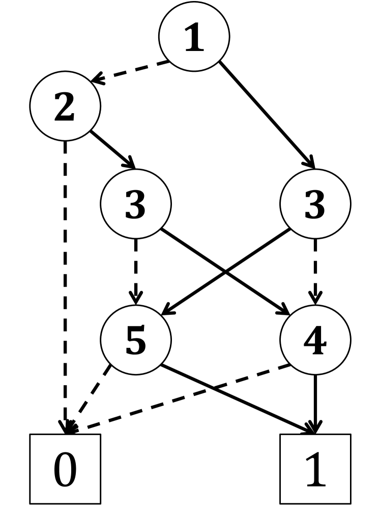
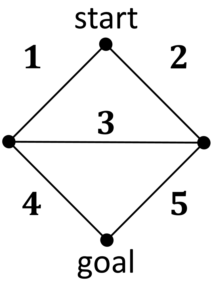
In general, a ZDD is assumed to be ordered and reduced. 𝐆𝒮subscript𝐆𝒮\mathbf{G}_{\mathcal{S}} is said to be ordered if v>ulv<lu𝑣𝑢subscript𝑙𝑣subscript𝑙𝑢v>u\Rightarrow l_{v}<l_{u} holds for all v,uV\{0,1}𝑣𝑢\𝑉01v,u\in V\backslash\{0,1\}. A non-terminal vertex v𝑣v is said to be redundant if cv1=0superscriptsubscriptc𝑣10\mathrm{c}_{v}^{1}=0: its 1-arc directly points to the 0-terminal. A redundant vertex v𝑣v can be removed by replacing all (u,v)A𝑢𝑣𝐴(u,v)\in A with (u,cv0)𝑢superscriptsubscriptc𝑣0(u,\mathrm{c}_{v}^{0}) without loss of the property (4). A non-terminal vertex v𝑣v is said to be sharable if there exists another vertex vsuperscript𝑣v^{\prime} such that lv=lvsubscript𝑙𝑣subscript𝑙superscript𝑣l_{v}=l_{v^{\prime}} and cvb=cvbsuperscriptsubscriptc𝑣𝑏superscriptsubscriptcsuperscript𝑣𝑏\mathrm{c}_{v}^{b}=\mathrm{c}_{v^{\prime}}^{b} (b{0,1})b\in\{0,1\}): v𝑣v and vsuperscript𝑣v^{\prime} have the same label and children. A sharable vertex v𝑣v can be removed by replacing (u,v)A𝑢𝑣𝐴(u,v)\in A with (u,v)𝑢superscript𝑣(u,v^{\prime}). 𝐆𝒮subscript𝐆𝒮\mathbf{G}_{\mathcal{S}} is said to be reduced if no vertex is redundant or sharable. In this paper, we assume that 𝐆𝒮subscript𝐆𝒮\mathbf{G}_{\mathcal{S}} is ordered and reduced. We show an example of a ZDD in Figure 1.
Refer to caption
(a)
Refer to caption
(b)
Figure 1: (a) An example network with an edge set E={1,,5}𝐸15E=\{1,\dots,5\}, and (b) a ZDD that stores all paths from the start to the goal; each non-terminal vertex v𝑣v is labeled lvEsubscript𝑙𝑣𝐸l_{v}\in E, and 00-arcs and 111-arcs are indicated by dashed and solid lines, respectively. Note that we have 𝒮={X(R)Rr,1}={{1,4},{2,5},{1,3,5},{2,3,4}}𝒮conditional-set𝑋𝑅𝑅subscript𝑟11425135234\mathcal{S}=\{X(R)\mid R\in\mathcal{R}_{r,1}\}=\{\{1,4\},\{2,5\},\{1,3,5\},\{2,3,4\}\}.

The ZDDs are known to store various families of sets compactly in many applications. In particular, if a decision set is a set of specific network substructures (e.g, a set of s𝑠s-t𝑡t paths or Steiner trees), the ZDD representing the decision set tends to be small. As we will see later, the time complexity of COMBWM with a ZDD 𝐆𝒮=(V,A)subscript𝐆𝒮𝑉𝐴\mathbf{G}_{\mathcal{S}}=(V,A) is O(d|V|)𝑂𝑑𝑉O(d|V|), and so it runs fast if the ZDD is small. In theory, if 𝒮𝒮\mathcal{S} is a set of specific network substructures, then |V|𝑉|V| is bounded by a value that is exponential in the pathwidth [17]. Thus, even if a network-based decision set is exponentially large in d𝑑d, the time complexity of our algorithm in each round can be polynomial in d𝑑d if the pathwidth of the network is bounded by a small constant.

The frontier-based search [21], which is based on Knuth’s Simpath algorithm [24], has recently received much attention as a fast top-down construction algorithm for ZDDs that represent a family of subnetworks. In practice ZDDs are easily obtained via existing software [16] for various network-based constraints. In this paper, we omit the details of ZDD construction and assume that a decision set 𝒮𝒮\mathcal{S} is represented by a ZDD 𝐆𝒮subscript𝐆𝒮\mathbf{G}_{\mathcal{S}} rather than by the explicit enumeration of the components of 𝒮𝒮\mathcal{S}.

5.2 Sampling from constrained distributions

We here propose an efficient algorithm for sampling from a constrained distribution p(X;𝒘,𝒮)𝑝𝑋𝒘𝒮p(X;\mbox{\boldmath$w$},\mathcal{S}). We first introduce the following forward weight (FW) FvsubscriptF𝑣\mathrm{F}_{v} and backward weight (BW) BvsubscriptB𝑣\mathrm{B}_{v} (vV𝑣𝑉v\in V):

(5) FvsubscriptF𝑣\displaystyle\mathrm{F}_{v} :=Rr,vw(R),assignabsentsubscript𝑅subscript𝑟𝑣𝑤𝑅\displaystyle:=\sum_{R\in\mathcal{R}_{r,v}}w(R), BvsubscriptB𝑣\displaystyle\mathrm{B}_{v} :=Rv,1w(R),assignabsentsubscript𝑅subscript𝑣1𝑤𝑅\displaystyle:=\sum_{R\in\mathcal{R}_{v,1}}w(R),

where w(R)𝑤𝑅w(R) is an abbreviation of w(X(R))=iX(R)wi𝑤𝑋𝑅subscriptproduct𝑖𝑋𝑅subscript𝑤𝑖w(X(R))=\prod_{i\in X(R)}w_{i}. By combining Eq. (1), (4), and (5), we obtain Z(𝒘,𝒮)=Br=F1𝑍𝒘𝒮subscriptB𝑟subscriptF1Z(\mbox{\boldmath$w$},\mathcal{S})=\mathrm{B}_{r}=\mathrm{F}_{1}. B:={B0,,Br}assignBsubscriptB0subscriptB𝑟\mathrm{B}:=\{\mathrm{B}_{0},\dots,\mathrm{B}_{r}\} and F:={F0,,Fr}assignFsubscriptF0subscriptF𝑟\mathrm{F}:=\{\mathrm{F}_{0},\dots,\mathrm{F}_{r}\} can be efficiently computed in a dynamic programming manner on 𝐆𝒮subscript𝐆𝒮\mathbf{G}_{\mathcal{S}} as shown in Algorithm FW(𝐆𝒮,𝒘subscript𝐆𝒮𝒘\mathbf{G}_{\mathcal{S}},\mbox{\boldmath$w$}) and BW(𝐆𝒮,𝒘subscript𝐆𝒮𝒘\mathbf{G}_{\mathcal{S}},\mbox{\boldmath$w$}). Once we obtain BB\mathrm{B}, we can draw a sample from p(X;𝒘,𝒮)𝑝𝑋𝒘𝒮p(X;\mbox{\boldmath$w$},\mathcal{S}) by top-down sampling on 𝐆𝒮subscript𝐆𝒮\mathbf{G}_{\mathcal{S}} without rejections as shown in Algorithm Draw(𝐆𝒮,𝒘,Bsubscript𝐆𝒮𝒘B\mathbf{G}_{\mathcal{S}},\mbox{\boldmath$w$},\mathrm{B}), where Ber(θ)Ber𝜃\mathrm{Ber}\!\left(\theta\right) is the Bernoulli distribution with the parameter θ[0,1]𝜃01\theta\in[0,1]. The space and time complexity when computing FF\mathrm{F} and BB\mathrm{B} is proportional to |V|𝑉|V|. This constrained sampling is based on the same idea as that used in logic-based probabilistic modeling [18, 19].

1:  Algorithm FW(𝐆𝒮,𝒘subscript𝐆𝒮𝒘\mathbf{G}_{\mathcal{S}},\mbox{\boldmath$w$}) 2:  Fr1subscriptF𝑟1\mathrm{F}_{r}\leftarrow 1 3:  Fv0subscriptF𝑣0\mathrm{F}_{v}\leftarrow 0 (vV\{r}for-all𝑣\𝑉𝑟\forall v\in V\backslash\{r\}) 4:  for v=r,,2𝑣𝑟2v=r,\dots,2 do 5:     Fcv0+=Fvlimit-fromsubscriptFsuperscriptsubscriptc𝑣0subscriptF𝑣\mathrm{F}_{\mathrm{c}_{v}^{0}}+\!=\mathrm{F}_{v} 6:     Fcv1+=wlvFvlimit-fromsubscriptFsuperscriptsubscriptc𝑣1subscript𝑤subscript𝑙𝑣subscriptF𝑣\mathrm{F}_{\mathrm{c}_{v}^{1}}+\!=w_{l_{v}}\mathrm{F}_{v} 7:  end for 8:  F:={F0,,Fr}assignFsubscriptF0subscriptF𝑟\mathrm{F}:=\{\mathrm{F}_{0},\dots,\mathrm{F}_{r}\} 9:  return  FF\mathrm{F} 1:  Algorithm BW(𝐆𝒮,𝒘subscript𝐆𝒮𝒘\mathbf{G}_{\mathcal{S}},\mbox{\boldmath$w$}) 2:  B11subscriptB11\mathrm{B}_{1}\leftarrow 1 3:  Bv0subscriptB𝑣0\mathrm{B}_{v}\leftarrow 0 (vV\{1}for-all𝑣\𝑉1\forall v\in V\backslash\{1\}) 4:  for v=2,,r𝑣2𝑟v=2,\dots,r do 5:     BvBcv0+wlvBcv1subscriptB𝑣subscriptBsuperscriptsubscriptc𝑣0subscript𝑤subscript𝑙𝑣subscriptBsuperscriptsubscriptc𝑣1\mathrm{B}_{v}\leftarrow\mathrm{B}_{\mathrm{c}_{v}^{0}}+w_{l_{v}}\mathrm{B}_{\mathrm{c}_{v}^{1}} 6:  end for 7:  B:={B0,,Br}assignBsubscriptB0subscriptB𝑟\mathrm{B}:=\{\mathrm{B}_{0},\dots,\mathrm{B}_{r}\} 8:  return  BB\mathrm{B} 1:  Algorithm Draw(𝐆𝒮,𝒘,Bsubscript𝐆𝒮𝒘B\mathbf{G}_{\mathcal{S}},\mbox{\boldmath$w$},\mathrm{B}) 2:  X{}𝑋X\leftarrow\{\}, vr𝑣𝑟v\leftarrow r 3:  while v>1𝑣1v>1 do 4:     θwlvBcv1/Bv𝜃subscript𝑤subscript𝑙𝑣subscriptBsuperscriptsubscriptc𝑣1subscriptB𝑣\theta\leftarrow w_{l_{v}}\mathrm{B}_{\mathrm{c}_{v}^{1}}/\mathrm{B}_{v} 5:     bBer(θ)similar-to𝑏Ber𝜃b\sim\mathrm{Ber}\!\left(\theta\right) 6:     XX{lv}𝑋𝑋subscript𝑙𝑣X\leftarrow X\cup\{l_{v}\}  if  b=1𝑏1b=1 7:     vcvb𝑣superscriptsubscriptc𝑣𝑏v\leftarrow\mathrm{c}_{v}^{b} 8:  end while 9:  return  X𝑋X

5.3 Computing co-occurrence probabilities

Given a constrained distribution p(X;𝒘,𝒮)𝑝𝑋𝒘𝒮p(X;\mbox{\boldmath$w$},\mathcal{S}), we define Pi,j:=p(iX,jX;𝒘,𝒮)assignsubscriptP𝑖𝑗𝑝formulae-sequence𝑖𝑋𝑗𝑋𝒘𝒮\mathrm{P}_{i,j}:=p(i\in X,j\in X;\mbox{\boldmath$w$},\mathcal{S}) as the co-occurrence probability of i𝑖i and j𝑗j (i,jE𝑖𝑗𝐸i,j\in E). We here propose an efficient algorithm for computing Pi,jsubscriptP𝑖𝑗\mathrm{P}_{i,j} (ij𝑖𝑗i\leq j), which suffices for obtaining Pi,jsubscriptP𝑖𝑗\mathrm{P}_{i,j} for all i,j[d]𝑖𝑗delimited-[]𝑑i,j\in[d] since Pi,j=Pj,isubscriptP𝑖𝑗subscriptP𝑗𝑖\mathrm{P}_{i,j}=\mathrm{P}_{j,i}. Using Eq. (1) and the notion of 𝐆𝒮subscript𝐆𝒮\mathbf{G}_{\mathcal{S}}, Pi,jsubscriptP𝑖𝑗\mathrm{P}_{i,j} can be written as follows:

(6) Pi,jsubscriptP𝑖𝑗\displaystyle\mathrm{P}_{i,j} =Rr,1:i,jX(R)w(R)Z(𝒘,𝒮).absentsubscript:𝑅subscript𝑟1𝑖𝑗𝑋𝑅𝑤𝑅𝑍𝒘𝒮\displaystyle=\sum_{R\in\mathcal{R}_{r,1}:i,j\in X(R)}\frac{w(R)}{Z(\mbox{\boldmath$w$},\mathcal{S})}.

We first consider Pi,isubscriptP𝑖𝑖\mathrm{P}_{i,i} as a special case of Pi,jsubscriptP𝑖𝑗\mathrm{P}_{i,j}. By combining Eq. (5) and (6), we obtain

Pi,isubscriptP𝑖𝑖\displaystyle\mathrm{P}_{i,i} =Rr,1:iX(R)w(R)Z(𝒘,𝒮)=vV:lv=iRr,vR′′cv1,1w(R{i}R′′)Br=vV:lv=iFvwiBcv1Br.absentsubscript:𝑅subscript𝑟1𝑖𝑋𝑅𝑤𝑅𝑍𝒘𝒮subscript:𝑣𝑉subscript𝑙𝑣𝑖subscriptsuperscript𝑅subscript𝑟𝑣superscript𝑅′′subscriptsuperscriptsubscriptc𝑣11𝑤superscript𝑅𝑖superscript𝑅′′subscriptB𝑟subscript:𝑣𝑉subscript𝑙𝑣𝑖subscriptF𝑣subscript𝑤𝑖subscriptBsuperscriptsubscriptc𝑣1subscriptB𝑟\displaystyle=\sum_{R\in\mathcal{R}_{r,1}:i\in X(R)}\frac{w(R)}{Z(\mbox{\boldmath$w$},\mathcal{S})}=\sum_{v\in V:l_{v}=i}\sum_{\begin{subarray}{c}R^{\prime}\in\mathcal{R}_{r,v}\\ R^{\prime\prime}\in\mathcal{R}_{\mathrm{c}_{v}^{1},1}\end{subarray}}\frac{w(R^{\prime}\cup\{i\}\cup R^{\prime\prime})}{\mathrm{B}_{r}}=\sum_{v\in V:l_{v}=i}\frac{\mathrm{F}_{v}w_{i}\mathrm{B}_{\mathrm{c}_{v}^{1}}}{\mathrm{B}_{r}}.

Next, to compute Pi,jsubscriptP𝑖𝑗\mathrm{P}_{i,j} (i<j)𝑖𝑗(i<j), we rewrite the right hand side of Eq. (6) using the backward weighted co-occurrence (BWC) Cv,jsubscriptC𝑣𝑗\mathrm{C}_{v,j} (jlv𝑗subscript𝑙𝑣j\geq l_{v}) as follows:

Pi,j=vV:lv=iFvwiCcv1,jBr,subscriptP𝑖𝑗subscript:𝑣𝑉subscript𝑙𝑣𝑖subscriptF𝑣subscript𝑤𝑖subscriptCsuperscriptsubscriptc𝑣1𝑗subscriptB𝑟\displaystyle\mathrm{P}_{i,j}=\sum_{v\in V:l_{v}=i}\frac{\mathrm{F}_{v}w_{i}\mathrm{C}_{\mathrm{c}_{v}^{1},j}}{\mathrm{B}_{r}}, Cv,jsubscriptC𝑣𝑗\displaystyle\mathrm{C}_{v,j} :=Rv,1:jX(R)w(R).assignabsentsubscript:𝑅subscript𝑣1𝑗𝑋𝑅𝑤𝑅\displaystyle:=\sum_{R\in\mathcal{R}_{v,1}:j\in X(R)}w(R).

Because Cv,jsubscriptC𝑣𝑗\mathrm{C}_{v,j} is a variant of BvsubscriptB𝑣\mathrm{B}_{v}, C:={Cv,jvV,jlv}assignCconditional-setsubscriptC𝑣𝑗formulae-sequence𝑣𝑉𝑗subscript𝑙𝑣\mathrm{C}:=\{\mathrm{C}_{v,j}\mid v\in V,j\geq l_{v}\} can be computed in a similar manner to BB\mathrm{B} as shown in Algorithm BWC(𝐆𝒮,𝒘,Bsubscript𝐆𝒮𝒘B\mathbf{G}_{\mathcal{S}},\mbox{\boldmath$w$},\mathrm{B}). To conclude, Pi,jsubscriptP𝑖𝑗\mathrm{P}_{i,j} can be computed by Algorithm CPM(𝐆𝒮,𝒘,F,B,Csubscript𝐆𝒮𝒘FBC\mathbf{G}_{\mathcal{S}},\mbox{\boldmath$w$},\mathrm{F},\mathrm{B},\mathrm{C}). The total space and time complexity of computing P:={Pi,jij}assignPconditional-setsubscriptP𝑖𝑗𝑖𝑗\mathrm{P}:=\{\mathrm{P}_{i,j}\mid i\leq j\} is O(d|V|)𝑂𝑑𝑉O(d|V|).

1:  Algorithm BWC(𝐆𝒮,𝒘,Bsubscript𝐆𝒮𝒘B\mathbf{G}_{\mathcal{S}},\mbox{\boldmath$w$},\mathrm{B}) 2:  Cv,j0subscriptC𝑣𝑗0\mathrm{C}_{v,j}\leftarrow 0 (vVfor-all𝑣𝑉\forall v\in V, jEfor-all𝑗𝐸\forall j\in E) 3:  for v=2,,r𝑣2𝑟v=2,\dots,r do 4:     Cv,lvwlvBcv1subscriptC𝑣subscript𝑙𝑣subscript𝑤subscript𝑙𝑣subscriptBsuperscriptsubscriptc𝑣1\mathrm{C}_{v,l_{v}}\leftarrow w_{l_{v}}\mathrm{B}_{\mathrm{c}_{v}^{1}} 5:     for j=lv+1,,d𝑗subscript𝑙𝑣1𝑑j=l_{v}+1,\dots,d do 6:        Cv,jCcv0,j+wlvCcv1,jsubscriptC𝑣𝑗subscriptCsuperscriptsubscriptc𝑣0𝑗subscript𝑤subscript𝑙𝑣subscriptCsuperscriptsubscriptc𝑣1𝑗\mathrm{C}_{v,j}\leftarrow\mathrm{C}_{\mathrm{c}_{v}^{0},j}+w_{l_{v}}\mathrm{C}_{\mathrm{c}_{v}^{1},j} 7:     end for 8:  end for 9:  C:={Cv,jvV,jlv}assignCconditional-setsubscriptC𝑣𝑗formulae-sequence𝑣𝑉𝑗subscript𝑙𝑣\mathrm{C}:=\{\mathrm{C}_{v,j}\mid v\in V,j\geq l_{v}\} 10:  return  CC\mathrm{C} 1:  Algorithm CPM(𝐆𝒮,𝒘,B,F,Csubscript𝐆𝒮𝒘BFC\mathbf{G}_{\mathcal{S}},\mbox{\boldmath$w$},\mathrm{B},\mathrm{F},\mathrm{C}) 2:  Pi,j0subscriptP𝑖𝑗0\mathrm{P}_{i,j}\leftarrow 0 (i,jEfor-all𝑖𝑗𝐸\forall i,j\in E) 3:  for v=2,,r𝑣2𝑟v=2,\dots,r do 4:     ilv𝑖subscript𝑙𝑣i\leftarrow l_{v} 5:     Pi,i+=FvwiBcv1/Brlimit-fromsubscriptP𝑖𝑖subscriptF𝑣subscript𝑤𝑖subscriptBsuperscriptsubscriptc𝑣1subscriptB𝑟\mathrm{P}_{i,i}+\!=\mathrm{F}_{v}w_{i}\mathrm{B}_{\mathrm{c}_{v}^{1}}/\mathrm{B}_{r} 6:     for j=i+1,,d𝑗𝑖1𝑑j=i+1,\dots,d do 7:        Pi,j+=FvwiCcv1,j/Brlimit-fromsubscriptP𝑖𝑗subscriptF𝑣subscript𝑤𝑖subscriptCsuperscriptsubscriptc𝑣1𝑗subscriptB𝑟\mathrm{P}_{i,j}+\!=\mathrm{F}_{v}w_{i}\mathrm{C}_{\mathrm{c}_{v}^{1},j}/\mathrm{B}_{r} 8:     end for 9:  end for 10:  P:={Pi,ji,j[d],ij}assignPconditional-setsubscriptP𝑖𝑗formulae-sequence𝑖𝑗delimited-[]𝑑𝑖𝑗\mathrm{P}:=\{\mathrm{P}_{i,j}\mid i,j\in[d],i\leq j\} 11:  return  PP\mathrm{P}

6 Experiments

We applied our COMBWM with ZDDs to three network-based CMAB problems: the OSP, DST, and CG. In the OSP and DST, we used artificial networks to observe the scalability of our algorithm. In the CG, we used two real-world networks to show the practical utility of our algorithm. We implemented our algorithm in the C programming language and used Graphillion [16] to obtain the ZDDs. We note that constructing ZDDs with the software is not a drawback; in all of the following instances a ZDD was obtained within at most several seconds.

6.1 OSP and DST on artificial networks

Experimental Setting: We applied our COMBWM with ZDDs to the OSP and DST instances on artificial networks, which are undirected grid networks with 3×m3𝑚3\times m nodes (m=3,,10𝑚310m=3,\dots,10). In both problems, an arm corresponds to an edge of the given network. In the OSP, a decision set 𝒮𝒮\mathcal{S} is a set of all s𝑠s-t𝑡t paths from the starting node s𝑠s to the goal node t𝑡t that are placed on diagonal corners of the given grid. In the DST, 𝒮𝒮\mathcal{S} is a set of all Steiner trees that contains the four corners of the grid. The aim of the player is to minimize the cumulative cost of the selected subnetworks over some time horizon. In this experiment, we define the loss vector tsubscriptbold-ℓ𝑡\mbox{\boldmath$\ell$}_{t} as follows: We first uniformly sample 𝝁0subscript𝝁0\mbox{\boldmath$\mu$}_{0} from [0,1]dsuperscript01𝑑[0,1]^{d}. In the t𝑡t-th round, we set 𝝁t=𝝁t1subscript𝝁𝑡subscript𝝁𝑡1\mbox{\boldmath$\mu$}_{t}=\mbox{\boldmath$\mu$}_{t-1} with probability 0.90.90.9 or draw a new 𝝁tsubscript𝝁𝑡\mbox{\boldmath$\mu$}_{t} uniformly from [0,1]dsuperscript01𝑑[0,1]^{d} with probability 0.10.10.1. Then, for each iE𝑖𝐸i\in E, we draw hiBer(μt,i)similar-tosubscript𝑖Bersubscript𝜇𝑡𝑖h_{i}\sim\mathrm{Ber}\!\left(\mu_{t,i}\right) and set t,i=1/dsubscript𝑡𝑖1𝑑\ell_{{t},{i}}=1/d if ht=1subscript𝑡1h_{t}=1 otherwise 1/d1𝑑-1/d. This setting is a stochastic CMAB with distributions Ber(μt,i)Bersubscript𝜇𝑡𝑖\mathrm{Ber}\!\left(\mu_{t,i}\right) in the short run, but the adversary secretly reset 𝝁tsubscript𝝁𝑡\mbox{\boldmath$\mu$}_{t} with probability 0.10.10.1 in each round to foil the player.

Compression Power: We first assess the compression power of ZDDs constructed for the decision sets of the OSP and DST instances. Table 1 shows the sizes of decision sets 𝒮𝒮\mathcal{S} and those of the corresponding ZDDs 𝐆𝒮subscript𝐆𝒮\mathbf{G}_{\mathcal{S}}. In both problems, the ZDD size, |V|𝑉|V|, grows much more slowly than |𝒮|𝒮|\mathcal{S}|. In particular, with the DST on the 3×103103\times 10 grid, we see that |V|𝑉|V| is five orders of magnitude smaller than |𝒮|𝒮|\mathcal{S}|. In such cases, our COMBWM, which only deals with a ZDD 𝐆𝒮subscript𝐆𝒮\mathbf{G}_{\mathcal{S}}, is much more scalable than the naive method that directly deals with 𝒮𝒮\mathcal{S}.

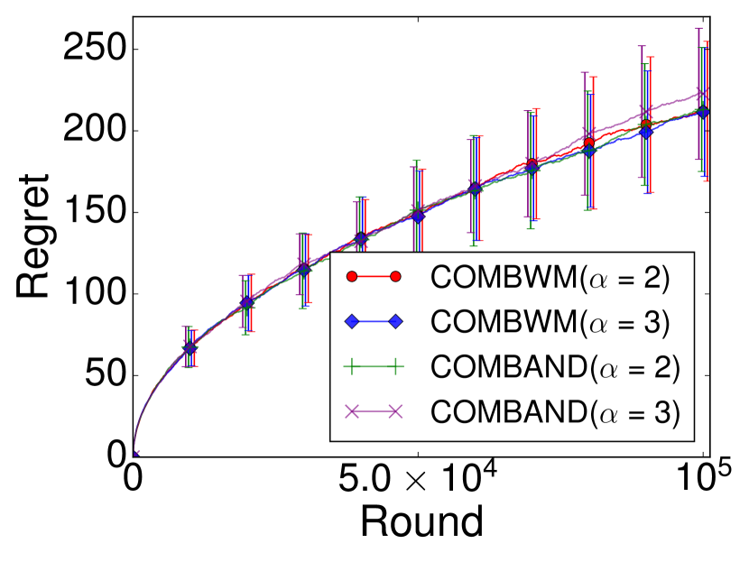
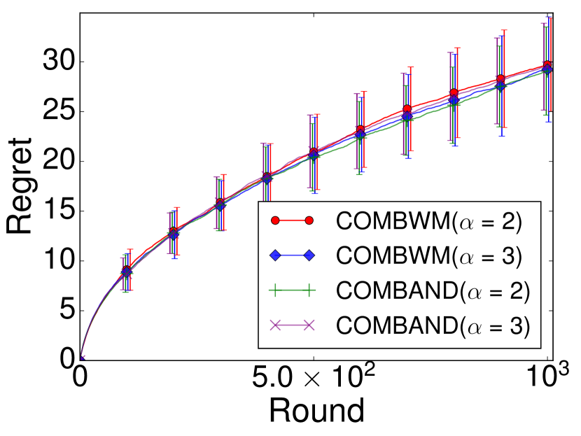
Empirical Regret: We next show that the empirical regrets of our COMBWM and COMBAND actually grow sublinearly, where COMBAND is also performed on ZDDs. We applied these algorithms to the OSP and DST on a 3×103103\times 10 grid and computed their empirical regrets over a time horizon. Figures 2 (a) and (b) summarize their regrets for the OSP and DST, respectively. We see that all of the algorithms achieved more or less the same sublinear regrets. It was confirmed that all of the regret values were lower than those of the theoretical bounds stated in Theorem 1 and Theorem 2; the precise values of the bounds are provided in the supplementary materials.

Table 1: The sizes of decision sets 𝒮𝒮\mathcal{S} and the corresponding ZDDs 𝐆𝒮subscript𝐆𝒮\mathbf{G}_{\mathcal{S}} for the OSP and DST (numbers with more than six digits are rounded to three significant digits).
m𝑚m 3 4 5 6 7 8 9 10
OSP |𝒮|𝒮|\mathcal{S}| 12 38 125 414 1,369 4,522 14,934 49,322
|V|𝑉|V| 31 76 183 451 1,039 2,287 4,991 11,071
DST |𝒮|𝒮|\mathcal{S}| 266 4,285 69,814 1.14×10⁶absentsuperscript106\times 10^{6} 1.86×10⁷absentsuperscript107\times 10^{7} 3.04×10⁸absentsuperscript108\times 10^{8} 4.97×10⁹absentsuperscript109\times 10^{9} 8.12×10¹⁰absentsuperscript1010\times 10^{10}
|V|𝑉|V| 80 304 1,147 4,616 18,032 67,484 238,364 933,394
Refer to caption
(a) OSP on the 3×103103\times 10 grid
Refer to caption
(b) DST on the 3×103103\times 10 grid
Refer to caption
(c) CG on MCI
Refer to caption
(d) CG on ATT
Refer to caption
(e) MCI
Refer to caption
(f) ATT
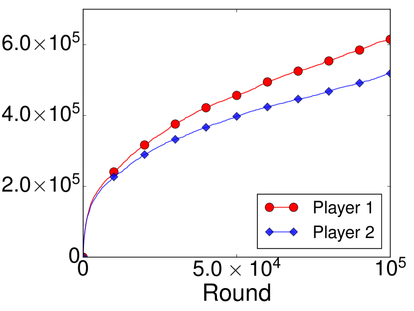
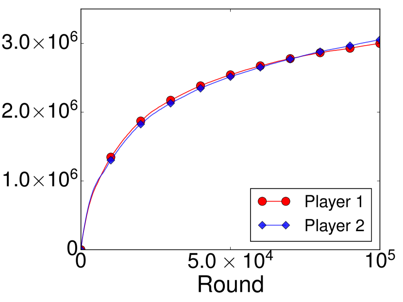
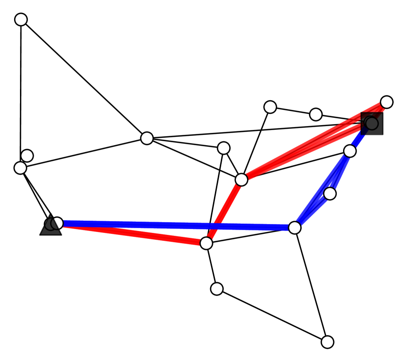
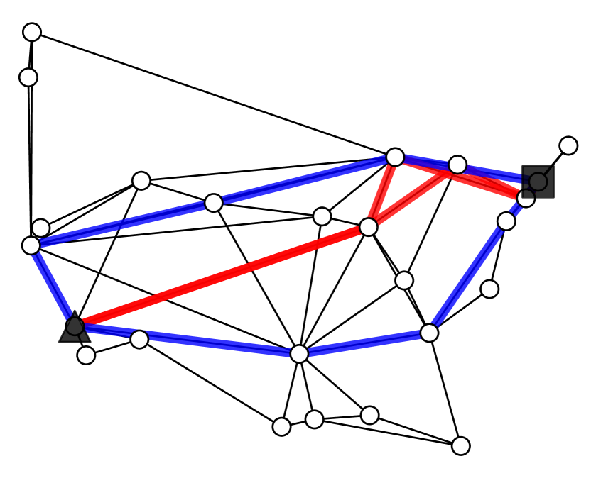
Figure 2: (a) and (b) show the regret values for the OSP and DST, respectively. The regret values are averaged over 100 trials and the error bars indicate the standard deviations. (c) and (d) show the regret values of each player for the CG on the MCI and ATT, respectively. (e) and (f) are the topologies of the two networks; the triangles are the starting nodes and the squares are the goal nodes. The red (blue) paths indicate the top two paths most frequently chosen by player 1 (2).

6.2 CG on real-world networks

Experimental Setting: We applied our COMBWM with ZDDs to the CG, which is a multi-player version of the OSP, on two real-world networks. The CG is described as follows: Given m𝑚m players and an undirected network with a starting node s𝑠s and a goal node t𝑡t, the players concurrently send a message from s𝑠s to t𝑡t. The aim of each player is to minimize the cumulative time needed to send T𝑇T messages. In this problem an arm corresponds to an edge of a given network, and a super arm is an s𝑠s-t𝑡t path. The loss value of an arm is the transmission time required when using the edge, and the cost of a super arm is the total transmission time needed to send a message along the selected s𝑠s-t𝑡t path. In the experiments, we assume that the loss of each edge increases with the number of players who use the same edge at the same time; therefore, a player regards the other players as adversaries. We use Xtk𝒮superscriptsubscript𝑋𝑡𝑘𝒮X_{t}^{k}\in\mathcal{S} (k[m]𝑘delimited-[]𝑚k\in[m]) to denote the k𝑘k-th player’s choice in the t𝑡t-th round and use Xt,ik{0,1}superscriptsubscript𝑋𝑡𝑖𝑘01X_{t,i}^{k}\in\{0,1\} to denote the i𝑖i-th element of 𝟏Xtksubscript1superscriptsubscript𝑋𝑡𝑘\mbox{\boldmath$1$}_{X_{t}^{k}}. We also use t,iksuperscriptsubscript𝑡𝑖𝑘\ell_{t,i}^{k} to denote the transmission time that the k𝑘k-th player consumes when sending a message using the i𝑖i-th edge at the t𝑡t-th round. We here define t,ik:=βiκNt,ikassignsuperscriptsubscript𝑡𝑖𝑘subscript𝛽𝑖superscript𝜅superscriptsubscript𝑁𝑡𝑖𝑘\ell_{{t},{i}}^{k}:=\beta_{i}\kappa^{N_{t,i}^{-k}}, where βisubscript𝛽𝑖\beta_{i}\in\mathbb{R} is the length of the edge, κ𝜅\kappa is an overhead constant, and Nt,ik:=kkXt,ikassignsuperscriptsubscript𝑁𝑡𝑖𝑘subscriptsuperscript𝑘𝑘superscriptsubscript𝑋𝑡𝑖superscript𝑘N_{t,i}^{-k}:=\sum_{k^{\prime}\not=k}X_{t,i}^{k^{\prime}} is the number of adversaries who also choose the i𝑖i-th edge at the t𝑡t-th round. Namely, we assume that the transmission time of each edge increases exponentially with the number of players using the same edge at the same time. Consequently, to reduce the total transmission time, the players should adaptively avoid contending with each other. Note that this setting violates the assumption |ct|<1subscript𝑐𝑡1|c_{t}|<1; however, in practice, this violation barely matters. In the experiments, we set m=2𝑚2m=2 and κ=10𝜅10\kappa=10.

We use two real-world communication networks in the Internet topology zoo [23]: the InternetMCI network (MCI) and the ATT North America network (ATT). Figure 2 (e) and (f) illustrate the topologies of the MCI and ATT, respectively. Both networks correspond to the U.S. map and we choose Los Angeles as the starting point s𝑠s and New York as the goal t𝑡t. The statistics for each network are shown in Table 2.

Table 2: Statistics for two real-world communication networks.
Network # nodes # edges # s𝑠s-t𝑡t paths |𝒮|𝒮|\mathcal{S}| ZDD size |V|𝑉|V|
MCI 19 33 1,444 756
ATT 25 56 213,971 37,776

Experimental Results: Figures 2 (c) and (d) show the regret values of each player for the MCI and ATT, respectively. The figure shows that each player attained sublinear regrets. Figures 2 (e) and (f) show the top two most frequently selected paths for each player. We see that each player successfully avoided congestion. In the full information setting where the players can observe the costs of all s𝑠s-t𝑡t paths after choosing the current path, it is known that the Hedge algorithm [13] can achieve the Nash equilibria [22] on the CG. In this experiment, even though we employed the bandit setting where each player can only observe the cost of the selected path, the players successfully found almost optimal strategies on both networks. To conclude, the experimental results suggest that our algorithm is useful for adaptive routing problems on real-world networks.

7 Conclusion

We proposed COMBWM with ZDDs, which is a practical and theoretically guaranteed algorithm for the adversarial CMAB. We also showed that our algorithm is effective for network-based adversarial CMAB instances, which include various important problems such as the OSP, DST, and CG. The efficiency of our algorithm is thanks to the compression of the decision sets via ZDDs, and its time and space complexities are linear in the size of ZDDs; more precisely, they are O(d|V|)𝑂𝑑𝑉O(d|V|). We showed experimentally that the ZDDs for the OSP, DST, and CG are much smaller in size than original decision sets. Our algorithm is also theoretically guaranteed to achieve either O(T2/3)𝑂superscript𝑇23O(T^{2/3}) regret with high probability or O(T)𝑂𝑇O(\sqrt{T}) expected regret as an any-time guarantee; we experimentally confirmed that our algorithm attained sublinear regrets. The results on CG showed that our algorithm is useful for adaptive routing problems on real-world networks.

References

  • [1] N. Ailon, K. Hatano, and E. Takimoto. Bandit online optimization over the permutahedron. In International Conference on Algorithmic Learning Theory, pages 215–229. Springer, 2014.
  • [2] R. Arora, O. Dekel, and A. Tewari. Online bandit learning against an adaptive adversary: from regret to policy regret. arXiv preprint arXiv:1206.6400, 2012.
  • [3] J.-Y. Audibert, S. Bubeck, and G. Lugosi. Regret in online combinatorial optimization. Math. Oper. Res., 39(1):31–45, February 2014.
  • [4] B. Awerbuch and R. D. Kleinberg. Adaptive routing with end-to-end feedback: Distributed learning and geometric approaches. In 36th Annual ACM Symposium on Theory of Computing, pages 45–53. ACM, 2004.
  • [5] P. L. Bartlett, V. Dani, T. Hayes, S. Kakade, A. Rakhlin, and A. Tewari. High-probability regret bounds for bandit online linear optimization. In 21st Annual Conference on Learning Theory, pages 335–342. Omnipress, 2008.
  • [6] D. Bergman, A. A. Cire, W.-J. van Hoeve, and J. Hooker. Decision Diagrams for Optimization. Springer, first edition, 2016.
  • [7] G. Braun and S. Pokutta. An efficient high-probability algorithm for linear bandits. arXiv preprint arXiv:1610.02072, 2016.
  • [8] S. Bubeck, N. Cesa-Bianchi, and S. M. Kakade. Towards minimax policies for online linear optimization with bandit feedback. In Conference on Learning Theory, pages 1–14, 2012.
  • [9] N. Cesa-Bianchi and G. Lugosi. Combinatorial bandits. J. Comput. Syst. Sci., 78(5):1404 – 1422, 2012.
  • [10] R. Combes, M. Sadegh Talebi, A. Proutiere, and M. Lelarge. Combinatorial bandits revisited. In Advances in Neural Information Processing Systems, pages 2116–2124, 2015.
  • [11] O. Coudert. Solving graph optimization problems with ZBDDs. In 1997 European Conference on Design and Test, page 224. IEEE Computer Society, 1997.
  • [12] X. Fan, I. Grama, and Q. Liu. Hoeffding’s inequality for supermartingales. Stoch. Proc. Appl., 122(10):3545–3559, 2012.
  • [13] Y. Freund and R. E. Schapire. Adaptive game playing using multiplicative weights. Games Econom. Behav., 29(1):79 – 103, 1999.
  • [14] A. György, T. Linder, G. Lugosi, and G. Ottucsák. The on-line shortest path problem under partial monitoring. J. Mach. Learn. Res., 8(Oct):2369–2403, 2007.
  • [15] M. Imase and B. M. Waxman. Dynamic Steiner tree problem. SIAM J. Discrete. Math., 4(3):369–384, 1991.
  • [16] T. Inoue, H. Iwashita, J. Kawahara, and S. Minato. Graphillion: software library for very large sets of labeled graphs. Int. J. Software Tool. Tech. Tran., 18(1):57–66, 2016.
  • [17] Y. Inoue and S. Minato. Acceleration of ZDD construction for subgraph enumeration via path-width optimization. Technical report, TCS-TR-A-16-80, Hokkaido University, 2016.
  • [18] M. Ishihata, Y. Kameya, T. Sato, and S. Minato. Propositionalizing the EM algorithm by BDDs. In 18th International Conference on Inductive Logic Programming, pages 44–49, 2008.
  • [19] M. Ishihata and T. Sato. Bayesian inference for statistical abduction using Markov chain Monte Carlo. In 3rd Asian Conference on Machine Learning, pages 81–96, 2011.
  • [20] S. Kale, L. Reyzin, and R. E. Schapire. Non-stochastic bandit slate problems. In Advances in Neural Information Processing Systems, pages 1054–1062, 2010.
  • [21] J. Kawahara, T. Inoue, H. Iwashita, and S. Minato. Frontier-based search for enumerating all constrained subgraphs with compressed representation. Technical report, TCS-TR-A-14-76, Hokkaido University, 2014.
  • [22] R. Kleinberg, G. Piliouras, and E. Tardos. Multiplicative updates outperform generic no-regret learning in congestion games: Extended abstract. In 41st Annual ACM Symposium on Theory of Computing, pages 533–542. ACM, 2009.
  • [23] S. Knight, H. X. Nguyen, N. Falkner, R. Bowden, and M. Roughan. The Internet topology zoo. IEEE J. Sel. Area. Comm., 29(9):1765–1775, 2011.
  • [24] D. E. Knuth. The Art of Computer Programming: Combinatorial Algorithms, Part 1, volume 4A. Addison-Wesley Professional, 1st edition, 2011.
  • [25] V. Kuleshov and D. Precup. Algorithms for multi-armed bandit problems. arXiv preprint arXiv:1402.6028, 2014.
  • [26] L. Li, W. Chu, J. Langford, and R. E. Schapire. A contextual-bandit approach to personalized news article recommendation. In 19th international conference on World wide web, pages 661–670. ACM, 2010.
  • [27] S. Minato. Zero-suppressed BDDs for set manipulation in combinatorial problems. In 30th International Design Automation Conference, pages 272–277. ACM, 1993.
  • [28] D. R. Morrison, E. C. Sewell, and S. H. Jacobson. Solving the pricing problem in a branch-and-price algorithm for graph coloring using zero-suppressed binary decision diagrams. INFORMS J. Comput., 28(1):67–82, 2016.
  • [29] H. Robbins. Some aspects of the sequential design of experiments. In Herbert Robbins Selected Papers, pages 169–177. Springer, 1985.
  • [30] R. W. Rosenthal. A class of games possessing pure-strategy Nash equilibria. Internat. J. Game Theory, 2(1):65–67, 1973.
  • [31] T. Uchiya, A. Nakamura, and M. Kudo. Algorithms for adversarial bandit problems with multiple plays. In International Conference on Algorithmic Learning Theory, pages 375–389. Springer, 2010.

Supplementary material

In what follows we prove Theorem 1 and Theorem 2. Section S1 presents two concentration inequalities that are important in the proofs. In Section S2 we provide some preliminaries for the proofs. Section S3 and Section S4 provide the proofs of Theorem 1 and Theorem 2, respectively.

S1 Concentration inequalities

The following concentration inequalities play crucial roles in the subsequent discussion.

Theorem 3 (Azuma-Hoeffding inequality).

If a martingale difference sequence {Zt}t=1Tsuperscriptsubscriptsubscript𝑍𝑡𝑡1𝑇\{Z_{t}\}_{t=1}^{T} satisfies atZtbtsubscript𝑎𝑡subscript𝑍𝑡subscript𝑏𝑡a_{t}\leq Z_{t}\leq b_{t} almost surely with some constants at,btsubscript𝑎𝑡subscript𝑏𝑡a_{t},b_{t} for t=1,,T𝑡1𝑇t=1,\dots,T, then the following inequality holds with probability at least 1δ1𝛿1-\delta:

t=1TZtln(1/δ)2t=1T(btat)2.superscriptsubscript𝑡1𝑇subscript𝑍𝑡1𝛿2superscriptsubscript𝑡1𝑇superscriptsubscript𝑏𝑡subscript𝑎𝑡2\sum_{t=1}^{T}Z_{t}\leq\sqrt{\frac{\ln(1/\delta)}{2}\sum_{t=1}^{T}(b_{t}-a_{t})^{2}}.
Theorem 4 (Bennett’s inequality [12]).

If a supermartingale difference sequence {Zt}t=1Tsuperscriptsubscriptsubscript𝑍𝑡𝑡1𝑇\{Z_{t}\}_{t=1}^{T} with respect to a filtration {t}t=0T1superscriptsubscriptsubscript𝑡𝑡0𝑇1\{\mathcal{F}_{t}\}_{t=0}^{T-1} satisfies Ztbsubscript𝑍𝑡𝑏Z_{t}\leq b with some constant b>0𝑏0b>0 for t=1,,T𝑡1𝑇t=1,\dots,T, then, for any v0𝑣0v\geq 0, we have the following with probability at least 1δ1𝛿1-\delta:

t=1TVar[Ztt1]vort=1TZtb3ln1δ+2vln1δ.formulae-sequencesuperscriptsubscript𝑡1𝑇Vardelimited-[]conditionalsubscript𝑍𝑡subscript𝑡1𝑣orsuperscriptsubscript𝑡1𝑇subscript𝑍𝑡𝑏31𝛿2𝑣1𝛿\sum_{t=1}^{T}\text{Var}[{Z_{t}\mid\mathcal{F}_{t-1}}]\geq v\quad\text{or}\quad\sum_{t=1}^{T}Z_{t}\leq\frac{b}{3}\ln\frac{1}{\delta}+\sqrt{2v\ln\frac{1}{\delta}}.

S2 Preliminaries for the proofs

Algorithm 2 COMBWM(α,𝒮)𝛼𝒮(\alpha,\mathcal{S})
1:  w~1,i1subscript~𝑤1𝑖1\widetilde{w}_{{1},{i}}\leftarrow 1 and w1,i1subscript𝑤1𝑖1w_{{1},{i}}\leftarrow 1 (iE𝑖𝐸i\in E)
2:  for t=1,,T𝑡1𝑇t=1,\dots,T do
3:     γtt1/α2subscript𝛾𝑡superscript𝑡1𝛼2\gamma_{t}\leftarrow\frac{t^{-1/\alpha}}{2}, ηtλt1/α2L2subscript𝜂𝑡𝜆superscript𝑡1𝛼2superscript𝐿2\eta_{t}\leftarrow\frac{\lambda t^{-1/\alpha}}{2L^{2}}, ηt+1λ(t+1)1/α2L2subscript𝜂𝑡1𝜆superscript𝑡11𝛼2superscript𝐿2\eta_{t+1}\leftarrow\frac{\lambda(t+1)^{-1/\alpha}}{2L^{2}}
4:     Xtptsimilar-tosubscript𝑋𝑡subscript𝑝𝑡X_{t}\sim p_{t}
5:     ctt𝟏Xtsubscript𝑐𝑡superscriptsubscriptbold-ℓ𝑡topsubscript1subscript𝑋𝑡c_{t}\leftarrow\mbox{\boldmath$\ell$}_{t}^{\top}\mbox{\boldmath$1$}_{{X_{t}}} (tsubscriptbold-ℓ𝑡\mbox{\boldmath$\ell$}_{t} is unobservable)
6:     Pt(1γt)Qt+γtUsubscript𝑃𝑡1subscript𝛾𝑡subscript𝑄𝑡subscript𝛾𝑡𝑈P_{t}\leftarrow(1-\gamma_{t})Q_{t}+\gamma_{t}U
7:     ^tctPt+𝟏Xtsubscriptbold-^bold-ℓ𝑡subscript𝑐𝑡superscriptsubscript𝑃𝑡subscript1subscript𝑋𝑡\mbox{{\boldmath$\hat{\ell}$}}_{t}\leftarrow c_{t}P_{t}^{+}\mbox{\boldmath$1$}_{{X_{t}}}
8:     wt+1,iw~t,iexp(ηt^t,i)subscript𝑤𝑡1𝑖subscript~𝑤𝑡𝑖subscript𝜂𝑡subscript^𝑡𝑖w_{{t+1},{i}}\leftarrow\widetilde{w}_{{t},{i}}\exp\big{(}-\eta_{t}{\hat{\ell}}_{{t},{i}}\big{)} (iE)𝑖𝐸(i\in E)
9:     w~t+1,iwt+1,iηt+1/ηtsubscript~𝑤𝑡1𝑖superscriptsubscript𝑤𝑡1𝑖subscript𝜂𝑡1subscript𝜂𝑡\widetilde{w}_{{t+1},{i}}\leftarrow w_{{t+1},{i}}^{{\eta_{t+1}}/{\eta_{t}}} (iE)𝑖𝐸(i\in E)
10:  end for
11:  return  {Xtt[T]}conditional-setsubscript𝑋𝑡𝑡delimited-[]𝑇\{X_{t}\mid t\in[T]\}

We here rewrite Algorithm 1 equivalently as in Algorithm 2, which will be helpful in terms of understanding the subsequent discussion. In what follows, we let K:=|𝒮|assign𝐾𝒮K:=|\mathcal{S}| and μ:=1/Kassign𝜇1𝐾\mu:=1/K. We also define 𝔼t[]:=𝔼[X1:t1,1:t]\mathbb{E}_{t}[\cdot]:=\mathbb{E}[\cdot\mid{X_{{1:t-1}}},{{\text{\boldmath{$\ell$}}}_{{1:t}}}] as the conditional expectation in the t𝑡t-th round given all the history of rounds 1,,t11𝑡11,\dots,t-1 and the loss vector in round t𝑡t. Similarly, we define the conditional variance in round t𝑡t as Vart[]:=Var[X1:t1,1:t]\text{Var}_{t}[{\cdot}]:=\text{Var}[{\cdot\mid{X_{{1:t-1}}},{{\text{\boldmath{$\ell$}}}_{{1:t}}}}]. For any vector 𝒙=(x1,,xn)n𝒙superscriptsubscript𝑥1subscript𝑥𝑛topsuperscript𝑛\mbox{\boldmath$x$}=(x_{1},\dots,x_{n})^{\top}\in\mathbb{R}^{n} and p>0𝑝0p>0, we define the p𝑝p-norm of 𝒙𝒙x as 𝒙p:=(i=1n|xi|p)1/passignsubscriptnorm𝒙𝑝superscriptsuperscriptsubscript𝑖1𝑛superscriptsubscript𝑥𝑖𝑝1𝑝\|\mbox{\boldmath$x$}\|_{p}:=(\sum_{i=1}^{n}|x_{i}|^{p})^{1/p}, and we often use 𝒙norm𝒙\|\mbox{\boldmath$x$}\| to express 𝒙2subscriptnorm𝒙2\|\mbox{\boldmath$x$}\|_{2}. For any matrix Pn×n𝑃superscript𝑛𝑛P\in\mathbb{R}^{n\times n}, we denote its i,j𝑖𝑗i,j entry as P(i,j)𝑃𝑖𝑗P(i,j). We define the trace of P𝑃P as Tr(P):=i=1nP(i,i)assignTr𝑃superscriptsubscript𝑖1𝑛𝑃𝑖𝑖\text{Tr}(P):=\sum_{i=1}^{n}P(i,i) and denote the spectral norm of P𝑃P as Pnorm𝑃\|P\|, i.e., Pnorm𝑃\|P\| is the largest singular value of P𝑃P. For any symmetric matrices P,Qn×n𝑃𝑄superscript𝑛𝑛P,Q\in\mathbb{R}^{n\times n}, we use PQsucceeds-or-equals𝑃𝑄P\succeq Q to express the fact that the smallest eigenvalue of PQ𝑃𝑄P-Q is non-negative.

For all t[T]𝑡delimited-[]𝑇t\in[T], we define distributions u𝑢u and qtsubscript𝑞𝑡q_{t} over 𝒮𝒮\mathcal{S}, and d×d𝑑𝑑d\times d matrices U𝑈U and Qtsubscript𝑄𝑡Q_{t} as follows:

u(X):=p(X;𝟏E,𝒮)=μ,assign𝑢𝑋𝑝𝑋subscript1𝐸𝒮𝜇\displaystyle u(X):=p(X;\mbox{\boldmath$1$}_{E},\mathcal{S})=\mu, qt(X):=p(X;𝒘~t,𝒮)=w~t(X)X𝒮w~t(X),assignsubscript𝑞𝑡𝑋𝑝𝑋subscriptbold-~𝒘𝑡𝒮subscript~𝑤𝑡𝑋subscriptsuperscript𝑋𝒮subscript~𝑤𝑡superscript𝑋\displaystyle q_{t}(X):=p(X;\mbox{{\boldmath$\widetilde{w}$}}_{t},\mathcal{S})=\frac{{\widetilde{w}}_{t}(X)}{\sum_{X^{\prime}\in\mathcal{S}}{\widetilde{w}}_{t}(X^{\prime})},
U:=𝔼Xu[𝟏X𝟏X]=X𝒮μ𝟏X𝟏X,assign𝑈subscript𝔼similar-to𝑋𝑢delimited-[]subscript1𝑋superscriptsubscript1𝑋topsubscript𝑋𝒮𝜇subscript1𝑋superscriptsubscript1𝑋top\displaystyle U:=\mathbb{E}_{X\sim u}[\mbox{\boldmath$1$}_{X}\mbox{\boldmath$1$}_{X}^{\top}]=\sum_{X\in\mathcal{S}}\mu\mbox{\boldmath$1$}_{X}\mbox{\boldmath$1$}_{X}^{\top}, Qt:=𝔼Xqt[𝟏X𝟏X]=X𝒮qt(X)𝟏X𝟏X,assignsubscript𝑄𝑡subscript𝔼similar-to𝑋subscript𝑞𝑡delimited-[]subscript1𝑋superscriptsubscript1𝑋topsubscript𝑋𝒮subscript𝑞𝑡𝑋subscript1𝑋superscriptsubscript1𝑋top\displaystyle Q_{t}:=\mathbb{E}_{X\sim q_{t}}[\mbox{\boldmath$1$}_{X}\mbox{\boldmath$1$}_{X}^{\top}]=\sum_{X\in\mathcal{S}}q_{t}(X)\mbox{\boldmath$1$}_{X}\mbox{\boldmath$1$}_{X}^{\top},

where w~t(X)subscript~𝑤𝑡𝑋{\widetilde{w}}_{t}(X) is an abbreviation of iXw~t,isubscriptproduct𝑖𝑋subscript~𝑤𝑡𝑖\prod_{i\in X}{\widetilde{w}}_{t,i}. Note that we have the following for any X𝒮𝑋𝒮X\in\mathcal{S} and t[T]𝑡delimited-[]𝑇t\in[T]:

pt(X)=(1γt)qt(X)+γtu(X),subscript𝑝𝑡𝑋1subscript𝛾𝑡subscript𝑞𝑡𝑋subscript𝛾𝑡𝑢𝑋\displaystyle p_{t}(X)=(1-\gamma_{t})q_{t}(X)+\gamma_{t}u(X),
Pt=𝔼Xpt[𝟏X𝟏X]=X𝒮pt(X)𝟏X𝟏X=(1γt)Qt+γtU,subscript𝑃𝑡subscript𝔼similar-to𝑋subscript𝑝𝑡delimited-[]subscript1𝑋superscriptsubscript1𝑋topsubscript𝑋𝒮subscript𝑝𝑡𝑋subscript1𝑋superscriptsubscript1𝑋top1subscript𝛾𝑡subscript𝑄𝑡subscript𝛾𝑡𝑈\displaystyle P_{t}=\mathbb{E}_{X\sim p_{t}}[\mbox{\boldmath$1$}_{X}\mbox{\boldmath$1$}_{X}^{\top}]=\sum_{X\in\mathcal{S}}p_{t}(X)\mbox{\boldmath$1$}_{X}\mbox{\boldmath$1$}_{X}^{\top}=(1-\gamma_{t})Q_{t}+\gamma_{t}U,

where pt(X)subscript𝑝𝑡𝑋p_{t}(X) and Ptsubscript𝑃𝑡P_{t} are those defined in Eq. (2) and (3), respectively. We note that the weight values wt,i(iE)subscript𝑤𝑡𝑖𝑖𝐸w_{t,i}\ (i\in E) defined in Step 8 of Algorithm 2 satisfy the following for any X𝒮𝑋𝒮X\in\mathcal{S} and t2𝑡2t\geq 2:

(S1) wt(X)subscript𝑤𝑡𝑋\displaystyle w_{t}(X) =exp(ηt1t=1t1^t𝟏X),absentsubscript𝜂𝑡1superscriptsubscriptsuperscript𝑡1𝑡1superscriptsubscriptbold-^bold-ℓsuperscript𝑡topsubscript1𝑋\displaystyle=\exp\bigg{(}-\eta_{t-1}\sum_{t^{\prime}=1}^{t-1}\mbox{{\boldmath$\hat{\ell}$}}_{t^{\prime}}^{\top}\mbox{\boldmath$1$}_{X}\bigg{)},
(S2) qt(X)subscript𝑞𝑡𝑋\displaystyle q_{t}(X) =wt(X)ηtηt1X𝒮wt(X)ηtηt1.absentsubscript𝑤𝑡superscript𝑋subscript𝜂𝑡subscript𝜂𝑡1subscriptsuperscript𝑋𝒮subscript𝑤𝑡superscriptsuperscript𝑋subscript𝜂𝑡subscript𝜂𝑡1\displaystyle=\frac{w_{t}(X)^{\frac{\eta_{t}}{\eta_{t-1}}}}{\sum_{X^{\prime}\in\mathcal{S}}w_{t}(X^{\prime})^{\frac{\eta_{t}}{\eta_{t-1}}}}.

For convenience, we let η0:=η1assignsubscript𝜂0subscript𝜂1\eta_{0}:=\eta_{1} in what follows, which makes Eq. (S2) hold for t=1𝑡1t=1 since we have w1,i=w~1,i=1subscript𝑤1𝑖subscript~𝑤1𝑖1w_{{1},{i}}=\widetilde{w}_{{1},{i}}=1 for all iE𝑖𝐸i\in E.

Recall that λ𝜆\lambda is the smallest non-zero eigenvalue of U=𝔼Xu[𝟏X𝟏X]𝑈subscript𝔼similar-to𝑋𝑢delimited-[]subscript1𝑋superscriptsubscript1𝑋topU=\mathbb{E}_{X\sim u}[\mbox{\boldmath$1$}_{X}\mbox{\boldmath$1$}_{X}^{\top}], and that |ct|1subscript𝑐𝑡1|c_{t}|\leq 1 holds because of the loss value assumption. The following basic results will be used repetitively in what follows.

Lemma 1 (Basic results).

For any X𝒮𝑋𝒮X\in\mathcal{S} and t[T]𝑡delimited-[]𝑇t\in[T], we have

(S3) Pt+1γtλand|^t𝟏X|L2γtλ,formulae-sequencenormsuperscriptsubscript𝑃𝑡1subscript𝛾𝑡𝜆andsuperscriptsubscriptbold-^bold-ℓ𝑡topsubscript1𝑋superscript𝐿2subscript𝛾𝑡𝜆\displaystyle\|P_{t}^{+}\|\leq\frac{1}{\gamma_{t}\lambda}\quad\text{and}\quad|\mbox{{\boldmath$\hat{\ell}$}}_{t}^{\top}\mbox{\boldmath$1$}_{X}|\leq\frac{L^{2}}{\gamma_{t}\lambda},
(S4) 𝔼t[ 𝟏XtPt+𝟏Xt]d,subscript𝔼𝑡delimited-[] superscriptsubscript1subscript𝑋𝑡topsuperscriptsubscript𝑃𝑡subscript1subscript𝑋𝑡𝑑\displaystyle\mathbb{E}_{t}[ \mbox{\boldmath$1$}_{{X_{t}}}^{\top}P_{t}^{+}\mbox{\boldmath$1$}_{{X_{t}}}]\leq d,
(S5) PtPt+𝟏X=𝟏X,subscript𝑃𝑡superscriptsubscript𝑃𝑡subscript1𝑋subscript1𝑋\displaystyle P_{t}P_{t}^{+}\mbox{\boldmath$1$}_{X}=\mbox{\boldmath$1$}_{X},
(S6) 𝔼t[ ^t𝟏X]=t𝟏X.subscript𝔼𝑡delimited-[] superscriptsubscriptbold-^bold-ℓ𝑡topsubscript1𝑋superscriptsubscriptbold-ℓ𝑡topsubscript1𝑋\displaystyle\mathbb{E}_{t}[ \mbox{{\boldmath$\hat{\ell}$}}_{t}^{\top}\mbox{\boldmath$1$}_{X}]=\mbox{\boldmath$\ell$}_{t}^{\top}\mbox{\boldmath$1$}_{X}.
Proof.

The first inequality of Eq. (S3) comes from PtγtUsucceeds-or-equalssubscript𝑃𝑡subscript𝛾𝑡𝑈P_{t}\succeq\gamma_{t}U, and the second one is obtained from |ct|1subscript𝑐𝑡1|c_{t}|\leq 1 as follows:

|^t𝟏X|=|ct𝟏XtPt+𝟏X|𝟏XtPt+𝟏XL2γtλ.superscriptsubscriptbold-^bold-ℓ𝑡topsubscript1𝑋subscript𝑐𝑡superscriptsubscript1subscript𝑋𝑡topsuperscriptsubscript𝑃𝑡subscript1𝑋normsubscript1subscript𝑋𝑡normsuperscriptsubscript𝑃𝑡normsubscript1𝑋superscript𝐿2subscript𝛾𝑡𝜆|\mbox{{\boldmath$\hat{\ell}$}}_{t}^{\top}\mbox{\boldmath$1$}_{X}|=|c_{t}\mbox{\boldmath$1$}_{{X_{t}}}^{\top}P_{t}^{+}\mbox{\boldmath$1$}_{X}|\leq\|\mbox{\boldmath$1$}_{{X_{t}}}\|\|P_{t}^{+}\|\|\mbox{\boldmath$1$}_{X}\|\leq\frac{L^{2}}{\gamma_{t}\lambda}.

Eq. (S4) can be obtained as follows:

𝔼t[ 𝟏XtPt+𝟏Xt]=𝔼t[ Tr(Pt+𝟏Xt𝟏Xt)]=Tr(Pt+Pt)d.subscript𝔼𝑡delimited-[] superscriptsubscript1subscript𝑋𝑡topsuperscriptsubscript𝑃𝑡subscript1subscript𝑋𝑡subscript𝔼𝑡delimited-[] Trsuperscriptsubscript𝑃𝑡subscript1subscript𝑋𝑡superscriptsubscript1subscript𝑋𝑡topTrsuperscriptsubscript𝑃𝑡subscript𝑃𝑡𝑑\mathbb{E}_{t}[ \mbox{\boldmath$1$}_{{X_{t}}}^{\top}P_{t}^{+}\mbox{\boldmath$1$}_{{X_{t}}}]=\mathbb{E}_{t}[ \text{Tr}(P_{t}^{+}\mbox{\boldmath$1$}_{{X_{t}}}\mbox{\boldmath$1$}_{{X_{t}}}^{\top})]=\text{Tr}(P_{t}^{+}P_{t})\leq d.

The proof of Eq. (S5) is presented in [9, Lemma 14]. Finally, Eq. (S6) is obtained with Eq. (S5) as follows:

𝔼t[ ^t𝟏X]=𝔼t[t𝟏Xt𝟏XtPt+𝟏X]=tPtPt+𝟏X=t𝟏X.subscript𝔼𝑡delimited-[] superscriptsubscriptbold-^bold-ℓ𝑡topsubscript1𝑋subscript𝔼𝑡delimited-[]superscriptsubscriptbold-ℓ𝑡topsubscript1subscript𝑋𝑡subscript1subscript𝑋𝑡superscriptsubscript𝑃𝑡subscript1𝑋superscriptsubscriptbold-ℓ𝑡topsubscript𝑃𝑡superscriptsubscript𝑃𝑡subscript1𝑋superscriptsubscriptbold-ℓ𝑡topsubscript1𝑋\mathbb{E}_{t}[ \mbox{{\boldmath$\hat{\ell}$}}_{t}^{\top}\mbox{\boldmath$1$}_{X}]=\mathbb{E}_{t}[\mbox{\boldmath$\ell$}_{t}^{\top}\mbox{\boldmath$1$}_{X_{t}}\mbox{\boldmath$1$}_{{X_{t}}}P_{t}^{+}\mbox{\boldmath$1$}_{X}]=\mbox{\boldmath$\ell$}_{t}^{\top}P_{t}P_{t}^{+}\mbox{\boldmath$1$}_{X}=\mbox{\boldmath$\ell$}_{t}^{\top}\mbox{\boldmath$1$}_{X}.


S3 Proof for the high-probability regret bound

We show the complete proof of Theorem 1. Below is a detailed statement of the theorem.

Theorem 5.

The sequence of super arms {Xt}t[T]subscriptsubscript𝑋𝑡𝑡delimited-[]𝑇\{{X_{t}}\}_{t\in[T]} obtained by COMBWM(α=3,𝒮)𝛼3𝒮(\alpha=3,\mathcal{S}) satisfies the following inequality for any X𝒮𝑋𝒮X\in\mathcal{S} with probability at least 1δ1𝛿1-\delta:

t=1T(t𝟏Xtt𝟏X)(3d(e2)λ4L2+32+L7λlnK+2δ)T2/3+o(T2/3).superscriptsubscript𝑡1𝑇superscriptsubscriptbold-ℓ𝑡topsubscript1subscript𝑋𝑡superscriptsubscriptbold-ℓ𝑡topsubscript1𝑋3𝑑𝑒2𝜆4superscript𝐿232𝐿7𝜆𝐾2𝛿superscript𝑇23𝑜superscript𝑇23\sum_{t=1}^{T}(\mbox{\boldmath$\ell$}_{t}^{\top}\mbox{\boldmath$1$}_{X_{t}}-\mbox{\boldmath$\ell$}_{t}^{\top}\mbox{\boldmath$1$}_{X})\leq\bigg{(}\frac{3d(e-2)\lambda}{4L^{2}}+\frac{3}{2}+L\sqrt{\frac{7}{\lambda}\ln\frac{K+2}{\delta}}\bigg{)}T^{2/3}+o(T^{2/3}).

Let 𝒙~t:=X𝒮qt(X)𝟏Xassignsubscriptbold-~𝒙𝑡subscript𝑋𝒮subscript𝑞𝑡𝑋subscript1𝑋\mbox{{\boldmath$\widetilde{x}$}}_{t}:=\sum_{X\in\mathcal{S}}q_{t}(X)\mbox{\boldmath$1$}_{X}. As in [7], the proof is obtained by bounding each term on the right hand side of the following equation:

t=1T(t𝟏Xtt𝟏X)=t=1T(t𝟏Xt^t𝒙~t)+t=1T(^t𝒙~t^t𝟏X)+t=1T(^t𝟏Xt𝟏X),superscriptsubscript𝑡1𝑇superscriptsubscriptbold-ℓ𝑡topsubscript1subscript𝑋𝑡superscriptsubscriptbold-ℓ𝑡topsubscript1𝑋superscriptsubscript𝑡1𝑇superscriptsubscriptbold-ℓ𝑡topsubscript1subscript𝑋𝑡superscriptsubscriptbold-^bold-ℓ𝑡topsubscriptbold-~𝒙𝑡superscriptsubscript𝑡1𝑇superscriptsubscriptbold-^bold-ℓ𝑡topsubscriptbold-~𝒙𝑡superscriptsubscriptbold-^bold-ℓ𝑡topsubscript1𝑋superscriptsubscript𝑡1𝑇superscriptsubscriptbold-^bold-ℓ𝑡topsubscript1𝑋superscriptsubscriptbold-ℓ𝑡topsubscript1𝑋\displaystyle\sum_{t=1}^{T}(\mbox{\boldmath$\ell$}_{t}^{\top}\mbox{\boldmath$1$}_{X_{t}}-\mbox{\boldmath$\ell$}_{t}^{\top}\mbox{\boldmath$1$}_{X})=\sum_{t=1}^{T}(\mbox{\boldmath$\ell$}_{t}^{\top}\mbox{\boldmath$1$}_{X_{t}}-\mbox{{\boldmath$\hat{\ell}$}}_{t}^{\top}\mbox{{\boldmath$\widetilde{x}$}}_{t})+\sum_{t=1}^{T}(\mbox{{\boldmath$\hat{\ell}$}}_{t}^{\top}\mbox{{\boldmath$\widetilde{x}$}}_{t}-\mbox{{\boldmath$\hat{\ell}$}}_{t}^{\top}\mbox{\boldmath$1$}_{X})+\sum_{t=1}^{T}(\mbox{{\boldmath$\hat{\ell}$}}_{t}^{\top}\mbox{\boldmath$1$}_{X}-\mbox{\boldmath$\ell$}_{t}^{\top}\mbox{\boldmath$1$}_{X}),

where X𝒮𝑋𝒮X\in\mathcal{S} is an arbitrary super arm. To bound them, we prove the following three lemmas.

Lemma 2.

For any X𝒮𝑋𝒮X\in\mathcal{S}, we have

t=1T(^t𝒙~t^t𝟏X)lnKηT+(e2)(dt=1Tηt1γt+L2λ12ln1δt=1Tηt2γt2(1γt)2)superscriptsubscript𝑡1𝑇superscriptsubscriptbold-^bold-ℓ𝑡topsubscriptbold-~𝒙𝑡superscriptsubscriptbold-^bold-ℓ𝑡topsubscript1𝑋𝐾subscript𝜂𝑇𝑒2𝑑superscriptsubscript𝑡1𝑇subscript𝜂𝑡1subscript𝛾𝑡superscript𝐿2𝜆121𝛿superscriptsubscript𝑡1𝑇superscriptsubscript𝜂𝑡2superscriptsubscript𝛾𝑡2superscript1subscript𝛾𝑡2\displaystyle\sum_{t=1}^{T}(\mbox{{\boldmath$\hat{\ell}$}}_{t}^{\top}\mbox{{\boldmath$\widetilde{x}$}}_{t}-\mbox{{\boldmath$\hat{\ell}$}}_{t}^{\top}\mbox{\boldmath$1$}_{X})\leq\frac{\ln K}{\eta_{T}}+(e-2)\Bigg{(}d\sum_{t=1}^{T}\frac{\eta_{t}}{1-\gamma_{t}}+\frac{L^{2}}{\lambda}\sqrt{\frac{1}{2}\ln\frac{1}{\delta}\sum_{t=1}^{T}\frac{\eta_{t}^{2}}{\gamma_{t}^{2}(1-\gamma_{t})^{2}}}\Bigg{)}

with probability at least 1δ1𝛿1-\delta.

Proof.

With the weight values wt,i(iE)subscript𝑤𝑡𝑖𝑖𝐸w_{{t},{i}}\ (i\in E) used in Algorithm 2, we define wt(X):=iXwt,iassignsubscript𝑤𝑡𝑋subscriptproduct𝑖𝑋subscript𝑤𝑡𝑖w_{t}(X):=\prod_{i\in X}w_{t,i} and Wt:=X𝒮wt(X)assignsubscript𝑊𝑡subscript𝑋𝒮subscript𝑤𝑡𝑋W_{t}:=\sum_{X\in\mathcal{S}}w_{t}(X); we measure the progress of the algorithm in each round via ln(Wt+1ηt1/Wtηt11)superscriptsubscript𝑊𝑡1superscriptsubscript𝜂𝑡1superscriptsubscript𝑊𝑡superscriptsubscript𝜂𝑡11\ln({W_{t+1}^{\eta_{t}^{-1}}}/{W_{t}^{\eta_{t-1}^{-1}}}). By Hölder’s inequality, 𝒙sK1s1r𝒙rsubscriptnorm𝒙𝑠superscript𝐾1𝑠1𝑟subscriptnorm𝒙𝑟\|\mbox{\boldmath$x$}\|_{s}\geq K^{\frac{1}{s}-\frac{1}{r}}\|\mbox{\boldmath$x$}\|_{r} holds for any 𝒙K𝒙superscript𝐾\mbox{\boldmath$x$}\in\mathbb{R}^{K} and 0<rs0𝑟𝑠0<r\leq s. Thus, letting s=ηt1/ηt𝑠subscript𝜂𝑡1subscript𝜂𝑡s=\eta_{t-1}/\eta_{t} and r=1𝑟1r=1, we obtain

Wtηt11superscriptsubscript𝑊𝑡superscriptsubscript𝜂𝑡11\displaystyle W_{t}^{\eta_{t-1}^{-1}} =(X𝒮wt(X)ηtηt1ηt1ηt)ηtηt1ηt1K1ηt11ηt(X𝒮wt(X)ηtηt1)ηt1.absentsuperscriptsubscript𝑋𝒮subscript𝑤𝑡superscript𝑋subscript𝜂𝑡subscript𝜂𝑡1subscript𝜂𝑡1subscript𝜂𝑡subscript𝜂𝑡subscript𝜂𝑡1superscriptsubscript𝜂𝑡1superscript𝐾1subscript𝜂𝑡11subscript𝜂𝑡superscriptsubscript𝑋𝒮subscript𝑤𝑡superscript𝑋subscript𝜂𝑡subscript𝜂𝑡1superscriptsubscript𝜂𝑡1\displaystyle=\bigg{(}\sum_{X\in\mathcal{S}}w_{t}(X)^{\frac{\eta_{t}}{\eta_{t-1}}\frac{\eta_{t-1}}{\eta_{t}}}\bigg{)}^{\frac{\eta_{t}}{\eta_{t-1}}{\eta_{t}^{-1}}}\geq K^{\frac{1}{\eta_{t-1}}-\frac{1}{\eta_{t}}}\bigg{(}\sum_{X\in\mathcal{S}}w_{t}(X)^{\frac{\eta_{t}}{\eta_{t-1}}}\bigg{)}^{\eta_{t}^{-1}}.

Hence we have

lnWt+1ηt1Wtηt11lnK1ηt1ηt1superscriptsubscript𝑊𝑡1superscriptsubscript𝜂𝑡1superscriptsubscript𝑊𝑡superscriptsubscript𝜂𝑡11superscript𝐾1subscript𝜂𝑡1subscript𝜂𝑡1\displaystyle\ln\frac{W_{t+1}^{\eta_{t}^{-1}}}{W_{t}^{\eta_{t-1}^{-1}}}-\ln K^{\frac{1}{\eta_{t}}-\frac{1}{\eta_{t-1}}} 1ηtlnWt+1X𝒮wt(X)ηtηt1absent1subscript𝜂𝑡subscript𝑊𝑡1subscript𝑋𝒮subscript𝑤𝑡superscript𝑋subscript𝜂𝑡subscript𝜂𝑡1\displaystyle\leq\frac{1}{\eta_{t}}\ln\frac{W_{t+1}}{\sum_{X\in\mathcal{S}}w_{t}(X)^{\frac{\eta_{t}}{\eta_{t-1}}}}
=1ηtlnX𝒮wt(X)ηtηt1exp(ηt^t𝟏X)X𝒮wt(X)ηtηt1absent1subscript𝜂𝑡subscript𝑋𝒮subscript𝑤𝑡superscript𝑋subscript𝜂𝑡subscript𝜂𝑡1subscript𝜂𝑡superscriptsubscriptbold-^bold-ℓ𝑡topsubscript1𝑋subscriptsuperscript𝑋𝒮subscript𝑤𝑡superscriptsuperscript𝑋subscript𝜂𝑡subscript𝜂𝑡1\displaystyle=\frac{1}{\eta_{t}}\ln\sum_{X\in\mathcal{S}}\frac{w_{t}(X)^{\frac{\eta_{t}}{\eta_{t-1}}}\exp(-\eta_{t}\mbox{{\boldmath$\hat{\ell}$}}_{t}^{\top}\mbox{\boldmath$1$}_{X})}{\sum_{X^{\prime}\in\mathcal{S}}w_{t}(X^{\prime})^{\frac{\eta_{t}}{\eta_{t-1}}}}
=1ηtlnX𝒮qt(X)exp(ηt^t𝟏X)absent1subscript𝜂𝑡subscript𝑋𝒮subscript𝑞𝑡𝑋subscript𝜂𝑡superscriptsubscriptbold-^bold-ℓ𝑡topsubscript1𝑋\displaystyle=\frac{1}{\eta_{t}}\ln\sum_{X\in\mathcal{S}}q_{t}(X)\exp(-\eta_{t}\mbox{{\boldmath$\hat{\ell}$}}_{t}^{\top}\mbox{\boldmath$1$}_{X})
1ηtlnX𝒮qt(X)(1ηt^t𝟏X+(e2)ηt2(^t𝟏X)2)absent1subscript𝜂𝑡subscript𝑋𝒮subscript𝑞𝑡𝑋1subscript𝜂𝑡superscriptsubscriptbold-^bold-ℓ𝑡topsubscript1𝑋𝑒2superscriptsubscript𝜂𝑡2superscriptsuperscriptsubscriptbold-^bold-ℓ𝑡topsubscript1𝑋2\displaystyle\leq\frac{1}{\eta_{t}}\ln\sum_{X\in\mathcal{S}}q_{t}(X)\left(1-\eta_{t}\mbox{{\boldmath$\hat{\ell}$}}_{t}^{\top}\mbox{\boldmath$1$}_{X}+(e-2)\eta_{t}^{2}(\mbox{{\boldmath$\hat{\ell}$}}_{t}^{\top}\mbox{\boldmath$1$}_{X})^{2}\right)
=1ηtln(1ηt^t𝒙~t+(e2)ηt2X𝒮qt(X)(^t𝟏X)2)absent1subscript𝜂𝑡1subscript𝜂𝑡superscriptsubscriptbold-^bold-ℓ𝑡topsubscriptbold-~𝒙𝑡𝑒2superscriptsubscript𝜂𝑡2subscript𝑋𝒮subscript𝑞𝑡𝑋superscriptsuperscriptsubscriptbold-^bold-ℓ𝑡topsubscript1𝑋2\displaystyle=\frac{1}{\eta_{t}}\ln\left(1-\eta_{t}\mbox{{\boldmath$\hat{\ell}$}}_{t}^{\top}\mbox{{\boldmath$\widetilde{x}$}}_{t}+(e-2)\eta_{t}^{2}\sum_{X\in\mathcal{S}}q_{t}(X)(\mbox{{\boldmath$\hat{\ell}$}}_{t}^{\top}\mbox{\boldmath$1$}_{X})^{2}\right)
^t𝒙~t+(e2)ηtX𝒮qt(X)(^t𝟏X)2,absentsuperscriptsubscriptbold-^bold-ℓ𝑡topsubscriptbold-~𝒙𝑡𝑒2subscript𝜂𝑡subscript𝑋𝒮subscript𝑞𝑡𝑋superscriptsuperscriptsubscriptbold-^bold-ℓ𝑡topsubscript1𝑋2\displaystyle\leq-\mbox{{\boldmath$\hat{\ell}$}}_{t}^{\top}\mbox{{\boldmath$\widetilde{x}$}}_{t}+(e-2)\eta_{t}\sum_{X\in\mathcal{S}}q_{t}(X)(\mbox{{\boldmath$\hat{\ell}$}}_{t}^{\top}\mbox{\boldmath$1$}_{X})^{2},

where the second inequality comes from ex1x+(e2)x2superscript𝑒𝑥1𝑥𝑒2superscript𝑥2e^{-x}\leq 1-x+(e-2)x^{2} for any |x|1𝑥1|x|\leq 1; note that ηtsubscript𝜂𝑡\eta_{t} is defined to satisfy ηt|^t𝟏X|ηtL2/(γtλ)=1subscript𝜂𝑡superscriptsubscriptbold-^bold-ℓ𝑡topsubscript1𝑋subscript𝜂𝑡superscript𝐿2subscript𝛾𝑡𝜆1\eta_{t}|\mbox{{\boldmath$\hat{\ell}$}}_{t}^{\top}\mbox{\boldmath$1$}_{X}|\leq\eta_{t}L^{2}/(\gamma_{t}\lambda)=1. The third inequality is obtained by ln(1+x)x1𝑥𝑥\ln(1+x)\leq x for any x1𝑥1x\geq-1. The second term on the right hand side is bounded from above as follows:

X𝒮qt(X)(^t𝟏X)2subscript𝑋𝒮subscript𝑞𝑡𝑋superscriptsuperscriptsubscriptbold-^bold-ℓ𝑡topsubscript1𝑋2\displaystyle\sum_{X\in\mathcal{S}}q_{t}(X)(\mbox{{\boldmath$\hat{\ell}$}}_{t}^{\top}\mbox{\boldmath$1$}_{X})^{2} X𝒮pt(X)1γt(^t𝟏X)2𝟏XtPt+𝟏Xt1γt.absentsubscript𝑋𝒮subscript𝑝𝑡𝑋1subscript𝛾𝑡superscriptsuperscriptsubscriptbold-^bold-ℓ𝑡topsubscript1𝑋2superscriptsubscript1subscript𝑋𝑡topsuperscriptsubscript𝑃𝑡subscript1subscript𝑋𝑡1subscript𝛾𝑡\displaystyle\leq\sum_{X\in\mathcal{S}}\frac{p_{t}(X)}{1-\gamma_{t}}(\mbox{{\boldmath$\hat{\ell}$}}_{t}^{\top}\mbox{\boldmath$1$}_{X})^{2}\leq\frac{\mbox{\boldmath$1$}_{{X_{t}}}^{\top}P_{t}^{+}\mbox{\boldmath$1$}_{{X_{t}}}}{1-\gamma_{t}}.

Therefore, we have

1ηtlnWt+11ηt1lnWt1subscript𝜂𝑡subscript𝑊𝑡11subscript𝜂𝑡1subscript𝑊𝑡\displaystyle\frac{1}{\eta_{t}}\ln W_{t+1}-\frac{1}{\eta_{t-1}}\ln W_{t} (1ηt1ηt1)lnK^t𝒙~t+(e2)ηt𝟏XtPt+𝟏Xt1γt.absent1subscript𝜂𝑡1subscript𝜂𝑡1𝐾superscriptsubscriptbold-^bold-ℓ𝑡topsubscriptbold-~𝒙𝑡𝑒2subscript𝜂𝑡superscriptsubscript1subscript𝑋𝑡topsuperscriptsubscript𝑃𝑡subscript1subscript𝑋𝑡1subscript𝛾𝑡\displaystyle\leq\bigg{(}\frac{1}{\eta_{t}}-\frac{1}{\eta_{t-1}}\bigg{)}\ln K-\mbox{{\boldmath$\hat{\ell}$}}_{t}^{\top}\mbox{{\boldmath$\widetilde{x}$}}_{t}+(e-2)\eta_{t}\frac{\mbox{\boldmath$1$}_{{X_{t}}}^{\top}P_{t}^{+}\mbox{\boldmath$1$}_{{X_{t}}}}{1-\gamma_{t}}.

Summing up both sides of the above for t=1,,T𝑡1𝑇t=1,\dots,T, we obtain the following inequality from W1=Ksubscript𝑊1𝐾W_{1}=K:

1ηTlnWT+11ηTlnKt=1T^t𝒙~t+(e2)t=1Tηt𝟏XtPt+𝟏Xt1γt.1subscript𝜂𝑇subscript𝑊𝑇11subscript𝜂𝑇𝐾superscriptsubscript𝑡1𝑇superscriptsubscriptbold-^bold-ℓ𝑡topsubscriptbold-~𝒙𝑡𝑒2superscriptsubscript𝑡1𝑇subscript𝜂𝑡superscriptsubscript1subscript𝑋𝑡topsuperscriptsubscript𝑃𝑡subscript1subscript𝑋𝑡1subscript𝛾𝑡\displaystyle\frac{1}{\eta_{T}}\ln W_{T+1}\leq\frac{1}{\eta_{T}}\ln K-\sum_{t=1}^{T}\mbox{{\boldmath$\hat{\ell}$}}_{t}^{\top}\mbox{{\boldmath$\widetilde{x}$}}_{t}+(e-2)\sum_{t=1}^{T}\eta_{t}\frac{\mbox{\boldmath$1$}_{{X_{t}}}^{\top}P_{t}^{+}\mbox{\boldmath$1$}_{{X_{t}}}}{1-\gamma_{t}}.

On the other hand, we have wT+1,i=exp(ηTt=1T^t,i)subscript𝑤𝑇1𝑖subscript𝜂𝑇superscriptsubscript𝑡1𝑇subscript^𝑡𝑖w_{{T+1},{i}}=\exp\big{(}-\eta_{T}\sum_{t=1}^{T}{\hat{\ell}}_{{t},{i}}\big{)} by Eq. (S1). Thus the following holds for any X𝒮𝑋𝒮X\in\mathcal{S}:

1ηTlnWT+11ηTlnwT+1(X)=t=1T^t𝟏X.1subscript𝜂𝑇subscript𝑊𝑇11subscript𝜂𝑇subscript𝑤𝑇1𝑋superscriptsubscript𝑡1𝑇superscriptsubscriptbold-^bold-ℓ𝑡topsubscript1𝑋\displaystyle\frac{1}{\eta_{T}}\ln W_{T+1}\geq\frac{1}{\eta_{T}}\ln w_{T+1}(X)=-\sum_{t=1}^{T}\mbox{{\boldmath$\hat{\ell}$}}_{t}^{\top}\mbox{\boldmath$1$}_{X}.

Therefore, we obtain

(S7) t=1T(^t𝒙~t^t𝟏X)lnKηT+(e2)t=1Tηt𝟏XtPt+𝟏Xt1γt.superscriptsubscript𝑡1𝑇superscriptsubscriptbold-^bold-ℓ𝑡topsubscriptbold-~𝒙𝑡superscriptsubscriptbold-^bold-ℓ𝑡topsubscript1𝑋𝐾subscript𝜂𝑇𝑒2superscriptsubscript𝑡1𝑇subscript𝜂𝑡superscriptsubscript1subscript𝑋𝑡topsuperscriptsubscript𝑃𝑡subscript1subscript𝑋𝑡1subscript𝛾𝑡\sum_{t=1}^{T}(\mbox{{\boldmath$\hat{\ell}$}}_{t}^{\top}\mbox{{\boldmath$\widetilde{x}$}}_{t}-\mbox{{\boldmath$\hat{\ell}$}}_{t}^{\top}\mbox{\boldmath$1$}_{X})\leq\frac{\ln K}{\eta_{T}}+(e-2)\sum_{t=1}^{T}\eta_{t}\frac{\mbox{\boldmath$1$}_{{X_{t}}}^{\top}P_{t}^{+}\mbox{\boldmath$1$}_{{X_{t}}}}{1-\gamma_{t}}.

The second term on the right hand side can be bounded from above by using the Azuma–Hoeffding inequality (Theorem 3) for the martingale difference sequence ηt1γt(𝟏XtPt+𝟏Xt𝔼t[𝟏XtPt+𝟏Xt])subscript𝜂𝑡1subscript𝛾𝑡superscriptsubscript1subscript𝑋𝑡topsuperscriptsubscript𝑃𝑡subscript1subscript𝑋𝑡subscript𝔼𝑡delimited-[]superscriptsubscript1subscript𝑋𝑡topsuperscriptsubscript𝑃𝑡subscript1subscript𝑋𝑡\frac{\eta_{t}}{1-\gamma_{t}}(\mbox{\boldmath$1$}_{{X_{t}}}^{\top}P_{t}^{+}\mbox{\boldmath$1$}_{{X_{t}}}-\mathbb{E}_{t}[\mbox{\boldmath$1$}_{{X_{t}}}^{\top}P_{t}^{+}\mbox{\boldmath$1$}_{{X_{t}}}]) as follows. First, note that we have

𝔼t[ 𝟏XtPt+𝟏Xt]dand0ηt𝟏XtPt+𝟏Xt1γtηtL2(1γt)γtλformulae-sequencesubscript𝔼𝑡delimited-[] superscriptsubscript1subscript𝑋𝑡topsuperscriptsubscript𝑃𝑡subscript1subscript𝑋𝑡𝑑and0subscript𝜂𝑡superscriptsubscript1subscript𝑋𝑡topsuperscriptsubscript𝑃𝑡subscript1subscript𝑋𝑡1subscript𝛾𝑡subscript𝜂𝑡superscript𝐿21subscript𝛾𝑡subscript𝛾𝑡𝜆\mathbb{E}_{t}[ \mbox{\boldmath$1$}_{{X_{t}}}^{\top}P_{t}^{+}\mbox{\boldmath$1$}_{{X_{t}}}]\leq d\quad\text{and}\quad 0\leq\frac{\eta_{t}\mbox{\boldmath$1$}_{{X_{t}}}^{\top}P_{t}^{+}\mbox{\boldmath$1$}_{{X_{t}}}}{1-\gamma_{t}}\leq\frac{\eta_{t}L^{2}}{(1-\gamma_{t})\gamma_{t}\lambda}

by Lemma 1. Thus, by the Azuma-Hoeffding inequality, the following holds with probability at least 1δ1𝛿1-\delta:

t=1Tηt𝟏XtPt+𝟏Xt1γtdt=1Tηt1γt+L2λln(1/δ)2t=1Tηt2γt2(1γt)2.superscriptsubscript𝑡1𝑇subscript𝜂𝑡superscriptsubscript1subscript𝑋𝑡topsuperscriptsubscript𝑃𝑡subscript1subscript𝑋𝑡1subscript𝛾𝑡𝑑superscriptsubscript𝑡1𝑇subscript𝜂𝑡1subscript𝛾𝑡superscript𝐿2𝜆1𝛿2superscriptsubscript𝑡1𝑇superscriptsubscript𝜂𝑡2superscriptsubscript𝛾𝑡2superscript1subscript𝛾𝑡2\sum_{t=1}^{T}\frac{\eta_{t}\mbox{\boldmath$1$}_{{X_{t}}}^{\top}P_{t}^{+}\mbox{\boldmath$1$}_{{X_{t}}}}{1-\gamma_{t}}\leq d\sum_{t=1}^{T}\frac{\eta_{t}}{1-\gamma_{t}}+\frac{L^{2}}{\lambda}\sqrt{\frac{\ln(1/\delta)}{2}\sum_{t=1}^{T}\frac{\eta_{t}^{2}}{\gamma_{t}^{2}(1-\gamma_{t})^{2}}}.

Hence we obtain

t=1T(^t𝒙~t^t𝟏X)lnKηT+(e2)(dt=1Tηt1γt+L2λln(1/δ)2t=1Tηt2γt2(1γt)2).superscriptsubscript𝑡1𝑇superscriptsubscriptbold-^bold-ℓ𝑡topsubscriptbold-~𝒙𝑡superscriptsubscriptbold-^bold-ℓ𝑡topsubscript1𝑋𝐾subscript𝜂𝑇𝑒2𝑑superscriptsubscript𝑡1𝑇subscript𝜂𝑡1subscript𝛾𝑡superscript𝐿2𝜆1𝛿2superscriptsubscript𝑡1𝑇superscriptsubscript𝜂𝑡2superscriptsubscript𝛾𝑡2superscript1subscript𝛾𝑡2\sum_{t=1}^{T}(\mbox{{\boldmath$\hat{\ell}$}}_{t}^{\top}\mbox{{\boldmath$\widetilde{x}$}}_{t}-\mbox{{\boldmath$\hat{\ell}$}}_{t}^{\top}\mbox{\boldmath$1$}_{X})\leq\frac{\ln K}{\eta_{T}}+(e-2)\\ \Bigg{(}d\sum_{t=1}^{T}\frac{\eta_{t}}{1-\gamma_{t}}+\frac{L^{2}}{\lambda}\sqrt{\frac{\ln(1/\delta)}{2}\sum_{t=1}^{T}\frac{\eta_{t}^{2}}{\gamma_{t}^{2}(1-\gamma_{t})^{2}}}\Bigg{)}.


Lemma 3.

The following inequality holds with probability at least 1δ1𝛿1-\delta:

t=1T(t𝟏Xt^t𝒙~t)superscriptsubscript𝑡1𝑇superscriptsubscriptbold-ℓ𝑡topsubscript1subscript𝑋𝑡superscriptsubscriptbold-^bold-ℓ𝑡topsubscriptbold-~𝒙𝑡absent\displaystyle\sum_{t=1}^{T}(\mbox{\boldmath$\ell$}_{t}^{\top}\mbox{\boldmath$1$}_{{X_{t}}}-\mbox{{\boldmath$\hat{\ell}$}}_{t}^{\top}\mbox{{\boldmath$\widetilde{x}$}}_{t})\leq 2t=1Tγt+13(2+LλγT(1γT))ln1δ2superscriptsubscript𝑡1𝑇subscript𝛾𝑡132𝐿𝜆subscript𝛾𝑇1subscript𝛾𝑇1𝛿\displaystyle\ 2\sum_{t=1}^{T}\gamma_{t}+\frac{1}{3}\bigg{(}2+\frac{L}{\sqrt{\lambda\gamma_{T}(1-\gamma_{T})}}\bigg{)}\ln\frac{1}{\delta}
+2(T+3L2λt=1Tγt(1γt)2)ln1δ.2𝑇3superscript𝐿2𝜆superscriptsubscript𝑡1𝑇subscript𝛾𝑡superscript1subscript𝛾𝑡21𝛿\displaystyle+\sqrt{2\bigg{(}T+\frac{3L^{2}}{\lambda}\sum_{t=1}^{T}\frac{\gamma_{t}}{(1-\gamma_{t})^{2}}\bigg{)}\ln\frac{1}{\delta}}.
Proof.

Let 𝒛:=X𝒮μ𝟏Xassign𝒛subscript𝑋𝒮𝜇subscript1𝑋\mbox{\boldmath$z$}:=\sum_{X\in\mathcal{S}}\mu\mbox{\boldmath$1$}_{X} and 𝒙¯t:=𝔼t[𝟏Xt]=(1γt)𝒙~t+γt𝒛assignsubscriptbold-¯𝒙𝑡subscript𝔼𝑡delimited-[]subscript1subscript𝑋𝑡1subscript𝛾𝑡subscriptbold-~𝒙𝑡subscript𝛾𝑡𝒛\mbox{{\boldmath$\bar{x}$}}_{t}:=\mathbb{E}_{t}[\mbox{\boldmath$1$}_{{X_{t}}}]=(1-\gamma_{t})\mbox{{\boldmath$\widetilde{x}$}}_{t}+\gamma_{t}\mbox{\boldmath$z$}. We obtain the proof by using Bennett’s inequality (Theorem 4) for the martingale difference sequence

Yt:=assignsubscript𝑌𝑡absent\displaystyle Y_{t}:= t𝟏Xt^t𝒙~t𝔼t[t𝟏Xt^t𝒙~t]superscriptsubscriptbold-ℓ𝑡topsubscript1subscript𝑋𝑡superscriptsubscriptbold-^bold-ℓ𝑡topsubscriptbold-~𝒙𝑡subscript𝔼𝑡delimited-[]superscriptsubscriptbold-ℓ𝑡topsubscript1subscript𝑋𝑡superscriptsubscriptbold-^bold-ℓ𝑡topsubscriptbold-~𝒙𝑡\displaystyle\ \mbox{\boldmath$\ell$}_{t}^{\top}\mbox{\boldmath$1$}_{{X_{t}}}-\mbox{{\boldmath$\hat{\ell}$}}_{t}^{\top}\mbox{{\boldmath$\widetilde{x}$}}_{t}-\mathbb{E}_{t}[\mbox{\boldmath$\ell$}_{t}^{\top}\mbox{\boldmath$1$}_{{X_{t}}}-\mbox{{\boldmath$\hat{\ell}$}}_{t}^{\top}\mbox{{\boldmath$\widetilde{x}$}}_{t}]
=\displaystyle= t𝟏Xt^t𝒙~tt𝒙¯t+t𝒙~tsuperscriptsubscriptbold-ℓ𝑡topsubscript1subscript𝑋𝑡superscriptsubscriptbold-^bold-ℓ𝑡topsubscriptbold-~𝒙𝑡superscriptsubscriptbold-ℓ𝑡topsubscriptbold-¯𝒙𝑡superscriptsubscriptbold-ℓ𝑡topsubscriptbold-~𝒙𝑡\displaystyle\ \mbox{\boldmath$\ell$}_{t}^{\top}\mbox{\boldmath$1$}_{{X_{t}}}-\mbox{{\boldmath$\hat{\ell}$}}_{t}^{\top}\mbox{{\boldmath$\widetilde{x}$}}_{t}-\mbox{\boldmath$\ell$}_{t}^{\top}\mbox{{\boldmath$\bar{x}$}}_{t}+\mbox{\boldmath$\ell$}_{t}^{\top}\mbox{{\boldmath$\widetilde{x}$}}_{t}
=\displaystyle= t𝟏Xt^t𝒙~t+γtt(𝒙~t𝒛).superscriptsubscriptbold-ℓ𝑡topsubscript1subscript𝑋𝑡superscriptsubscriptbold-^bold-ℓ𝑡topsubscriptbold-~𝒙𝑡subscript𝛾𝑡superscriptsubscriptbold-ℓ𝑡topsubscriptbold-~𝒙𝑡𝒛\displaystyle\ \mbox{\boldmath$\ell$}_{t}^{\top}\mbox{\boldmath$1$}_{{X_{t}}}-\mbox{{\boldmath$\hat{\ell}$}}_{t}^{\top}\mbox{{\boldmath$\widetilde{x}$}}_{t}+\gamma_{t}\mbox{\boldmath$\ell$}_{t}^{\top}(\mbox{{\boldmath$\widetilde{x}$}}_{t}-\mbox{\boldmath$z$}).

We first bound the values of |Yt|subscript𝑌𝑡|Y_{t}| and Vart[Yt]subscriptVar𝑡delimited-[]subscript𝑌𝑡\text{Var}_{t}[{Y_{t}}]. By Qt11γtPtprecedes-or-equalssubscript𝑄𝑡11subscript𝛾𝑡subscript𝑃𝑡Q_{t}\preceq\frac{1}{1-\gamma_{t}}P_{t} and Jensen’s inequality 𝒙~t𝒙~tQtprecedes-or-equalssubscriptbold-~𝒙𝑡superscriptsubscriptbold-~𝒙𝑡topsubscript𝑄𝑡\mbox{{\boldmath$\widetilde{x}$}}_{t}\mbox{{\boldmath$\widetilde{x}$}}_{t}^{\top}\preceq Q_{t}, we have

(^t𝒙~t)2ct2𝟏XtPt+QtPt+𝟏Xt𝟏XtPt+𝟏Xt1γtL2λγt(1γt),superscriptsuperscriptsubscriptbold-^bold-ℓ𝑡topsubscriptbold-~𝒙𝑡2superscriptsubscript𝑐𝑡2superscriptsubscript1subscript𝑋𝑡topsuperscriptsubscript𝑃𝑡subscript𝑄𝑡superscriptsubscript𝑃𝑡subscript1subscript𝑋𝑡superscriptsubscript1subscript𝑋𝑡topsuperscriptsubscript𝑃𝑡subscript1subscript𝑋𝑡1subscript𝛾𝑡superscript𝐿2𝜆subscript𝛾𝑡1subscript𝛾𝑡(\mbox{{\boldmath$\hat{\ell}$}}_{t}^{\top}\mbox{{\boldmath$\widetilde{x}$}}_{t})^{2}\leq c_{t}^{2}\mbox{\boldmath$1$}_{{X_{t}}}^{\top}P_{t}^{+}Q_{t}P_{t}^{+}\mbox{\boldmath$1$}_{{X_{t}}}\leq\frac{\mbox{\boldmath$1$}_{{X_{t}}}^{\top}P_{t}^{+}\mbox{\boldmath$1$}_{{X_{t}}}}{1-\gamma_{t}}\leq\frac{L^{2}}{\lambda\gamma_{t}(1-\gamma_{t})},

and hence

|Yt|1+Lλγt(1γt)+2γt2+LλγT(1γT).subscript𝑌𝑡1𝐿𝜆subscript𝛾𝑡1subscript𝛾𝑡2subscript𝛾𝑡2𝐿𝜆subscript𝛾𝑇1subscript𝛾𝑇|Y_{t}|\leq 1+\frac{L}{\sqrt{\lambda\gamma_{t}(1-\gamma_{t})}}+2\gamma_{t}\leq 2+\frac{L}{\sqrt{\lambda\gamma_{T}(1-\gamma_{T})}}.

The variance of Ytsubscript𝑌𝑡Y_{t} is bounded as follows:

Vart[Yt]subscriptVar𝑡delimited-[]subscript𝑌𝑡\displaystyle\text{Var}_{t}[{Y_{t}}] 𝔼t[(t𝟏Xt^t𝒙~t)2]=𝔼t[ct2(1𝟏XtPt+𝒙~t)2]𝔼t[(1𝟏XtPt+𝒙~t)2]absentsubscript𝔼𝑡delimited-[]superscriptsuperscriptsubscriptbold-ℓ𝑡topsubscript1subscript𝑋𝑡superscriptsubscriptbold-^bold-ℓ𝑡topsubscriptbold-~𝒙𝑡2subscript𝔼𝑡delimited-[]superscriptsubscript𝑐𝑡2superscript1superscriptsubscript1subscript𝑋𝑡topsubscriptsuperscript𝑃𝑡subscriptbold-~𝒙𝑡2subscript𝔼𝑡delimited-[]superscript1superscriptsubscript1subscript𝑋𝑡topsubscriptsuperscript𝑃𝑡subscriptbold-~𝒙𝑡2\displaystyle\leq\mathbb{E}_{t}[(\mbox{\boldmath$\ell$}_{t}^{\top}\mbox{\boldmath$1$}_{{X_{t}}}-\mbox{{\boldmath$\hat{\ell}$}}_{t}^{\top}\mbox{{\boldmath$\widetilde{x}$}}_{t})^{2}]=\mathbb{E}_{t}[c_{t}^{2}(1-\mbox{\boldmath$1$}_{{X_{t}}}^{\top}P^{+}_{t}\mbox{{\boldmath$\widetilde{x}$}}_{t})^{2}]\leq\mathbb{E}_{t}[(1-\mbox{\boldmath$1$}_{{X_{t}}}^{\top}P^{+}_{t}\mbox{{\boldmath$\widetilde{x}$}}_{t})^{2}]
=𝔼t[12𝟏XtPt+𝒙~t+𝒙~tPt+𝟏Xt𝟏XtPt+𝒙~t]absentsubscript𝔼𝑡delimited-[]12superscriptsubscript1subscript𝑋𝑡topsubscriptsuperscript𝑃𝑡subscriptbold-~𝒙𝑡superscriptsubscriptbold-~𝒙𝑡topsubscriptsuperscript𝑃𝑡subscript1subscript𝑋𝑡superscriptsubscript1subscript𝑋𝑡topsubscriptsuperscript𝑃𝑡subscriptbold-~𝒙𝑡\displaystyle=\mathbb{E}_{t}[1-2\mbox{\boldmath$1$}_{{X_{t}}}^{\top}P^{+}_{t}\mbox{{\boldmath$\widetilde{x}$}}_{t}+\mbox{{\boldmath$\widetilde{x}$}}_{t}^{\top}P^{+}_{t}\mbox{\boldmath$1$}_{{X_{t}}}\mbox{\boldmath$1$}_{{X_{t}}}^{\top}P^{+}_{t}\mbox{{\boldmath$\widetilde{x}$}}_{t}]
=12𝒙¯tPt+𝒙~t+𝒙~tPt+𝒙~tabsent12superscriptsubscriptbold-¯𝒙𝑡topsubscriptsuperscript𝑃𝑡subscriptbold-~𝒙𝑡superscriptsubscriptbold-~𝒙𝑡topsubscriptsuperscript𝑃𝑡subscriptbold-~𝒙𝑡\displaystyle=1-2\mbox{{\boldmath$\bar{x}$}}_{t}^{\top}P^{+}_{t}\mbox{{\boldmath$\widetilde{x}$}}_{t}+\mbox{{\boldmath$\widetilde{x}$}}_{t}^{\top}P^{+}_{t}\mbox{{\boldmath$\widetilde{x}$}}_{t}
=121γt𝒙¯tPt+(𝒙¯tγt𝒛)+1(1γt)2(𝒙¯tγt𝒛)Pt+(𝒙¯tγt𝒛)absent121subscript𝛾𝑡superscriptsubscriptbold-¯𝒙𝑡topsubscriptsuperscript𝑃𝑡subscriptbold-¯𝒙𝑡subscript𝛾𝑡𝒛1superscript1subscript𝛾𝑡2superscriptsubscriptbold-¯𝒙𝑡subscript𝛾𝑡𝒛topsubscriptsuperscript𝑃𝑡subscriptbold-¯𝒙𝑡subscript𝛾𝑡𝒛\displaystyle=1-\frac{2}{1-\gamma_{t}}\mbox{{\boldmath$\bar{x}$}}_{t}^{\top}P^{+}_{t}(\mbox{{\boldmath$\bar{x}$}}_{t}-\gamma_{t}\mbox{\boldmath$z$})+\frac{1}{(1-\gamma_{t})^{2}}(\mbox{{\boldmath$\bar{x}$}}_{t}-\gamma_{t}\mbox{\boldmath$z$})^{\top}P^{+}_{t}(\mbox{{\boldmath$\bar{x}$}}_{t}-\gamma_{t}\mbox{\boldmath$z$})
=112γt(1γt)2𝒙¯tPt+𝒙¯t+γt2(1γt)2(𝒛2𝒙¯t)Pt+𝒛absent112subscript𝛾𝑡superscript1subscript𝛾𝑡2superscriptsubscriptbold-¯𝒙𝑡topsubscriptsuperscript𝑃𝑡subscriptbold-¯𝒙𝑡superscriptsubscript𝛾𝑡2superscript1subscript𝛾𝑡2superscript𝒛2subscriptbold-¯𝒙𝑡topsubscriptsuperscript𝑃𝑡𝒛\displaystyle=1-\frac{1-2\gamma_{t}}{(1-\gamma_{t})^{2}}\mbox{{\boldmath$\bar{x}$}}_{t}^{\top}P^{+}_{t}\mbox{{\boldmath$\bar{x}$}}_{t}+\frac{\gamma_{t}^{2}}{(1-\gamma_{t})^{2}}(\mbox{\boldmath$z$}-2\mbox{{\boldmath$\bar{x}$}}_{t})^{\top}P^{+}_{t}\mbox{\boldmath$z$}
1+γt2(1γt)2(𝒛2𝒙¯t)Pt+𝒛absent1superscriptsubscript𝛾𝑡2superscript1subscript𝛾𝑡2superscript𝒛2subscriptbold-¯𝒙𝑡topsubscriptsuperscript𝑃𝑡𝒛\displaystyle\leq 1+\frac{\gamma_{t}^{2}}{(1-\gamma_{t})^{2}}(\mbox{\boldmath$z$}-2\mbox{{\boldmath$\bar{x}$}}_{t})^{\top}P^{+}_{t}\mbox{\boldmath$z$}
1+3γtL2(1γt)2λ,absent13subscript𝛾𝑡superscript𝐿2superscript1subscript𝛾𝑡2𝜆\displaystyle\leq 1+\frac{3\gamma_{t}L^{2}}{(1-\gamma_{t})^{2}\lambda},

where the third inequality comes from 12γt012subscript𝛾𝑡01-2\gamma_{t}\geq 0, and the last inequality is obtained by Lemma 1 with 𝒛Lnorm𝒛𝐿\|\mbox{\boldmath$z$}\|\leq L and 𝒙¯tLnormsubscriptbold-¯𝒙𝑡𝐿\|\mbox{{\boldmath$\bar{x}$}}_{t}\|\leq L. Therefore, by using Bennett’s inequality, we obtain

t=1T(t𝟏Xt^t𝒙~t+γtt(𝒙~t𝒛))superscriptsubscript𝑡1𝑇superscriptsubscriptbold-ℓ𝑡topsubscript1subscript𝑋𝑡superscriptsubscriptbold-^bold-ℓ𝑡topsubscriptbold-~𝒙𝑡subscript𝛾𝑡superscriptsubscriptbold-ℓ𝑡topsubscriptbold-~𝒙𝑡𝒛absent\displaystyle\sum_{t=1}^{T}(\mbox{\boldmath$\ell$}_{t}^{\top}\mbox{\boldmath$1$}_{{X_{t}}}-\mbox{{\boldmath$\hat{\ell}$}}_{t}^{\top}\mbox{{\boldmath$\widetilde{x}$}}_{t}+\gamma_{t}\mbox{\boldmath$\ell$}_{t}^{\top}(\mbox{{\boldmath$\widetilde{x}$}}_{t}-\mbox{\boldmath$z$}))\leq 13(2+LλγT(1γT))ln1δ132𝐿𝜆subscript𝛾𝑇1subscript𝛾𝑇1𝛿\displaystyle\ \frac{1}{3}\bigg{(}2+\frac{L}{\sqrt{\lambda\gamma_{T}(1-\gamma_{T})}}\bigg{)}\ln\frac{1}{\delta}
+2(T+3L2λt=1Tγt(1γt)2)ln1δ.2𝑇3superscript𝐿2𝜆superscriptsubscript𝑡1𝑇subscript𝛾𝑡superscript1subscript𝛾𝑡21𝛿\displaystyle+\sqrt{2\bigg{(}T+\frac{3L^{2}}{\lambda}\sum_{t=1}^{T}\frac{\gamma_{t}}{(1-\gamma_{t})^{2}}\bigg{)}\ln\frac{1}{\delta}}.

The proof is completed by |t(𝒙~t𝒛)|2superscriptsubscriptbold-ℓ𝑡topsubscriptbold-~𝒙𝑡𝒛2|\mbox{\boldmath$\ell$}_{t}^{\top}(\mbox{{\boldmath$\widetilde{x}$}}_{t}-\mbox{\boldmath$z$})|\leq 2.        

Lemma 4.

The following inequality holds for all X𝒮𝑋𝒮X\in\mathcal{S} simultaneously with probability 1δ1𝛿1-\delta:

t=1T(^t𝟏Xt𝟏X)13(1+L2γTλ)lnKδ+2L2λlnKδt=1T1γt.superscriptsubscript𝑡1𝑇superscriptsubscriptbold-^bold-ℓ𝑡topsubscript1𝑋superscriptsubscriptbold-ℓ𝑡topsubscript1𝑋131superscript𝐿2subscript𝛾𝑇𝜆𝐾𝛿2superscript𝐿2𝜆𝐾𝛿superscriptsubscript𝑡1𝑇1subscript𝛾𝑡\displaystyle\sum_{t=1}^{T}(\mbox{{\boldmath$\hat{\ell}$}}_{t}^{\top}\mbox{\boldmath$1$}_{X}-\mbox{\boldmath$\ell$}_{t}^{\top}\mbox{\boldmath$1$}_{X})\leq\frac{1}{3}\bigg{(}1+\frac{L^{2}}{\gamma_{T}\lambda}\bigg{)}\ln\frac{K}{\delta}+\sqrt{\frac{2L^{2}}{\lambda}\ln\frac{K}{\delta}\sum_{t=1}^{T}\frac{1}{\gamma_{t}}}.
Proof.

We fix X𝒮𝑋𝒮X\in\mathcal{S} arbitrarily. The proof is obtained by using Bennett’s inequality for the martingale difference sequence ^t𝟏Xt𝟏Xsuperscriptsubscriptbold-^bold-ℓ𝑡topsubscript1𝑋superscriptsubscriptbold-ℓ𝑡topsubscript1𝑋\mbox{{\boldmath$\hat{\ell}$}}_{t}^{\top}\mbox{\boldmath$1$}_{X}-\mbox{\boldmath$\ell$}_{t}^{\top}\mbox{\boldmath$1$}_{X}; note that 𝔼t[^t𝟏Xt𝟏X]=0subscript𝔼𝑡delimited-[]superscriptsubscriptbold-^bold-ℓ𝑡topsubscript1𝑋superscriptsubscriptbold-ℓ𝑡topsubscript1𝑋0\mathbb{E}_{t}[\mbox{{\boldmath$\hat{\ell}$}}_{t}^{\top}\mbox{\boldmath$1$}_{X}-\mbox{\boldmath$\ell$}_{t}^{\top}\mbox{\boldmath$1$}_{X}]=0 holds by Lemma 1. First, the absolute value and variance of ^t𝟏Xt𝟏Xsuperscriptsubscriptbold-^bold-ℓ𝑡topsubscript1𝑋superscriptsubscriptbold-ℓ𝑡topsubscript1𝑋\mbox{{\boldmath$\hat{\ell}$}}_{t}^{\top}\mbox{\boldmath$1$}_{X}-\mbox{\boldmath$\ell$}_{t}^{\top}\mbox{\boldmath$1$}_{X} are bounded as follows:

|^t𝟏Xt𝟏X|1+L2γtλ,superscriptsubscriptbold-^bold-ℓ𝑡topsubscript1𝑋superscriptsubscriptbold-ℓ𝑡topsubscript1𝑋1superscript𝐿2subscript𝛾𝑡𝜆\displaystyle|\mbox{{\boldmath$\hat{\ell}$}}_{t}^{\top}\mbox{\boldmath$1$}_{X}-\mbox{\boldmath$\ell$}_{t}^{\top}\mbox{\boldmath$1$}_{X}|\leq 1+\frac{L^{2}}{\gamma_{t}\lambda},
Vart[^t𝟏Xt𝟏X]𝔼t[(^t𝟏X)2]𝔼t[𝟏XPt+𝟏Xt𝟏XtPt+𝟏X]𝟏XPt+𝟏XL2γtλ.subscriptVar𝑡delimited-[]superscriptsubscriptbold-^bold-ℓ𝑡topsubscript1𝑋superscriptsubscriptbold-ℓ𝑡topsubscript1𝑋subscript𝔼𝑡delimited-[]superscriptsuperscriptsubscriptbold-^bold-ℓ𝑡topsubscript1𝑋2subscript𝔼𝑡delimited-[]superscriptsubscript1𝑋topsubscriptsuperscript𝑃𝑡subscript1subscript𝑋𝑡superscriptsubscript1subscript𝑋𝑡topsuperscriptsubscript𝑃𝑡subscript1𝑋subscript1𝑋superscriptsubscript𝑃𝑡subscript1𝑋superscript𝐿2subscript𝛾𝑡𝜆\displaystyle\text{Var}_{t}[{\mbox{{\boldmath$\hat{\ell}$}}_{t}^{\top}\mbox{\boldmath$1$}_{X}-\mbox{\boldmath$\ell$}_{t}^{\top}\mbox{\boldmath$1$}_{X}}]\leq\mathbb{E}_{t}[(\mbox{{\boldmath$\hat{\ell}$}}_{t}^{\top}\mbox{\boldmath$1$}_{X})^{2}]\leq\mathbb{E}_{t}[\mbox{\boldmath$1$}_{X}^{\top}P^{+}_{t}\mbox{\boldmath$1$}_{{X_{t}}}\mbox{\boldmath$1$}_{{X_{t}}}^{\top}P_{t}^{+}\mbox{\boldmath$1$}_{X}]\leq\mbox{\boldmath$1$}_{X}P_{t}^{+}\mbox{\boldmath$1$}_{X}\leq\frac{L^{2}}{\gamma_{t}\lambda}.

Hence, by Bennett’s inequality, we have

t=1T(^t𝟏Xt𝟏X)13(1+L2γTλ)lnKδ+2L2λlnKδt=1T1γtsuperscriptsubscript𝑡1𝑇superscriptsubscriptbold-^bold-ℓ𝑡topsubscript1𝑋superscriptsubscriptbold-ℓ𝑡topsubscript1𝑋131superscript𝐿2subscript𝛾𝑇𝜆𝐾𝛿2superscript𝐿2𝜆𝐾𝛿superscriptsubscript𝑡1𝑇1subscript𝛾𝑡\sum_{t=1}^{T}(\mbox{{\boldmath$\hat{\ell}$}}_{t}^{\top}\mbox{\boldmath$1$}_{X}-\mbox{\boldmath$\ell$}_{t}^{\top}\mbox{\boldmath$1$}_{X})\leq\frac{1}{3}\bigg{(}1+\frac{L^{2}}{\gamma_{T}\lambda}\bigg{)}\ln\frac{K}{\delta}+\sqrt{\frac{2L^{2}}{\lambda}\ln\frac{K}{\delta}\sum_{t=1}^{T}\frac{1}{\gamma_{t}}}

with probability at least 1δ/K1𝛿𝐾1-\delta/K. Taking the union bound over all super arms X𝒮𝑋𝒮X\in\mathcal{S}, we obtain the claim.        

Using the above three lemmas, we prove Theorem 5 as follows.

Proof of Theorem 5.

Note that we have γt=t1/32subscript𝛾𝑡superscript𝑡132\gamma_{t}=\frac{t^{-1/3}}{2} and ηt=λL2γt=λt1/32L2subscript𝜂𝑡𝜆superscript𝐿2subscript𝛾𝑡𝜆superscript𝑡132superscript𝐿2\eta_{t}=\frac{\lambda}{L^{2}}\gamma_{t}=\frac{\lambda t^{-1/3}}{2L^{2}}. By using Lemma 2, we have the following with probability at least 1δ/(K+2)1𝛿𝐾21-\delta/(K+2):

t=1T(^t𝒙~t^t𝟏X)superscriptsubscript𝑡1𝑇superscriptsubscriptbold-^bold-ℓ𝑡topsubscriptbold-~𝒙𝑡superscriptsubscriptbold-^bold-ℓ𝑡topsubscript1𝑋\displaystyle\sum_{t=1}^{T}(\mbox{{\boldmath$\hat{\ell}$}}_{t}^{\top}\mbox{{\boldmath$\widetilde{x}$}}_{t}-\mbox{{\boldmath$\hat{\ell}$}}_{t}^{\top}\mbox{\boldmath$1$}_{X}) lnKηT+(e2)(dt=1Tηt1γt+L2λ12lnK+2δt=1Tηt2γt2(1γt)2)absent𝐾subscript𝜂𝑇𝑒2𝑑superscriptsubscript𝑡1𝑇subscript𝜂𝑡1subscript𝛾𝑡superscript𝐿2𝜆12𝐾2𝛿superscriptsubscript𝑡1𝑇superscriptsubscript𝜂𝑡2superscriptsubscript𝛾𝑡2superscript1subscript𝛾𝑡2\displaystyle\leq\frac{\ln K}{\eta_{T}}+(e-2)\Bigg{(}d\sum_{t=1}^{T}\frac{\eta_{t}}{1-\gamma_{t}}+\frac{L^{2}}{\lambda}\sqrt{\frac{1}{2}\ln\frac{K+2}{\delta}\sum_{t=1}^{T}\frac{\eta_{t}^{2}}{\gamma_{t}^{2}(1-\gamma_{t})^{2}}}\Bigg{)}
2L2lnKλT1/3+(e2)(3dλ4L2(T2/3+2T1/3)+2TlnK+2δ).absent2superscript𝐿2𝐾𝜆superscript𝑇13𝑒23𝑑𝜆4superscript𝐿2superscript𝑇232superscript𝑇132𝑇𝐾2𝛿\displaystyle\leq\frac{2L^{2}\ln K}{\lambda}T^{1/3}+(e-2)\Bigg{(}\frac{3d\lambda}{4L^{2}}(T^{2/3}+2T^{1/3})+\sqrt{2T\ln\frac{K+2}{\delta}}\Bigg{)}.

We also obtain the following inequality with probability at least 1δ/(K+2)1𝛿𝐾21-\delta/(K+2) by using Lemma 3:

t=1T(t𝟏Xt^t𝒙~t)superscriptsubscript𝑡1𝑇superscriptsubscriptbold-ℓ𝑡topsubscript1subscript𝑋𝑡superscriptsubscriptbold-^bold-ℓ𝑡topsubscriptbold-~𝒙𝑡\displaystyle\sum_{t=1}^{T}(\mbox{\boldmath$\ell$}_{t}^{\top}\mbox{\boldmath$1$}_{{X_{t}}}-\mbox{{\boldmath$\hat{\ell}$}}_{t}^{\top}\mbox{{\boldmath$\widetilde{x}$}}_{t})
2t=1Tγt+13(2+LλγT(1γT))lnK+2δ+2(T+3L2λt=1Tγt(1γt)2)lnK+2δabsent2superscriptsubscript𝑡1𝑇subscript𝛾𝑡132𝐿𝜆subscript𝛾𝑇1subscript𝛾𝑇𝐾2𝛿2𝑇3superscript𝐿2𝜆superscriptsubscript𝑡1𝑇subscript𝛾𝑡superscript1subscript𝛾𝑡2𝐾2𝛿\displaystyle\leq 2\sum_{t=1}^{T}\gamma_{t}+\frac{1}{3}\bigg{(}2+\frac{L}{\sqrt{\lambda\gamma_{T}(1-\gamma_{T})}}\bigg{)}\ln\frac{K+2}{\delta}+\sqrt{2\bigg{(}T+\frac{3L^{2}}{\lambda}\sum_{t=1}^{T}\frac{\gamma_{t}}{(1-\gamma_{t})^{2}}\bigg{)}\ln\frac{K+2}{\delta}}
32T2/3+13(2+2Lλ(T1/6+T1/6))lnK+2δ+2(T+9L2λT2/3)lnK+2δ.absent32superscript𝑇231322𝐿𝜆superscript𝑇16superscript𝑇16𝐾2𝛿2𝑇9superscript𝐿2𝜆superscript𝑇23𝐾2𝛿\displaystyle\leq\frac{3}{2}T^{2/3}+\frac{1}{3}\bigg{(}2+\frac{\sqrt{2}L}{\sqrt{\lambda}}(T^{1/6}+T^{-1/6})\bigg{)}\ln\frac{K+2}{\delta}+\sqrt{2\bigg{(}T+\frac{9L^{2}}{\lambda}T^{2/3}\bigg{)}\ln\frac{K+2}{\delta}}.

Furthermore, we have the following inequality with probability at least 1Kδ/(K+2)1𝐾𝛿𝐾21-K\delta/(K+2) by using Lemma 4:

t=1T(^t𝟏Xt𝟏X)superscriptsubscript𝑡1𝑇superscriptsubscriptbold-^bold-ℓ𝑡topsubscript1𝑋superscriptsubscriptbold-ℓ𝑡topsubscript1𝑋\displaystyle\sum_{t=1}^{T}(\mbox{{\boldmath$\hat{\ell}$}}_{t}^{\top}\mbox{\boldmath$1$}_{X}-\mbox{\boldmath$\ell$}_{t}^{\top}\mbox{\boldmath$1$}_{X}) 13(1+L2γTλ)lnK+2δ+2L2λlnK+2δt=1T1γtabsent131superscript𝐿2subscript𝛾𝑇𝜆𝐾2𝛿2superscript𝐿2𝜆𝐾2𝛿superscriptsubscript𝑡1𝑇1subscript𝛾𝑡\displaystyle\leq\frac{1}{3}\bigg{(}1+\frac{L^{2}}{\gamma_{T}\lambda}\bigg{)}\ln\frac{K+2}{\delta}+\sqrt{\frac{2L^{2}}{\lambda}\ln\frac{K+2}{\delta}\sum_{t=1}^{T}\frac{1}{\gamma_{t}}}
13(1+2L2λT1/3)lnK+2δ+3LλT2/3(1+43T)lnK+2δ.absent1312superscript𝐿2𝜆superscript𝑇13𝐾2𝛿3𝐿𝜆superscript𝑇23143𝑇𝐾2𝛿\displaystyle\leq\frac{1}{3}\bigg{(}1+\frac{2L^{2}}{\lambda}T^{1/3}\bigg{)}\ln\frac{K+2}{\delta}+\frac{\sqrt{3}L}{\sqrt{\lambda}}T^{2/3}\sqrt{\bigg{(}1+\frac{4}{3T}\bigg{)}\ln\frac{K+2}{\delta}}.

Summing up both sides of the three inequalities and taking the union bound, we obtain the theorem.        

S4 Proof for the expected regret bound

We then show the proof of Theorem 2; the detailed statement is as follows.

Theorem 6.

The sequence of super arms {Xt}t[T]subscriptsubscript𝑋𝑡𝑡delimited-[]𝑇\{{X_{t}}\}_{t\in[T]} obtained by COMBWM(α=2,𝒮)𝛼2𝒮(\alpha=2,\mathcal{S}) satisfies the following inequality for any X𝒮𝑋𝒮X\in\mathcal{S}:

𝔼[t=1T(t𝟏Xtt𝟏X)](2L2lnKλ+(e2)dλL2+2)T+o(T).𝔼delimited-[]superscriptsubscript𝑡1𝑇superscriptsubscriptbold-ℓ𝑡topsubscript1subscript𝑋𝑡superscriptsubscriptbold-ℓ𝑡topsubscript1𝑋2superscript𝐿2𝐾𝜆𝑒2𝑑𝜆superscript𝐿22𝑇𝑜𝑇\displaystyle\mathbb{E}\Bigg{[}\sum_{t=1}^{T}(\mbox{\boldmath$\ell$}_{t}^{\top}\mbox{\boldmath$1$}_{X_{t}}-\mbox{\boldmath$\ell$}_{t}^{\top}\mbox{\boldmath$1$}_{X})\Bigg{]}\leq\bigg{(}\frac{2L^{2}\ln K}{\lambda}+\frac{(e-2)d\lambda}{L^{2}}+2\bigg{)}\sqrt{T}+o(\sqrt{T}).

Let 𝒙~t:=X𝒮qt(X)𝟏Xassignsubscriptbold-~𝒙𝑡subscript𝑋𝒮subscript𝑞𝑡𝑋subscript1𝑋\mbox{{\boldmath$\widetilde{x}$}}_{t}:=\sum_{X\in\mathcal{S}}q_{t}(X)\mbox{\boldmath$1$}_{X}. The proof is obtained by bounding each term on the right hand side of the following equation for any X𝒮𝑋𝒮X\in\mathcal{S}:

(S8) 𝔼[t=1T(t𝟏Xtt𝟏X)]𝔼delimited-[]superscriptsubscript𝑡1𝑇superscriptsubscriptbold-ℓ𝑡topsubscript1subscript𝑋𝑡superscriptsubscriptbold-ℓ𝑡topsubscript1𝑋\displaystyle\mathbb{E}\Bigg{[}\sum_{t=1}^{T}(\mbox{\boldmath$\ell$}_{t}^{\top}\mbox{\boldmath$1$}_{X_{t}}-\mbox{\boldmath$\ell$}_{t}^{\top}\mbox{\boldmath$1$}_{X})\Bigg{]} =𝔼[t=1T𝔼t[t𝟏Xtt𝟏X]]absent𝔼delimited-[]superscriptsubscript𝑡1𝑇subscript𝔼𝑡delimited-[]superscriptsubscriptbold-ℓ𝑡topsubscript1subscript𝑋𝑡superscriptsubscriptbold-ℓ𝑡topsubscript1𝑋\displaystyle=\mathbb{E}\Bigg{[}\sum_{t=1}^{T}\mathbb{E}_{t}[\mbox{\boldmath$\ell$}_{t}^{\top}\mbox{\boldmath$1$}_{X_{t}}-\mbox{\boldmath$\ell$}_{t}^{\top}\mbox{\boldmath$1$}_{X}]\Bigg{]}
=𝔼[t=1T𝔼t[t𝟏Xt^t𝒙~t]]+𝔼[t=1T𝔼t[^t𝒙~t^t𝟏X]],absent𝔼delimited-[]superscriptsubscript𝑡1𝑇subscript𝔼𝑡delimited-[]superscriptsubscriptbold-ℓ𝑡topsubscript1subscript𝑋𝑡superscriptsubscriptbold-^bold-ℓ𝑡topsubscriptbold-~𝒙𝑡𝔼delimited-[]superscriptsubscript𝑡1𝑇subscript𝔼𝑡delimited-[]superscriptsubscriptbold-^bold-ℓ𝑡topsubscriptbold-~𝒙𝑡superscriptsubscriptbold-^bold-ℓ𝑡topsubscript1𝑋\displaystyle=\mathbb{E}\Bigg{[}\sum_{t=1}^{T}\mathbb{E}_{t}[\mbox{\boldmath$\ell$}_{t}^{\top}\mbox{\boldmath$1$}_{X_{t}}-\mbox{{\boldmath$\hat{\ell}$}}_{t}^{\top}\mbox{{\boldmath$\widetilde{x}$}}_{t}]\Bigg{]}+\mathbb{E}\Bigg{[}\sum_{t=1}^{T}\mathbb{E}_{t}[\mbox{{\boldmath$\hat{\ell}$}}_{t}^{\top}\mbox{{\boldmath$\widetilde{x}$}}_{t}-\mbox{{\boldmath$\hat{\ell}$}}_{t}^{\top}\mbox{\boldmath$1$}_{X}]\Bigg{]},

where the second equality comes from Lemma 1. To bound these terms, we prove the following two lemmas.

Lemma 5.

For any X𝒮𝑋𝒮X\in\mathcal{S}, we have

𝔼[t=1T𝔼t[^t𝒙~t^t𝟏X]]lnKηT+(e2)dt=1Tηt1γt.𝔼delimited-[]superscriptsubscript𝑡1𝑇subscript𝔼𝑡delimited-[]superscriptsubscriptbold-^bold-ℓ𝑡topsubscriptbold-~𝒙𝑡superscriptsubscriptbold-^bold-ℓ𝑡topsubscript1𝑋𝐾subscript𝜂𝑇𝑒2𝑑superscriptsubscript𝑡1𝑇subscript𝜂𝑡1subscript𝛾𝑡\displaystyle\mathbb{E}\Bigg{[}\sum_{t=1}^{T}\mathbb{E}_{t}[\mbox{{\boldmath$\hat{\ell}$}}_{t}^{\top}\mbox{{\boldmath$\widetilde{x}$}}_{t}-\mbox{{\boldmath$\hat{\ell}$}}_{t}^{\top}\mbox{\boldmath$1$}_{X}]\Bigg{]}\leq\frac{\ln K}{\eta_{T}}+(e-2)d\sum_{t=1}^{T}\frac{\eta_{t}}{1-\gamma_{t}}.
Proof.

As in the proof of Lemma 2, we have Eq. (S7);

t=1T(^t𝒙~t^t𝟏X)lnKηT+(e2)t=1Tηt𝟏XtPt+𝟏Xt1γt.superscriptsubscript𝑡1𝑇superscriptsubscriptbold-^bold-ℓ𝑡topsubscriptbold-~𝒙𝑡superscriptsubscriptbold-^bold-ℓ𝑡topsubscript1𝑋𝐾subscript𝜂𝑇𝑒2superscriptsubscript𝑡1𝑇subscript𝜂𝑡superscriptsubscript1subscript𝑋𝑡topsuperscriptsubscript𝑃𝑡subscript1subscript𝑋𝑡1subscript𝛾𝑡\displaystyle\sum_{t=1}^{T}(\mbox{{\boldmath$\hat{\ell}$}}_{t}^{\top}\mbox{{\boldmath$\widetilde{x}$}}_{t}-\mbox{{\boldmath$\hat{\ell}$}}_{t}^{\top}\mbox{\boldmath$1$}_{X})\leq\frac{\ln K}{\eta_{T}}+(e-2)\sum_{t=1}^{T}\eta_{t}\frac{\mbox{\boldmath$1$}_{{X_{t}}}^{\top}P_{t}^{+}\mbox{\boldmath$1$}_{{X_{t}}}}{1-\gamma_{t}}.

Taking the expectation of both sides, we obtain

𝔼[t=1T𝔼t[^t𝒙~t^t𝟏X]]𝔼delimited-[]superscriptsubscript𝑡1𝑇subscript𝔼𝑡delimited-[]superscriptsubscriptbold-^bold-ℓ𝑡topsubscriptbold-~𝒙𝑡superscriptsubscriptbold-^bold-ℓ𝑡topsubscript1𝑋\displaystyle\mathbb{E}\Bigg{[}\sum_{t=1}^{T}\mathbb{E}_{t}[\mbox{{\boldmath$\hat{\ell}$}}_{t}^{\top}\mbox{{\boldmath$\widetilde{x}$}}_{t}-\mbox{{\boldmath$\hat{\ell}$}}_{t}^{\top}\mbox{\boldmath$1$}_{X}]\Bigg{]} lnKηT+(e2)𝔼[t=1Tηt1γt𝔼t[𝟏XtPt+𝟏Xt]]absent𝐾subscript𝜂𝑇𝑒2𝔼delimited-[]superscriptsubscript𝑡1𝑇subscript𝜂𝑡1subscript𝛾𝑡subscript𝔼𝑡delimited-[]superscriptsubscript1subscript𝑋𝑡topsuperscriptsubscript𝑃𝑡subscript1subscript𝑋𝑡\displaystyle\leq\frac{\ln K}{\eta_{T}}+(e-2)\mathbb{E}\Bigg{[}\sum_{t=1}^{T}\frac{\eta_{t}}{1-\gamma_{t}}\mathbb{E}_{t}[\mbox{\boldmath$1$}_{{X_{t}}}^{\top}P_{t}^{+}\mbox{\boldmath$1$}_{{X_{t}}}]\Bigg{]}
lnKηT+(e2)dt=1Tηt1γt,absent𝐾subscript𝜂𝑇𝑒2𝑑superscriptsubscript𝑡1𝑇subscript𝜂𝑡1subscript𝛾𝑡\displaystyle\leq\frac{\ln K}{\eta_{T}}+(e-2)d\sum_{t=1}^{T}\frac{\eta_{t}}{1-\gamma_{t}},

where the second inequality is obtained by Lemma 1.        

Lemma 6.

The following inequality holds:

𝔼[t=1T𝔼t[t𝟏Xt^t𝒙~t]]2t=1Tγt.𝔼delimited-[]superscriptsubscript𝑡1𝑇subscript𝔼𝑡delimited-[]superscriptsubscriptbold-ℓ𝑡topsubscript1subscript𝑋𝑡superscriptsubscriptbold-^bold-ℓ𝑡topsubscriptbold-~𝒙𝑡2superscriptsubscript𝑡1𝑇subscript𝛾𝑡\mathbb{E}\Bigg{[}\sum_{t=1}^{T}\mathbb{E}_{t}[\mbox{\boldmath$\ell$}_{t}^{\top}\mbox{\boldmath$1$}_{{X_{t}}}-\mbox{{\boldmath$\hat{\ell}$}}_{t}^{\top}\mbox{{\boldmath$\widetilde{x}$}}_{t}]\Bigg{]}\leq 2\sum_{t=1}^{T}\gamma_{t}.
Proof.

Since |t𝟏X|1superscriptsubscriptbold-ℓ𝑡topsubscript1𝑋1|\mbox{\boldmath$\ell$}_{t}^{\top}\mbox{\boldmath$1$}_{X}|\leq 1 holds for any X𝒮𝑋𝒮X\in\mathcal{S}, we have

𝔼t[t𝟏Xt^t𝒙~t]subscript𝔼𝑡delimited-[]superscriptsubscriptbold-ℓ𝑡topsubscript1subscript𝑋𝑡superscriptsubscriptbold-^bold-ℓ𝑡topsubscriptbold-~𝒙𝑡\displaystyle\mathbb{E}_{t}[\mbox{\boldmath$\ell$}_{t}^{\top}\mbox{\boldmath$1$}_{{X_{t}}}-\mbox{{\boldmath$\hat{\ell}$}}_{t}^{\top}\mbox{{\boldmath$\widetilde{x}$}}_{t}] =𝔼t[t𝟏Xt]t𝒙~t=X𝒮pt(X)t𝟏XX𝒮qt(X)t𝟏Xabsentsubscript𝔼𝑡delimited-[]superscriptsubscriptbold-ℓ𝑡topsubscript1subscript𝑋𝑡superscriptsubscriptbold-ℓ𝑡topsubscriptbold-~𝒙𝑡subscript𝑋𝒮subscript𝑝𝑡𝑋superscriptsubscriptbold-ℓ𝑡topsubscript1𝑋subscript𝑋𝒮subscript𝑞𝑡𝑋superscriptsubscriptbold-ℓ𝑡topsubscript1𝑋\displaystyle=\mathbb{E}_{t}[\mbox{\boldmath$\ell$}_{t}^{\top}\mbox{\boldmath$1$}_{{X_{t}}}]-\mbox{\boldmath$\ell$}_{t}^{\top}\mbox{{\boldmath$\widetilde{x}$}}_{t}=\sum_{X\in\mathcal{S}}p_{t}(X)\mbox{\boldmath$\ell$}_{t}^{\top}\mbox{\boldmath$1$}_{X}-\sum_{X\in\mathcal{S}}q_{t}(X)\mbox{\boldmath$\ell$}_{t}^{\top}\mbox{\boldmath$1$}_{X}
=X𝒮γtμt𝟏XX𝒮γtqt(X)t𝟏X2γt.absentsubscript𝑋𝒮subscript𝛾𝑡𝜇superscriptsubscriptbold-ℓ𝑡topsubscript1𝑋subscript𝑋𝒮subscript𝛾𝑡subscript𝑞𝑡𝑋superscriptsubscriptbold-ℓ𝑡topsubscript1𝑋2subscript𝛾𝑡\displaystyle=\sum_{X\in\mathcal{S}}\gamma_{t}\mu\mbox{\boldmath$\ell$}_{t}^{\top}\mbox{\boldmath$1$}_{X}-\sum_{X\in\mathcal{S}}\gamma_{t}q_{t}(X)\mbox{\boldmath$\ell$}_{t}^{\top}\mbox{\boldmath$1$}_{X}\leq 2\gamma_{t}.

Summing up both sides for t=1,,T𝑡1𝑇t=1,\dots,T and taking the expectation, we obtain the claim.        

We now prove Theorem 6 as follows.

Proof of Theorem 6.

Recall that we have γt=t1/22subscript𝛾𝑡superscript𝑡122\gamma_{t}=\frac{t^{-1/2}}{2} and ηt=λL2γt=λt1/22L2subscript𝜂𝑡𝜆superscript𝐿2subscript𝛾𝑡𝜆superscript𝑡122superscript𝐿2\eta_{t}=\frac{\lambda}{L^{2}}\gamma_{t}=\frac{\lambda t^{-1/2}}{2L^{2}}. The proof is readily obtained by Eq. (S8), Lemma 5 and Lemma 6 as follows:

𝔼[t=1T(t𝟏Xtt𝟏X)]𝔼delimited-[]superscriptsubscript𝑡1𝑇superscriptsubscriptbold-ℓ𝑡topsubscript1subscript𝑋𝑡superscriptsubscriptbold-ℓ𝑡topsubscript1𝑋\displaystyle\mathbb{E}\Bigg{[}\sum_{t=1}^{T}(\mbox{\boldmath$\ell$}_{t}^{\top}\mbox{\boldmath$1$}_{X_{t}}-\mbox{\boldmath$\ell$}_{t}^{\top}\mbox{\boldmath$1$}_{X})\Bigg{]} =𝔼[t=1T𝔼t[t𝟏Xt^t𝒙~t]]+𝔼[t=1T𝔼t[^t𝒙~t^t𝟏X]]absent𝔼delimited-[]superscriptsubscript𝑡1𝑇subscript𝔼𝑡delimited-[]superscriptsubscriptbold-ℓ𝑡topsubscript1subscript𝑋𝑡superscriptsubscriptbold-^bold-ℓ𝑡topsubscriptbold-~𝒙𝑡𝔼delimited-[]superscriptsubscript𝑡1𝑇subscript𝔼𝑡delimited-[]superscriptsubscriptbold-^bold-ℓ𝑡topsubscriptbold-~𝒙𝑡superscriptsubscriptbold-^bold-ℓ𝑡topsubscript1𝑋\displaystyle=\mathbb{E}\Bigg{[}\sum_{t=1}^{T}\mathbb{E}_{t}[\mbox{\boldmath$\ell$}_{t}^{\top}\mbox{\boldmath$1$}_{X_{t}}-\mbox{{\boldmath$\hat{\ell}$}}_{t}^{\top}\mbox{{\boldmath$\widetilde{x}$}}_{t}]\Bigg{]}+\mathbb{E}\Bigg{[}\sum_{t=1}^{T}\mathbb{E}_{t}[\mbox{{\boldmath$\hat{\ell}$}}_{t}^{\top}\mbox{{\boldmath$\widetilde{x}$}}_{t}-\mbox{{\boldmath$\hat{\ell}$}}_{t}^{\top}\mbox{\boldmath$1$}_{X}]\Bigg{]}
lnKηT+(e2)dt=1Tηt1γt+2t=1Tγtabsent𝐾subscript𝜂𝑇𝑒2𝑑superscriptsubscript𝑡1𝑇subscript𝜂𝑡1subscript𝛾𝑡2superscriptsubscript𝑡1𝑇subscript𝛾𝑡\displaystyle\leq\frac{\ln K}{\eta_{T}}+(e-2)d\sum_{t=1}^{T}\frac{\eta_{t}}{1-\gamma_{t}}+2\sum_{t=1}^{T}\gamma_{t}
2L2lnKλT+(e2)dλL2(T+12ln(2T1))+2T1.absent2superscript𝐿2𝐾𝜆𝑇𝑒2𝑑𝜆superscript𝐿2𝑇122𝑇12𝑇1\displaystyle\leq\frac{2L^{2}\ln K}{\lambda}\sqrt{T}+\frac{(e-2)d\lambda}{L^{2}}\bigg{(}\sqrt{T}+\frac{1}{2}\ln(2\sqrt{T}-1)\bigg{)}+2\sqrt{T}-1.