Stochastic self-consistent second-order Green’s function method for correlation energies of large electronic systems

Abstract

The second-order Matsubara Green’s function method (GF2) is a robust temperature dependent quantum chemistry approach, extending beyond the random-phase approximation. However, till now the scope of GF2 applications was quite limited as they require computer resources which rise steeply with system size. In each step of the self-consistent GF2 calculation there are two parts: the estimation of the self-energy from the previous step’s Green’s function, and updating the Green’s function from the self-energy. The first part formally scales as the fifth power of the system size while the second has a much gentler cubic scaling. Here, we develop a stochastic approach to GF2 (sGF2) which reduces the fifth power scaling of the first step to merely quadratic, leaving the overall sGF2 scaling as cubic. We apply the method to linear hydrogen chains containing up to 1000 electrons, showing that the approach is numerically stable, efficient and accurate. The stochastic errors are very small, of the order of 0.1% or less of the correlation energy for large systems, with only a moderate computational effort. The first iteration of GF2 is an MP2 calculation that is done in linear scaling, hence we obtain an extremely fast stochastic MP2 (sMP2) method as a by-product. While here we consider finite systems with large band gaps where at low temperatures effects are negligible, the sGF2 formalism is temperature dependent and general and can be applied to finite or periodic systems with small gaps at finite temperatures.

1 Introduction

Second-order Green’s function (GF2) is a temperature-dependent self-consistent perturbation approach where the Green’s function is iteratively renormalized. At self-consistency the self-energy which accounts for the many-body correlation effects is a functional of the Green’s function, $\Sigma(G)$. The GF2 approximation as implemented here is described by the diagrams in Fig. 1 and employs Matsubara Green’s functions that are temperature dependent and expressed on the imaginary axis.^{1, 2, 3, 4} The implementation we discuss, for total energies, relies on thermal Matsubara Green’s functions instead of real time Green’s functions.^{5, 6, 7} This offers advantages in terms of stability and smoothness of the self-energy.

Upon convergence the GF2 method includes all second order skeleton diagrams dressed with the renormalized second order Green’s function propagators, as illustrated in Fig. 1. Specifically, as shown in Ref. 3, GF2, which at convergence is reference independent, preserves the desirable features of Mï¿œller-Plesset perturbation theory (MP2) while avoiding the divergences that appear when static correlation is important. Additionally, GF2 possesses only a very small fractional charge and spin error,⁴ less than either typical hybrid density functionals or RPA with exchange, therefore having a minimal many-body self-interaction error. In solids GF2 describes the insulating and Mott regimes and recovers the internal and free energy for multiple solid phases.^{8, 9} Moreover, GF2 is useful for efficient Green’s function embedding techniques such as in the self-energy embedding method (SEET).^{10, 11, 12, 13, 14}

The formal advantages of GF2 come, however, with a price tag. The calculation of the self-energy matrix scales as ${\rm O}(n_{\tau}N^{5})$, where $n_{\tau}$ is the size of the imaginary time grid and $N$ the number of atomic orbitals (AOs). This leads to steep numerical costs which prevent application of GF2 to systems larger than a few dozen electrons. The application to larger systems requires therefore a different paradigm and here we therefore develop a statistical formulation of GF2 that calculates the self-energy matrix in linear-scaling.

The key to the present development, distinguishing it from previous work ^{15, 16, 17}, is the conversion of nested summations into stochastic averages. Our method draws from previous work on stochastic electronic structure methods, including stochastic- density functional theory (sDFT),^{18, 19, 20}, sDFT with long-range exact exchange,²¹ multi-exciton generation,²² Moller-Plesset perturbation theory (sMP2),^{23, 24, 25} random-phase approximation (sRPA),²⁶ GW approximation (sGW),^{27, 28, 29} time-dependent DFT (sTDDFT),³⁰ optimally-tuned range separated hybrid DFT ³¹ and Bethe-Salpeter equation (sBSE).³² Among these, the closest to this work are the stochastic version of sMP2 in real-time plane-waves,^{23, 24} and MO-based MP2 with Gaussian basis sets.²⁴ The stochastic method presented here benefits from the fact that the GF2 self-energy is a smooth function of imaginary time and is therefore naturally amenable to random sampling.

2 Method

2.1 Brief review of GF2

Our starting point is a basis of $N$ real single-electron non-orthogonal atomic-orbital (AO) states $\phi_{i}\left(\mathbf{r}\right)$, with an $N\times N$ overlap matrix $S_{ij}=\left\langle\phi_{i}\left|\phi_{j}\right.\right\rangle$. Such states could be of any form, Gaussian, numerical, etc., but for efficiency should be localized. We then use second quantization creation $a_{i}^{\dagger}$ and annihilation $a_{i}$ operators with respect to the non-orthogonal basis $\phi_{i}\left(\mathbf{r}\right)$. The non-orthogonality is manifested only in a modified commutation relation,

$$\{a_{i},a_{j}^{+}\}=(S^{-1})_{ij}.$$ (1)

The Hamiltonian for the interacting electrons has the usual form

$$\hat{H}=\sum_{ij}h_{ij}a_{i}^{\dagger}a_{j}+\frac{1}{2}\sum_{ijkl}v_{ijkl}a_{i}^{\dagger}a_{k}^{\dagger}a_{l}a_{j},$$ (2)

where $h_{ij}=\int d\boldsymbol{r}\phi_{j}\left(\boldsymbol{r}\right)\left(-\frac{1}{2}\nabla^{2}+v_{ext}\left(\boldsymbol{r}\right)\right)\phi_{i}\left(\boldsymbol{r}\right)$ and $v_{ext}\left(\boldsymbol{r}\right)$ is the bare external potential (due to the nuclei), while $\hat{V}$ is the two electron-electron (e-e) Coulomb interaction described by the 2-electron integrals

$$v_{ijkl}=\iint\phi_{i}\left(\boldsymbol{r}\right)\phi_{j}\left(\boldsymbol{r}\right)v\left(\left|\boldsymbol{r}-\boldsymbol{r}^{\prime}\right|\right)\phi_{k}\left(\boldsymbol{r}^{\prime}\right)\phi_{l}\left(\boldsymbol{r}^{\prime}\right)d\boldsymbol{r}d\boldsymbol{r}^{\prime},$$ (3)

where $v\left(r\right)=\frac{1}{r}$ is the Coulomb interaction potential.

At a finite temperature $\beta^{-1}$ and chemical potential $\mu$ we employ the grand canonical density operator $\frac{e^{-\beta(\hat{H}-\mu\hat{N})}}{Z}$, where $\hat{N}=\sum_{ij}S_{ij}a_{i}^{\dagger}a_{i}$ is the electron-number operator and $Z\left(\beta\right)=\mbox{Tr}\left[e^{-\beta(\hat{H}-\mu\hat{N})}\right]$ is the partition function. The thermal expectation value of any operator $\hat{A}$ can be calculated as $\left\langle\hat{A}\right\rangle=\mbox{Tr}\left[\frac{e^{-\beta((\hat{H}-\mu\hat{N})}}{Z\left(\beta\right)}\hat{A}\right].$ For one-body observables $\hat{A}=\sum_{ij}A_{ij}a_{i}^{\dagger}a_{j}$ we write $\left\langle\hat{A}\right\rangle=\sum_{ij}A_{ij}P_{ij}$ where $P_{ij}=\left\langle a_{i}^{\dagger}a_{j}\right\rangle$ is the reduced density matrix.

The 1-particle Green’s function $G_{jk}\left(\tau\right)$ at an imaginary time $\tau$ is a generalization of the concept of the density matrix and obeys an equation of motion that can be solved by perturbation methods. Formally:

$$G_{jk}\left(\tau\right)=-\left\langle Ta_{j}\left(\tau\right)a_{k}^{\dagger}\right\rangle,$$ (4)

where $a_{j}\left(\tau\right)\equiv e^{(\hat{H}-\mu\hat{N})\tau}a_{j}e^{-(\hat{H}-\mu\hat{N})\tau}$ with $-\beta<\tau<\beta$, and $T$ is the time-ordering symbol:

$$Ta_{j}\left(\tau\right)a_{k}^{\dagger}\equiv\theta\left(\tau\right)a_{j}\left(\tau\right)a_{k}^{\dagger}-\theta\left(-\tau\right)a_{k}^{\dagger}a_{j}\left(\tau\right).$$ (5)

Note that $G(\tau)$ is a real and symmetric matrix.

Each element $G_{jk}\left(\tau\right)$ (and therefore the entire matrix $G\left(\tau\right)$) is discontinuous when going from negative to positive times, but this discontinuity is not a problem since we only need to treat explicitly positive times $\tau>0$ while negative $\tau$’s are accessible by the anti-periodic relation for $G\left(\tau\right)$

$$G\left(\tau\right)=-G\left(\tau+\beta\right),\,\,\,-\beta<\tau<0,$$ (6)

as directly verified by substitution in Eq. (4). Hence $G\left(\tau\right)$ can be expanded as a Fourier series involving the Matsubara frequencies $\omega_{n}=\left(2n+1\right)\frac{\pi}{\beta}$ :

$$G\left(\tau\right) =\frac{1}{\beta}\sum_{n=-\infty}^{\infty}G\left(i\omega_{n}\right)e^{-i\omega_{n}\tau}$$ (7)

where:

$$G\left(i\omega_{n}\right)=\int_{0}^{\beta}G\left(\tau\right)e^{i\omega_{n}\tau}d\tau.$$ (8)

The Green’s function of Eq. (4) gives access to the reduced density matrix by taking the imaginary time $\tau$ as a negative infinitesimal (denoted as $0^{-})$:dxn@ucla.edu

$$P_{kj} =2G_{kj}\left(0^{-}\right)=-2G_{kj}(\beta^{-})$$ (9)

$$=\frac{2}{\beta}\sum_{n=0}^{\infty}e^{-i\omega_{n}0^{-}}G_{kj}\left(i\omega_{n}\right).$$

Hence, all thermal averages of one-electron operators are accessible through the sum of the Matsubara coefficients.

Perturbation theory can be used to build approximations for $G\left(\tau\right)$ based on a non-interacting Green’s function $G_{0}\left(\tau\right)$ corresponding to a reference one-body Hamiltonian $\hat{H_{0}}=\sum_{ij}F_{ij}a_{i}^{\dagger}a_{j}$. Here, $F$ is any real symmetric “Fock” matrix such that $\hat{H_{0}}$ well approximates the interacting electron Hamiltonian. The derivation of $G_{0}\left(\tau\right)$ requires orthogonal combination of the basis set, i.e., finding a matrix $X$ that fulfills $XX^{T}=S^{-1}$. Then it is straightforward to show that

$$G_{0}\left(\tau\right) =$$ (10)

$$Xe^{-\tau\left(\bar{F}-\mu\right)}\left[\frac{\theta\left(-\tau\right)}{1+e^{\beta\left(\bar{F}-\mu\right)}}-\frac{\theta\left(\tau\right)}{1+e^{-\beta\left(\bar{F}-\mu\right)}}\right]X^{T}$$

where $\bar{F}=X^{T}FX$ is the Fock matrix in the orthogonal basis set. Note that for positive (or negative) imaginary times $G_{0}\left(\tau\right)$ is a real, smooth and non-oscillatory Green’s function. This is important for us since it much easier to stochastically sample a smooth function.

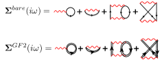
Figure 1: Upper panel: Bare second order self-energy diagrams. Lower panel: Second order self-energy diagrams evaluated self-consistently. Note that the Green’s function lines are renormalized while the interactions lines remain bare. For details see Ref. 3.

Integration of Eqs. (10) yields:

$$G_{0}\left(i\omega_{n}\right)=\left((\mu+i\omega_{n})S-F\right)^{-1}.$$ (11)

Since we now know how to write down Green’s functions for non-interacting systems, we rewrite the unknown part of the exact Green’s function by introducing the frequency-dependent self-energy, formally defined by:

$$G\left(i\omega_{n}\right)=\left(\left(\mu+i\omega_{n}\right)S-F-\Sigma\left(i\omega_{n}\right)\right)^{-1},$$ (12)

and by construction the self-energy fulfills the Dyson equation:

$$G\left(i\omega_{n}\right)=G_{0}\left(i\omega_{n}\right)+G_{0}\left(i\omega_{n}\right)\Sigma\left(i\omega_{n}\right)G\left(i\omega_{n}\right).$$ (13)

Instead of viewing these equations as a definition of the self-energy $\Sigma\left(i\omega_{n}\right)$, we can calculate this self-energy to a given order of perturbation theory in $\Delta\hat{H}=\hat{H}-\hat{H}_{0}$. Specifically, the GF2 approximation^{3, 2} uses a Hartree-Fock ansatz for $F$,

$$F_{ij} =h_{ij}+\frac{1}{2}P_{kl}\left(2v_{ijkl}-v_{ilkj}\right),$$ (14)

where an Einstein summation convention is used, summing indices that appear in pairs (here, both $k$ and $l$). The self-energy in imaginary time $\Sigma(\tau)$ is then obtained by second order perturbation theory (see Fig. (1)):

$$\Sigma_{ij}\left(\tau\right) =G_{kl}\left(\tau\right)G_{mn}\left(\tau\right)G_{pq}\left(\beta-\tau\right)v_{impk}\left(2v_{jnlq}-v_{jlnq}\right).$$ (15)

Note that $\Sigma(\tau)$ and $\Sigma(i\omega_{n})$ are connected by exactly the same Matsubara relations connecting $G(\tau)$ and $G(i\omega_{n}),$ Eqs. 7-8.

The self-consistent one-body Green’s function governs all one-body expectation values. Moreover, even the total two-body potential energy is available, by differentiation of the matrix trace (denoted by $\mbox{Tr}\left[\right]$) of the Green’s function with respect to $\tau$: $\left\langle\hat{V}\right\rangle=-\frac{1}{2}\lim_{\tau\to 0^{-}}\mbox{Tr}\left[\left((\frac{\partial}{\partial\tau}-\mu)S+h\right)G\left(\tau\right)\right]$. Hence, the total energy is:

$$\left\langle\hat{H}\right\rangle={\rm Tr}\left[hP-\frac{1}{2}\lim_{\tau\to 0^{-}}\left((\frac{\partial}{\partial\tau}-\mu)S+h\right)G\left(\tau\right)\right].$$ (16)

It is easy to show by plugging the definition of $G(\tau)$ to Eq. (16) that this total energy has convenient frequency and time forms:

$$\left\langle\hat{H}\right\rangle =\frac{1}{2}\mbox{Tr}\left[\left(h+F\right)P\right]+\frac{2}{\beta}\mbox{Re}\sum_{n}\mbox{Tr}\left[G\left(i\omega_{n}\right)\Sigma^{T}\left(i\omega_{n}\right)\right]$$ (17)

$$=\frac{1}{2}\mbox{Tr}\left[\left(h+F\right)P\right]+2\int_{0}^{\beta}\text{Tr}\left[G\left(\beta-\tau\right)\Sigma\left(\tau\right)\right]d\tau.$$

To conclude, the combination of Eqs. (9), (12), (14) and (15) along with the requirement that the density matrix describes $N_{e}$ electrons results in the following self-consistent GF2 procedure:

1. Perform a standard HF calculation and obtain a starting guess for the Fock matrix $F=F_{HF}$ and the density matrix $P=P_{HF}.$ Set $\Sigma\left(i\omega_{n}\right)=0$ for the set of $N_{\omega}$ positive Matsubara frequencies $\omega_{n},$ $n=0,1,2,\dots,N_{\omega}-1$., .

2. Given $\Sigma\left(i\omega_{n}\right)$ and $F$, find $\mu$ such that ${\rm Tr}\left[PS\right]=N_{e}$, where $P$ is given in Eq. (9) from $G(\tau=\beta^{-})$ which depends on $\mu$ through the basic definition Eq. (12).

3. Calculate $G\left(\tau\right)$ (Eq. (7)) and $P$ (Eq. (9)).

4. Calculate the Fock matrix $F$ from $P$ (Eq. (14)).

5. Calculate the self-energy $\Sigma\left(\tau\right)$ from Eq. (15) and transform is to the Matsubara frequency domain to yield $\Sigma\left(i\omega_{n}\right).$

6. Calculate the total energy$\left\langle\hat{H}\right\rangle$ from Eq. (17).

7. Repeat steps 2-6 until convergence of the density and the total energy.

Once converged, the GF2 correlation energy is defined as the difference $E_{{\rm corr}}=\left\langle\hat{H}\right\rangle-E_{{\rm HF}}$ between the converged total energy (Eq. (17)) and the initial Hartree-Fock energy, $E_{HF}=\frac{1}{2}\mbox{Tr}\left[\left(h+F_{HF}\right)P_{HF}\right]$. Note that in the first iteration GF2 yields automatically the temperature-dependent MP2 energy:

$$E_{{\rm MP2}}^{corr} =\int_{0}^{\beta}\text{Tr}\left[G_{0}\left(\beta-\tau;F_{HF}\right)\Sigma_{0}\left(\tau\right)\right]d\tau,$$ (18)

where $\Sigma_{0}\left(\tau\right)$ is that of Eq. (15) with $G_{0}$ replacing $G$. This expression reduces to the familiar MP2 energy expression at the limit $\beta\to\infty$ (zero temperature limit), when evaluated in the molecular orbital basis set that diagonalizes the matrix $F_{HF}$.

Finally, a technical point. The representation of the Green’s functions in $\tau$-space can be complicated when the energy range of the eigenvalues of $F$ is large since a function of the type $e^{-\tau\left(f-\mu\right)}/\left(1+e^{-\beta\left(f-\mu\right)}\right)$ can be spiky when $f>\mu$ and $\tau\to\beta$ or when $f<\mu$ and $\tau\to 0$. This requires special techniques for both imaginary time and frequency grids as discussed in Refs. 33, 34.

2.2 sGF2: Stochastic approach to GF2

Most of the computational steps in the above algorithm scale with system size $N$ (number of AO basis functions) as ${\rm O}\!\left(N_{SC}\times N_{\tau}\times N^{3}\right)$ where $N_{SC}$ is the number of GF2 self-consistent iterations and $N_{\tau}$ is the number of time-steps. However, the main numerical challenge in GF2 is step 5 (Eq. (15)) which scales formally as ${\rm O}\!\left(N_{SC}\times N_{\tau}\times N^{5}\right)$ making GF2 highly expensive for any reasonably sized system. This steep scaling is due to the contraction of two 4-index tensors with three Green’s function matrices.

To reduce this high complexity, we turn to the stochastic paradigm which represents the matrices $G\left(\tau\right)$ by an equivalent random average over stochastically chosen vectors. Fundamentally, this is based on resolving the identity operator. Specifically, for each $\tau$ we generate a vector $\eta^{0}$ of $N$ components randomly set to $+1$ or $-1$. Vectors at different times $\tau$ are statistically independent, but we omit for simplicity their $\tau$ labeling. Then, the key, and trivial, observation is that average of the product of different components of $\eta^{0}$ is the unit matrix, which we write symbolically as

$$\eta_{k}^{0}\eta_{l}^{0}=\delta_{kl}.$$ (19)

We emphasize that the equality in this equation should be interpreted to hold in the limit of averaging over infinitely many random vectors $\eta^{0}.$

Given this separable presentation of the unit matrix, it is easy to rewrite any matrix as an average over separable vectors. Specifically, from $\eta^{0}$ we define the two vectors:

$$\eta=\sqrt{|G\left(\tau\right)|}\eta^{0},\,\,\,\,\,\bar{\eta}=sgn\left(G\left(\tau\right)\right)\sqrt{|G\left(\tau\right)|}\eta^{0},$$ (20)

and then

$$G_{kl}\left(\tau\right)=\bar{\eta}_{k}\eta_{l}.$$ (21)

Here, the square-root matrix is $\sqrt{\left|G\left(\tau\right)\right|}=A\sqrt{\left|g\right|}A^{T}$, where $A\left(\tau\right)$ is the unitary matrix of eigenvectors and $g\left(\tau\right)$ is the diagonal matrix of eigenvalues of $G\left(\tau\right)$.

As a side note, we have a freedom to choose other vectors; specifically, any two vectors $\bar{\eta}=\bar{D}\eta^{0},\,\,\,\,\,\eta=D\eta^{0}$, will work if $\bar{D}D^{T}=G(\tau).$ In principle, we can even use the simplest choice $\bar{D}=1,\,\,\,\,\,D=G(\tau),$ corresponding to $\bar{\eta}=\eta^{0}$ and $\eta=G(\tau)\eta^{0}$. But while this latter choice has the advantage that $G(\tau)$ does not need to be diagonalized, we find that it is numerically better to use Eq. (20) as it is more balanced and therefore converges faster with the number of stochastic samples. Also note that at the first iteration, where $G(\tau)=G_{0}(\tau),$ there is no need to diagonalize $G_{0}(\tau)$ at different times, since it is obtained directly from the eigenstates of $\bar{F}$ in Eq. (10).

Going back to Eq. (20), we similarly separate the other two Green’s function matrices appearing in Eq. (15), writing them as $G_{mn}\left(\tau\right)=\bar{\xi}_{m}\xi_{n}$ and $G_{pq}\left(\beta-\tau\right)=\bar{\zeta}_{p}\zeta_{q}$. The self-energy in Eq. (15) is then

$$\Sigma_{ij}\left(\tau\right) =\bar{\eta}_{k}\bar{\xi}_{m}\bar{\zeta}_{p}v_{impk}\left(2\eta_{l}\xi_{n}\zeta_{q}v_{jnlq}-\eta_{l}\xi_{n}\zeta_{q}v_{jlnq}\right),$$ (22)

so that it is separable to a product of two terms

$$\Sigma_{ij}\left(\tau\right)=\bar{u}_{i}\left[2u_{j}-w_{j}\right],$$ (23)

where we defined three auxiliary vectors

$$\bar{u}_{i} =\bar{\eta}_{k}\bar{\xi}_{m}\bar{\zeta}_{p}v_{impk}$$

$$u_{j} =\eta_{l}\xi_{n}\zeta_{q}v_{jnlq}$$ (24)

$$w_{i} =\eta_{l}\xi_{n}\zeta_{q}v_{jlnq}.$$

The self-energy in Eq. (23) should be viewed as the average, over the stochastic vectors $\xi^{0}$, $\eta^{0}$ and $\zeta^{0},$ of the product term ($\bar{u}_{i}$ times $2u_{j}-w_{j}).$

The direct calculation of the vectors $\bar{u},\,u,\,w$ by Eq. (24) is numerically expensive once $M>30$ . We reduce the scaling by recalling the definition of $v_{jnlq}$ in Eq. (3):

$$u_{j} =\eta_{l}\xi_{n}\zeta_{q}\iint\phi_{j}\left(\boldsymbol{r}\right)\phi_{n}\left(\boldsymbol{r}\right)v\left(\left|\boldsymbol{r}-\boldsymbol{r}^{\prime}\right|\right)\phi_{l}\left(\boldsymbol{r}^{\prime}\right)\phi_{q}\left(\boldsymbol{r}^{\prime}\right)d\boldsymbol{r}d\boldsymbol{r}^{\prime}$$ (25)

$$=\iint\phi_{j}\left(\boldsymbol{r}\right)\xi\left(\boldsymbol{r}\right)v\left(\left|\boldsymbol{r}-\boldsymbol{r}^{\prime}\right|\right)\eta\left(\boldsymbol{r}^{\prime}\right)\zeta\left(\boldsymbol{r}^{\prime}\right)d\boldsymbol{r}d\boldsymbol{r}^{\prime},$$ (26)

where:

$$\eta\left(\boldsymbol{r}\right)=\eta_{l}\phi_{l}\left(\boldsymbol{r}\right),$$ (27)

and $\xi\left(\boldsymbol{r}\right)$ and $\zeta\left(\boldsymbol{r}\right)$ are analogously defined. We can therefore write

$$u_{j}=\int\phi_{j}\left(\boldsymbol{r}\right)\xi\left(\boldsymbol{r}\right)v_{\eta\zeta}\left(\boldsymbol{r}\right)d\boldsymbol{r},$$ (28)

where

$$v_{\eta\zeta}\left(\boldsymbol{r}\right)\equiv\int v\left(\left|\boldsymbol{r}-\boldsymbol{r}^{\prime}\right|\right)\eta\left(\boldsymbol{r}^{\prime}\right)\zeta\left(\boldsymbol{r}^{\prime}\right)d\boldsymbol{r}^{\prime}$$ (29)

is the Coulomb potential corresponding to the random charge distribution $\eta\left(\boldsymbol{r}\right)\zeta\left(\boldsymbol{r}\right)$. Similar expressions apply for $\bar{u}_{i}$ and $w_{j}$.

Equations (28)-(29) are performed numerically using FFT methods on a 3D Cartesian grid with $N_{g}$ grid points, so Eq. (29) is calculated with ${\rm O}\!\left(N_{g}\log N_{g}\right)$ operations. Since the AO basis functions $\phi_{i}\left(\boldsymbol{r}\right)$ are local in 3D space, the calculations of $\eta\left(\boldsymbol{r}\right)$, $\xi\left(\boldsymbol{r}\right)$ and $\zeta\left(\boldsymbol{r}\right)$ in Eq. (27) scale linearly with system size.

Eq. (23) gives an exact expression for $\Sigma_{ij}\left(\tau\right),$ as an expected value over formally an infinite number of stochastic orbitals $\eta^{0}$, $\xi^{0}$ and $\zeta^{0}$. Actual calculations use a finite number $I$ of “stochastic iterations”, where in each such iteration a set of stochastic vectors $\eta^{0}$, $\xi^{0}$ and $\zeta^{0}$ (different at each $\tau)$ is generated and $\Sigma_{ij}\left(\tau\right)$ is averaged over them. The overall scaling of this step is therefore $I\times N_{\tau}\times\left(N_{g}\log N_{g}+N^{2}\right)$. We note that the typical values of $N_{\tau}$ and $I$ are in the hundreds, see the discussion of the stochastic error below.

Finally, we note that while the stochastic vectors ($\eta^{0}$,$\zeta^{0},\xi^{0}$) are statistically independent for each time point $\tau$, the same $\tau-$dependent vectors are used at each GF2 iteration, making it possible to converge these iterations.

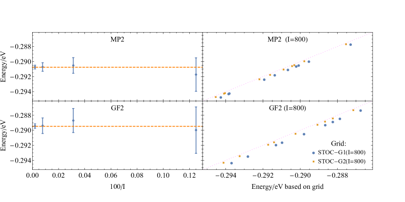
Figure 2: MP2 and GF2 correlation energies per electron for a linear $\text{H}_{10}$ system with nearest neighbor spacing of 1ￜ. Left panels: the DET (deterministic) correlation energies (dashed horizontal lines) are well within the $I$-dependent error-bars $\bar{E}\pm 2\sigma$ of the STOC-NG calculations, where $\bar{E}$ and $\sigma$ are the average and standard deviation of the correlation energy calculated in 10 statistically independent runs. Right panels: a correlation plot of pairs of stochastically ($I=800$) estimated correlation energies: $\left(E_{STOC-G1\left(800\right)},E_{STOC-NG\left(800\right)}\right)_{i}$ as blue dots and $\left(E_{STOC-G2\left(800\right)},E_{STOC-NG\left(800\right)}\right)_{i}$ as orange dots, $i=1,\dots,10$. The diagonal dotted line represents the perfect correlation $E_{STOC-G1\,or\,2}=E_{STOC-NG}$.

3 Results

3.1 Systems and specifics

The algorithm was tested on linear hydrogen chains, $(H_{M}$) a nearest neighbor distance of $1$ￜ, for several sizes: $M=10,100,300$ and $1000$. The linearity was for convenience and we emphasize that it does not play any role in the algorithm. The smallest chain was used to demonstrate the convergence of the approach to the basis-set deterministic values, and the other three calculations were used to study the dependence of the algorithm on system size.

In all calculations, an STO-3G basis was used, so that in this case $N=M$ and obviously the number of electrons is also $N_{e}=M$. A periodic spatial grid of $0.5a_{0}$ spacing was used to represent the wave functions, and the grids contained $10\times 10$ points in the direction orthogonal to chain and between 60 and 4000 points along the chain, depending on system size. For the smallest system ($H_{10}$) a finer, bigger grid was also used, as detailed below.

Other, technical details:

• Periodic images were screened using the method of Ref. 35.

• The inverse temperature was $\beta=50E_{h}^{-1}$.

• A Chebyshev-type imaginary-time grid with 128 time points was employed using a spline-fit method ^{33, 34} for the frequency-to-time conversions of $G(i\omega_{n})$ and $\Sigma(i\omega_{n})$ and for the evaluation of the two-body energy.

3.2 Small system

In our GF2 and MP2 algorithm, we make two types of numerical discretizations. First, we use a finite number (labeled $I$) of stochastic iterations to sample the self-energy, so we must show convergence as $I$ grows. Second, we use grids for bypassing the need to sum over ${\rm O\!}\left(N^{4}\right)$ two-electron integrals, hence we need to demonstrate convergence with respect to grid quality. We therefore examine in this section a small system, linear $\text{H}_{10}$, and make four types of GF2/MP2 correlation energy calculations:

• DET: fully deterministic calculations based on the analytical 2-electron integrals;

• STOC($I$)-NG: stochastic calculations based on $I$ stochastic iterations and on the analytical two electron integrals;

• STOC($I$)-G1 and STOC($I$)-G2: stochastic calculations based on $I$ stochastic iterations and on a 3D grid. Here, G1 is the same type of grid we use for the larger calculations, and includes $10\times 10\times 60$ points with a spacing $h=0.5a_{0}$. G2 is somewhat denser and covers more space, with $16\times 16\times 100$ points and $h=0.4a_{0}$.

Our strategy is to first show that STOC-NG($I$) converges to the deterministic set (DET) as $I$ grows. Then we show that for a given number of stochastic orbitals, $I=800,$ both grid results are quite close to the non-grid result, and that the somewhat better second grid (STOC($I=800$)-G2 leads to extremely close results to the non-grid values (STOC($I=800$)-NG), so that the convergence with grid is very rapid.

We repeat the STOC-NG calculation 10 times determining the average correlation energy $\bar{E}$ and its standard deviation $\sigma$ as a function of $I$. The results are shown in the left panels of Fig. 2 as error-bars at $\bar{E}\pm\sigma$, which shrink approximately as $1/\sqrt{I}$ and which include the DET result, represented as dashed horizontal lines, showing very small or no bias. For MP2, a bias in the stochastic calculations is not expected since the correlation energy is calculated linearly from the first iteration of the self-energy $\Sigma_{0}$ (Eq. (18)). But for GF2 such a bias may form since the the “noisy” self-energy is used non-linearly to update the Green’s function in Eq. (12). However, for this small $N=10$ system the stochastic MP2 and GF2 energies do not exhibit a noticeable bias. We discuss the bias in larger systems below.

Next, we asses the errors associated with using grid calculations replacing the analytical 2-electron integration. In both right panels of Fig. 2 we show 10 blue dots, each corresponding to a pair of stochastic energies $\left(E_{STOC-G1\left(800\right)},E_{STOC-NG\left(800\right)}\right)_{i}$ , $i=1,\dots,10$, both calculated with the same random seed $s_{i}$ (of course $s_{i}$ and $s_{j}$ are statistically independent). We also show 10 orange dots, each corresponding to a pair of stochastic energies $\left(E_{STOC-G2\left(800\right)},E_{STOC-NG\left(800\right)}\right)_{i}$, also calculated with the same seed $s_{i}$ as before. The use of the same seeds for each pair of blue and orange dots allows for comparison of the grid error (which is the horizontal distance of a point from the diagonal) without worrying about the larger statistical error, seen as the spread of the results along the diagonal. We see that the grid error decreases significantly when moving from G1 to G2, but even the error for G1 is already very small (about 0.5meV per electron).

3.3 Larger systems

In the small system considered above the bias was not noticeable and here we examine the bias in larger systems. In Fig. 3 we show the STOC-G1(I) correlation energies in three specific systems composed of $N=100,300$ and $1000$ hydrogen atoms placed on a straight line with a nearest neighbor spacing of $1$ ï¿œ.

We first study the MP2 correlation energy of each system, appearing in the lower energy range in the figure. The starting point of the GF2 calculation is the Hartree-Fock $F_{HF}$ and $P_{HF}$ matrices, so the MP2 energy is half the correlation energy of the first self-consistent iteration (see Eqs. (17) and (18)). The statistical errors in MP2 are pure fluctuations, a random number distributed normally with zero average and with standard deviation given by $\sigma_{0}/\sqrt{I}$ where $\sigma_{0}$ is independent of $I$ but shrinks with chain length: $\sigma_{0}\propto 1/\sqrt{L}$, exhibiting “self averaging”. ¹⁸ The stochastic MP2 errors are very small and decrease with system size, so for $N=1000$ the standard deviation of the $I=800$ iteration calculation is 0.07% of the total correlation energy. For perspective, note that (deterministic) errors of larger or similar magnitude are present in linear scaling local or divide and conquer MP2 methods with density fitting. ^{36, 37}

Next, we discuss the stochastic estimates of the self-consistent GF2 correlation energies. These exhibit statistical errors with two visible components. The first is a fluctuation, similar in nature to that of the MP2 calculation, and the second component is a bias which decreases as $I$ grows. In fact, we expect the bias to asymptotically decrease inversely with $I$, so we fit the numerical GF2 results to a straight line in $I^{-1}$. Table 1 shows the estimate of the correlation energies, the fluctuation and the bias as a function of the number of stochastic orbitals. The results are highly accurate, for example when $I=800$ is used for the largest system ($N=1000$), the errors in MP2 and in GF2 are smaller than 0.1%.

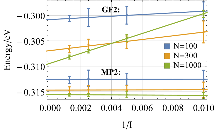
Figure 3: Statistical estimates of the MP2 and GF2 correlation energies per electron for three linear chains with $N=100$, $300$ and $1000$ H atoms as described in the text, as a function of the inverse number of sets of stochastic orbitals $I$. The results are shown as error bars, where the center of each error bar is the average and its width is the standard deviation of the correlation energy estimates from 10 statistically independent runs, each employing $I$ sets of stochastic orbitals. The lines are linear regression fits to the data and uncertainties.

$N$	MP2 Energy (eV)		GF2 Energy (eV)
	$E\left(N,I\right)$	$I=800$	$E\left(N,I\right)$	$I=800$
100	$-0.3126\pm 0.025I^{-1/2}$	$-0.3127(9)$	$-0.3008+0.16I^{-1}\pm 0.025I^{-1/2}$	$-0.3007(9)$
300	$-0.3148\pm 0.015I^{-1/2}$	$-0.3148(5)$	$-0.3069+0.36I^{-1}\pm 0.020I^{-1/2}$	$-0.3067(7)$
1000	$-0.3157\pm 0.007I^{-1/2}$	$-0.3157(2)$	$-0.3094+0.98I^{-1}\pm 0.010I^{-1/2}$	$-0.3094(3)$

Table 1: The statistical estimate of the MP2 and GF2 energies per electron of the linear hydrogen chains $\text{H}_{N}$, based on runs with up to $I=800$ stochastic samplings. For MP2 there is no bias and the error is a only statistical fluctuation which for $I=800$ is very small, on the order of 0.1% of the correlation energy or better. For GF2 the statistical fluctuation is similarly tiny, and there is a bias (depending to leading order on $I^{-1})$ that grows with $N$, and therefore $I$ should be similar to $N$ or larger.

Timings. The measured overall CPU time for the stochastic self-energy calculation (performed on a XEON system) can be expressed as

$$T^{\Sigma}\approx 2.5\times N\times N_{\tau}\times I\times 10^{-7}hr,$$ (30)

where, as mentioned, $N$ is the number of electrons and $I$ the number of stochastic orbitals in the system. The MP2 wall time calculation is essentially equal to the self-energy time divided by the number of cores $n_{CORES}$, since the parallelization has negligible overhead:

$$T_{\text{wall}}^{MP2}\approx\frac{T^{\Sigma}}{n_{CORES}}.$$ (31)

GF2 involves an additional step, where the Green’s function is constructed from the self-energy and this step scales cubically with system size. Furthermore, there are $N_{SC}$ self-consistent iterations. The total time is therefore found to be:

$$T_{\text{wall}}^{GF2} \approx N_{SC}\frac{\left(1.7\times N^{3}\times N_{\tau}\text{$\times$1$0^{-11}$hr}+T^{\Sigma}\right)}{n_{CORES}}.$$

For the $\text{H}_{1000}$ system, with $I=800$ stochastic orbitals, the MP2 calculation takes $T_{\text{wall}}^{MP2}=24\text{hr}/n_{CORES}$, i.e. about $30$min when using 48 cores.

The GF2 calculation for this same system involves $N_{SC}=12$ iterations and a cubic part which takes about 2 core-hours per iteration, i.e., the cubic part is still an order of magnitude smaller than the self-energy sampling time for this system size. The wall time is therefore $T_{\text{wall}}^{GF2}=6.5\text{hr}$ with 48 cores.

For the $\text{H}_{300}$ system we find $T_{\text{wall}}^{MP2}=12$min and $T_{\text{wall}}^{GF2}=2\text{hr}$ while for $\text{H}_{100}$ we have $T_{\text{wall}}^{MP2}=3.5\text{min}$ and $T_{\text{wall}}^{GF2}=40{\rm min}$.

Note that these timings are for a single calculation. The error estimation uses, as mentioned, ten completely independent runs, and therefore took 10 times longer.

For comparison, we note that the CPU time for the deterministic calculation in the $\text{H}_{100}$ system takes $45$ min. on a single core, which is 4 times faster than the stochastic calculation. Since the deterministic algorithm scales steeply as $O\left(N^{5}\right)$, the crossover occurs already at $\text{H}_{150}$ and at $\text{H}_{1000}$ the deterministic calculation would take $\frac{10^{4}-10^{5}}{n_{CORES}}$ wall time hours per SCF iteration, compared to $\frac{24}{n_{CORES}}$ hours for the stochastic calculations.

3.4 Born Oppenheimer potential curves

Potential energy curves can be calculated by correlated sampling, where at each new nuclear configuration one employs the same set of stochastic orbitals $\eta_{0},$$\,\xi_{0}$ and $\zeta_{0}$ for the self-energy estimation. For demonstration, the HF, MP2 and GF2 Born Oppenheimer potentials of the $\text{H}_{100}$ system are shown in Fig. 4 as a function of the displacement of atom no. 25 (counting from the left). In all three methods the most stable position of the atom is at $\sim-0.1a_{0}$, slightly displaced towards the nearest chain end. HF theory produces an energy potential with large variations of up to $1.5$eV and large vibrational frequencies of order of 3.4eV. The MP2 curve is much smoother and the vibrational frequencies reduces to $\sim 2.4$eV while the GF2 energy curve is considerably flatter, predicting a vibrational frequency of $\sim 1.0$ eV.

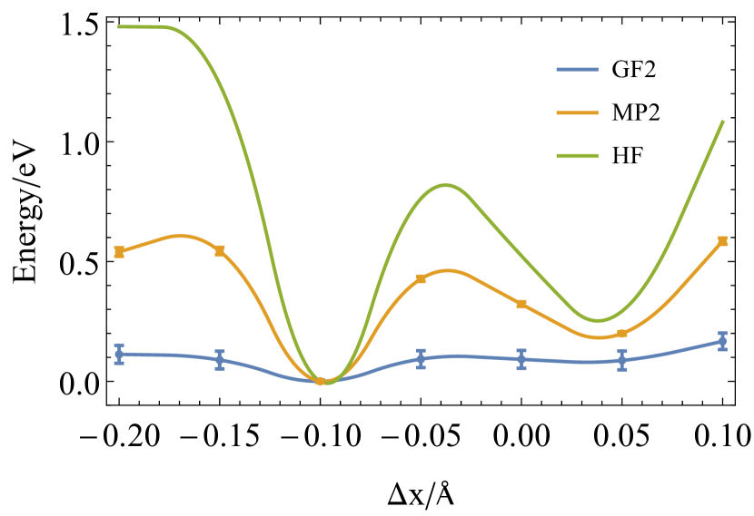
Figure 4: Hartree-Fock, MP2 and GF2 potential energy curves for the energy change in the displacement $\Delta x$ of atom no. 25 in the 100 H chain.

4 Summary and Conclusions

The problem we addressed here is the reduction of the the steep ${\rm O({\it N}^{5})}$ scaling associated with the implementation of self-consistent GF2 calculations. We developed an effective way to reduce complexity to ${\rm O({\it N}^{3})}$ by using stochastic techniques for calculating the self-energy. A detailed derivation was given along with a specific algorithm. The sampling error in the overall algorithm was studied for linear $\text{H}_{N}$ systems, and the simulation showed that the stochastic errors in the correlation energies can be controlled to less than 0.1% for very large systems. While the studied systems were linear, the algorithm makes no use of the linearity and applies equally well to any geometry.

As a byproduct, since the first step in GF2 is equivalent to MP2, we obtain a stochastic MP2 method (sMP2) performed on top of an existing HF calculation. This approach too has a formal complexity of ${\rm O\!}\left(N^{5}\right)$ which is reduced here to linear ${\rm O({\it N})}$, except for a single overall Fock-matrix diagonalization which is often available from the underlying HF or DFT ground-state calculation. The errors in this well-scaling stochastic MP2 method are comparable to those of local MP2 approaches used in quantum chemistry.

For GF2, the method has two main stages. The first stage, as in the MP2 case, is a linear scaling calculation of the self-energy. This self-energy is then used in the second stage to construct the Green’s function, at an ${\rm O\!}\left(N^{3}\right)$ cost. A complication arises in GF2 due to this second stage (but not in MP2!), where the self-energy enters non-linearly into the expression for the Green’s function. This non-linearity gives rise to a noticeable bias which is proportional to the system size $N$. To overcome this bias the number of stochastic orbitals $I$ used in the first step must be increased in proportion to the system size $N$, and hence the self-energy calculation in GF2 attains an ${\rm O\!}\left(N^{2}\right)$ scaling. The overall scaling of the GF2 calculation is unaffected by this bias problem and remains ${\rm O\!}\left(N^{3}\right)$.

The present calculations give a fully self-consistent Green’s function method for a large system with a thousand electrons described by a full quantum chemistry Hamiltonian. Moreover, we demonstrated that the splitting of matrices by a random average over stochastically chosen vectors leads to small variance and that relatively few Monte Carlo samples already yield quite accurate correlation energies. The reason for this excellent sampling dependence is two-fold: the stochastic sampling inherently acts only in the space of atomic orbitals while the actual spatial integrals (Eq. (29)) are evaluated using a deterministic, numerically exact calculation; in addition, since the Green’s function matrices are smooth in imaginary time, different random vectors can be used at each imaginary-time point thereby enhancing the stochastic sampling efficiency.

We have shown that both sMP2 and sGF2 are suitable for calculating potential energy curves or surfaces. Interestingly, for the $\text{H}_{N}$ systems the potential curve is much smoother and flatter than in HF or MP2.

As for future applications, we note that sGF2 and sMP2 methods are automatically suitable for periodic systems, as all the deterministic steps and the time-frequency transforms are very efficient when done in the reciprocal $(k)$ space. The only additional detail is that in periodic systems one needs to choose the random vectors to be in $k$-space and then convert them to real-space, as detailed in an upcoming article.

Finally, we also note that, beyond the results presented here, it should also be possible to achieve further reduction of the stochastic error with an embedded fragment approach, analogous to self-energy embedding approaches, where a deterministic self-energy is calculated for embedded saturated fragments as introduced for stochastic DFT applications. ^{19, 20}

Discussions with Eran Rabani are gratefully acknowledged. D.N. was supported by NSF grant DMR-16111382, R.B. acknowledges support by BSF grant 2015687 and D.Z. was supported by NSF grant CHE-1453894.

References

- Baym 1962 Baym, G. Self-consistent approximations in many-body systems. Phys. Rev. 1962, 127, 1391
- Dahlen and van Leeuwen 2005 Dahlen, N. E.; van Leeuwen, R. Self-consistent solution of the Dyson equation for atoms and molecules within a conserving approximation. The Journal of Chemical Physics 2005, 122
- Phillips and Zgid 2014 Phillips, J. J.; Zgid, D. Communication: The description of strong correlation within self-consistent Green’s function second-order perturbation theory. J. Chem. Phys. 2014, 140, 241101
- Phillips et al. 2015 Phillips, J. J.; Kananenka, A. A.; Zgid, D. Fractional charge and spin errors in self-consistent Green’s function theory. J. Chem. Phys. 2015, 142, 194108
- Hedin 1965 Hedin, L. New Method for Calculating the One-Particle Green’s Function with Application to the Electron-Gas Problem. Phys. Rev. 1965, 139, A796–A823
- Fetter and Walecka 1971 Fetter, A. L.; Walecka, J. D. Quantum Thoery of Many Particle Systems; McGraw-Hill: New York, 1971; p 299
- Onida et al. 2002 Onida, G.; Reining, L.; Rubio, A. Electronic excitations: density-functional versus many-body Green’s-function approaches. Rev. Mod. Phys. 2002, 74, 601–659
- Rusakov and Zgid 2016 Rusakov, A. A.; Zgid, D. Self-consistent second-order Green’s function perturbation theory for periodic systems. J. Chem. Phys. 2016, 144, 054106
- Welden et al. 2016 Welden, A. R.; Rusakov, A. A.; Zgid, D. Exploring connections between statistical mechanics and Green’s functions for realistic systems: Temperature dependent electronic entropy and internal energy from a self-consistent second-order Green’s function. The Journal of Chemical Physics 2016, 145, 204106
- Kananenka et al. 2015 Kananenka, A. A.; Gull, E.; Zgid, D. Systematically improvable multiscale solver for correlated electron systems. Phys. Rev. B 2015, 91, 121111
- Lan et al. 2015 Lan, T. N.; Kananenka, A. A.; Zgid, D. Communication: Towards ab initio self-energy embedding theory in quantum chemistry. The Journal of Chemical Physics 2015, 143
- Nguyen Lan et al. 2016 Nguyen Lan, T.; Kananenka, A. A.; Zgid, D. Rigorous Ab Initio Quantum Embedding for Quantum Chemistry Using Green’s Function Theory: Screened Interaction, Nonlocal Self-Energy Relaxation, Orbital Basis, and Chemical Accuracy. J. Chem. Theory Comput. 2016, 12, 4856–4870
- Lan and Zgid 2017 Lan, T. N.; Zgid, D. Generalized Self-Energy Embedding Theory. The Journal of Physical Chemistry Letters 2017, 8, 2200–2205, PMID: 28453934
- Zgid and Gull 2017 Zgid, D.; Gull, E. Finite temperature quantum embedding theories for correlated systems. New J. Phys. 2017, 19, 023047
- Thom and Alavi 2007 Thom, A. J.; Alavi, A. Stochastic perturbation theory: A low-scaling approach to correlated electronic energies. Phys. Rev. Lett. 2007, 99, 143001
- Kozik et al. 2010 Kozik, E.; Van Houcke, K.; Gull, E.; Pollet, L.; Prokof’ev, N.; Svistunov, B.; Troyer, M. Diagrammatic Monte Carlo for correlated fermions. EPL (Europhysics Letters) 2010, 90, 10004
- Willow et al. 2013 Willow, S. Y.; Kim, K. S.; Hirata, S. Stochastic evaluation of second-order Dyson self-energies. The Journal of chemical physics 2013, 138, 164111
- Baer et al. 2013 Baer, R.; Neuhauser, D.; Rabani, E. Self-Averaging Stochastic Kohn-Sham Density-Functional Theory. Phys. Rev. Lett. 2013, 111, 106402
- Neuhauser et al. 2014 Neuhauser, D.; Baer, R.; Rabani, E. Communication: Embedded fragment stochastic density functional theory. J. Chem. Phys. 2014, 141, 041102
- Arnon et al. 2017 Arnon, E.; Rabani, E.; Neuhauser, D.; Baer, R. Equilibrium configurations of large nanostructures using the embedded saturated-fragments stochastic density functional theory. J. Chem. Phys. 2017, 146, 224111
- Baer and Neuhauser 2012 Baer, R.; Neuhauser, D. Communication: Monte Carlo calculation of the exchange energy. J. Chem. Phys. 2012, 137, 051103–4
- Baer and Rabani 2012 Baer, R.; Rabani, E. Expeditious stochastic calculation of multiexciton generation rates in semiconductor nanocrystals. Nano Lett. 2012, 12, 2123
- Neuhauser et al. 2013 Neuhauser, D.; Rabani, E.; Baer, R. Expeditious Stochastic Approach for MP2 Energies in Large Electronic Systems. J. Chem. Theory Comput. 2013, 9, 24–27
- Ge et al. 2013 Ge, Q.; Gao, Y.; Baer, R.; Rabani, E.; Neuhauser, D. A Guided Stochastic Energy-Domain Formulation of the Second Order Møller–Plesset Perturbation Theory. J. Phys. Chem. Lett. 2013, 5, 185–189
- Takeshita et al. 2017 Takeshita, T. Y.; de Jong, W. A.; Neuhauser, D.; Baer, R.; Rabani, E. A Stochastic Formulation of the Resolution of Identity: Application to Second Order M o ller-Plesset Perturbation Theory. arXiv preprint arXiv:1704.02044 2017,
- Neuhauser et al. 2013 Neuhauser, D.; Rabani, E.; Baer, R. Expeditious Stochastic Calculation of Random-Phase Approximation Energies for Thousands of Electrons in Three Dimensions. J. Phys. Chem. Lett. 2013, 4, 1172–1176
- Neuhauser et al. 2014 Neuhauser, D.; Gao, Y.; Arntsen, C.; Karshenas, C.; Rabani, E.; Baer, R. Breaking the Theoretical Scaling Limit for Predicting Quasiparticle Energies: The Stochastic G W Approach. Phys. Rev. Lett. 2014, 113, 076402
- Vlcek et al. 2017 Vlcek, V.; Rabani, E.; Neuhauser, D.; Baer, R. Stochastic GW calculations for molecules. arXiv preprint arXiv:1612.08999 2017,
- Vlček et al. 2017 Vlček, V.; Baer, R.; Rabani, E.; Neuhauser, D. Self-consistent band-gap renormalization GW. arXiv preprint arXiv:1701.02023 2017,
- Gao et al. 2015 Gao, Y.; Neuhauser, D.; Baer, R.; Rabani, E. Sublinear scaling for time-dependent stochastic density functional theory. J. Chem. Phys. 2015, 142, 034106
- Neuhauser et al. 2015 Neuhauser, D.; Rabani, E.; Cytter, Y.; Baer, R. Stochastic Optimally-Tuned Ranged-Separated Hybrid Density Functional Theory. J. Phys. Chem. A 2015,
- Rabani et al. 2015 Rabani, E.; Baer, R.; Neuhauser, D. Time-dependent stochastic Bethe-Salpeter approach. Phys. Rev. B 2015, 91, 235302
- Kananenka et al. 2016 Kananenka, A. A.; Phillips, J. J.; Zgid, D. Efficient temperature-dependent Green’s functions methods for realistic systems: Compact grids for orthogonal polynomial transforms. J. Chem. Theory Comput. 2016, 12, 564–571
- Kananenka et al. 2016 Kananenka, A. A.; Welden, A. R.; Lan, T. N.; Gull, E.; Zgid, D. Efficient Temperature-Dependent Green’s Function Methods for Realistic Systems: Using Cubic Spline Interpolation to Approximate Matsubara Green’s Functions. J. Chem. Theory Comput. 2016, 12, 2250–2259
- Martyna and Tuckerman 1999 Martyna, G. J.; Tuckerman, M. E. A reciprocal space based method for treating long range interactions in ab initio and force-field-based calculations in clusters. J. Chem. Phys. 1999, 110, 2810–2821
- Werner et al. 2003 Werner, H. J.; Manby, F. R.; Knowles, P. J. Fast linear scaling second-order Moller-Plesset perturbation theory (MP2) using local and density fitting approximations. J. Chem. Phys. 2003, 118, 8149–8160
- Baudin et al. 2016 Baudin, P.; Ettenhuber, P.; Reine, S.; Kristensen, K.; Kjærgaard, T. Efficient linear-scaling second-order Møller-Plesset perturbation theory: The divide–expand–consolidate RI-MP2 model. The Journal of chemical physics 2016, 144, 054102