MMGAN: Manifold-Matching Generative Adversarial Network

Abstract

It is well-known that GANs are difficult to train, and several different techniques have been proposed in order to stabilize their training. In this paper, we propose a novel training method called manifold-matching, and a new GAN model called manifold-matching GAN (MMGAN). MMGAN finds two manifolds representing the vector representations of real and fake images. If these two manifolds match, it means that real and fake images are statistically identical. To assist the manifold-matching task, we also use i) kernel tricks to find better manifold structures, ii) moving-averaged manifolds across mini-batches, and iii) a regularizer based on correlation matrix to suppress mode collapse.

We conduct in-depth experiments with three image datasets and compare with several state-of-the-art GAN models. 32.4% of images generated by the proposed MMGAN are recognized as fake images during our user study (16% enhancement compared to other state-of-the-art model). MMGAN achieved an unsupervised inception score of 7.8 for CIFAR-10.

I Introduction

Generative adversarial networks (GANs) [7] have been recently proposed to generate synthetic images. However, it had been shown that it is notoriously difficult to train GANs due to several reasons [2]. One of the main difficulties arise by ill-designed loss functions and zero gradients.

Researchers have proposed several variations to solve such a difficult training process [9, 3, 20]. In this paper, we propose a new loss function based on manifold-matching. The manifold hypothesis puts forth the proposition that natural data will form manifolds in the embedding space [16]. From this perspective, it is likely that there exist two distinct manifolds: one formed by real data samples and another formed by generated samples. Our proposed method trains the generator $G$ with a specially designed loss function to match the two manifolds. Particularly in this paper, we assume a spherical manifold for various computational conveniences that it affords, such as kernel tricks. Furthermore, a spherical manifold can be described by a center point and its radius, making it easy to check if two spherical manifolds match. We can easily apply kernel tricks to spherical manifolds [10], by representing a space mapping via a kernel, thereby being able to apply the mapping without explicitly performing the mapping operation. Thus, our definition of manifold-matching accompanies space mappings (i.e., kernel tricks) to find more reliable manifold representations of images. This approach is better than using manifolds in the original feature space. The proposed manifold-matching GAN (MMGAN) is named after this notion of manifold-matching.

Training with mini-batches is the standard way to train neural networks. We use the exponentially weighted moving average to find center points and radii of two manifolds across multiple mini-batches and match them. This is more stable than the local manifold-matching in a mini-batch.

We also propose a regularization term to enhance diversity in generated samples, which allows MMGAN to avoid mode collapsing, a well-known problem in GANs. That is, the manifold of generated samples will collapse to a point if all the samples are too similar.

We implement the proposed MMGAN on top of the deep convolutional GAN (DCGAN) [17] and improved GAN (IGAN)  [20]. DCGAN and IGAN have similar neural network architectures, but IGAN uses a more advanced training method than DCGAN. We replace the loss functions of the two state-of-the-art GAN models with our proposed manifold-matching loss.

To evaluate the performance, we use three popular image datasets: MNIST [13], CelebA [14], and CIFAR-10 [12]. Our experiments shows that MMGAN performs as good as popular GAN models or sometimes even better than them.

II Related Work and Preliminaries

II-A Generative Adversarial Networks (GANs)

The following minimax game equation describes the core idea of GANs [7]. Two players, a discriminator $D$ and a generator $G$, in the zero-sum minimax game are alternately trained by the following objective:

$$\min_{G}\max_{D}V(G,D)= \mathbb{E}[\log D(x)]_{x\sim p_{data}(x)}$$ (1)

$$+\mathbb{E}[\log(1-D(G(z)))]_{z\sim p(z)},$$

where $p(z)$ is a prior distribution, $G(z)$ is a generator function, and $D(\cdot)$ is a discriminator function whose output spans $[0,1]$. $D(x)=0$ (resp. $D(x)=1$) indicates that the discriminator $D$ classifies a sample $x$ as generated (resp. real).

Previously, it was shown that it is possible that a manifold $M_{R}$ representing real data samples transversely intersects with another manifold $M_{G}$ representing samples generated by the generator $G$ during the training process [2]. This describes the main intuition behind why the discriminator $D$ becomes really strong (because it is relatively easy to build such a classifier that clearly distinguishes two transversely intersecting manifolds in an ambient space), which deteriorates the entire learning process of GANs.

II-B Other GAN Models

In Wasserstein GANs (WGANs) [3], the distance between the target distribution $p_{data}(x)$ and the generated sample distribution $p_{g}(x)$ is used in the loss function. When the loss function is minimized, the two distributions become identical (e.g., $p_{data}(x)=p_{g}(x)$). However, WGANs are known to be unstable if the gradients of the loss function are large. Therefore, they clip weights if they are too large after each stochastic gradient descent update.

In [5, 15], new distance metrics were proposed. The popular Wasserstein metric is a special case of the integral probability metric (IPM) of [15] and the energy distance of  [5] shows unbiased sum gradients. Both metrics show no less performance than the Wasserstein distance.

IGANs [20] proposed several heuristics to better train GANs: one is feature matching, and the other is mini-batch discrimination. In particular, IGANs is considered the best generative model for various image datasets [8], and it has achieved a high inception score (see Section VII-A for its description) for CIFAR-10 [20]. CVAE-GAN [4], EBAGN [23], and some others [11] extended the concept of feature matching of IGAN to pairwise feature matching and some other different feature matching concepts. These approaches are similar to our method. However, our MMGAN considers not only features but also many other factors such as manifold, kernel trick, moving average, and correlation regularization.

On the other hand, auto-encoders have been integrated with GANs. In adversarial generator-encoder networks [22], the authors proposed an adversarial architecture between an encoder and a generator, in order to match the data distributions of real and fake images. They showed that the encoder-generator game is advantageous in matching distributions. $\alpha$-GAN is one of the most recent auto-encoding GANs. It uses variational inference for training, where the intractable likelihood function is replaced by a synthetic likelihood and the unknown posterior distribution is replaced by an implicit function. Afterwards, the variational auto-encoder and the generative adversarial network can be successfully merged.

There exist many other GAN architectures. However, we primarily compare our proposed model with IGAN, DCGAN, and auto-encoding GANs, considering their popularity and influence on numerous GAN variants. For image generation tasks, most of the GAN models use the discriminator and generator neural network architectures proposed by DCGAN, and among them, IGAN is considered as the state-of-the-art for several image datasets [8].

III Manifold-Matching GAN

In this section, we first describe the main idea of manifold-matching, and then the proposed manifold-matching GAN (MMGAN).

III-A Manifold-Matching

Figure 1: Yellow points represent vector representations of data samples in a feature space. A manifold is represented by a sphere in the same feature space when $\varphi(s)=s$. A red point represents the centroid of the yellow points. The best manifold representing yellow points should minimize the sum of errors highlighted in red dotted lines.

Let $\mathcal{Y}=\{\mathbf{y_{1}},\mathbf{y_{2}},\cdots,\mathbf{y_{n}}\}$ (resp. $\mathcal{X}=\{\mathbf{x_{1}},\mathbf{x_{2}},\cdots,\mathbf{x_{n}}\}$) be the set of $d$-dimensional vector representations of real samples (resp. generated samples) — we use bold font to denote vectors, and thus, $\mathbf{x}$ is a vector representation of a sample $x$. Note that we can extract these vector representations from the last layer of the discriminator.

Given a set $\mathcal{S}$ of $n$ points or vectors (e.g., $\mathcal{S}=\{\mathbf{s_{1}},\mathbf{s_{2}},\cdots,\mathbf{s_{n}}\}$), let $M_{S}$ be a manifold representing these points. For instance, $n$ points can be described by a sphere of centroid $\mathbf{c}$ and radius $\ell$ as follows:

$$\|\varphi(\mathbf{c})-\varphi(\mathbf{s_{i}})\|^{2}_{2}=\ell^{2},$$ (2)

where $\mathbf{s_{i}}\in\mathcal{S}$ and $\varphi(\cdot)$ is a space mapping function.

Note that our manifold definition is not a simple sphere in the original feature space but a distorted sphere after the space mapping. The key point is which space mapping we will use. It is not easy and might take a lot of time to find the best manifold that describes the set $\mathcal{S}$ without any errors through a mapping $\varphi$. To this end, existing methods such as manifold learning [19] can be adopted. For instance, a projection matrix that projects vector representations onto a low-dimensional sphere and preserves distances in the original space within local neighborhoods can be learned. However, we do not adopt this approach because it will increase the training time. Instead, we use several popular kernels equivalent to space mappings. This kernel trick enables us to minimize computational overheads.

For the sake of simplicity, in this section, let us assume the simplest mapping function $\varphi(x)=x$. We describe other mappings in Section IV.

With $\varphi(s)=s$, the best manifold is achieved when its center is the centroid $\mathbf{c}$ of $n$ points, and the radius is the mean distance from the centroid to $n$ points. This manifold minimizes the error, as shown in Figure 1, where the error is defined as the minimum distance from the points to the manifold (i.e., in this case, to the surface of a sphere).

Proposition 1.

Given $n$ points in $d$-dimensional space, let us define its centroid $\mathbf{c}$ as

$$\mathbf{c}=\frac{\sum_{i}{s_{i}}}{n}.$$ (3)

Then, the centroid $\mathbf{c}$ minimizes the sum of squared distances to all the points, which is a well-known property.

Proposition 2.

Given $n$ points and their centroid $\mathbf{c}$, let us define the radius $\ell$ as

$$\ell=\frac{\|\mathbf{c}-\mathbf{s_{i}}\|_{2}}{n}.$$ (4)

Then, the radius $\ell$ minimizes the sum of squared errors from the manifold to all the points.

manifold-matching involves checking how similar $M_{\mathcal{Y}}$ and $M_{\mathcal{X}}$ are to each other. If these two manifolds are identical, we can effectively say that $p_{data}=p_{g}$ from the perspective of the discriminator (because the vector representations are obtained from the last layer of the discriminator). We use the following criteria to check if the two manifolds match.

Definition 1 (manifold-matching Condition).

Two sphere manifolds $M_{\mathcal{Y}}$ and $M_{\mathcal{X}}$ are identical if their centroids and radii are the same. For sphere manifolds, we check if $\|\mathbf{c_{M_{\mathcal{Y}}}}-\mathbf{c_{M_{\mathcal{X}}}}\|_{2}=0$ and $|\ell_{M_{\mathcal{Y}}}-\ell_{M_{\mathcal{X}}}|=0$.

III-B Manifold-Matching GAN

Figure 2: Discriminator $D$. $D(\mathrm{x})$ is computed after the last sigmoid activation. Vector representations of images are obtained by vectorizing the feature map marked in yellow.

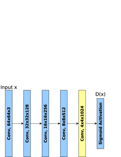
We extract vector representations from the last layer of the discriminator $D$ as shown in Figure 2, and the generator $G$ is trained using the following loss $\mathcal{L}_{G}$ based on the manifold-matching concept:

$$\mathcal{L}_{G} =\|\mathbf{c_{M_{\mathcal{Y}}}}-\mathbf{c_{M_{\mathcal{X}}}}\|_{2}+|\mathbf{\ell_{M_{\mathcal{Y}}}}-\mathbf{\ell_{M_{\mathcal{X}}}}|,$$ (5)

where $M_{\mathcal{Y}}$ is a sphere manifold representing real samples, and $M_{\mathcal{X}}$ is a sphere manifold of generated samples.

In this loss $\mathcal{L}_{G}$, any space mapping is not used. In the next section, we will describe the loss $\mathcal{L}_{G}^{\mathfrak{K}}$ when a space mapping is used. The above loss function requires that the two centroids be the same and that the difference between their radii be zero, which corresponds to the manifold-matching condition in Definition 1.

The discriminator $D$ is trained using the following loss:

$$\mathcal{L}_{D} =\mathcal{L}_{orig}-\mathcal{L}_{G},$$ (6)

where $\mathcal{L}_{orig}$ is the original GAN loss shown in Equation 1 and $-\mathcal{L}_{G}$ is the adversarial version of the generator loss. In other words, the proposed MMGAN performs an adversarial game for manifold-matching.

The training of $D$ is also crucial since we extract vector representations from it. As the discriminator $D$ gets improved, the vector representations also become more accurate. As a result, the training process of MMGAN becomes more reliable. For this reason, we prefer a strong discriminator that is able to produce accurate vector representations to distinguish real and generated images. Recall that the generator is not well trained if the discriminator is too strong in the original GAN [2]. However, our MMGAN is free from the critical problem. This is one of our main contributions in this paper.

IV Reproducing Kernel Hilbert Space (RKHS)

$$\|\varphi(\mathbf{c})-\varphi(\mathbf{s_{i}})\|^{2}_{2} =\mathfrak{K}(\mathbf{c},\mathbf{c})-2\mathfrak{K}(\mathbf{c},\mathbf{s_{i}})+\mathfrak{K}(\mathbf{s_{i}},\mathbf{s_{i}})=\ell_{\mathfrak{K}},$$ (7)

$$\ell_{\mathfrak{K}}=\frac{\sum_{s_{i}\in\mathcal{S}}\|\varphi(\mathbf{c})-\varphi(\mathbf{s_{i}})\|_{2}^{2}}{n} =\frac{\sum_{s_{i}\in\mathcal{S}}\mathfrak{K}(\mathbf{c},\mathbf{c})-2\mathfrak{K}(\mathbf{c},\mathbf{s_{i}})+\mathfrak{K}(\mathbf{s_{i}},\mathbf{s_{i}})}{n},$$

where $\varphi$ is a mapping from the original space to the Hilbert space and $\mathfrak{K}$ is a kernel induced by the mapping $\varphi$. Thus, $\ell_{\mathfrak{K}}$ stands for the radius after the space mapping.

$$\mathcal{L}_{G}^{\mathfrak{K}} =\|\varphi(\mathbf{c_{\mathcal{Y}}})-\varphi(\mathbf{c_{\mathcal{X}}})\|^{2}_{2}+\alpha\cdot\absolutevalue{\ell_{\mathfrak{K},M_{\mathcal{Y}}}-\ell_{\mathfrak{K},M_{\mathcal{X}}}}$$ (8)

$$=\mathfrak{K}(\mathbf{c_{\mathcal{Y}}},\mathbf{c_{\mathcal{Y}}})-2\mathfrak{K}(\mathbf{c_{\mathcal{Y}}},\mathbf{c_{\mathcal{X}}})+\mathfrak{K}(\mathbf{c_{\mathcal{X}}},\mathbf{c_{\mathcal{X}}})$$

$$+\alpha\cdot\absolutevalue{\frac{\sum_{y_{i}\in\mathcal{Y}}\mathfrak{K}(\mathbf{c_{\mathcal{Y}}},\mathbf{c_{\mathcal{Y}}})-2\mathfrak{K}(\mathbf{c_{\mathcal{Y}}},\mathbf{y_{i}})+\mathfrak{K}(\mathbf{y_{i}},\mathbf{y_{i}})}{n}-\frac{\sum_{x_{i}\in\mathcal{X}}\mathfrak{K}(\mathbf{c_{\mathcal{X}}},\mathbf{c_{\mathcal{X}}})-2\mathfrak{K}(\mathbf{c_{\mathcal{X}}},\mathbf{x_{i}})+\mathfrak{K}(\mathbf{x_{i}},\mathbf{x_{i}})}{n}},$$

where $\ell_{\mathfrak{K},M_{\mathcal{X}}}$ and $\ell_{\mathfrak{K},M_{\mathcal{Y}}}$ can be calculated with Equation (7).

Reproducing Kernel Hilbert Space (RKHS) is known to be a flexible approach to represent manifolds. In RKHS, a kernel $\mathfrak{K}$ is used to lay the proposed sphere manifold representing a set $\mathcal{S}=\{\mathbf{s_{1}},\mathbf{s_{2}},\cdots,\mathbf{s_{n}}\}$ in a Hilbert space as Equation (7).

There exist many different kernels, such as linear, Gaussian, and polynomial. In particular, the linear kernel is defined as $\mathfrak{K}(\mathbf{a},\mathbf{b})=\mathbf{a}^{\intercal}\mathbf{b}$, and it reduces to mapping to the original space (i.e., $\varphi(s)=s$ with the linear kernel).

After applying the kernel trick, the loss function to train the generator can be rewritten as $\mathcal{L}_{G}^{\mathfrak{K}}$ in Equation (8). With this kernel trick, we can easily apply various kernels without any explicit space mapping. We skip the description about each kernel function since they are already well-known.

V Correlation Regularization

One key factor of successful training in MMGAN is the diversity of generated samples — more precisely, the diversity in vector representations of generated samples. In an epoch, if all generated samples are similar to each other, then its manifold will be small and all the samples’ vector representations will gather around its centroid, also known as mode collapsing, whereas randomly selected training image samples are usually much more diverse than the generated ones. Even when mode collapsing occurs, two centroids can be similar (i.e., $\|\varphi(\mathbf{c_{\mathcal{Y}}})-\varphi(\mathbf{c_{\mathcal{X}}})\|^{2}_{2}\approx 0$), which is not preferred.

To improve the training procedure, we use the following regularization that promotes the diversity in generated samples at the stage of training the generator $G$. Given a discriminator $D$, the generator is trained so that it can generate more diverse samples.

That is, given a set of vector representations of samples (e.g., $\mathcal{S}=\{\mathbf{s_{1}},\mathbf{s_{2}},\cdots,\mathbf{s_{n}}\}$), we first calculate their $n\times n$ correlation matrix (i.e., normalized covariance matrix) $A_{\mathcal{S}}$. An element $a_{i,j}$ of $A_{\mathcal{S}}$ is a correlation value of vector representations between the $i$-th and the $j$-th samples of $\mathcal{S}$. Then, our proposed regularization term is defined as

$$\mathcal{R}_{G}=\|A-A_{\mathcal{S}}\|_{\mathcal{F}},$$ (9)

where $A$ is an identity matrix, which is the desired correlation matrix and means vector representations are independent from each other; and $\|\cdot\|_{\mathcal{F}}$ is the Frobenius matrix norm. The identity correlation matrix $A$ represents the case that each sample’s vector representation is completely independent and the samples in $\mathcal{S}$ are diverse.

Theorem 1.

If $A_{\mathcal{S}}=A$ in Equation (9), then samples in $\mathcal{S}$ are all different.

Proof.

First, assume that i) no different images have the exactly same vector representation and ii) similar images have similar vector representations. These two assumptions are most likely to be the case if the discriminator is enough trained. In fact, the second assumption is a property of DCGAN.

If mode collapse happens, similar samples will be generated regardless of the input vector $z$, i.e. $G(z_{1})\approx G(z_{2})$, where $z_{1}\neq z_{2}$. Thus, their vector representations will show high correlation (by the second assumption). In other words, $a_{i,j}$ of $A_{S}$, where $i\neq j$, will be close to 1. In the optimal form of the correlation matrix $A$, $a_{i,j}=0$, which means $G(z_{i})\neq G(z_{j})$ (i.e., no mode collapse).

Therefore, if $\mathcal{R}_{G}=0$, then there is no mode-collapse. ∎

Finally, in MMGAN, neural networks are trained with the following loss functions:

$$\begin{split}\mathcal{L}_{G}^{final}&=\begin{cases}\mathcal{L}_{G}+\beta\cdot\mathcal{R}_{G},&\textrm{without any kernel}\\ \mathcal{L}_{G}^{\mathfrak{K}}+\beta\cdot\mathcal{R}_{G},&\textrm{with a kernel $\mathfrak{K}$}\end{cases}\\ \mathcal{L}_{D}^{final}&=\mathcal{L}_{orig}-\mathcal{L}_{G}^{final}\end{split}$$ (10)

where $\alpha$ and $\beta$ are weight parameters and $\mathcal{L}_{G}$ and $\mathcal{L}_{G}^{\mathfrak{K}}$ are defined in Equations (6) and (8), respectively.

VI Training Algorithm

Algorithm 1 describes the training procedures of MMGAN based on the proposed loss functions. Basically, the overall training procedure is the same as the original GAN, but the main difference is that we maintain two manifolds representing $p_{data}$ and $p_{g}$ by using the exponentially-weighted moving average calculation of $\mathbf{c_{\mathcal{Y}}}$, $\mathbf{\boldsymbol{\ell}_{\mathcal{Y}}}$, $\mathbf{c_{\mathcal{X}}}$, and $\mathbf{\boldsymbol{\ell}_{\mathcal{X}}}$. With this moving average calculation, we aim to find statistically meaningful manifolds because we consider all the previous samples. In particular, we set $\delta$ as $0.9$ or greater so that we can give a large weight on the cumulative manifold information rather than the manifold representing only the mini-batch samples.

 Input: real samples: $\{x_{1},x_{2},\cdots\}\sim p(x)$

Output: a generative model $G$

1  $G\leftarrow$ a generative neural network

2 $D\leftarrow$ a discriminator neural network

3 while until convergence do

4       Create a mini-batch of real samples $Y_{mini}=\{y_{1},\cdots,y_{n}\}$

5       Create a set of generated samples $Z_{mini}=\{z_{1},\cdots,z_{n}\}$ and their generated images $X_{mini}=\{G(z_{0}),\cdots,G(z_{n})\}$

6       Train the discriminator $D$ with $\mathcal{L}_{D}^{final}$

       /* Moving average update of the centroid and the radius for $p_{data}$ */

7       $\mathbf{c_{\mathcal{Y}}}=\delta\times\mathbf{c_{\mathcal{Y}}}+(1-\delta)\times\mathbf{c_{\mathcal{Y}_{mini}}}$

8       $\mathbf{\boldsymbol{\ell}_{\mathcal{Y}}}=\delta\times\mathbf{\boldsymbol{\ell}_{\mathcal{Y}}}+(1-\delta)\times\mathbf{\boldsymbol{\ell}_{\mathcal{Y}_{mini}}}$

       /* Moving average update of the centroid and radius for $p_{g}$ */

9       $\mathbf{c_{\mathcal{X}}}=\delta\times\mathbf{c_{\mathcal{X}}}+(1-\delta)\times\mathbf{c_{\mathcal{X}_{mini}}}$

10       $\mathbf{\boldsymbol{\ell}_{\mathcal{X}}}=\delta\times\mathbf{\boldsymbol{\ell}_{\mathcal{X}}}+(1-\delta)\times\mathbf{\boldsymbol{\ell}_{\mathcal{X}_{mini}}}$

11       Train the generator $G$ with $\mathcal{L}_{G}^{final}$

12      

13 end while

14return $G$

 

Algorithm 1 Training algorithm of MMGANs. $\mathcal{Y}_{mini}$ (resp. $\mathcal{X}_{mini}$) is the set of vector representations of a set of real samples $Y_{mini}$ (resp. generated samples $X_{mini}$)

The runtime of Algorithm 1 remains similar to it of IGAN except the correlation regularization that additionally incurs a couple of $n\times d$ matrix multiplications. However, this is not significant because existing deep learning platforms can quickly calculate.

VII Experiments

In this section, we describe our evaluation environments and results. The source code and datasets of all the experiments used in this paper will be available at (github.com/npark/MMGAN) upon publication. Now we are cleaning them. We forked the DCGAN and IGAN source codes and implemented our MMGAN on our own.

Note that there exists no solid metric to quantitatively evaluate the quality of generated images. While the inception score [20] can be used for some images, we generally rely on humans’ visual perception to evaluate the quality of generated samples.

VII-A Experimental Setup

We use three image datasets, MNIST [13], CelebA [14], and CIFAR-10 [12]. The MNIST database, one of the most popular evaluation datasets, contains 60,000 hand-written digit images. CelebA has over 360,000 celebrity face images with a large variety of facial poses. CIFAR-10 consists of 52,000 images from 10 different object classes. While the images in CelebA and CIFAR-10 have RGB channels, MNIST images are grey-scale ones.

We rely on human visual perception to evaluate MNIST and CelebA since there is no quantitative evaluation metric. To this end, we created a website for a user study, where given randomly chosen images, participants are asked to distinguish between real and fake images. More than 30 people from three different continents participated in the study. Each participant performed the same number of trials for each generative method to avoid any potential biases. We demonstrate how many fake images are correctly identified as fake for each method.

For CIFAR-10, we primarily use the inception score defined in [20]. It uses the inception model [21] to detect objects in generated images. The inception score is designed to give high scores if various and high-quality objects are recognized in the generated samples.

We used a cluster of machines running Linux with Xeon CPU, 32GB RAM, and K80 GPUs for all our experiments, and the Tensorflow [1] and Theano [6] deep neural network libraries.

VII-B Experimental Results

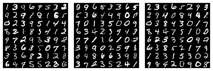
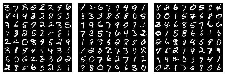
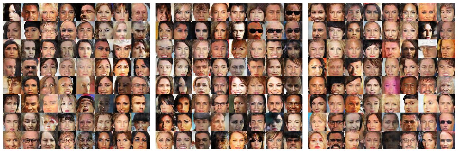
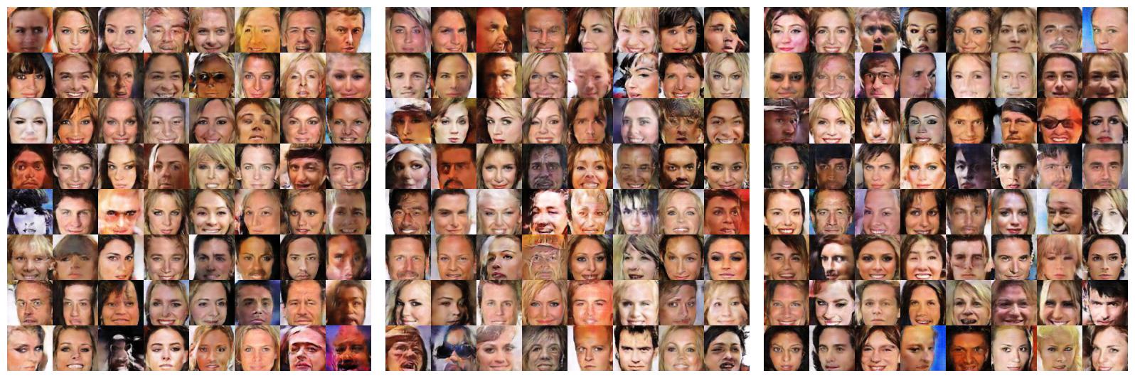
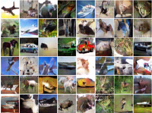
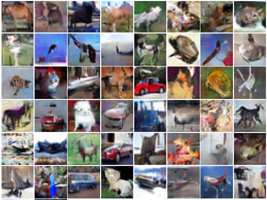
In Figure 3, we show generation examples for some random mini-batches at the last epoch. We did not cherry-pick them. It is very noticeable that almost all images are visually recongnizable.

TABLE I: The percentage of samples selected as fake in the user study. Lower values are preferred.

Dataset	Real	DCGAN	MMGAN on DCGAN (RBF Kernel)	MMGAN on DCGAN (EXP Kernel)	MMGAN on DCGAN (No $\mathcal{R}_{G}$)
MNIST	14%	38.2%	32.4%	35.4%	45.5%
CelebA	4%	75.3%	77%	73.3%	76.6%

(a) DCGAN

(b) MMGAN (RBF, $\alpha=1.0$, $\beta=1.0$)

(c) DCGAN

(d) MMGAN (EXP, $\alpha=1.0$, $\beta=1.0$)

(e) MMGAN (RBF, $\alpha=1.0$, $\beta=0.1$)

(f) MMGAN (EXP, $\alpha=1.0$, $\beta=0.1$)

GAN model	DCGAN	MMGAN on DCGAN (RBF Kernel)	AGE
Inception score	6.8	$6.96\pm 0.06$	5.6
GAN model	IGAN	MMGAN on IGAN (EXP Kernel)	$\alpha$-GAN
Inception score	6.86 $\pm$ 0.06	7.8 $\pm$ 0.06	7.0

(g) Inception score for CIFAR-10 (class-unsupervised training)

Figure 3: Generated samples for (a)-(b) MNIST, (c)-(d) CelebA, (e)-(f) CIFAR-10, and (g) inception score for CIFAR-10. We did not cherry-pick generated images but show random mini-batches. Note that almost all generated images show high quality.

VII-B1 MNIST

Figure 3 (a) and (b) shows those image samples generated by DCGAN and MMGAN (implemented after modifying DCGAN). Figure 3(a) are generated examples available at the official github repository of DCGAN. Many samples are properly recognizable by humans, while a few samples are of poor quality. Figures 3(b) shows images generated by MMGAN with the RBK kernel.

Our user study results in Table I show that MMGAN received a less number of downvotes than DCGAN. This indicates that the participants considered MMGAN-generated images more realistic than DCGAN-generated images. Note also that without the correlation regularization, MMGAN does not outperform DCGAN, which implies that the proposed manifold-matching becomes more robust when generated samples are diverse.

Interestingly, 14% of real images of MNIST also received downvotes. This means our high-quality generated images make participants confused and they committed non-trivial mistakes in the user study.

VII-B2 CelebA

Figure 3 (c) and (d) show the comparison of CelebA samples generated by DCGAN and MMGAN (implemented after modifying DCGAN). The user study results show that many images generated by DCGAN and MMGAN were commonly identified as fake by participants. However, MMGAN slightly outperforms DCGAN. It is more challenging to generate high-quality images for CelebA than MNIST and CIFAR-10 because CelebA does not have labels and all facial images look similar whereas MNIST and CIFAR-10 contain diverse hard-written digits and objects.

VII-B3 CIFAR-10

For CIFAR-10, we compare $\alpha$-GAN [18], DCGAN, IGAN,and MMGAN (implemented after modifying both DCGAN and IGAN). IGAN is the state-of-the-art method for this dataset [8]. We use the inception score (rather than visual evaluations). $\alpha$-GAN is based on auto-encoders. $\alpha$-GAN was very recently released and outperforms other auto-encoder-based models such as [22] by a considerable margin.

Note that MMGAN performs better than DCGAN and IGAN, as shown in the table of Figure 3 (g). This highlights the superiority of MMGAN in comparison with conventional GAN training procedures. IGAN reported the inception score of 6.86 and our MMGAN on top of it marked a much better score. Samples generated by MMGAN is in Figure 3 (e) and (f).

VIII Conclusion

In this paper, we proposed a novel GAN model based on manifold-matching (MMGAN). The proposed MMGAN differs from other existing GAN models, especially with respect to the training loss function of the generator. Instead of the predictions $D(x)$ and $D(G(z))$ made by the discriminator, MMGAN extracts vector representations of real and fake images from the last layer of the discriminator and calculate an approximated manifold for each of the set of real images and that of fake ones. In order to better train the generator, MMGAN requires that the two manifolds (corresponding to the real and generated data) match. MMGANs hence benefit from a more accurate discriminator, which enables them to make more accurate vector representations of images. Our experiments demonstrates that MMGAN shows comparable or better performance in comparison with other popular GAN models for three image datasets.

References

- [1] M. Abadi, A. Agarwal, P. Barham, E. Brevdo, Z. Chen, C. Citro, G. S. Corrado, A. Davis, J. Dean, M. Devin, et al. Tensorflow: Large-scale machine learning on heterogeneous distributed systems. arXiv preprint arXiv:1603.04467, 2016.
- [2] M. Arjovsky and L. Bottou. Towards principled methods for training generative adversarial networks. CoRR, abs/1701.04862, 2017.
- [3] M. Arjovsky, S. Chintala, and L. Bottou. Wasserstein gan. arXiv preprint arXiv:1701.07875, 2017.
- [4] J. Bao, D. Chen, F. Wen, H. Li, and G. Hua. CVAE-GAN: fine-grained image generation through asymmetric training. CoRR, abs/1703.10155, 2017.
- [5] M. G. Bellemare, I. Danihelka, W. Dabney, S. Mohamed, B. Lakshminarayanan, S. Hoyer, and R. Munos. The cramer distance as a solution to biased wasserstein gradients. CoRR, abs/1705.10743, 2017.
- [6] J. Bergstra, O. Breuleux, P. Lamblin, R. Pascanu, O. Delalleau, G. Desjardins, I. Goodfellow, A. Bergeron, Y. Bengio, and P. Kaelbling. Theano: Deep learning on gpus with python. 2011.
- [7] I. Goodfellow, J. Pouget-Abadie, M. Mirza, B. Xu, D. Warde-Farley, S. Ozair, A. Courville, and Y. Bengio. Generative adversarial nets. In Advances in neural information processing systems, pages 2672–2680, 2014.
- [8] I. J. Goodfellow. NIPS 2016 tutorial: Generative adversarial networks. CoRR, abs/1701.00160, 2017.
- [9] R. D. Hjelm, A. P. Jacob, T. Che, K. Cho, and Y. Bengio. Boundary-seeking generative adversarial networks. arXiv preprint arXiv:1702.08431, 2017.
- [10] T. Hofmann, B. Schölkopf, and A. J. Smola. Kernel methods in machine learning. Annals of Statistics, 36(3):1171–1220, 2008.
- [11] T. Kim and Y. Bengio. Deep Directed Generative Models with Energy-Based Probability Estimation. ArXiv e-prints, June 2016.
- [12] A. Krizhevsky, V. Nair, and G. Hinton. Cifar-10 (canadian institute for advanced research).
- [13] Y. LeCun and C. Cortes. MNIST handwritten digit database. 2010.
- [14] Z. Liu, P. Luo, X. Wang, and X. Tang. Deep learning face attributes in the wild. In Proceedings of International Conference on Computer Vision (ICCV), 2015.
- [15] Y. Mroueh, T. Sercu, and V. Goel. Mcgan: Mean and covariance feature matching GAN. CoRR, abs/1702.08398, 2017.
- [16] H. Narayanan and S. Mitter. Sample complexity of testing the manifold hypothesis. In J. D. Lafferty, C. K. I. Williams, J. Shawe-Taylor, R. S. Zemel, and A. Culotta, editors, Advances in Neural Information Processing Systems 23, pages 1786–1794. Curran Associates, Inc., 2010.
- [17] A. Radford, L. Metz, and S. Chintala. Unsupervised representation learning with deep convolutional generative adversarial networks. arXiv preprint arXiv:1511.06434, 2015.
- [18] M. Rosca, B. Lakshminarayanan, D. Warde-Farley, and S. Mohamed. Variational Approaches for Auto-Encoding Generative Adversarial Networks. ArXiv e-prints, June 2017.
- [19] S. T. Roweis and L. K. Saul. Nonlinear dimensionality reduction by locally linear embedding. SCIENCE, 290:2323–2326, 2000.
- [20] T. Salimans, I. J. Goodfellow, W. Zaremba, V. Cheung, A. Radford, and X. Chen. Improved techniques for training gans. CoRR, abs/1606.03498, 2016.
- [21] C. Szegedy, V. Vanhoucke, S. Ioffe, J. Shlens, and Z. Wojna. Rethinking the inception architecture for computer vision. CoRR, abs/1512.00567, 2015.
- [22] D. Ulyanov, A. Vedaldi, and V. S. Lempitsky. Adversarial generator-encoder networks. CoRR, abs/1704.02304, 2017.
- [23] J. Zhao, M. Mathieu, and Y. LeCun. Energy-based Generative Adversarial Network. ArXiv e-prints, Sept. 2016.