Cross-Correlation Redshift Calibration Without Spectroscopic Calibration Samples in DES Science Verification Data

Abstract

Galaxy cross-correlations with high-fidelity redshift samples hold the potential to precisely calibrate systematic photometric redshift uncertainties arising from the unavailability of complete and representative training and validation samples of galaxies. However, application of this technique in the Dark Energy Survey (DES) is hampered by the relatively low number density, small area, and modest redshift overlap between photometric and spectroscopic samples. We propose instead using photometric catalogs with reliable photometric redshifts for photo-$z$ calibration via cross-correlations. We verify the viability of our proposal using redMaPPer clusters from the Sloan Digital Sky Survey (SDSS) to successfully recover the redshift distribution of SDSS spectroscopic galaxies. We demonstrate how to combine photo-$z$ with cross-correlation data to calibrate photometric redshift biases while marginalizing over possible clustering bias evolution in either the calibration or unknown photometric samples. We apply our method to DES Science Verification (DES SV) data in order to constrain the photometric redshift distribution of a galaxy sample selected for weak lensing studies, constraining the mean of the tomographic redshift distributions to a statistical uncertainty of $\Delta z\sim\pm 0.01$. We forecast that our proposal can in principle control photometric redshift uncertainties in DES weak lensing experiments at a level near the intrinsic statistical noise of the experiment over the range of redshifts where redMaPPer clusters are available. Our results provide strong motivation to launch a program to fully characterize the systematic errors from bias evolution and photo-$z$ shapes in our calibration procedure.

1 Introduction

The determination of the photometric redshift distribution of a given source population is fraught with difficulties. For instance, the two primary methods for determining the redshift distribution of photometric objects — template fitting and machine learning — must both confront a critical difficulty: the spectroscopy available for training, calibration, and validation of photometric redshift techniques is rarely representative of the magnitude and color-space distribution of all survey galaxies. It is possible to mitigate this problem by weighting spectroscopic galaxies such that they better represent the photometric properties of the whole photometric survey (Lima et al., 2008; Cunha et al., 2009; Sánchez et al., 2014; Bonnett et al., 2016, Hoyle et al. in prep.). However, for this method to be effective, the training set must be complete relative to the photometric data, such that it densely covers and spans the same space of relevant photometric observables as the full survey. This is difficult to achieve in regions that lack spectroscopic data, particularly at high redshifts. Similarly, available templates may not span the full color-redshift-space (Bonnett et al., 2016) of the galaxies of interest. This problem tends to be particularly acute for the faint galaxies which make up the majority of the sources used for weak gravitational lensing. In order to precisely and accurately determine the dark energy equation of state from photometric weak lensing and large-scale structure measurements, it is vital to precisely characterize the redshift distributions of the tomographic redshift bins into which the galaxies are split. Bonnett et al. (2016) find that photometric redshifts biases must be controlled at the $\sim\!0.003$ level in order for the Dark Energy Survey (DES) 5,000 $\deg^{2}$ survey to not be limited by photometric redshift uncertainties. While ‘photo-$z$’ methods have made considerable progress towards meeting these requirements, current performance falls short of this goal. As such, any method with the potential to further improve this calibration is of great interest as a possible way to reduce, and perhaps even eliminate, the photo-$z$ systematics floor of photometric surveys like the DES.

Newman (2008) was the first to demonstrate that by cross-correlating a sample of photometric galaxies with unknown redshift distribution with thin redshift slices of a spectroscopic galaxy sample one could recover the redshift distribution of the photometric galaxy sample. This method was improved by Matthews & Newman (2010) using an iterative technique to account for the evolution in galaxy clustering bias. Several others have tested the method on N-body simulations with promising results, including various methods for further improving and refining the cross-correlation method (Schulz, 2010; Matthews & Newman, 2012; Schmidt et al., 2013; McQuinn & White, 2013; McLeod et al., 2016; Scottez et al., 2017; van Daalen & White, 2017). The method has also been applied to data: Benjamin et al. (2010) used cross-correlations to measure the degree of artificial contamination in tomographic redshift bins and applied the technique to the Canada-France-Hawaii Telescope Legacy Survey (CFHTLS), and Ménard et al. (2013) used clustering measurements on both linear and modestly non-linear scales to characterize the redshift distributions of SDSS, WISE, and FIRST galaxies.

More recently, Rahman et al. (2015) combined clustering information with photometry to show how the cross-correlation method can recover the redshift probability distribution of an individual galaxy. Schmidt et al. (2015) cross-correlated Planck High Frequency Instrument maps against SDSS quasars to estimate the distribution of the cosmic infrared background. Rahman et al. (2016) mapped the relation between galaxy color and redshift by using cross-correlations instead of spectral energy distribution templates, and Scottez et al. (2016) apply the same estimations to VIPERS. Sun et al. (2015) extend cross-correlations to the Fourier domain by examining how galaxy angular power spectra can determine the mean redshift to percent precision. Lee et al. (2016) use integer linear programming to optimize cross- and autocorrelations, demonstrating that it is possible to assign individual galaxies to redshift bins via clustering signals alone. Choi et al. (2016) used cross-correlations to check the validity of using summed $p(z)$ to determine galaxy redshift distributions in both CFHTLS and the Red-sequence Cluster Lensing Survey.

Most recently, Hildebrandt et al. (2017) used cross-correlation methods to validate the photometric redshift distribution of source galaxies in the Kilo Degree Survey (KiDS) via the open source code The-wiZZ described in Morrison et al. (2017). Johnson et al. (2017) extended the quadratic estimator from McQuinn & White (2013) and found qualitative agreement with the results from Hildebrandt et al. (2017). Importantly, those efforts were hampered by the low number of spectroscopic galaxies available for photo-$z$ calibration via cross-correlations across a broad redshift range. This relative lack of spectroscopic calibration samples for cross-correlation studies is a serious obstacle to the realization of the promise that these methods hold.

One solution to the relative paucity of spectroscopic galaxies in the footprint of these wide-field optical photometric surveys is to use other objects which have reasonably precise redshifts but which are far more numerous. One example for such a class of objects are redMaPPer galaxy clusters described in Rykoff et al. (2014), who present a red sequence cluster finder that produces objects with nearly Gaussian estimated redshifts and scatter $\sigma_{z}/(1+z)\sim 0.01$. The method relies on a small set of spectroscopic objects for training, but can then be used to find objects over the full survey footprint to much fainter magnitudes. Importantly, while these objects are rare, the complete overlap between these photometrically selected objects and the galaxies that are to be calibrated means that the cross-correlation signal can be measured with high signal-to-noise. This makes them a natural candidate for calibrating redshift distributions in photometric wide-field surveys. Note, however, that such cross-correlation measurements are by necessity limited to the redshift range over which the red sequence is well calibrated.

In this paper we examine how well the cross-correlation method performs when, instead of spectroscopic galaxies, objects with accurate photometric redshifts are used as the reference sample. We wish to examine the following questions:

• How well do cross-correlation methods with non-spectroscopic reference samples perform in comparison with spectroscopic reference samples?

• How can we properly combine photo-$z$ and cross-correlation information to minimize the noise inherent to cross-correlation methods while reducing the redshift biases from standard photo-$z$ methods?

• How does using non-spectroscopic reference samples to constrain the redshift distributions of galaxies impact cosmological parameter estimation?

This paper is organized as follows. In Section 2 we present the datasets used in this study. In Section 3 we review the theory behind the cross-correlation method and present our method for calculating redshift distributions from cross-correlations. In Section 4 we present the performance of cross-correlations when using redMaPPer clusters as reference objects, and compare our results to those obtained when using SDSS spectroscopic galaxies as reference. We also examine the impact of using different weighting functions and integration ranges on the accuracy and precision of the recovered redshift distributions. In Section 5 we apply our method to the Dark Energy Survey Science Verification dataset, and examine how we can use the cross-correlation method to determine the redshift bias in photometric redshift methods. In Section 6 we forecast the performance of using the cross-correlation method to constrain cosmological parameters with the Dark Energy Survey Year Five data. We wrap up in Section 7 and discuss potential future applications of this method.

Throughout this paper we assume a WMAP9 cosmology ($\Omega_{m}=0.286$) and report distances in $h^{-1}$ Mpc. We find that the choice of cosmology has a negligible impact on our results (Hinshaw et al., 2013).

2 Datasets

Our analysis relies on four catalogs drawn from two galaxy surveys, the Sloan Digital Sky Survey (SDSS) and the Dark Energy Survey Science Verification (DES SV). Each of these data sets and the corresponding catalogs are detailed below.

2.1 SDSS Spectroscopic Galaxy Samples

The SDSS spectroscopic galaxy sample consists of the LOWZ and CMASS galaxy samples from the Baryon Oscillation Spectroscopic Survey (BOSS) (Alam et al., 2015). BOSS obtained data over 9376 deg² divided into two regions in the Northern and Southern Galactic Caps. The LOWZ sample is a set of galaxies uniformly targeted for large-scale structure studies in a relatively low redshift range ($z<0.43$). The CMASS sample is a set of galaxies over the range ($0.43<z<0.7$) designed to create an approximately volume-limited sample in stellar mass. Both catalogs come with ‘randoms,’ catalogs that reflect the footprints and selection functions of the two surveys. For our purposes here it is sufficient to simply combine the two catalogs over their full redshift ranges, which we shall collectively refer to as the SDSS catalog.

2.2 redMaPPer

redMaPPer is a red sequence cluster finder originally developed within the context of the SDSS (Rykoff et al., 2014; Rozo et al., 2015b). The red sequence is the empirical relation that early-type galaxies in rich clusters lie along a linear color-magnitude relation with small scatter (Bower et al., 1992; Bell et al., 2004). redMaPPer iteratively self-trains a model of the red sequence based on sparse spectroscopic data, and then uses this model to identify clusters of red sequence galaxies, and to estimate the photometric redshift of the resulting clusters. The algorithm has been extensively tested and validated (Rozo et al., 2015a). In addition to the SDSS catalog, we use the redMaPPer cluster catalog resulting from the application of the redMaPPer algorithm to the DES SV data (Rykoff et al., 2016). While the redMaPPer cluster catalog from SDSS is therefore different from the one used in DES SV, in that the algorithm has been applied to a different set of galaxies, the number density and the mass-richness relations are similar, and most importantly, the performance in photo-$z$ is the same. These catalogs come with their own associated ‘randoms’ which reflect the footprint and the ability to select a redMaPPer cluster of some richness $\lambda$ at a given location. We have chosen clusters with $\lambda>5$. For our purposes, the most important aspect of the redMaPPer cluster catalog is its exquisite redshift performance: cluster photo-$z$’s are both accurate (photo-$z$ redshift biases are at the $0.005$ level or less) and precise (photo-$z$ scatter is $\sigma_{z}/(1+z)\sim 0.01$) with a $4\sigma$ outlier fraction of at most 3%. As such, the redMaPPer clusters are excellent candidates for photometric reference samples when attempting to perform photo-$z$ calibration via cross-correlation.

Unfortunately, the redMaPPer clusters do not span the full redshift range of the samples we consider in this paper. In SDSS, the redshift range of the redMaPPer clusters used is $0.1<z<0.56$, while in DES SV we take advantage of the greater depth and look at clusters in the range $0.2<z<0.85$. The greater redshift reach in the DES SV region is due to the greater depth of the photometric data. In contrast, the SDSS spectroscopic galaxies extend to $z<0.7$, while the source galaxies in DES SV can have redshifts of $z>1$.

2.3 DES SV

The Dark Energy Survey is an ongoing $5000\ \mathrm{deg}^{2}$ photometric survey in the $grizY$ bands performed with the Dark Energy Camera (DECam, Flaugher et al., 2015). Before the beginning of the survey, the DES conducted a $\sim 250\,\mathrm{deg}^{2}$ “Science Verification” (SV) survey. The main portion of the SV footprint, used in this paper, covers $139\ \mathrm{deg}^{2}$ in the range $65<\mathrm{R.A.}<93$ and $-60<\mathrm{Decl.}<-42$. The region is dubbed South Pole Telescope East (SPTE) because of its location and overlap with the South Pole Telescope survey area (SPT, Carlstrom et al., 2011). SPTE was observed with 2-10 tilings in each of the $griz$ filters. In addition, the DES observes 10 Supernova fields every 5-7 days, each of which covers a single DECam 2.2 degree-wide field-of-view. The median depth of the SV survey (defined as $10\sigma$ detections for extended sources) are $g=24.0$, $r=23.8$ $i=23.0$, $z=22.3$, and $Y=20.8$.

The DES SV data were processed by the DES Data Management (DESDM) infrastructure (Morganson et al, in prep, see also Sevilla et al., 2011; Desai et al., 2012). We used SExtractor (Bertin & Arnouts, 1996; Bertin, 2011) to detect photometric sources based on a “chi-squared” coadd of $r$, $i$, and $z$ images obtained with SWarp (Bertin, 2010). The catalog was then further refined to produce the DES “SVA1 Gold” catalog. Galaxy magnitudes and colors are computed via the SExtractor MAG_AUTO quantity. This SVA1 Gold catalog is the fundamental input to the construction of the DES SV NGMIX galaxy sample and the DES SV redMaPPer cluster catalog.

2.4 NGMIX

From the SVA1 Gold catalog, we examine a subsample of galaxies used for cosmic shear measurements. The NGMIX pipeline (Sheldon, 2014) estimates the shapes of the galaxies in the SVA1 catalog. The subsample is then selected by cutting objects with very low surface brightnesses and small sizes, and choosing only objects with reasonable colors ($-1<g-r<4$ and $-1<i-z<4$). NGMIX represents galaxies as sums of Gaussians (Hogg & Lang, 2013). The same model shape is fitted simultaneously across multiple exposures in the riz bands using Markov Chain Monte Carlo techniques applied to a full likelihood which forward models the galaxy by convolving with the exposure PSF. The final effective source number density of the NGMIX catalog is $\sim 6.1$ galaxies per square arcminute (Becker et al., 2016). The shape systematics in the NGMIX catalog are tangential to this paper to the extent that they do not imprint a spatial correlation on the footprint. However, interested readers should look to Jarvis et al. (2016) for a thorough examination of shape systematics.

Galaxy photo-$z$’s for the NGMIX catalog are estimated using four different photometric redshift algorithms: the template-based algorithm BPZ (Benítez, 1999; Coe et al., 2006), and the machine learning algorithms SkyNet (Graff et al., 2014; Bonnett, 2015), TPZ (Carrasco Kind & Brunner, 2013, 2014), and ANNZ2 (Sadeh et al., 2016). Extensive testing of the algorithms was carried out in Sánchez et al. (2014) and Bonnett et al. (2016), to which we refer the reader for further detail on the algorithms. We do not include the calibration offset to BPZ that was measured in Bonnett et al. (2016). For our purposes, the key point is that each of these algorithms return a redshift probability distribution $P(z)$ for each galaxy, the sum of which can be used as a (biased) estimator for the redshift distribution of the galaxies under consideration (Asorey et al., 2016).

3 Theory and Methods

We outline the theory in this section and present our estimator. The approach presented here is based on Ménard et al. (2013). We repeat much of the argument here, though the focus and presentation are somewhat different. Our goal is not to be repetitious, but to simply present an alternative but fully equivalent discussion.

Let $\rho$ be the comoving galaxy density. In a flat universe, the corresponding galaxy density per unit angular area per unit redshift $d^{2}N/d\Omega dz$ is given by

$$\frac{d^{2}N}{d\Omega dz}(d\Omega dz)=\rho(z)\chi^{2}(z)\frac{d\chi}{dz}d\Omega dz=\rho(z)\chi^{2}(z)cH^{-1}(z)d\Omega dz.$$ (1)

where $\chi$ is the comoving distance and $H$ is the Hubble parameter. One has then

$$\nu\equiv\frac{d^{2}N}{d\Omega dz}=\bar{\rho}(z)\chi^{2}(z)cH^{-1}(z)\left[1+\delta(\chi(z)\theta,\chi(z))\right]\\$$ (2)

where $\nu$ is the angular galaxy density per unit redshift and per unit angular area, $\delta$ is the fractional matter overdensity relative to the mean density, and $\theta$ is the angular separation.

Let $n(\theta)=dN/d\Omega$ be the projected galaxy density. One has

$$n(\theta)=\int dz\ \bar{\rho}(z)\chi^{2}(z)cH^{-1}(z)\left[1+\delta(\chi(z)\theta,\chi(z))\right].$$ (3)

The mean galaxy density is simply

$$\bar{n}=\int dz\ \bar{\rho}(z)\chi^{2}(z)cH^{-1}(z),$$ (4)

while the redshift distribution of the galaxies $\phi(z)$ is defined such that $\bar{n}\phi(z)$ is the mean galaxy density per unit redshift, i.e.

$$\bar{n}\phi(z)=\bar{\nu}=\bar{\rho}(z)\chi^{2}(z)cH^{-1}(z)$$ (5)

We can therefore write

$$n(\theta)=\bar{n}\int dz\ \phi(z)\left[1+\delta(\chi(z)\theta,\chi(z))\right]$$ (6)

where $\phi(z)$ integrates to unity. Setting $n(\theta)=\bar{n}(1+\Delta)$, we see that

$$\Delta(\theta)=\int dz\ \phi(z)\delta(\chi\theta,\chi).$$ (7)

Consider now two galaxy samples, one of which has known redshifts, which we refer to as the reference sample with subscript ‘ref,’ and one which has an unknown redshift distribution, which we refer to as the unknown sample with subscript ‘u.’ We wish to consider the cross-correlation between the unknown sample and reference galaxies within a narrow redshift bin. The angular cross-correlation between the reference and unknown samples is therefore

$$w(\theta) =\langle\Delta_{\rm{u}}\Delta_{\rm{ref}}\rangle(\theta)$$ (8)

$$=\int dzdz^{\prime}\ \phi_{\rm{u}}(z)\phi_{\rm{ref}}(z^{\prime})b_{\rm{u}}(\theta,z)b_{\rm{ref}}(\theta,z^{\prime})\xi(\chi\theta,\chi;\chi^{\prime}\theta,\chi^{\prime})$$ (9)

where $\xi$ is the matter–matter correlation function $\langle\delta(\chi\theta,\chi)\delta(\chi^{\prime}\theta,\chi^{\prime})\rangle$ and we allow the galaxy clustering bias $b$ to have both redshift and scale dependence for some separation $\theta$ and redshift $z$. Consider the case $\phi_{\rm{ref}}(z)=\delta(z-z_{\rm{ref}})$ where $z_{\rm{ref}}$ is some reference redshift. This is equivalent to selecting a reference sample in an infinitely narrow redshift slice. We have then

$$w(\theta,z_{\rm{ref}})=b_{\rm{ref}}(\theta,z_{\rm{ref}})\int dz\ \phi_{\rm{u}}(z)b_{\rm{u}}(\theta,z)\xi(\chi\theta,\chi;\chi^{\prime}\theta,\chi^{\prime}).$$ (10)

Now, $\xi$ is zero unless $\chi\sim\chi^{\prime}=\chi(z_{\rm{ref}})$. Using a flat sky approximation, and adopting the origin at a reference galaxy when measuring the angular separation we find

$$w(\theta,z_{\rm{ref}})=b_{\rm{ref}}(\theta,z_{\rm{ref}})\int dz\ \phi_{\rm{u}}(z)b_{\rm{u}}(\theta,z)\ \times$$

$$\xi\left(\left[\Delta\chi^{2}(z,z_{\rm{ref}})+\chi(z_{\rm{ref}})^{2}\theta^{2}\right]^{1/2};z_{\rm{ref}}\right)$$ (11)

where $\Delta\chi=\chi(z)-\chi(z_{\rm{ref}})$. We assume $\xi$ varies much more quickly than $\phi_{\rm{u}}$ or $b_{\rm{u}}$. Since $\xi$ is non-zero only over a small redshift range $z\sim z_{\rm{ref}}$, we arrive at

$$w(\theta,z_{\rm{ref}})=\ \phi_{\rm{u}}(z_{\rm{ref}})b_{\rm{u}}(\theta,z_{\rm{ref}})b_{\rm{ref}}(\theta,z_{\rm{ref}})\ \times$$

$$\int dz\ \xi\left(\left[\Delta\chi^{2}+\chi(z_{\rm{ref}})^{2}\theta^{2}\right]^{1/2};z_{\rm{ref}}\right).$$ (12)

It is useful to rephrase the correlation function in terms of the physical transverse separation $r=D_{A}\theta=(1+z)^{-1}\chi\theta$. The integral of the correlation function is simply the projected correlation function for matter,

$$w_{\rm{mm}}(r,z_{\rm{ref}})=\int dz\ \xi\left(\left[(\chi(z)-\chi(z_{\rm{ref}}))^{2}+(1+z)^{2}r^{2}\right]^{1/2};z_{\rm{ref}}\right).$$ (13)

Again, note we have opted to utilize physical units for $r$. Plugging in we arrive at

$$w(r,z_{\rm{ref}})=\phi_{\rm{u}}(z_{\rm{ref}})b_{\rm{u}}(r,z_{\rm{ref}})b_{\rm{ref}}(r,z_{\rm{ref}})w_{\rm{mm}}(r,z_{\rm{ref}}).$$ (14)

If we define the growth $G(r,z_{\rm{ref}})$ relative to some arbitrary redshift $z_{0}$ via

$$w_{\rm{mm}}(r,z_{\rm{ref}})=G(r,z_{\rm{ref}})w_{\rm{mm}}(r,z_{0})$$ (15)

our final expression becomes

$$w(r,z_{\rm{ref}})=\phi_{\rm{u}}(z_{\rm{ref}})b_{\rm{u}}(r,z_{\rm{ref}})b_{\rm{ref}}(r,z_{\rm{ref}})G(r,z_{\rm{ref}})w_{\rm{mm}}(r,z_{0}).$$ (16)

Note $G$ is not necessarily the linear growth factor, and in fact, $G$ can depend on the length scale $r$. We collect $b_{\rm{u}}(r,z_{\rm{ref}})$, $b_{\rm{ref}}(r,z_{\rm{ref}})$, and $G(r,z_{\rm{ref}})$ into a single source function $f(r,z_{\rm{ref}})$ to write:

$$w(r,z_{\rm{ref}})=\phi_{\rm{u}}(z_{\rm{ref}})f(r,z_{\rm{ref}})w_{\rm{mm}}(r)$$ (17)

where we have made the evaluation $z=z_{0}$ of $w_{\rm{mm}}$ implicit. We will address how we handle the function $f(r,z_{\rm{ref}})$ momentarily.

We measure the angular correlation function by counting the number of pairs between our unknown and reference data $\mathrm{D_{u}}\mathrm{D_{r}}$ separated over a range of scales $r_{\rm{min}}$ to $r_{\rm{max}}$ weighted by some function $W(r)$. We take $W(r)$ to be a power-law, $W(r)\propto r^{\alpha}$. We discuss how we select the value $\alpha$ and the radial range $r_{\rm{min}}$ to $r_{\rm{max}}$ in Sections 4 and 5 below.

Given the true angular correlation $w$, the number of unknown–reference pairs is:

$$\mathrm{D_{u}}\mathrm{D_{r}}(z)=n_{\mathrm{u}}n_{\mathrm{r}}A_{\mathrm{survey}}A_{\mathrm{shell}}\int_{r_{\rm{min}}}^{r_{\rm{max}}}dr\ W(r)\left[1+w(r,z)\right]\ ,$$ (18)

where $n_{\mathrm{u}}$ and $n_{\mathrm{r}}$ are the number densities of the unknown and reference samples, $A_{\mathrm{survey}}$ is the area of the survey, and $A_{\mathrm{shell}}$ is the area of the shell over which the correlation function is computed. Similar expressions hold for random point combinations $\mathrm{R_{u}}\mathrm{R_{r}}$, $\mathrm{D_{u}}\mathrm{R_{r}}$, and $\mathrm{R_{u}}\mathrm{D_{r}}$, only with $w=0$. It is easy to check that the Landy & Szalay (1993) estimator with these pair counts results in an estimate of the weighted average correlation function $\hat{w}$. Of course, one could compute the correlation function in narrow bins first, and then average, but the two procedures are not equivalent, and we expect weighting the pairs before averaging results in a more stable estimator since the averaging is done before one takes the ratio of the data. Our estimator for the weighted average correlation function is

$$\hat{w}(z)=\frac{\mathrm{D_{u}}\mathrm{D_{r}}(z)N_{\mathrm{R_{u}}}N_{\mathrm{R_{r}}}}{\mathrm{R_{u}}\mathrm{R_{r}}(z)N_{\mathrm{D_{u}}}N_{\mathrm{D_{r}}}}-\frac{\mathrm{D_{u}}\mathrm{R_{r}}(z)N_{\mathrm{R_{u}}}}{\mathrm{R_{u}}\mathrm{R_{r}}(z)N_{\mathrm{D_{u}}}}-\frac{\mathrm{R_{u}}\mathrm{D_{r}}(z)N_{\mathrm{R_{r}}}}{\mathrm{R_{u}}\mathrm{R_{r}}(z)N_{\mathrm{D_{r}}}}+1$$ (19)

Where $N_{\mathrm{D_{u}}}$ is the number of unknown objects, and similar definitions hold for $N_{\mathrm{D_{r}}},N_{\mathrm{R_{u}}},N_{\mathrm{R_{r}}}$.

In practice, the NGMIX selection is not uniform in space, and its spatial structure has not been characterized. Consequently, a random catalog for the NGMIX galaxies does not exist. When the unknown sample does not have a well-characterized random catalog, we rely instead on the estimator

$$\hat{w}_{\mathrm{noRu}}(z)=\frac{\mathrm{D_{u}}\mathrm{D_{r}}(z)N_{\mathrm{R_{r}}}}{\mathrm{D_{u}}\mathrm{R_{r}}(z)N_{\mathrm{D_{r}}}}-1\ .$$ (20)

The expectation value of both estimators in the limit of infinitely large random catalogs is

$$\langle\hat{w}(z)\rangle=\phi_{\rm{u}}(z)\frac{\int_{r_{\rm{min}}}^{r_{\rm{max}}}dr\ W(r)\ f(r,z)w_{\rm{mm}}(r)}{\int_{r_{\rm{min}}}^{r_{\rm{max}}}dr\ W(r)}$$ (21)

In practice, the finite number of random points must introduce second order corrections to our estimator. However, such corrections do not appear to have any significant effect on our results given the large number of randoms we use ($R/D\gtrsim 100$).

We define the function $f(z)$ via

$$f(z)=\frac{\int_{r_{\rm{min}}}^{r_{\rm{max}}}dr\ W(r)\ f(r,z)w_{\rm{mm}}(r)}{\int_{r_{\rm{min}}}^{r_{\rm{max}}}dr\ W(r)}$$ (22)

With this definition, the expectation value for $\hat{w}$ becomes

$$\langle\hat{w}(z)\rangle=\phi_{\rm{u}}(z)f(z)$$ (23)

where $f(z)$ is an unknown function that characterizes the (possibly non-linear) growth in the correlation function, and/or possibly evolving non-linearities in the correlation function. We adopt a simple power-law parameterization for $f(z)$,

$$f(z)=f_{0}(1+z)^{\gamma}.$$ (24)

With this parameterization, our final expression for the expectation value of the cross-correlation is

$$\langle\hat{w}(z)\rangle=\phi_{\rm{u}}(z)f_{0}(1+z)^{\gamma}$$ (25)

This expression has two parameters: $\gamma$, which characterizes the redshift evolution in the correlation function (including possible non-linear effects, and $f_{0}$, which characterizes primarily nuisance deviations from unity normalization over the range of redshifts sampled by the reference sample.

Given a model for the redshift distribution $\phi_{\rm{u}}(z)$, which may itself depend on unknown parameters, we can recover redshift distribution through the usual $\chi^{2}$ statistic,

$$\chi^{2}=\Delta w\hat{\Sigma}^{-1}\Delta w\ ,$$ (26)

where $\hat{\Sigma}$ is our estimated covariance in the observed cross-correlation $\hat{w}$, and where

$$\Delta w=\hat{w}-f_{0}(1+z)^{\gamma}\phi(z)\ .$$ (27)

In practice we find that parameterizing $f_{0}$ as $e^{k}$ and fitting instead for $k$ improves performance.

We calculate the pairs using the code TreeCorr, a C and Python package for efficiently computing 2-point and 3-point correlation functions (Jarvis et al., 2004). We estimate the covariance matrix of our estimation of $\phi_{\rm{u}}$ with 100 jackknife regions on the survey footprint.

4 Testing the Cross-Correlation Method with the Sloan Digital Sky Survey

The simplest way to test whether we can use redMaPPer clusters to measure redshift distributions through cross-correlations is to look at the performance of cross-correlations on spectroscopic galaxies. We approach this problem in two steps: first, we verify the validity of cross-correlations by determining the redshift distribution of a spectroscopic sub-sample of galaxies by cross-correlating it against an independent spectroscopic reference sample. Then we examine the recovery of the redshift distribution of SDSS galaxies using redMaPPer clusters as the reference sample.

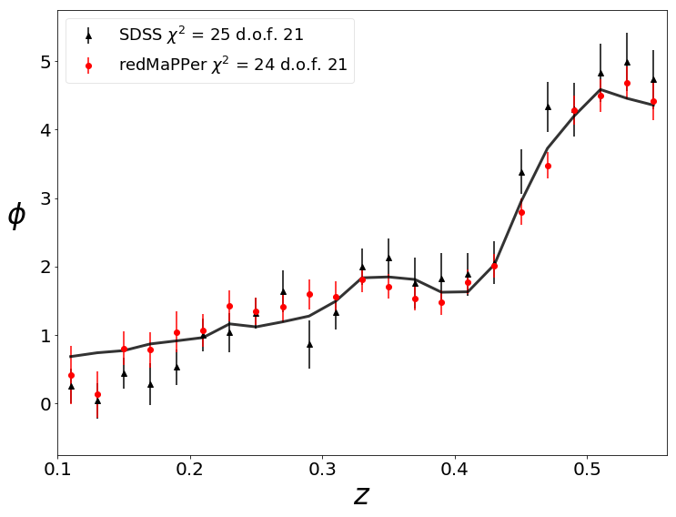
Figure 1: A comparison of the cross-correlation recovery of the SDSS redshift distribution with their spectroscopic redshifts. The solid line is the actual distribution of galaxies from spectroscopic data. The black points show the recovered SDSS redshift distribution using cross-correlation with a spectroscopic sample of SDSS galaxies as a reference sample. The red points show the corresponding redshift distribution when using redMaPPer galaxy clusters as the reference sample. Both sets of points account for the best-fit redshift evolution in the clustering bias.

We combine the CMASS and LOWZ samples and randomly split the galaxies into a reference sample containing 80% of the galaxies and an unknown sample containing the remaining 20%. The random selection ensures that the redshift distributions of the samples are identical. The reference sample is divided according to spectroscopic redshift into bins of width $\delta z=0.02$. Pair counts of the sample and randoms are counted as described above in Section 3. The pair counts are integrated into a single scalar from 100 kpc to 10 Mpc and weighted by $g(R)=R^{-1}$. In order to facilitate later comparison with redMaPPer clusters, which have a more limited redshift range than the spectroscopic sample, we normalize the distribution such that its integral from $z=0.1$ to $0.56$ is one. The highest redshift is set by the highest redshift for which we have enough redMaPPer clusters to obtain reasonable cross-correlation measurements. Covariances are estimated from jackknife samples over the survey footprint. We find that ignoring the bias evolution (setting $\gamma=0$) produces a poor fit between the clustering and spectroscopic measurements ($\chi^{2}/\mathrm{dof}=58/23$). We fit the bias evolution model described by Equation (27) and find that this brings our results into agreement ($\chi^{2}/\mathrm{dof}=25/21$), with $\gamma=-1.7\pm 0.5$. The results can be seen in the black triangles of Figure 1. These results validate our cross-correlation technique.

Next we repeat the same exercise, only now the reference objects are the redMaPPer clusters, and the unknown objects are the entire SDSS CMASS and LOWZ samples. We emphasize that our goal here is to test whether we can use redMaPPer clusters to measure redshift distributions through the cross-correlation, even if our signal includes scales well within the radius of a redMaPPer cluster. We again fit the same model to the clustering signal, and find that the cross-correlation method with redMaPPer clusters as a reference sample successfully recovers the correct redshift distribution of the unknown sample within noise ($\chi^{2}/\mathrm{dof}=24/21$), with $\gamma=-0.2\pm 0.4$. The results are shown as red circles in Figure 1. These results validate the idea that replacing spectroscopic reference samples with high-quality photometric reference samples is a viable approach to calibrating photometric redshift distributions via cross-correlations.

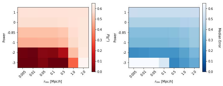
Figure 2: Effect of varying inner integration range $r_{\mathrm{min}}$ and weight power $\alpha$ on fit $\chi^{2}$ (Left) and median error (Right) for the recovery of the SDSS redshift distribution using SDSS galaxies. Setting the weight power too high will result in larger errors by emphasizing the weaker signal at larger scales, while setting the power too low will bias the measurement as extra weight is given to the non-linear regime. The power $\alpha=-0.85$ is included as a row because it is the slope of a powerlaw fit to the cross-correlations.

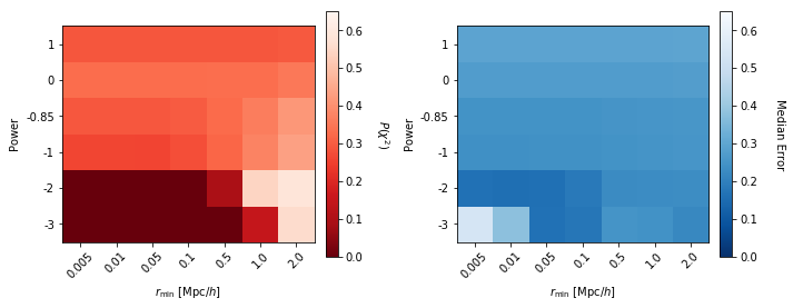
Figure 3: Effect of varying inner integration range $r_{\mathrm{min}}$ and weight power $\alpha$ on fit $\chi^{2}$ (Left) and median error (Right) for the recovery of the SDSS redshift distribution using redMaPPer galaxy clusters. As with Figure 2, the particular choice of hyperparameters can swing the recovered distribution’s fit and error properties significantly.

Cross-correlations convert angular clustering signal into estimates of the redshift distribution, but the error in clustering estimates varies with angular scale due to sample variance, shot noise, and survey systematics. Consequently, we test how our choice of weighting function affects the recovered redshift distribution, and how varying the radial range, particularly the inner radius, impacts our results. We consider simple power-law weighting functions $g(r)=r^{\alpha}$. We expect a priori that the optimal power will be close to the approximate power law exponent of the correlation function itself, $\alpha\sim-0.85$. Given this expectation, we expect the primary sensitivity to the radial range $r\in[r_{\rm{min}},r_{\rm{max}}]$ will be through the scale $r_{\rm{min}}$, which is why we focus on $r_{\rm{min}}$ in this study.

We find that there is a trade-off between bias and variance: varying the power of the weight function and the inner radius of the angular integration can significantly decrease the estimated covariance at the cost of noticeable biasing. Figures 2-3 summarize this trade-off. Each Figure has two colored grids showing the effect of varying the power of the weight function and the inner angular integration range on the recovered redshift distribution. In the left panel, we take the overall best $\chi^{2}$ fit and plot the probability $P_{k}(\chi^{2})$ that $\chi^{2}$ be larger than the observed value given the degrees of freedom in the analysis. When this probability is small, our recovered redshift distribution is not an acceptable fit to the data. In the right panel, we plot the median error of the recovered redshift distribution as estimated from jackknife samples, $\textrm{Median}\left(\sigma_{\phi}\right)$. For both the SDSS spectroscopic galaxy reference sample and the redMaPPer reference sample we find that $r_{\rm{min}}=0.1\ \rm{Mpc}$ and $\alpha=-1$ provide a nearly optimal tradeoff between accuracy and precision. However, we note that the specific response to variations in these parameters may differ in other samples.

5 Application to the Dark Energy Survey: Combining PHOTO-$z$’s with Cross-Correlation Methods

It is vital for DES to accurately constrain the redshift distributions of objects that are in tomographic bins for measurements of cosmic shear or baryon acoustic oscillations. Traditionally, one places galaxies into tomographic bins based on their photometrically-estimated probability distribution $P(z)$, and then one “stacks” these $P(z)$’s to estimate the redshift distribution of sources in a bin. The cross-correlation method as implemented here does not provide insight into which objects should go into each tomographic bin, but it does constrain the redshift distribution of the objects in each bin. Consequently, it can provide a critical systematics cross-check for photo-$z$ methods. This is especially desirable because the inputs and systematics that affect the cross-correlation method are largely independent of those affecting photo-$z$ methods. In particular, while spectroscopic redshift incompleteness is the primary difficulty affecting photo-$z$ algorithms, this systematic is completely irrelevant for cross-correlation.

In this Section we implement a cross-correlation measurement of the redshift distribution of NGMIX galaxies using redMaPPer clusters as the reference sample. The galaxies are placed into three tomographic bins with edges at $0.3,0.55,0.83,1.3$ according to the mean redshift of the SkyNet photo-$z$ code. While the NGMIX galaxies span a wide range of redshifts, we must limit our analyses to $0.2<z<0.84$, where we have redMaPPer clusters with reliable redshifts. Because of this limited redshift range, we do not perform the cross-correlation measurement on the third tomographic bin.

We repeat the same sort of cross-correlation analysis as in Section 4, where we use redMaPPer clusters to measure the redshift distribution. We set the power of the weighting term, $\alpha$ to -1 and integrate from 100 kpc to 10 Mpc. As with SDSS, we begin with the simple model in which $\gamma=0$, and the cross-correlation function is directly proportional to (and therefore an estimator of) $\phi(z)$.

We present the results of these analyses in the left column of Figure 4. Among the four codes we consider, only one has an acceptable $\chi^{2}$, namely BPZ. For the second tomographic bin, none of the photo-$z$ codes have an acceptable $\chi^{2}$. The $\chi^{2}$ of the predicted photo-$z$ distributions relative to the recovered redshift distribution are summarized in Table 1.

We seek to reconcile photo-$z$ and cross-correlation data where possible. As discussed in Bonnett et al. (2016), the primary source of systematic uncertainty affecting the photo-$z$ distributions is an overall photometric redshift bias. We utilize our cross-correlation data to calibrate this photometric redshift bias. In practice, this means replacing the photometric redshift distribution $\phi_{\rm{u}}(z)$ by a the function $\phi_{\rm{u}}(z-\Delta z)$ where $\Delta z$ is the photometric redshift bias of the algorithm in question. We write

$$\chi^{2}=\Delta w\hat{\Sigma}^{-1}\Delta w$$ (28)

where

$$\Delta w=\hat{w}-e^{k}\left(\frac{1+z}{1+z_{0}}\right)^{\gamma}\phi(z-\Delta z)$$ (29)

The quantity $k$ accounts for an overall relative normalization of the distributions, since we normalize $\hat{w}(z)$ to unity within the redshift range $[0.2,0.84]$, whereas $\phi(z)$ is normalized to unity within $[0,\infty]$. We also account for clustering bias evolution from Equation (24) via our parameterization of $(1+z)^{\gamma}$, which is normalized by $1+z_{0}$, where $z_{0}$ is chosen to be 0.52, the center of the cross-correlation redshift range. Because redshift biases and normalizations may change across tomographic bins, we define separate variables $k_{i},\Delta z_{i}$ for each tomographic bin. In contrast, we force each tomographic bin to simultaneously fit the same $\gamma$. This is consistent with our choice to encode all redshift evolution information into $\gamma$, although we note that clustering bias evolution may be induced by the photo-$z$ selection of the NGMIX galaxies into different tomographic bins. Not surprisingly, allowing for independent $\gamma$ in each of the tomographic bins can introduce large uncertainties in the recovered distributions since any individual tomographic bin is too narrow to properly constrain the redshift-dependent evolution of the clustering bias; one really needs the full range of redshifts probed by the data.

We also utilize our prior knowledge of the redshift distributions from the photo-$z$ codes. We model our prior on the redshift bias $\Delta z_{i}$ for each tomographic bin as a Gaussian centered on 0 with width $\sigma=0.05$ from prior analyses of photo-$z$ uncertainties from Bonnett et al. (2016). Thus, the expression we maximize is:

$$\ln\mathcal{L}=-\frac{1}{2}\chi^{2}\left(k_{i},\Delta z_{i},\gamma\right)-\sum_{j}\frac{1}{2}\frac{\Delta z_{j}^{2}}{2\times 0.05^{2}}$$ (30)

When cross-correlations are able to strongly constrain the redshift bias (as is the case here), the particular choice of prior does not matter. In cases when cross-correlations are unable to constrain the redshift bias we simply recover our prior. By using priors informed by photo-$z$ methods we open an avenue through which we may combine photo-$z$ and cross-correlation measurements.

We sample Equation (30) using emcee, an affine invariant Markov Chain Monte Carlo ensemble sampler (Foreman-Mackey et al., 2013). Results of these fits are presented in the right column of Figure 4 and in Table 1. Allowing for an overall redshift bias, all four photo-$z$ codes have an acceptable $\chi^{2}$, with TPZ resulting in the best fit. The good agreement between the codes is also apparent from Figure 4. By contrast, only one of the codes, BPZ, has an acceptable $\chi^{2}$ for the second tomographic bin. Figure 4 makes it apparent that most codes agree quite well on the shape of the photo-$z$ distribution in the vicinity of the average redshift of the galaxies in the bin, but differ significantly on the amplitude of a low-redshift tail in the distribution. The relatively small area of the DES SV region makes the correlation function measurements themselves very noisy in this regime, though the data does seem to indicate a preference for a larger tail, in agreement with the BPZ prediction. Future analyses from the full DES footprint should be able to clearly resolve this feature, and establish whether the “blips” seen in the lower right-hand panel of Figure 4 are real or just random fluctuations.

It is important to note that we also find discrepancies in our constraints on $\gamma\$ from the different photo-$z$ codes. This difference is easy to explain: the shape $\phi(z)$ of the distribution is clearly degenerate with $\gamma$. Since the different photo-$z$ codes have different shapes, $\gamma$ takes on a different value for each photo-$z$ code. This demonstrates that the shape of $\phi(z)$ estimated from the traditional photo-$z$ method constitutes an important systematic for our proposed method. Future work that seeks to implement the proposed method in cosmological analyses must properly quantify the associated systematic error, for instance through the use of simulated data.

Photo-$z$	Bin	$\chi^{2}_{\mathrm{raw},\mathrm{noRu}}$	$\chi^{2}_{\mathrm{cal},\mathrm{noRu}}$	$\mathrm{dof}$	$\Delta z_{\mathrm{noRu}}$	$\gamma_{\mathrm{noRu}}$
ANNZ2	1	$180$	$42$	$31$	$0.082\pm 0.011$	$0.6\pm 0.5$
ANNZ2	2	$64$	$57$	$31$	$-0.020\pm 0.014$	$0.6\pm 0.5$
BPZ	1	$39$	$38$	$31$	$-0.005\pm 0.006$	$0.1\pm 0.4$
BPZ	2	$87$	$43$	$31$	$-0.058\pm 0.011$	$0.1\pm 0.4$
SKYNET	1	$83$	$31$	$31$	$0.045\pm 0.008$	$0.5\pm 0.5$
SKYNET	2	$87$	$58$	$31$	$-0.018\pm 0.007$	$0.5\pm 0.5$
TPZ	1	$112$	$27$	$31$	$0.061\pm 0.009$	$0.5\pm 0.5$
TPZ	2	$86$	$59$	$31$	$-0.019\pm 0.008$	$0.5\pm 0.5$

Table 1: Table of results from fitting photo-$z$ codes to cross-correlation analyses from redMaPPer clusters with DES SV NGMIX galaxies by maximizing Equation (30). The ‘raw’ $\chi^{2}$ is the goodness of fit before allowing for an overall photometric bias of the photo-$z$ codes. The ‘cal’ $\chi^{2}$ value is that obtained after calibrating this bias using cross-correlations.

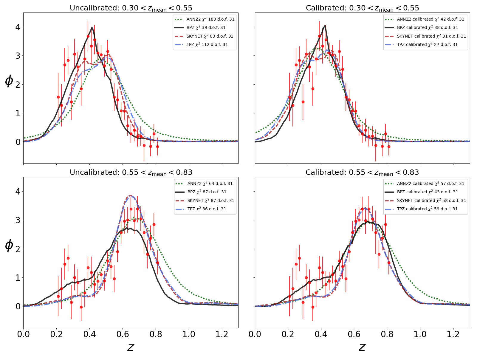
Figure 4: Redshift distribution of NGMIX galaxies using redMaPPer galaxy clusters before (left) and after (right) the calibration of Equations (28) and (29). Lines represent different photo-$z$ estimation codes, while the points represent the cross-correlation method. Each row of panels represent a different tomographic bin, with galaxies selected according to the SkyNet photo-$z$ method. Redshift distributions are normalized to one over the range of the cross-correlation sample $0.2<z<0.84$. The correction values are shown in Table 1. Note that in practice each photo-$z$ code modifies the predicted redshift distribution from the cross-correlation analysis through the bias evolution term. In order to make it easier to visually compare the different photo-$z$ codes, we apply the corrections associated with cross-correlations to the photo-$z$ redshift distributions, which allows a direct comparison with the cross-correlation data for all photo-$z$ codes.

Keeping in mind the above important caveat, it is reassuring to see that for the majority of the photo-$z$ codes the posterior on the redshift bias is less than 0.05 in magnitude, consistent with the expectations of Bonnett et al. (2016). In this context, it is also worth noting that our posteriors on $\Delta z$ measure the relative redshift bias between our unknown and reference samples. redMaPPer itself has photo-$z$ redshift biases that are unconstrained at the level of $\sigma_{\Delta z}\sim 0.003$. These are currently significantly smaller than the uncertainties from cross-correlations, but may need to be accounted for as the statistics of cross-correlations improve to DES Y5 levels.

Nevertheless, it is encouraging to see that the statistical precision from this analysis in the DES SV region ($\sim 139\ \mathrm{deg}^{2}$) is not far from what would be required for a DES Y5 ($\sim 5000\ \mathrm{deg}^{2}$) cosmology analysis. Of course, in practice, detailed simulation work will be required to properly characterize the systematic uncertainties associated with this type of analysis, and possibly motivate alterations to the simple algorithm proposed here. Motivated by these results, we have launched such a study in preparation for future DES cosmological analyses.

As a final test of our proposed analysis, we revisit the SDSS data set, and test our full algorithm there by calibrating the relative redshift bias between SDSS spectroscopic galaxies and redMaPPer clusters. As expected, we find the recovered redshift bias is consistent with zero $\Delta z=(-5.1\pm 4.6)\times 10^{-3}$, while the clustering bias evolution parameter $\gamma=-0.3\pm 0.5$. This level of uncertainty is consistent with a priori expectations of the redMaPPer redshift bias.

6 Cosmological Forecasts

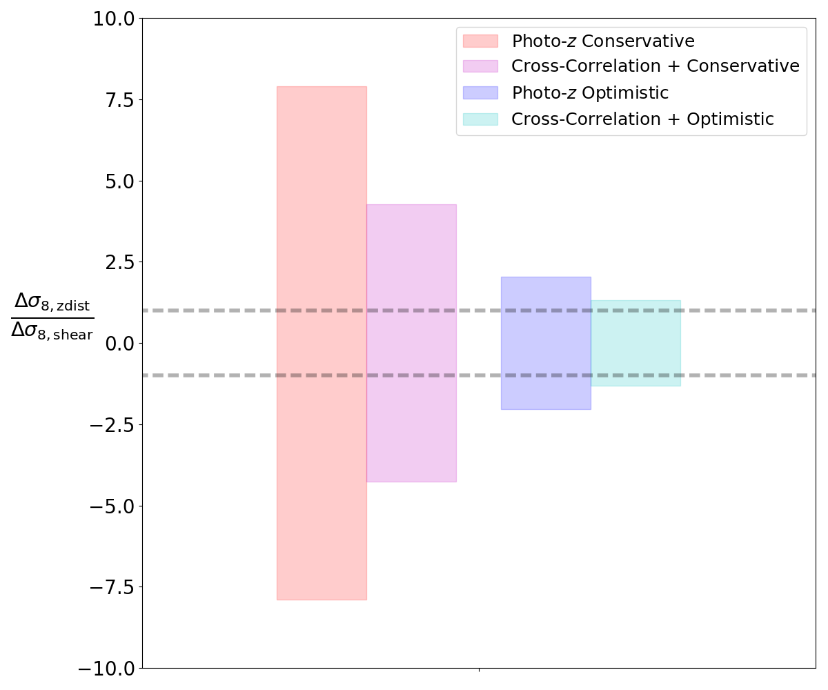
Figure 5: Ratio of the variation in $\sigma_{8}$ due to forecasted DES Y5 uncertainties from redshift distributions to shear statistical uncertainties. When this ratio is less than one, the uncertainty on $\sigma_{8}$ is dominated by errors in shape measurements; when the ratio is greater than one, errors from the redshift distribution dominate. The red (blue) band is the uncertainty due to the SkyNet photo-$z$ code with the conservative (optimistic) uncertainty $\sigma_{\Delta z}=0.05$ ($\sigma_{\Delta z}=0.02$) in the bias of the redshift distribution. The magenta (cyan) band is the residual uncertainty from using cross-correlations to constrain the redshift bias $\Delta z$. The grey dashed lines are guidelines for $\pm 1$. Tomographic constraints are limited by the lack of overlap with redMaPPer clusters in the third (highest redshift) tomographic bin, which prevents any cross-correlation calibration in that bin.

We now estimate the efficacy of cross-correlation redshift calibration for cosmological analyses of DES Y5 cosmic shear data. We start with the DES SV NGMIX cosmic shear two-point correlations. In order to perform our forecast, we must also specify a fiducial redshift distribution of sources. In keeping with the cosmic shear analysis of Becker et al. (2016), we take SkyNet as our fiducial redshift distribution. Here, we focus on the recovery of $\sigma_{8}$ (holding all other cosmological parameters fixed to their fiducial value) through the cosmology analysis pipeline used in Bonnett et al. (2016).

We focus on two key sources of uncertainty in cosmic shear measurements: errors in the measurement of the shear two point correlation function, and errors in our characterization of the redshift distribution from either photo-$z$ or cross-correlation systematics. We compare the posteriors in $\sigma_{8}$ for three different fiducial analyses. First, an analysis that includes only shape noise, and the source redshifts are assumed to be perfectly known. Second, an analysis that assumes no shape noise, but considers only the error in $\sigma_{8}$ introduced by an overall unknown photo-$z$ redshift bias with current photo-$z$ priors. Third, an analysis that assumes no shape noise, but considers the error in $\sigma_{8}$ introduced by unknown photo-$z$ redshift bias that is calibrated using cross-correlation.

To model our DES Y5 shear covariances, we scale the DES SV cosmic shear covariances by the area of the final survey, so that we divide the DES SV cosmic shear covariance matrix by $5000/139$, the ratio of DES Y5 to DES SV SPTE survey areas. Under the assumption that the galaxy density measured in SV will be equal to what we will have in Y5, this scaling is the improvement in statistical power from repeating our SV analysis over the full Y5 footprint.

To estimate the uncertainty in the recovered $\sigma_{8}$ due to an unknown photometric redshift bias with some prior and no cross-correlation data, we sample the redshift distributions $P(z-\Delta z)$ for the source galaxies, where $\Delta z$ is the redshift bias. We find the best fit $\sigma_{8}$ given the stacked $dN/dz$, and repeat our measurement 250 times, randomly drawing the redshift bias from the prior $\Delta z=0.00\pm 0.05$. This is the level of constraint if the same photo-$z$ algorithms from DES SV were used in DES Y5, and is hence our ‘conservative’ case. The standard deviation in the recovered $\sigma_{8}$ values is the uncertainty in $\sigma_{8}$ due to photometric redshift uncertainties. We also consider the case where photo-$z$ algorithms improve in the measurement of systematic redshift bias to $\sigma_{\Delta z}=0.02$. We refer this as our ‘optimistic’ scenario. Note ‘optimistic’ should not be confused with ‘unrealistic’; we expect future photo-$z$ codes to be able to reach this level of accuracy and precision.

To measure the effect of cross-correlation on the recovery of $\sigma_{8}$, we begin by estimating the uncertainty in the photometric redshift bias $\sigma_{\Delta z}$ as estimated from the cross-correlation method, as per our discussion in Section 5. This constraint depends on our fit for Equation (28). We scale our estimated errors $\hat{\Sigma}$ by the ratio of the survey areas between the DES Y5 and DES SV surveys (i.e. $5000/139$) to simulate the increase in signal. By then setting $\hat{\phi}=\phi$ and fitting as described in Section 5, we sample the space of solutions that are consistent with the cross-correlation method. These samples provide the redshift bias $\Delta z$ that goes into our cosmology analysis. This is roughly equivalent to the simpler method of scaling the errors in the photometric redshift biases in Table 1 by the square root of the ratio of the survey areas between the DES Y5 and DES SV surveys, but has the capability for incorporating more complex modifications of the redshift distribution in the future. When comparing the optimistic and conservative cases, we use the fact that we know from the photo-$z$ algorithms that $\sigma_{\Delta z}=(0.02,0.05)$ respectively by putting that information into our prior on the redshift bias via Equation (30). This makes a significant difference because the cross-correlation cannot calibrate the highest tomographic bin due to a lack of overlap with the redMaPPer clusters, and so we revert back to the prior there. In addition, using the sampling method used to characterize the cosmological uncertainties from photo-$z$, we also add a systematic redshift error $\sigma_{\Delta z}=0.003$ to our reference sample to account for the photometric redshift bias expected for redMaPPer clusters.

Figure 5 compares the errors in $\sigma_{8}$ from each of the three analyses considered above. We plot the ratio of the uncertainty on $\sigma_{8}$ arising from uncertainty in the mean of the redshift distribution (either from photo-$z$ or cross-correlation calibration) to the uncertainty on $\sigma_{8}$ arising from shape noise in the shear two point correlation function. When this ratio is less than one, the uncertainty on $\sigma_{8}$ is dominated by errors in shape measurements; when the ratio is greater than one, errors from the redshift distribution dominate. There is a noticeable improvement in the recovered cosmological parameters in our conservative analysis, but only a modest improvement in our optimistic scenario. This largely reflects the fact that our analyses does not constrain the highest tomographic redshift bin, which contains a large fraction of the cosmological signal. Nevertheless, it is very encouraging that even with this simple approach, and without incorporating the gains from high redshift cross-correlation analyses that may be enabled in the future, a combined photo-$z$ and cross-correlation analysis appears to have the potential to control photometric redshift systematics. Consequently, our results provide strong motivation for further investigations into the possible use of photometric cross-correlations for photo-$z$ calibration.

7 Summary and Conclusions

We examined the performance of cross-correlation methods when photometric redshifts are used instead of spectroscopic galaxies as a reference sample. We first verified that cross-correlation methods work with spectroscopic reference samples by looking at the cross-correlation of SDSS galaxies. We then found that redMaPPer galaxy clusters, despite having photometric redshifts, are also viable reference samples for measuring accurate redshift distributions.

Having validated our methodology on SDSS spectroscopic galaxies, we turned toward the DES NGMIX sample in the DES SV data set. There, we applied the cross-correlation method and compared our measured redshift distributions to those measured by a variety of photo-$z$ codes. We developed a formulation for calibrating systematic redshift biases in the photo-$z$ codes, using information from both the photo-$z$ and cross-correlation methods to improve the characterization of redshift distributions. We found that the recovered redshift bias relative to the cross-correlation measurement is typically less than $\sim 0.05$, with the posterior of the redshift bias being uncertain at the $\pm 0.01$ level. This level of uncertainty is comparable to the required DES Y5 uncertainty and should only improve with five more years of data. However, systematic errors, particularly from the evolution of clustering bias in both the source and reference samples, as well as from discrepancies between the shapes of the photo-$z$ and cross-correlation redshift distributions, need to be fully characterized for this method to be integrated into future cosmological analyses.

Finally, we extrapolated the recovered statistical uncertainties to DES Y5 data, and compared the statistical uncertainty in $\sigma_{8}$ from shape noise, the photometric uncertainties from a fiducial photo-$z$ algorithm with an unknown redshift bias at the $2\%$ level, and a fiducial analysis that includes calibrations from cross-correlations. The impact of the cross-correlation analysis depends on the uncertainty that traditional photo-$z$ algorithm can reach in the near future. Even in our optimistic scenario, however, cross-correlations provide a non-negligible improvement in the recovered cosmological constraints, while simultaneously providing a critical consistency test of the photo-$z$ calibration.

These results firmly establish the feasibility of using photometric samples as reference samples for calibrating photometric redshift distributions via cross-correlation, and provides strong motivation for more detailed simulation-based studies aimed at fully characterizing the systematic uncertainties in these methods. In particular, we have already seen hints that systematic uncertainties in the shape of the $\phi(z)$ estimated from traditional photo-$z$ methods can introduce systematics in the recovered photometric redshift bias. We are currently characterizing these systematics via numerical simulations for the DES Year 1 cosmology analysis (Gatti et al, in prep.). Similarly, it is not difficult to imagine modifications of the methodology adopted here that is more ideally suited to cosmological analyses. For example, cosmic shear analyses are primarily sensitive to photo-$z$ uncertainties through the photometric redshift bias and not the shape of the redshift distribution. The methods presented here could be tailored towards these goals by matching the means of the distributions while down-weighting the tails of the redshift distributions, thereby minimizing systematics associated with the detailed shape of $\phi(z)$. We are also exploring alternative high fidelity photometric reference samples such as the luminous red galaxy redMaGiC sample described in Rozo et al. (2016), which has considerably higher number density than redMaPPer clusters (Cawthon et al, in prep.). The fact that the cross-correlation provide a calibration tool that is demonstrably capable of reaching the necessary statistical precision for Stage III dark energy experiments is an important step forward in realizing the promise of the DES, and provides strong motivation for further studies of this method.

Affiliations

¹ Kavli Institute for Particle Astrophysics & Cosmology, P. O. Box 2450, Stanford University, Stanford, CA 94305, USA
² Institute of Space Sciences, IEEC-CSIC, Campus UAB, Carrer de Can Magrans, s/n, 08193 Barcelona, Spain
³ Kavli Institute for Cosmological Physics, University of Chicago, Chicago, IL 60637, USA
⁴ Institut de Física d’Altes Energies (IFAE), The Barcelona Institute of Science and Technology, Campus UAB, 08193 Bellaterra (Barcelona) Spain
⁵ Fermi National Accelerator Laboratory, P. O. Box 500, Batavia, IL 60510, USA
⁶ Institució Catalana de Recerca i Estudis Avançats, E-08010 Barcelona, Spain
⁷ SLAC National Accelerator Laboratory, Menlo Park, CA 94025, USA
⁸ Department of Physics, University of Arizona, Tucson, AZ 85721, USA
⁹ Center for Cosmology and Astro-Particle Physics, The Ohio State University, Columbus, OH 43210, USA
¹⁰ Department of Physics, The Ohio State University, Columbus, OH 43210, USA
¹¹ Cerro Tololo Inter-American Observatory, National Optical Astronomy Observatory, Casilla 603, La Serena, Chile
¹² Department of Physics & Astronomy, University College London, Gower Street, London, WC1E 6BT, UK
¹³ Department of Physics and Electronics, Rhodes University, PO Box 94, Grahamstown, 6140, South Africa
¹⁴ LSST, 933 North Cherry Avenue, Tucson, AZ 85721, USA
¹⁵ CNRS, UMR 7095, Institut d’Astrophysique de Paris, F-75014, Paris, France
¹⁶ Sorbonne Universités, UPMC Univ Paris 06, UMR 7095, Institut d’Astrophysique de Paris, F-75014, Paris, France
¹⁷ Laboratório Interinstitucional de e-Astronomia - LIneA, Rua Gal. José Cristino 77, Rio de Janeiro, RJ - 20921-400, Brazil
¹⁸ Observatório Nacional, Rua Gal. José Cristino 77, Rio de Janeiro, RJ - 20921-400, Brazil
¹⁹ Department of Astronomy, University of Illinois, 1002 W. Green Street, Urbana, IL 61801, USA
²⁰ National Center for Supercomputing Applications, 1205 West Clark St., Urbana, IL 61801, USA
²¹ Department of Physics and Astronomy, University of Pennsylvania, Philadelphia, PA 19104, USA
²² Department of Physics, IIT Hyderabad, Kandi, Telangana 502285, India
²³ Instituto de Fisica Teorica UAM/CSIC, Universidad Autonoma de Madrid, 28049 Madrid, Spain
²⁴ Department of Astronomy, University of Michigan, Ann Arbor, MI 48109, USA
²⁵ Department of Physics, University of Michigan, Ann Arbor, MI 48109, USA
²⁶ Institute of Astronomy, University of Cambridge, Madingley Road, Cambridge CB3 0HA, UK
²⁷ Kavli Institute for Cosmology, University of Cambridge, Madingley Road, Cambridge CB3 0HA, UK
²⁸ Universitäts-Sternwarte, Fakultät für Physik, Ludwig-Maximilians Universität München, Scheinerstr. 1, 81679 München, Germany
²⁹ Astronomy Department, University of Washington, Box 351580, Seattle, WA 98195, USA
³⁰ Santa Cruz Institute for Particle Physics, Santa Cruz, CA 95064, USA
³¹ Australian Astronomical Observatory, North Ryde, NSW 2113, Australia
³² Argonne National Laboratory, 9700 South Cass Avenue, Lemont, IL 60439, USA
³³ Departamento de Física Matemática, Instituto de Física, Universidade de São Paulo, CP 66318, São Paulo, SP, 05314-970, Brazil
³⁴ George P. and Cynthia Woods Mitchell Institute for Fundamental Physics and Astronomy, and Department of Physics and Astronomy, Texas A&M University, College Station, TX 77843, USA
³⁵ Department of Astronomy, The Ohio State University, Columbus, OH 43210, USA
³⁶ Department of Astrophysical Sciences, Princeton University, Peyton Hall, Princeton, NJ 08544, USA
³⁷ Jet Propulsion Laboratory, California Institute of Technology, 4800 Oak Grove Dr., Pasadena, CA 91109, USA
³⁸ Department of Physics and Astronomy, Pevensey Building, University of Sussex, Brighton, BN1 9QH, UK
³⁹ Centro de Investigaciones Energéticas, Medioambientales y Tecnológicas (CIEMAT), Madrid, Spain
⁴⁰ School of Physics and Astronomy, University of Southampton, Southampton, SO17 1BJ, UK
⁴¹ Instituto de Física Gleb Wataghin, Universidade Estadual de Campinas, 13083-859, Campinas, SP, Brazil
⁴² Computer Science and Mathematics Division, Oak Ridge National Laboratory, Oak Ridge, TN 37831
⁴³ Institute of Cosmology & Gravitation, University of Portsmouth, Portsmouth, PO1 3FX, UK
⁴⁴ Department of Physics, Stanford University, 382 Via Pueblo Mall, Stanford, CA 94305, USA

References

- Alam et al. (2015) Alam S., et al., 2015, ApJS, 219, 12
- Asorey et al. (2016) Asorey J., Carrasco Kind M., Sevilla-Noarbe I., Brunner R. J., Thaler J., 2016, MNRAS, 459, 1293
- Becker et al. (2016) Becker M. R., et al., 2016, Phys. Rev. D, 94, 022002
- Bell et al. (2004) Bell E. F., et al., 2004, ApJ, 608, 752
- Benítez (1999) Benítez N., 1999, in Weymann R., Storrie-Lombardi L., Sawicki M., Brunner R., eds, Astronomical Society of the Pacific Conference Series Vol. 191, Photometric Redshifts and the Detection of High Redshift Galaxies. p. 31
- Benjamin et al. (2010) Benjamin J., van Waerbeke L., Ménard B., Kilbinger M., 2010, MNRAS, 408, 1168
- Bertin (2010) Bertin E., 2010, SWarp: Resampling and Co-adding FITS Images Together, Astrophysics Source Code Library (ascl:1010.068)
- Bertin (2011) Bertin E., 2011, in Evans I. N., Accomazzi A., Mink D. J., Rots A. H., eds, Astronomical Society of the Pacific Conference Series Vol. 442, Astronomical Data Analysis Software and Systems XX. p. 435
- Bertin & Arnouts (1996) Bertin E., Arnouts S., 1996, A&AS, 117, 393
- Bonnett (2015) Bonnett C., 2015, MNRAS, 449, 1043
- Bonnett et al. (2016) Bonnett C., et al., 2016, Phys. Rev. D, 94, 042005
- Bower et al. (1992) Bower R. G., Lucey J. R., Ellis R. S., 1992, MNRAS, 254, 601
- Carlstrom et al. (2011) Carlstrom J. E., et al., 2011, PASP, 123, 568
- Carrasco Kind & Brunner (2013) Carrasco Kind M., Brunner R., 2013, TPZ: Trees for Photo-Z, Astrophysics Source Code Library (ascl:1304.011)
- Carrasco Kind & Brunner (2014) Carrasco Kind M., Brunner R., 2014, MLZ: Machine Learning for photo-Z, Astrophysics Source Code Library (ascl:1403.003)
- Choi et al. (2016) Choi A., et al., 2016, MNRAS, 463, 3737
- Coe et al. (2006) Coe D., Benítez N., Sánchez S. F., Jee M., Bouwens R., Ford H., 2006, AJ, 132, 926
- Cunha et al. (2009) Cunha C. E., Lima M., Oyaizu H., Frieman J., Lin H., 2009, MNRAS, 396, 2379
- Desai et al. (2012) Desai S., et al., 2012, ApJ, 757, 83
- Flaugher et al. (2015) Flaugher B., et al., 2015, AJ, 150, 150
- Foreman-Mackey et al. (2013) Foreman-Mackey D., Hogg D. W., Lang D., Goodman J., 2013, PASP, 125, 306
- Graff et al. (2014) Graff P., Feroz F., Hobson M. P., Lasenby A., 2014, MNRAS, 441, 1741
- Hildebrandt et al. (2017) Hildebrandt H., et al., 2017, MNRAS, 465, 1454
- Hinshaw et al. (2013) Hinshaw G., et al., 2013, ApJS, 208, 19
- Hogg & Lang (2013) Hogg D. W., Lang D., 2013, PASP, 125, 719
- Jarvis et al. (2004) Jarvis M., Bernstein G., Jain B., 2004, MNRAS, 352, 338
- Jarvis et al. (2016) Jarvis M., et al., 2016, MNRAS, 460, 2245
- Johnson et al. (2017) Johnson A., et al., 2017, MNRAS, 465, 4118
- Landy & Szalay (1993) Landy S. D., Szalay A. S., 1993, ApJ, 412, 64
- Lee et al. (2016) Lee B. C. G., Budavári T., Basu A., Rahman M., 2016, AJ, 152, 155
- Lima et al. (2008) Lima M., Cunha C. E., Oyaizu H., Frieman J., Lin H., Sheldon E. S., 2008, MNRAS, 390, 118
- Matthews & Newman (2010) Matthews D. J., Newman J. A., 2010, ApJ, 721, 456
- Matthews & Newman (2012) Matthews D. J., Newman J. A., 2012, ApJ, 745, 180
- McLeod et al. (2016) McLeod M., Balan S. T., Abdalla F. B., 2016
- McQuinn & White (2013) McQuinn M., White M., 2013, MNRAS, 433, 2857
- Ménard et al. (2013) Ménard B., Scranton R., Schmidt S., Morrison C., Jeong D., Budavari T., Rahman M., 2013, preprint, (arXiv:1303.4722)
- Morrison et al. (2017) Morrison C. B., Hildebrandt H., Schmidt S. J., Baldry I. K., Bilicki M., Choi A., Erben T., Schneider P., 2017, MNRAS, 467, 3576
- Newman (2008) Newman J. A., 2008, ApJ, 684, 88
- Rahman et al. (2015) Rahman M., Ménard B., Scranton R., Schmidt S. J., Morrison C. B., 2015, MNRAS, 447, 3500
- Rahman et al. (2016) Rahman M., Mendez A. J., Ménard B., Scranton R., Schmidt S. J., Morrison C. B., Budavári T., 2016, MNRAS, 460, 163
- Rozo et al. (2015a) Rozo E., Rykoff E. S., Bartlett J. G., Melin J.-B., 2015a, MNRAS, 450, 592
- Rozo et al. (2015b) Rozo E., Rykoff E. S., Becker M., Reddick R. M., Wechsler R. H., 2015b, MNRAS, 453, 38
- Rozo et al. (2016) Rozo E., et al., 2016, MNRAS, 461, 1431
- Rykoff et al. (2014) Rykoff E. S., et al., 2014, ApJ, 785, 104
- Rykoff et al. (2016) Rykoff E. S., et al., 2016, ApJS, 224, 1
- Sadeh et al. (2016) Sadeh I., Abdalla F. B., Lahav O., 2016, PASP, 128, 104502
- Sánchez et al. (2014) Sánchez C., et al., 2014, MNRAS, 445, 1482
- Schmidt et al. (2013) Schmidt S. J., Ménard B., Scranton R., Morrison C., McBride C. K., 2013, MNRAS, 431, 3307
- Schmidt et al. (2015) Schmidt S. J., Ménard B., Scranton R., Morrison C. B., Rahman M., Hopkins A. M., 2015, MNRAS, 446, 2696
- Schulz (2010) Schulz A. E., 2010, ApJ, 724, 1305
- Scottez et al. (2016) Scottez V., et al., 2016, MNRAS, 462, 1683
- Scottez et al. (2017) Scottez V., Benoit-Lévy A., Coupon J., Ilbert O., Mellier Y., 2017, preprint
- Sevilla et al. (2011) Sevilla I., et al., 2011, preprint, (arXiv:1109.6741)
- Sheldon (2014) Sheldon E. S., 2014, MNRAS, 444, L25
- Sun et al. (2015) Sun L., Zhan H., Tao C., 2015, preprint, (arXiv:1512.00600v1)
- van Daalen & White (2017) van Daalen M. P., White M., 2017, preprint, (arXiv:1703.05326)
- Zuntz et al. (2013) Zuntz J., Kacprzak T., Voigt L., Hirsch M., Rowe B., Bridle S., 2013, MNRAS, 434, 1604