A bijection for essentially 4-connected toroidal triangulations

Abstract

Transversal structures (also known as regular edge labelings) are combinatorial structures defined over 4-connected plane triangulations with quadrangular outer-face. They have been intensively studied and used for many applications (drawing algorithm, random generation, enumeration…). In this paper we introduce and study a generalization of these objects for the toroidal case. Contrary to what happens in the plane, the set of toroidal transversal structures of a given toroidal triangulation is partitioned into several distributive lattices. We exhibit a subset of toroidal transversal structures, called balanced, and show that it forms a single distributive lattice. Then, using the minimal element of the lattice, we are able to enumerate bijectively essentially 4-connected toroidal triangulations.

1 Introduction

A graph embedded on a surface is called a map on this surface if all its faces are homeomorphic to open disks. Maps are considered up to homeomorphism. A map is a triangulation if all its faces have size three. Given a graph embedded on a surface, a contractible loop is an edge enclosing a region homeomorphic to an open disk. Two edges of an embedded graph are called homotopic multiple edges if they have the same extremities and their union encloses a region homeomorphic to an open disk. In this paper, we restrict ourselves to graphs embedded on surfaces that do not have contractible loops nor homotopic multiple edges. Note that this is a weaker assumption, than the graph being simple, i.e. not having loops nor multiple edges. In this paper we distinguish cycles from closed walk as cycles have no repeated vertices. A contractible cycle is a cycle enclosing a region homeomorphic to an open disk. A triangle (resp. quadrangle) of a map is a closed walk of length three (resp. four) that delimits on one side a region homeomorphic to an open disk. This region is called the interior of the triangle (resp. quadrangle). Note that a triangle is not necessarily a face of the map as its interior may be not empty. Note also that a triangle is not necessarily a cycle since non-contractible loops are allowed. A unicellular map is a map with only one face, which corresponds to the natural generalization of planar trees when going to higher genus, see [CMS09, Cha11].

In this paper we consider finite maps. We denote by $n$ be the number of vertices and $m$ the number of edges of a graph. Given a graph embedded on a surface, we use $f$ for the number of faces. Euler’s formula says that any map on an orientable surface of genus $g$ satisfies $n-m+f=2-2g$. In particular, the plane is the surface of genus $0$, the torus the surface of genus $1$, the double torus the surface of genus $2$, etc. By Euler’s formula, a toroidal triangulation with $n$ vertices has exactly $3n$ edges and $2n$ faces.

The universal cover of the torus is a surjective mapping $p$ from the plane to the torus that is locally a homeomorphism. If the torus is represented by a hexagon (or parallelogram) in the plane whose opposite sides are pairwise identified, then the universal cover of the torus is obtained by replicating the hexagon (or parallelogram) to tile the plane.

A graph is $k$-connected if it has at least $k+1$ vertices and if it stays connected after removing any $k-1$ vertices. Extending the notion of essentially 2-connectedness defined in [MR98], we say that a toroidal map $G$ is essentially $k$-connected if its universal cover $G^{\infty}$ is $k$-connected (note that this is different from $G$ being $k$-connected). This paper is focused on the study of essentially 4-connected toroidal triangulations via generalizing transversal structures to the toroidal case.

Transversal structures are originally defined on $4$-connected planar triangulations with four vertices on the outer face. They have been introduced by Kant et He [KH97] (under the name regular edge labelings) for graph drawing applications of planar maps [KH97, Fus09]. Deep combinatorial properties of these objects have been studied later by Fusy [Fus09] with numerous other applications like encoding, enumeration, random generation, etc. Indeed, in the planar case, transversal structures are strongly related to a more general object called $\alpha$-orientations by Felsner [Fel04]. Consider a graph $G$, with vertex set $V$, and a function $\alpha:V\to\mathbb{N}$. An orientation of $G$ is an $\alpha$-orientation if, for every vertex $v\in V$, its outdegree $d^{+}(v)$ equals $\alpha(v)$. For a fix planar map $G$ and function $\alpha$, the set of $\alpha$-orientations of $G$ carries a structure of distributive lattice (see [Fel04] and older related results [Pro93, dM94]) In the planar case, there is a bijection between transversal structure of a planar map and $4$-orientations of the corresponding angle map. Thus the set of transversal structures of a given planar map also carries a structure of distributive lattice whose minimal element plays a crucial role for bijection purpose.

In the toroidal case, things are more complicated since the bijection of transversal structures with $4$-orientations is not valid anymore. Moreover the set of $\alpha$-orientations of a given toroidal map is now partitioned into several distributive lattices (see [Pro93, GKL16]) contrarily to the planar case where there is only one lattice and thus only one minimal element. Similar issues appear in the study of Schnyder woods and corresponding $3$-orientations of toroidal triangulations. In a series of papers [GL14, GKL16, DGL17] (see also the HDR manuscript of the second author [Lév17] which present these three papers in a unified way), these problems are solved by highlighting a particular global property, called “balanced” in [Lév17], that a $3$-orientation may have.

By following the same guidelines here, we are able to identify, in Section 2, a similar “balanced” property for $4$-orientations of the angle map. These so-called balanced $4$-orientations form the core object of study of this paper. Whereas not all $4$-orientations corresponds to transversal structures, we show in Section 3 that all balanced ones correspond to transversal structures. The existence of balanced objects for essentially 4-connected toroidal triangulations is proved in Section 4 by edge contraction. The set of $4$-orientations of the angle map of a given essentially $4$-connected toroidal triangulation is partitioned into distributive lattices but all the balanced $4$-orientations are contained in the same lattice, as shown in Section 5. The minimal element of this “balanced lattice” as some important properties that are used in Section 6 to obtain a bijection between essentially $4$-connected toroidal triangulations and some toroidal unicellular maps. Then this bijection is used in Section 7 to enumerate essentially $4$-connected toroidal triangulations.

2 Angle map, transversal structure, balanced property and universal cover

2.1 Angle map and balanced 4-orientations

Consider a toroidal triangulation $G$. The angle map $A(G)$ of $G$ is the bipartite map obtained from a simultaneous embedding of vertices of $G$ and $G^{*}$ such that vertices of $G^{*}$ are embedded inside faces of $G$ and vice-versa, and for each angle of a vertex $v$ incident to a face $v^{*}$ there is an edge between $v$ and $v^{*}$. Hence, $A(G)$ is a bipartite map with one part consisting of primal-vertices and the other part consisting of dual-vertices. Each dual-vertex has degree three and each face of $A(G)$ is a quadrangle that consists of two primal-vertices and two dual-vertices.

Figure 1 gives an example of a toroidal triangulation and its angle map, primal-vertices are black and dual-vertices are white (this serves as a convention for the entire paper).

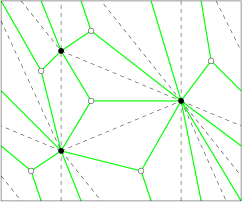
Figure 1: A toroidal triangulation and its angle map.

An orientation of the edges of $A(G)$ is called a $4$-orientation if every primal-vertex has outdegree exactly $4$ and every dual-vertex has outdegree exactly $1$. Euler’s formula says that for a toroidal triangulation we have $2n=f$, so the number of edges of the angle map is $3f=4n+f$. Thus Euler’s formula is “compatible” with existence of $4$-orientations for angle maps of toroidal triangulations ($4n$ outgoing edges for primal-vertices and $f$ outgoing edges for dual-vertices.

Consider an orientation of the edges of $A(G)$ and a cycle $C$ of $G$ together with a direction of traversal. We define $\gamma(C)$ by:

$$\gamma(C)=\#\ \text{edges of $A(G)$ leaving $C$ on its right}-\#\ \text{edges of $A(G)$ leaving $C$ on its left}.$$

Then we can define balanced orientations:

Definition 1 (Balanced $4$-orientation)

A $4$-orientation of $A(G)$ is balanced if every non-contractible cycle $C$ of $G$ satisfies $\gamma(C)=0$.

Figure 2 gives two examples of $4$-orientations of the same angle map of a toroidal triangulation. On the left example, the vertical loop of the triangulation, with upward direction of traversal, has $\gamma=2$, thus the orientation is not balanced. On the right example, one can check that $\gamma=0$ for any non-contractible cycle (note that we prove latter that it suffices to check that $\gamma$ equals $0$ for a vertical cycle and a horizontal cycle to be balanced, see Lemma 14).

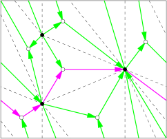
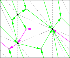
Non-balanced	Balanced

Figure 2: Two different $4$-orientations of the angle map of a toroidal triangulation, exactly one of which is balanced. One is obtain from the other by flipping the magenta cycle.

Balanced $4$-orientations are the main ingredient of this paper. Among all, we show that an essentially $4$-connected toroidal triangulation admits a balanced $4$-orientation of its angle map, and we exhibit the structure of distributive lattice of the set of all these balanced orientations.

In the next section we show how $4$-orientations are related to transversal structures.

2.2 Balanced transversal structures

Transversal structures have been defined originally in the planar case (see [KH97, Fus09]) and we propose the following generalization to the toroidal case.

First we define the following local rule:

Definition 2 (Transversal structure local property)

Given a map $G$, a vertex $v$ and an orientation and coloring of the edges incident to $v$ with the colors blue and red, we say that $v$ satisfies the transversal structure local property (or local property for short) if the edges around $v$ form in counterclockwise order a non-empty interval of outgoing edges of color blue, a non-empty interval of outgoing edges of color red, a non-empty interval of incoming edges of color blue, a non-empty interval of incoming edges of color red (see Figure 3).

Figure 3: The (transversal structure) local property.

Then the definition of toroidal transversal structure is the following:

Definition 3 (Toroidal transversal structure)

Given a toroidal map $G$, a toroidal transversal structure of $G$ is an orientation and coloring of the edges of $G$ with the colors blue and red where every vertex satisfies the transversal structure local property.

See Figure 4 for an example of a toroidal transversal structure of the triangulation of Figure 1.

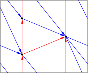
Figure 4: Example of a toroidal transversal structure.

From a toroidal transversal structure of a toroidal triangulation $G$, one can deduce a $4$-orientation of its angle map $A(G)$ by the following rule applied around each primal-vertex (see Figure 5): an edge $e$ of $A(G)$ is oriented toward its primal-vertex if the two primal edges around $e$ share the same color otherwise $e$ is oriented toward its dual-vertex. The fact that primal-vertices of $A(G)$ gets outdegree $4$ is clear by the definition of transversal structure. The fact that dual-vertices gets outdegree $1$ is due to the property that, by the local rule, all (triangular) faces of $G$ looks like one of Figure 6 where the four cases are symmetric by rotation of the order (outgoing blue, outgoing red, incoming blue, incoming red).

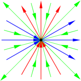
Figure 5: Orientation of the angle map corresponding to a transversal structure.

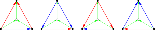
Figure 6: The four possible faces in a transversal structure and the corresponding orientation of the angle map.

The $4$-orientation on the right of Figure 2 is the one obtained from Figure 4 by the rule of Figure 5.

In the plane, there is a bijection between transversal structures of a map and $4$-orientations of its angle map (see [Fus09]). This is not true in the toroidal case. For example, there is no transversal structure associated to the (non-balanced) $4$-orientation of the left of Figure 2.

Like it has been done in [GKL16, Theorems 3.7] (see also [Lév17, Section 4.2]) for toroidal Schnyder woods, it is possible to characterize which $4$-orientations of the angle map of a toroidal triangulation corresponds a transversal structure. This is done in Section 3. A consequence of such a characterization (see Corollary 1) is that if a $4$-orientation is balanced, then it corresponds to a transversal structure.

So the balanced property is a sufficient condition to corresponds to a transversal structure. Note that it is not a necessary condition. Figure 7 gives an example of a transversal structure of a toroidal triangulation whose corresponding $4$-orientation of its angle map is not balanced. The horizontal cycle (with direction of traversal from right to left) has $\gamma=8$.

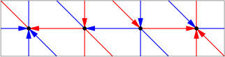
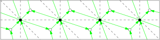
Figure 7: Example of a toroidal transversal structure whose corresponding $4$-orientation of angle map is not balanced.

Note also that in the plane, transversal structures can be defined by omitting the orientation of the edges in the local property since there is a bijection with $4$-orientations of the angle map. Again, this is not the case in the torus. Figure 8 gives an example of a blue/red coloring of the edges of a toroidal triangulation satisfying the local rule of transversal structure, without the orientation of the edges. It is not possible to orient the edges so this coloring becomes a toroidal transversal structure. The corresponding orientation of the angle map is still a $4$-orientation. Note that by gluing two copies of this example, one obtains Figure 7 that becomes orientable.

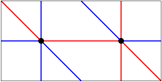
Figure 8: Example of a blue/red coloring of the edges of a toroidal triangulation satisfying the local rule of transversal structure, without the orientation of the edges, and that is not a transversal structure.

We give the following definition of balanced for toroidal transversal structure:

Definition 4 (Balanced toroidal transversal structure)

A toroidal transversal structure is balanced if its corresponding $4$-orientation of angle map is balanced.

Figure 4 gives an example of a balanced toroidal transversal structure. The corresponding $4$-orientation of the angle map is the balanced $4$-orientation of the right of Figure 2.

In section 4 we prove the existence of balanced toroidal transversal structure for essentially 4-connected toroidal triangulations. This implies the existence of balanced $4$-orientations for their angle maps.

2.3 Transversal structures in the universal cover

Consider a toroidal map $G$ and its universal cover $G^{\infty}$. Note that $G$ does not have contractible loops nor homotopic multiple edges if and only if $G^{\infty}$ is simple.

We need the following lemma from [GKL16]:

Lemma 1 ([GKL16, Lemma 2.8])

Suppose that for a finite set of vertices $X$ of $G^{\infty}$, the graph $G^{\infty}\setminus X$ is not connected. Then $G^{\infty}\setminus X$ has a finite connected component.

Suppose now that $G$ is a toroidal triangulation given with a transversal structure. Consider the natural extension of the transversal structure of $G$ to $G^{\infty}$, where an edge of $G^{\infty}$ receive the orientation and color of the corresponding edge in $G$. Let $G^{\infty}_{B}$, $G^{\infty}_{R}$ be the directed subgraphs of $G^{\infty}$ induced by the edges of color blue and red, respectively. The graphs $(G^{\infty}_{B})^{-1}$ and $(G^{\infty}_{R})^{-1}$ are the graphs obtained from $G^{\infty}_{B}$ and $G^{\infty}_{R}$ by reversing all their edges. Similarly to what happens for Schnyder woods (see [Lév17, Lemma 6]) we have the following property:

Lemma 2

The graphs $G^{\infty}_{B}\cup G^{\infty}_{R}$ and $G^{\infty}_{B}\cup(G^{\infty}_{R})^{-1}$ contain no directed cycle.

Proof. Let us prove the property for $G^{\infty}_{B}\cup G^{\infty}_{R}$, the proof is similar for $G^{\infty}_{B}\cup(G^{\infty}_{R})^{-1}$. Suppose by contradiction that there is a directed cycle in $G^{\infty}_{B}\cup G^{\infty}_{R}$. Let $C$ be such a cycle containing the minimum number of faces in the finite map $D$ with border $C$. Suppose without loss of generality that $C$ turns around $D$ counterclockwisely. By the transversal structure local property, every vertex of $D$ has at least one outgoing edge of color red in $D$. So there is a cycle of color red in $D$ and this cycle is $C$ by minimality of $C$. Every vertex of $D$ has at least one incoming edge of color blue in $D$. So, again by minimality of $C$, the cycle $C$ is a cycle of color blue. This contradicts the fact that edges of $G^{\infty}$ have a unique color. $\Box$

For a vertex $v$ of $G^{\infty}$, we define $P_{0}(v)$ (resp. $P_{1}(v)$, $P_{2}(v)$, $P_{3}(v)$) the subgraph of $G^{\infty}$ obtained by keeping all the edges that are on an oriented path of $G^{\infty}_{B}$ (resp. $G^{\infty}_{R}$, $(G^{\infty}_{B})^{-1}$, $(G^{\infty}_{R})^{-1}$) starting at $v$. Then we have the following lemma:

Lemma 3

For every vertex $v$ and $i,j\in\{0,1,2,3\}$, $i\neq j$, the two subgraphs $P_{i}(v)$ and $P_{j}(v)$ of $G^{\infty}$ have $v$ as only common vertex.

Proof. If $P_{i}(v)$ and $P_{j}(v)$ intersect on two vertices, then $G^{\infty}_{B}\cup G^{\infty}_{R}$ or $G^{\infty}_{B}\cup(G^{\infty}_{R})^{-1}$ contains a directed cycle, contradicting Lemma 2. $\Box$

Now we can prove that the existence of a transversal structure for a toroidal triangulation implies the $4$-connectedness of its universal cover:

Lemma 4

If a toroidal triangulation admits a toroidal transversal structure, then it is essentially 4-connected.

Proof. Suppose by contradiction that there exists three vertices $x,y,z$ of $G^{\infty}$ such that $G^{\prime}=G^{\infty}\setminus\{x,y,z\}$ is not connected. Then, by Lemma 1, the graph $G^{\prime}$ has a finite connected component $R$. Let $v$ be a vertex of $R$. By Lemma 2, for $i\in\{0,1,2,3\}$, the infinite and acyclic graph $P_{i}(v)$ does not lie in $R$ so it intersects one of $x,y,z$. So for two distinct $i,j$, the two graphs $P_{i}(v)$ and $P_{j}(v)$ intersect on a vertex distinct from $v$, a contradiction to Lemma 3. $\Box$

In Section 4, we prove the converse of Lemma 4 (see Theorem 2).

A separating triangle of a map is a triangle whose interior is non empty. We have the following equivalence:

Lemma 5

A toroidal triangulation is essentially $4$-connected if and only if its universal cover has no separating triangle.

Proof. ($\Longrightarrow$) Consider an essentially $4$-connected toroidal triangulation $G$. So $G^{\infty}$ is $4$-connected. If $G^{\infty}$ has a separating triangle, then, the three vertices of the triangle form a contradiction to the $4$-connectedness of $G^{\infty}$. So $G^{\infty}$ has no separating triangle.

($\Longleftarrow$) Consider a toroidal triangulation $G$ such that $G^{\infty}$ has no separating triangle. Suppose by contradiction that $G^{\infty}$ is not $4$-connected. Then there exists a set of $3$ vertices $X=\{x,y,z\}$ such that $G^{\infty}\setminus X$ is not connected. By Lemma 1, the graph $G^{\infty}\setminus X$ has a finite connected component $R$. Let $F$ be the face of $G^{\infty}\setminus R$ containing $R$. If $F$ has length $1$ or $2$ then $G^{\infty}$ is not simple, a contradiction. If $F$ has size $3$, then $F$ is a separating triangle of $G^{\infty}$, a contradiction. So $F$ has size at least $4$. Then there exists a vertex $v$ in $F\setminus X$. There is no edges between $v$ and $R$ and thus in $G^{\infty}$ the face incident to $v$ and $R$ has length strictly more than $3$, a contradiction of $G$ being a triangulation. $\Box$

We say that a quadrangle is maximal (by inclusion) if its interior is not strictly contained in the interior of another quadrangle.

Lemma 6

Consider an essentially $4$-connected toroidal triangulation $G$ and an edge $e$ of $G$. Then there is a unique maximal quadrangle of $G$ whose interior contains $e$.

Proof. Since $G$ is a toroidal triangulation, $e$ is clearly contained in the interior of the quadrangle bordering its two incident faces. So $e$ is contained in a maximal quadrangle.

Suppose by contradiction that there exist two distinct maximal quadrangles $Q,Q^{\prime}$ such that their interiors contain $e$. Let $R,R^{\prime}$ denote the interior of $Q,Q^{\prime}$ respectively. The two region $R,R^{\prime}$ are distinct, both contain the two faces incident to $e$ plus some other faces. If there is an edge in $R$ (resp. $R^{\prime}$) connecting two opposite vertices of $Q$ (resp. $Q^{\prime}$), then $G^{\infty}$ contains a separating triangle, a contradiction of $G$ being essentially $4$-connected and Lemma 5. Then since there is no homotopic multiple edges in $G$, there is at least one or two vertices of $Q$ (resp $Q^{\prime}$) in the interior of $Q^{\prime}$ (resp. $Q$). Thus the border of the union of $R$ and $R^{\prime}$ has size less or equal to four, a contradiction to the maximality of $Q,Q^{\prime}$ or of $G$ being an essentially $4$-connected triangulation. $\Box$

3 Characterization of orientations corresponding to transversal structures

3.1 Transversal structure labeling

We need the following equivalent definition of toroidal transversal structures:

Definition 5 (Toroidal transversal structure labeling)

Given a toroidal map $G$, a toroidal transversal structure labeling (or TTS-labeling for short) of $G$ is a labeling of the half-edges of $G$ with integers $0,1,2,3$ (considered modulo $4$) such that each edge is labeled with two integers that differ exactly by $(2\bmod 4)$ and around each vertex the labeling form in counterclockwise order four non-empty intervals of $0$, $1$, $2$, $3$.

Consider a toroidal map $G$. The mapping of Figure 9, where an outgoing half-edge blue is labeled $0$, an outgoing half-edge red is labeled $1$, an incoming half-edge blue is labeled $2$, and an incoming half-edge red is labeled $3$, shows how to see a toroidal transversal structure of $G$ as a TTS-labeling of $G$ and vice-versa. The two objects are indeed the same.

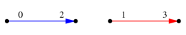
Figure 9: Mapping between $TTS$-labelings and transversal structures.

Figure 10 shows the TTS-labeling corresponding to the transversal structure of Figure 4. This labeling is also represented on the corresponding orientation of its angle map.

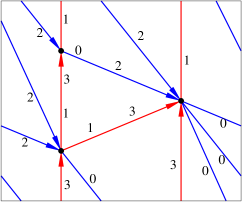
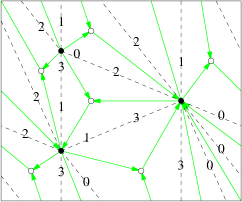
Figure 10: Labeling of the half-edges of a transversal structure and in the angle map.

We say that a 4-orientation of $A(G)$ admits a TTS-labeling if there is a labeling of the angles of the primal-vertices of $A(G)$ such that this labeling corresponds to a transversal structure of $G$ (as on Figure 10).

The goal of this section is to characterize which are the 4-orientations that admit TTS-labelings. For that purpose we have to introduce some more formalism, similarly to what is done for Schnyder woods (see [GKL16, Lév17]).

3.2 A bit of homology

We need a bit of surface homology of general maps which we discuss now.

Consider a map $G=(V,E)$, on an orientable surface of genus $g$, given with an arbitrary orientation of its edges. This fixed arbitrary orientation is implicit in all the paper and is used to handle flows. A flow $\phi$ on $G$ is a vector in $\mathbb{Z}^{E}$. For any $e\in E$, we denote by $\phi_{e}$ the coordinate $e$ of $\phi$.

A walk $W$ of $G$ is a sequence of edges with a direction of traversal such that the ending point of an edge is the starting point of the next edge. A walk is closed if the start and end vertices coincide. A walk has a characteristic flow $\phi(W)$ defined by:

$$\phi(W)_{e}=\#\text{times }W\text{ traverses }e\text{ forward}-\#\text{times }\\ W\text{ traverses }e\text{ backward}.$$

This definition naturally extends to sets of walks. From now on we consider that a set of walks and its characteristic flow are the same object and by abuse of notation we can write $W$ instead of $\phi(W)$. We do the same for oriented subgraphs, i.e., subgraphs that can be seen as a set of walks of unit length.

A facial walk is a closed walk bounding a face. Let $\mathcal{F}$ be the set of counterclockwise facial walks and let $\mathbb{F}={<}\phi(\mathcal{F}){>}$ be the subgroup of $\mathbb{Z}^{E}$ generated by $\mathcal{F}$. Two flows $\phi,\phi^{\prime}$ are homologous if $\phi-\phi^{\prime}\in\mathbb{F}$. They are weakly homologous if $\phi-\phi^{\prime}\in\mathbb{F}$ or $\phi+\phi^{\prime}\in\mathbb{F}$. We say that a flow $\phi$ is $0$-homologous if it is homologous to the zero flow, i.e. $\phi\in\mathbb{F}$.

Let $\mathcal{W}$ be the set of closed walks and let $\mathbb{W}={<}\phi(\mathcal{W}){>}$ be the subgroup of $\mathbb{Z}^{E}$ generated by $\mathcal{W}$. The group $H(G)=\mathbb{W}/\mathbb{F}$ is the first homology group of $G$. It is well-known that $H(G)$ only depends on the genus of the map, and actually it is isomorphic to $\mathbb{Z}^{2g}$.

A set $\{B_{1},\ldots,B_{2g}\}$ of (closed) walks of $G$ is said to be a basis for the homology if the equivalence classes of their characteristic vectors $([\phi(B_{1})],\ldots,[\phi(B_{2g})])$ generate $H(G)$. Then for any closed walk $W$ of $G$, we have $W=\sum_{F\in\mathcal{F}}\lambda_{F}F+\sum_{1\leq i\leq 2g}\mu_{i}B_{i}$ for some $\lambda\in\mathbb{Z}^{\mathcal{F}},\mu\in\mathbb{Z}^{2g}$. Moreover one of the $\lambda_{F}$ can be set to zero (and then all the other coefficients are unique).

For any map, there exists a set of cycles that forms a basis for the homology and it is computationally easy to build. A possible way to do this is by considering a spanning tree $T$ of $G$, and a spanning tree $T^{*}$ of $G^{*}$ that contains no edges dual to $T$. By Euler’s formula, there are exactly $2g$ edges in $G$ that are not in $T$ nor dual to edges of $T^{*}$. Each of these $2g$ edges forms a unique cycle with $T$. It is not hard to see that this set of cycles, given with any direction of traversal, forms a basis for the homology. Moreover, note that the intersection of any pair of these cycles is either a single vertex or a common path.

The edges of the dual map $G^{*}$ of $G$ are oriented such that the dual $e^{*}$ of an edge $e$ of $G$ goes from the face on the right of $e$ to the face on the left of $e$. Let $\mathcal{F}^{*}$ be the set of counterclockwise facial walks of $G^{*}$. Consider $\{B^{*}_{1},\ldots,B^{*}_{2g}\}$ a set of closed walks of $G^{*}$ that form a basis for the homology. Let $p$ and $d$ be flows of $G$ and $G^{*}$, respectively. We define the following:

$$\beta(p,d)=\sum_{e\in G}p_{e}d_{e^{*}}.$$

Note that $\beta$ is a bilinear function. We need the following lemma from [GKL16]:

Lemma 7 ([GKL16, Lemma 3.1])

Given two flows $\phi,\phi^{\prime}$ of $G$, the following properties are equivalent to each other:

1. The two flows $\phi,\phi^{\prime}$ are homologous.

2. For any closed walk $W$ of $G^{*}$ we have $\beta(\phi,W)=\beta(\phi^{\prime},W)$.

3. For any $F\in\mathcal{F^{*}}$, we have $\beta(\phi,F)=\beta(\phi^{\prime},F)$, and, for any $1\leq i\leq 2g$, we have $\beta(\phi,B^{*}_{i})=\beta(\phi^{\prime},B^{*}_{i})$.

3.3 The angle-dual-completion

Consider a toroidal triangulation $G$. The angle-dual-completion $\widehat{{A(G)}}$ of $G$ is the map obtained from simultaneously embedding $A(G)$ and $G^{*}$ and subdividing each edge of $G^{*}$ by adding a vertex at its intersection with the corresponding primal-edge of $G$ (see Figure 11). In $\widehat{{A(G)}}$ there are three types of vertices called primal-, dual- and edge-vertices, represented, respectively, in black, white, and gray on the figures. There are two types of edges called angle- and dual-edges. Each angle-edge is between a primal- and dual-vertex. Each dual-edge is between a dual- and an edge-vertex. Since $G$ is a triangulation, each dual-vertex is incident to three angle-edges and three dual-edges. Each edge-vertex is incident to two dual-edges. Each face of $\widehat{{A(G)}}$ represents a half-edge of $G$ and is a quadrangle incident to one primal-vertex, two dual-vertices and one edge-vertex.

Given an orientation of the angle map $A(G)$, this orientation naturally extends to an orientation of the angle-dual-completion $\widehat{{A(G)}}$ where angle-edges get the orientation they have in $A(G)$ and dual-edges are oriented from the edge-vertex to the dual-vertex. A 4-orientation of $\widehat{{A(G)}}$ is an orientation of its edges that corresponds to a 4-orientation of $A(G)$, i.e. primal-vertices have outdegree exactly $4$, dual-vertices have out-degree exactly $1$ and edge-vertices have outdegree exactly $2$.

A TTS-labeling of $G$ can be represented on $\widehat{{A(G)}}$ by putting labels into faces of $\widehat{{A(G)}}$ (see Figure 11). When crossing an angle-edge that is incoming for a primal-vertex, the label does not change. When crossing an angle-edge that is outgoing for a primal-vertex, the label changes by $\pm 1$ depending on the orientation of this angle-edge: from left to right $(+1\bmod 4)$ or right to left $(-1\bmod 4)$. When crossing a dual-edge the label changes by $\pm 2$, and the orientation is not relevant since $-2\bmod 4=+2\bmod 4$.

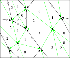
Figure 11: Orientation and labeling of the angle-dual-completion corresponding to Figure 10.

Let ${Out}$ be the set of edges of $\widehat{{A(G)}}$ which are going from a primal-vertex to a dual-vertex. We call these edges out-edges of $\widehat{{A(G)}}$. Let ${Dual}$ be the set of dual-edges of $\widehat{{A(G)}}$. For $\phi$ a flow of the dual of the angle-dual-completion $\widehat{{A(G)}}^{*}$, we define $\delta(\phi)=\beta({Out},\phi)+2\beta({Dual},\phi)$. More intuitively, if $W$ is a walk of $\widehat{{A(G)}}^{*}$, then:

$$\begin{array}[]{ll}\delta(W)=&\ \ \#\text{out-edges crossing }W\text{ from left to right}\\ &-\#\text{out-edges crossing }W\text{ from right to left}\\ &+\ 2\times\#\text{dual-edges crossing }W\text{ from left to right}\\ &-\ 2\times\#\text{dual-edges crossing }W\text{ from right to left}\\ \end{array}$$

The bilinearity of $\beta$ implies the linearity of $\delta$.

The following lemma gives a necessary and sufficient condition for a 4-orientation of the angle map to admit a TTS-labeling.

Lemma 8

A 4-orientation of ${A(G)}$ admits a TTS-labeling if and only if any closed walk $W$ of $\widehat{{A(G)}}^{*}$ satisfies $\delta(W)=0\bmod 4$.

Proof. $(\Longrightarrow)$ Consider a TTS-labeling $\ell$ of $A(G)$. The definition of $\delta$ is such that $\delta$ modulo $4$ counts the variation of the labels when going from one face of $\widehat{{A(G)}}$ to another face of $\widehat{{A(G)}}$. Thus for any walk $W$ of $\widehat{{A(G)}}^{*}$ from a face $F$ to a face $F^{\prime}$, the value of $\delta(W)\bmod 4$ is equal to $\ell(F^{\prime})-\ell(F)\bmod 4$. Thus if $W$ is a closed walk then $\delta(W)=0\bmod 4$.

$(\Longleftarrow)$ Consider a 4-orientation of $\widehat{{A(G)}}$ such that any closed walk $W$ of $\widehat{{A(G)}}^{*}$ satisfies $\delta(W)=0\bmod 4$. Pick any face $F_{0}$ of $\widehat{{A(G)}}$ and label it $0$. Consider any face $F$ of $\widehat{{A(G)}}$ and a path $P$ of $\widehat{{A(G)}}^{*}$ from $F_{0}$ to $F$. Label $F$ with the value $\delta(P)\bmod 4$. Note that the label of $F$ is independent from the choice of $P$ as for any two paths $P_{1},P_{2}$ going from $F_{0}$ to $F$, we have $\delta(P_{1})=\delta(P_{2})\bmod 4$ since $\delta(P_{1}-P_{2})=0\bmod 4$ as $P_{1}-P_{2}$ is a closed walk.

Consider a primal-vertex $v$ of $\widehat{{A(G)}}$. By assumption $d^{+}(v)=4$ so the labels around $v$ form in counterclockwise order four non-empty intervals of $0$, $1$, $2$, $3$. Moreover, the labels of the two faces incident to an edge-vertex differ by $(2\bmod 4)$. So the obtained labeling corresponds to a TTS-labeling of $G$. $\Box$

In the next section we study properties of $\delta$ w.r.t. homology in order to simplify the condition of Lemma 8 that concerns any closed walk of $\widehat{{A(G)}}^{*}$. We also replace the condition on $\delta$ to a condition on $\gamma$ that is simpler to handle.

3.4 Characterization theorem

Consider a toroidal triangulation $G$. Let $\widehat{\mathcal{F}^{*}}$ be the set of counterclockwise facial walks of the angle-dual-completion $\widehat{{A(G)}}^{*}$.

We have the following lemmas:

Lemma 9

In a $4$-orientation of $\widehat{{A(G)}}$, any $F\in\widehat{\mathcal{F}^{*}}$ satisfies $\delta(F)=0\bmod 4$.

Proof. If $F$ corresponds to a primal-vertex $v$ of $\widehat{{A(G)}}$, then $v$ has outdegree exactly $4$. So $\delta(F)=4=0\bmod 4$.

If $F$ corresponds to a dual-vertex $v$ of $\widehat{{A(G)}}$, then $v$ is incident to three angle-edges, exactly two of which are incoming (and thus in Out), and incident to three incoming dual-edges. So $\delta(F)=-2\times 1-3\times 2=-8=0\bmod 4$.

If $F$ corresponds to an edge-vertex $v$ of $\widehat{{A(G)}}$, then $v$ is incident to two outgoing dual-edges. So $\delta(F)=2\times 2=4=0\bmod 4$. $\Box$

Lemma 10

In a $4$-orientation of $\widehat{{A(G)}}$, if $\{B_{1},B_{2}\}$ is a pair of cycles of $\widehat{{A(G)}}^{*}$, given with a direction of traversal, that forms a basis for the homology, then for any closed walk $W$ of $\widehat{{A(G)}}^{*}$ homologous to $\mu_{1}B_{1}+\mu_{2}B_{2}$, $\mu\in\mathbb{Z}^{2}$ we have $\delta(W)=\mu_{1}\delta(B_{1})+\mu_{2}\delta(B_{2})\bmod 4$.

Proof. We have $W=\sum_{F\in\widehat{\mathcal{F}^{*}}}\lambda_{F}F+\mu_{1}B_{1}+\mu_{2}B_{2}$ for some $\lambda\in\mathbb{Z}^{f}$, $\mu\in\mathbb{Z}^{2}$. Then by linearity of $\delta$ and Lemma 9, the lemma follows. $\Box$

Lemma 10 can be used to simplify the condition of Lemma 8 and show that if $\{B_{1},B_{2}\}$ is a pair of cycles of $\widehat{{A(G)}}^{*}$ that forms a basis for the homology, then a $4$-orientation of $\widehat{{A(G)}}$ admits a TTS-labeling if and only if $\delta(B_{i})=0\bmod 4$, for $i\in\{1,2\}$. We prefer to formulate such a result with function $\gamma$ that is simpler to handle (see Theorem 1).

Let $C$ be a cycle of $G$ with a direction of traversal. Let $W_{L}(C)$ be the closed walk of $\widehat{{A(G)}}^{*}$ just on the left of $C$ and going in the same direction as $C$. Note that since the faces of $\widehat{{A(G)}}^{*}$ have exactly one incident vertex that is a primal-vertex, the walk $W_{L}(C)$ is in fact a cycle of $\widehat{{A(G)}}^{*}$. Similarly, let $W_{R}(C)$ be the cycle of $\widehat{{A(G)}}^{*}$ just on the right of $C$ and going in the same direction as $C$.

Lemma 11

Consider a $4$-orientation of ${A(G)}$ and a cycle $C$ of $G$, then we have:

$$\gamma(C)=\delta(W_{L}(C))+\delta(W_{R}(C))$$

$$\delta(W_{L}(C))=0\bmod 4\iff\gamma(C)=0\bmod 8.$$

Proof. Let $x_{R}$ (resp. $x_{L}$) be the number of edges of $A(G)$ leaving $C$ on its right (resp. left). So $\gamma(C)=x_{R}-x_{L}$. Let $k$ be the number of vertices of $C$. Since we are considering a $4$-orientation of $A(G)$, we have $x_{R}+x_{L}=4k$. Moreover, an edge of $A(G)$ leaving $C$ on its right (resp. left) is counting $+1$ (resp. $-1$) for $\delta(W_{R}(C))$ (resp. $\delta(W_{L}(C))$). For each edge of $C$ there is a corresponding edge-vertex in $\widehat{{A(G)}}$, that is incident to two dual-edges of $\widehat{{A(G)}}$, one that is crossing $\delta(W_{L}(C))$ from right to left, counting $-2$, and one crossing $\delta(W_{R}(C))$ from left to right, counting $+2$. So $\delta(W_{L}(C))=-2k-x_{L}$ and $\delta(W_{R}(C))=2k+x_{R}$.

Combining these equalities, one obtain: $\gamma(C)=\delta(W_{L}(C))+\delta(W_{R}(C))$, $\gamma(C)=2\delta(W_{L}(C))+8k$, $\delta(W_{L}(C))=\gamma(C)/2-4k$. Then clearly, $\delta(W_{L}(C))=0\bmod 4$ implies $\gamma(C)=0\bmod 8$, and $\gamma(C)=0\bmod 8$ implies $\delta(W_{L}(C))=0\bmod 4$. $\Box$

Finally, we have the following theorem which characterizes the 4-orientations that admit TTS-labelings:

Theorem 1

Consider a toroidal triangulation $G$. Let $\{B_{1},B_{2}\}$ be a pair of cycles of $G$, given with a direction of traversal, that forms a basis for the homology. A $4$-orientation of $A(G)$ admits a toroidal transversal structure labeling if and only if $\gamma(B_{1})=0\bmod 8$ and $\gamma(B_{2})=0\bmod 8$.

Proof. $(\Longrightarrow)$ By Lemma 8, we have $\delta(W)=0\bmod 4$ for any closed walk $W$ of $\widehat{{A(G)}}^{*}$. So we have $\delta(W_{L}(B_{1})),\delta(W_{L}(B_{2}))$, are both equal to $0\bmod 4$. Thus, by Lemma 11, we have $\gamma(B_{i})=0\bmod 8$, for $i\in\{1,2\}$.

$(\Longleftarrow)$ Suppose that $\gamma(B_{i})=0\bmod 4$, for $i\in\{1,2\}$. By Lemma 11, we have $\delta(W_{L}(B_{i}))=0\bmod 4$, for $i\in\{1,2\}$. Moreover $\{W_{L}(B_{1}),W_{L}(B_{2})\}$ forms a basis for the homology. So by Lemma 10, $\delta(W)=0\bmod 4$ for any closed walk $W$ of $\widehat{{A(G)}}^{*}$. So the orientation admits a TTS-labeling by Lemma 8. $\Box$

The $4$-orientation of the toroidal triangulation on the left of Figure 2 is an example where some non-contractible cycles have value $\gamma$ not equal to $0\bmod 8$. The vertical loop of the triangulation, with upward direction of traversal, has $\gamma=2$. Thus by Theorem 1, this orientation does not correspond to a transversal structure. Whereas, on the right example, one can check that $\gamma=0$ for a vertical cycle and a horizontal one, thus this orientation corresponds to a transversal structure (represented on Figure 4).

A consequence of Theorem 1 is that any balanced 4-orientation of the angle graph $A(G)$ of a toroidal triangulation $G$ admits a TTS-labeling and thus is the $4$-orientation corresponding to a transversal structure of $G$.

Corollary 1

Any balanced 4-orientation of $A(G)$ is the $4$-orientation corresponding to a (balanced) transversal structure of $G$.

Note again that there are transversal structures whose corresponding 4-orientations are not balanced, thus for which $\gamma=0\bmod 8$ for every non-contractible cycles, but not exactly $0$ for some of them. Such an example is given on Figure 7.

4 Existence of balanced transversal structures

In this section we prove existence of balanced transversal structures for essentially 4-connected triangulations by contracting edges until we obtain a triangulation with just one vertex. This is done by preserving the property that the triangulation is essentially 4-connected. The toroidal triangulation on one vertex is represented on Figure 12 with a balanced transversal structure and the corresponding angle map. Then the graph can be decontracted step by step to obtain a balanced transversal structures of the original triangulation.

Figure 12: Example of a balanced transversal structure of the toroidal triangulation on one vertex.

4.1 Contraction preserving “essentially 4-connected”

Given a toroidal triangulation $G$, the contraction of a non-loop-edge $e$ of $G$ is the operation consisting of continuously contracting $e$ until merging its two ends. We note $G/e$ the obtained map. On Figure 13 the contraction of an edge $e$ is represented. Note that only one edge of each multiple edges that is created is preserved (edge $e_{wx}$ and $e_{wy}$ on the figure).

$G$		$G/e$

Figure 13: The contraction operation for triangulations

Note that the contraction operation is also defined when some vertices are identified: $x=u$ and $y=v$ (the case represented on Figure 14), or $x=v$ and $y=u$ (corresponding to the symmetric case with a diagonal in the other direction).

$G$		$G/e$

Figure 14: The contraction operation when some vertices are identified.

In [Moh96] it is proved that in a toroidal triangulation (with no contractible loop nor homotopic multiple edges) with at least two vertices, one can find an edge whose contraction preserves the fact that the map is a toroidal triangulation (with no contractible loop nor homotopic multiple edges). Here we also need to show that we can preserve the fact of being essentially 4-connected during contraction. We say that a non-loop edge $e$ of an essentially 4-connected toroidal triangulation $G$ is contractible if $G/e$ is an essentially 4-connected toroidal triangulation. We have the following lemma:

Lemma 12

An essentially 4-connected toroidal triangulation with at least two vertices has a contractible edge.

Proof. For $k\geq 3$, a separating k-walk is a closed walk of size $k$ that delimits on one side a region homeomorphic to an open disk containing at least one vertex. This region is called the interior of the separating k-walk. A separating $3$-walk is a separating triangle and we call a separating $4$-walk a separating quadrangle.

Let $G$ be an essentially 4-connected toroidal triangulation with at least two vertices. By Lemma 5, the map $G$ has no contractible loop, no homotopic multiple edges and no separating triangle. Consider a non-loop edge $e$ of $G$. The contracted graph $G/e$ is an essentially 4-connected toroidal triangulation if and only if $G/e$ has no contractible loop, no homotopic multiple edges and no separating triangle.

Since $G$ has no homotopic multiple edges, the contraction of $e$ cannot create a contractible loop. Since $G$ has no separating triangle, the only way to create a pair of homotopic multiple edges in $G/e$ is if $e$ appears twice on a separating quadrangle such that each extremity of $e$ is incident to a non-contractible loop as depicted on Figure 15.a (where the dashed region represents the interior of the separating quadrangle). There are two ways to create a separating triangle in $G/e$: either $e$ appears once on a separating quadrangle as depicted on Figure 15.b, where some vertices may be identified but not edges, or $e$ appears twice on a separating 5-walk such that one extremity of $e$ is incident to a non-contractible loop and the other extremity is incident to edges distinct from $e$ forming a non-contractible cycle of size two as depicted on Figure 15.c.

Case a
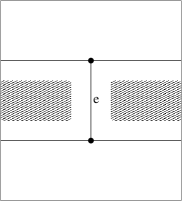
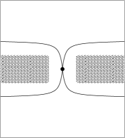
Case b
Case c
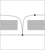
	$G$		$G/e$

Figure 15: Contraction of an edge $e$ creating a pair of homotopic multiple edges or a separating triangle.

We consider two cases whether there are separating quadrangles in $G$ or not.

• $G$ has some separating quadrangles:

  An inner chord of a separating quadrangle $Q$ is an edge between its vertices that lie in the interior of the separating quadrangle. We claim that a separating quadrangle $Q$ of $G$ has no inner chord. Suppose by contradiction that such a chord exists. Since there is no pair of homotopic multiple edges, this chord is between “opposite” vertices of $Q$. Thus it partitions the interior of $Q$ into two triangles. These two triangles are not separating by assumption on $G$ and thus the quadrangle $Q$ is not separating either, a contradiction.

  Let $Q$ be a maximal separating quadrangle. Suppose by contradiction that there exists a separating quadrangle $Q^{\prime}$ of $G$ distinct from $Q$ whose interior $R^{\prime}$ intersects $R$ and is not included in $R$. By maximality of $Q$, we also have $R$ is not included in $R^{\prime}$. As observed previously, $Q$ and $Q^{\prime}$ have no inner chord. So there is at least one or two vertices of $Q$ (resp $Q^{\prime}$) in the interior of $Q^{\prime}$ (resp. $Q$). Thus the border of the union of $R$ and $R^{\prime}$ has size less or equal to four, a contradiction to the maximality of $Q$ or of $G$ being an essentially $4$-connected triangulation. So a separating quadrangle of $G$ whose interior intersects $R$ has its interior included in $R$.

  Let $G^{\prime}$ be the map obtained from $G$ by keeping all the vertices and edges in $R$, including $Q$. The vertices and edges appearing several times on $Q$ are duplicated so $G^{\prime}$ is a planar map. Then $G^{\prime}$ is a 4-connected planar map in which every inner face is a triangle and the outer face is a quadrangle. Let $a,b,c,d$ denote the outer vertices of $G^{\prime}$ in counterclockwise order. We denote also $a,b,c,d$ the corresponding vertices of $G$. Note that in $G$ some of these vertices might be identified. We consider two cases, whether, in $G^{\prime}$, there exists an inner vertex incident to at least three outer vertices or not.

  • In $G^{\prime}$, there exists an inner vertex $v$ that is incident to at least three outer vertices:

    W.l.o.g., we may assume that $v$ is incident to $a,b,c$ in $G^{\prime}$ with edges $e_{a},e_{b},e_{c}$ respectively. We prove that $e_{b}$ is contractible in $G$.

    Suppose by contradiction that $e_{b}$ belongs to a separating quadrangle $Q^{\prime}$ of $G$. Then $Q^{\prime}$ is distinct from $Q$ and its interior $R^{\prime}$ of $Q^{\prime}$ intersects $R$. Thus by the above remark, $R^{\prime}$ is included in $R$. Then $Q^{\prime}$ has an inner chord $e_{a}$ or $e_{c}$, a contradiction.

    Suppose that $e_{b}$ appears twice on a separating 5-walk $W$ as depicted on Figure 15.c. Then, one of the extremity of $e_{b}$ is incident to a non-contractible loop $\ell$ of $W$ and this extremity cannot lie inside $R$ so it is $b$. So $v$ is incident to two edges $e_{1},e_{2}$, distinct from $e_{b}$, so that the 5-walk $W$ is the sequence of edges $\ell,e_{b},e_{1},e_{2},e_{b}$. Then, in $G^{\prime}$, the edges $e_{1},e_{2}$ are incident to two distinct vertices of $\{a,c,d\}$ that are identified in $G$ so that $e_{1},e_{2}$ form a non-contractible cycle of size two of $G$.

    Suppose, by contradiction, that $e_{1},e_{2}$ are incident to “consecutive” vertices of $Q$, then w.l.o.g., we can assume that $e_{1},e_{2}$ are incident to $a$ and $d$ that are identified in $G$. If $b,c$ are also identified in $G$, then we are in the situation of Figure 16.a, with $W$ represented in magenta. Then, the interior of the separating 5-walk $W$ is partitioned into triangles whose interiors are empty since $G$ is essentially 4-connected. So the interior of the separating 5-walk $W$ contains no vertices, a contradiction. If $b,c$ are not identified, then we are in the situation of Figure 16.b. Then the two loops of the figure plus $e$ form a quadrangle whose interior strictly contains the interior of $Q$, a contradiction to the maximality of $Q$.

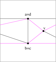
    Case a	Case b	Case c

    Figure 16: Cases of Lemma 12.

    So, $e_{1},e_{2}$ are incident to “opposite” vertices of $Q$. These two vertices are $a$ and $c$ and they are identified in $G$. Then we are in the situation of Figure 16.c . Then, the interior of the separating 5-walk $W$ is partitioned into triangles whose interior are empty since $G$ is essentially 4-connected. So the interior of the separating 5-walk $W$ contains no vertices, a contradiction.

    To conclude, $e_{b}$ does not belong to a separating quadrangle, nor appears twice on a separating 5-walk, so $e_{b}$ is contractible in $G$.

  • In $G^{\prime}$, all inner vertices are incident to at most two outer vertices:

    Kant and He proved [KH97, Lemma 3.1] that $G^{\prime}$ contains an internal edge $e$ such that $G^{\prime}/e$ is 4-connected. Let us show $e$ is contractible in $G$.

    Suppose by contradiction that $e$ belongs to a separating quadrangle $Q^{\prime}$ of $G$. Then the interior $R^{\prime}$ of $Q^{\prime}$ intersects $R$ and thus is included in $R$ by above remark. But then $G^{\prime}/e$ is not 4-connected, a contradiction.

    Suppose by contradiction that $e^{\prime}$ appears twice on a separating 5-walk as depicted on Figure 15.c. Then, in $G$, one extremity $u$ of $e^{\prime}$ is incident to a non-contractible loop and the other extremity $v$ of $e^{\prime}$ is incident to two edges $e_{1},e_{2}$, distinct from $e^{\prime}$, forming a non-contractible cycle of size two. Thus $u$ is not an inner vertex of $G^{\prime}$ and the two extremities of $e_{1},e_{2}$ also. So $v$ is incident to three outer vertices of $G^{\prime}$, a contradiction.

    To conclude, $e$ does not belong to a separating quadrangle, nor appears twice on a separating 5-walk, so $e$ is contractible in $G$.

• $G$ has no separating quadrangle:

  Consider a non-loop edge $e$ of $G$. If $e$ is contractible we are done, so we can assume that $e$ is not contractible. Then, since there is no separating quadrangle, we have $e$ that appears twice on a separating 5-walk $W$ as depicted on Figure 15.c. More precisely, one extremity $u$ of $e$ is incident to a non-contractible loop $\ell$ and the other extremity $v$ of $e$ is incident to two edges $e_{1},e_{2}$, distinct from $e$, forming a non-contractible cycle of size two of $G$. Let $R$ be the interior of the separating 5-walk $W$. We consider two cases whether $v$ has some neighbors in the strict interior of $R$ or not.

  Suppose by contradiction that $v$ has no neighbors in the strict interior of $R$. Then either $v$ has some incident edges inside $R$ or not. Suppose first that $v$ has some incident edges inside $R$. Then, since $v$ has no neighbors in the strict interior of $R$, we have that $v$ is incident to $u$ with an edge in the strict interior of $R$, as depicted on Figure 17.a. Then since there is no separating triangle, nor separating quadrangle, the region $R$ contains no vertices, a contradiction. Suppose now that $v$ has no incident edge inside $R$. Then, Since $G$ is a triangulation, vertex $u$ must be incident twice to the third vertex $w$ of the $5$-walk $w$, as depicted on Figure 17.b. Again since there is no separating triangle, the region $R$ contains no vertices, a contradiction.

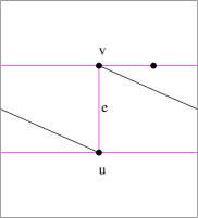
  Case a	Case b	Case c

  Figure 17: Cases of Lemma 12.

  So $v$ has a neighbor $x$ in the strict interior of $R$. Let $e^{\prime}$ be the edge between $v,x$. If $e^{\prime}$ appears twice on a separating 5-walk $W$, then $x$ is incident twice to $u$ to form a non-contractible cycle of size two and $v$ is incident to a non-contractible loop $\ell^{\prime}$, as depicted on Figure 17.c. Then $e,\ell,\ell^{\prime}$ forms a separating quadrangle, a contradiction. So $e^{\prime}$ is contractible.

$\Box$

4.2 Balanced properties and homology

In Section 3, we have proved some properties of $\gamma$ (or $\delta$) w.r.t. homology. The obtained equalities where conditioned by a “modulo”. In next lemma we prove some properties of $\gamma$ w.r.t. a basis for the homology with exact equality to obtain a simple condition to prove that a $4$-orientation is balanced (see Lemma 14).

Consider an essentially 4-connected toroidal triangulation $G$ and its angle map $A(G)$.

Lemma 13

Consider a $4$-orientation of $A(G)$, a non-contractible cycle $C$ of $G$, given with a direction of traversal, and a basis for the homology $\{B_{1},B_{2}\}$ of $G$, such that $B_{1},B_{2}$ are non-contractible cycles whose intersection is a single vertex or a common path. If $C$ is homologous to $k_{1}B_{1}+k_{2}B_{2}$, then $\gamma(C)=k_{1}\,\gamma(B_{1})+k_{2}\,\gamma(B_{2})$.

Proof. Let $v$ be a vertex in the intersection of $B_{1},B_{2}$ such that, if this intersection is a common path, then $v$ is one of the extremities of this path and let $u$ be the other extremity. Consider a drawing of ${G}^{\infty}$ obtained by replicating a flat representation of ${G}$ to tile the plane. Let $v_{0}$ be a copy of $v$ in ${G}^{\infty}$. Consider the walk $W$ starting from $v_{0}$ and following $k_{1}$ times the edges corresponding to $B_{1}$ and then $k_{2}$ times the edges corresponding to $B_{2}$ (we are going backward if $k_{i}$ is negative). This walk ends at a copy $v_{1}$ of $v$. Since $C$ is non-contractible we have $k_{1}$ or $k_{2}$ not equal to $0$ and thus $v_{1}$ is distinct from $v_{0}$. Let $W^{\infty}$ be the infinite walk obtained by replicating $W$ (forward and backward) from $v_{0}$. Note that there might be some repetition of vertices in $W^{\infty}$ if the intersection of $B_{1},B_{2}$ is a path. But in that case, by the choice of $B_{1},B_{2}$ (i.e. whose intersection is a single vertex or a common path), we have that $W^{\infty}$ is almost a path, except maybe at all the transitions from “$k_{1}{B_{1}}$” to “$k_{2}B_{2}$”, or at all the transitions from “$k_{2}{B_{2}}$” to “$k_{1}B_{1}$”, where it can go back and forth a path corresponding to the intersection of $B_{1}$ and $B_{2}$. The existence or not of such “back and forth” parts depends on the signs of $k_{1},k_{2}$ and the way $B_{1},B_{2}$ are going through their common path. Figure 19 gives an example of this construction with $(k_{1},k_{2})=(1,1)$ and $(k_{1},k_{2})=(1,-1)$ when $B_{1},B_{2}$ intersects on a path and are oriented the same way along this path as on Figure 18.

Figure 18: Intersection of the basis.

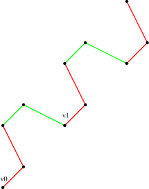
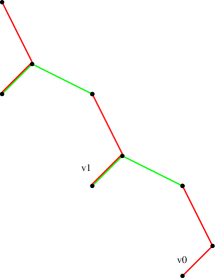
$(k_{1},k_{2})=(1,1)$	$(k_{1},k_{2})=(1,-1)$

Figure 19: Replicating “$k_{1}{B_{1}}$” and “$k_{2}B_{2}$” in the universal cover.

We “simplify” $W^{\infty}$ by removing all the parts that consists of going back and forth along a path (if any) and call $B^{\infty}$ the obtained walk that is now without repetition of vertices. By the choice of $v$, we have that $B^{\infty}$ goes through copies of $v$. If $v_{0},v_{1}$ are no more a vertex along $B^{\infty}$, because of a simplification at the transition from “$k_{2}{B_{2}}$” to “$k_{1}B_{1}$”, then we replace $v_{0}$ and $v_{1}$ by the next copies of $v$ along $W^{\infty}$, i.e. at the transition from “$k_{1}{B_{1}}$” to “$k_{2}B_{2}$”.

Since ${C}$ is homologous to $k_{1}{B_{1}}+k_{2}{B_{2}}$, we can find an infinite path $C^{\infty}$, that corresponds to copies of $C$ replicated, that does not intersect $B^{\infty}$ and situated on the right side of $B^{\infty}$. Now we can find a copy $B^{\prime\infty}$ of $B^{\infty}$, such that $C^{\infty}$ lies between $B^{\infty}$ and $B^{\prime\infty}$ without intersecting them. Choose two copies $v^{\prime}_{0},v^{\prime}_{1}$ of $v_{0},v_{1}$ on $B^{\prime\infty}$ such that the vectors $v_{0}v_{1}$ and $v^{\prime}_{0}v^{\prime}_{1}$ are equal.

Let $R_{0}$ be the region bounded by $B^{\infty},B^{\prime\infty}$. Let $R_{1}$ (resp. $R_{2}$) be the subregion of $R_{0}$ delimited by $B^{\infty}$ and $C^{\infty}$ (resp. by $C^{\infty}$ and $B^{\prime\infty}$). We consider $R_{0},R_{1},R_{2}$ as cylinders, where part of the lines $(v_{0},v^{\prime}_{0}),(v_{1},v_{1}^{\prime})$ are identified. Let $B,B^{\prime},C^{\prime}$ be the cycles of $R_{0}$ corresponding to $B^{\infty},B^{\prime\infty},C^{\infty}$ respectively.

Let $x$ (resp. $y$) be the number of edges of $A(G)^{\infty}$ leaving $B$ (resp. $B^{\prime}$) in $R_{0}$. Let $x^{\prime}$ (resp. $y^{\prime}$) be the number of edges of $A(G)^{\infty}$ leaving $C^{\prime}$ on its right (resp. left) side in $R_{0}$. We have $C^{\prime}$ corresponds to exactly one copy of $C$, so $\gamma(C)=x^{\prime}-y^{\prime}$. Similarly, we have $B$ and $B^{\prime}$ that almost corresponds to $k_{1}$ copies of $B_{1}$ followed by $k_{2}$ copies of $B_{2}$, except the fact that we may have removed a back and forth part (if any). In any case we have the following:

Claim 1

$k_{1}\,\gamma(B_{1})+k_{2}\,\gamma(B_{2})=x-y$

Proof.  We prove the case where the common intersection of $B_{1},B_{2}$ is a path (if the intersection is a single vertex, the proof is even simpler). We assume, w.l.o.g, by eventually reversing one of $B_{1}$ or $B_{2}$, that $B_{1},B_{2}$ are oriented the same way along their intersection, so we are in the situation of Figure 18.

Figure 20 shows how to compute $k_{1}\,\gamma(B_{1})+k_{2}\,\gamma(B_{2})+y-x$ when $(k_{1},k_{2})=(1,1)$. Then, one can check that each outgoing edge of the angle graph is counted exactly the same number of time positively and negatively. So everything compensates and we obtain $k_{1}\,\gamma(B_{1})+k_{2}\,\gamma(B_{2})+y-x=0$.

$\gamma(B_{1})$	$+$	$\gamma(B_{2})$	$+$	$(y-x)$	$=0$

Figure 20: Case $(k_{1},k_{2})=(1,1)$.

Figure 21 shows how to compute $k_{1}\,\gamma(B_{1})+k_{2}\,\gamma(B_{2})+y-x$ when $(k_{1},k_{2})=(1,-1)$. As above, most of the things compensate but, in the end, we obtain $k_{1}\,\gamma(B_{1})+k_{2}\,\gamma(B_{2})+y-x=d_{A(G)}^{+}(u)-d_{A(G)}^{+}(v)$, as depicted on the figure. Since the number of outgoing edges of $A(G)$ around each vertex is equal to $4$, we have again the conclusion $k_{1}\,\gamma(B_{1})+k_{2}\,\gamma(B_{2})+y-x=0$.

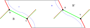
$\gamma(B_{1})$	$+$	$(-\gamma(B_{2}))$	$+$	$(y-x)$

$=d_{A(G)}^{+}(u)-d_{A(G)}^{+}(v)=0$

Figure 21: Case $(k_{1},k_{2})=(1,-1)$.

One can easily be convinced that when $|k_{1}|\geq 1$ and $|k_{2}|\geq 1$ then the same arguments apply. The only difference is that the red or green part of the figures in the universal cover would be longer (with repetitions of $B_{1}$ and $B_{2}$). This parts being very “clean”, they do not affect the way we compute the equality. Finally, if one of $k_{1}$ or $k_{2}$ is equal to zero, the analysis is simpler and the conclusion still holds. $\Diamond$

For $i\in\{1,2\}$, let $H_{i}$ be the cylinder map made of all the vertices and edges of ${G}^{\infty}$ that are in the cylinder region $R_{i}$. Let $k$ (resp. $k^{\prime}$) be the length of $B$ (resp. $C^{\prime}$). Let $n_{1},m_{1},f_{1}$ be respectively the number of vertices, edges and faces of $H_{1}$.

The number of edges of $A(G)^{\infty}$ in $H_{1}$ is equal to $3f_{1}$. Since we are considering a $4$-orientation of $A(G)$, these edges are decomposed into: the outgoing edges from inner vertices of $H_{1}$ (primal-vertices have outdegree $4$ in $A(G)^{\infty}$, so there are $4(n_{1}-k-k^{\prime})$ such edges), the outgoing edges from outer vertices of $H_{1}$ (there are $x+y^{\prime}$ such edges), and the outgoing edges from faces of $H_{1}$ (faces have outdegree $1$ in $A(G)^{\infty}$, so there are $f_{1}$ such edges). Finally, we have $3f_{1}=4(n_{1}-k-k^{\prime})+x+y^{\prime}+f_{1}$. Combining this with Euler’s formula, $n_{1}-m_{1}+f_{1}=0$, and the fact that all the faces of $H_{1}$ are triangles, i.e. $2m_{1}=3f_{1}+k+k^{\prime}$, one obtains that $x+y^{\prime}=2(k+k^{\prime})$. Similarly, by considering $H_{2}$, one obtain that $x^{\prime}+y=2(k+k^{\prime})$. Thus finally $x+y^{\prime}=x^{\prime}+y$ and thus $\gamma(C)=k_{1}\,\gamma(B_{1})+k_{2}\,\gamma(B_{2})$ by Claim 1. $\Box$

Lemma 13 implies the following:

Lemma 14

In a 4-orientation of $A(G)$, if for two non-contractible not weakly homologous cycles $C,C^{\prime}$ of ${G}$, we have $\gamma(C)=\gamma(C^{\prime})=0$, then the $4$-orientation of $A(G)$ is balanced.

Proof. Consider two non-contractible not weakly homologous cycles $C,C^{\prime}$ of ${G}$ such that $\gamma(C)=\gamma(C^{\prime})=0$. Consider an homology-basis $\{B_{1},B_{2}\}$ of $G$, such that $B_{1},B_{2}$ are non-contractible cycles whose intersection is a single vertex or a path (see Section 3.2 for discussion on existence of such a basis). Let $k_{1},k_{2},k^{\prime}_{1},k^{\prime}_{2}\in\mathbb{Z}$, such that $C$ (resp. $C^{\prime}$) is homologous to $k_{1}B_{1}+k_{2}B_{2}$ (resp. $k^{\prime}_{1}B_{1}+k^{\prime}_{2}B_{2}$). Since $C$ is non-contractible we have $(k_{1},k_{2})\neq(0,0)$. By eventually exchanging $B_{1},B_{2}$, we can assume, w.l.o.g., that $k_{1}\neq 0$. By Lemma 13, we have $k_{1}\gamma(B_{1})+k_{2}\gamma(B_{2})=\gamma(C)=0=\gamma(C^{\prime})=k^{\prime}_{1}\gamma(B_{1})+k^{\prime}_{2}\gamma(B_{2})$. So $\gamma(B_{1})=(-k_{2}/k_{1})\gamma(B_{2})$ and thus $(-k_{2}k^{\prime}_{1}/k_{1}+k^{\prime}_{2})\gamma(B_{2})=0$. So $k^{\prime}_{2}=k_{2}k^{\prime}_{1}/k_{1}$ or $\gamma(B_{2})=0$. Suppose by contradiction, that $\gamma(B_{2})\neq 0$. Then $(k^{\prime}_{1},k^{\prime}_{2})=\frac{k^{\prime}_{1}}{k_{1}}(k_{1},k_{2})$, and $C^{\prime}$ is homologous to $\frac{k^{\prime}_{1}}{k_{1}}C$. Since $C$ and $C^{\prime}$ are both non-contractible cycles, it is not possible that one is homologous to a multiple of the other, with a multiple different from $-1,1$. So $C,C^{\prime}$ are weakly homologous, a contradiction. So $\gamma(B_{2})=0$ and thus $\gamma(B_{1})=0$. Then by Lemma 13, any non-contractible cycle of ${G}$, have $\gamma$ equal to $0$. Thus the $4$-orientation is balanced $\Box$

4.3 Decontraction preserving “balanced”

The goal of this section is to prove the following lemma:

Lemma 15

If $G$ is a toroidal triangulation given with a non-loop edge $e$ whose extremities are of degree at least four and such that $G/e$ admits a balanced transversal structure, then $G$ admits a balanced transversal structure.

Proof. Let $G^{\prime}=G/e$ and consider a balanced transversal structure $G^{\prime}$. We show how to extend the balanced transversal structure of $G^{\prime}$ to a balanced transversal structure of $G$. Let $u,v$ be the two extremities of $e$ and $x,y$ the two vertices of $G$ such that the two faces incident to $e$ are $A=u,v,x$ and $B=v,u,y$ in clockwise order (see Figure 13). Note that $u$ and $v$ are distinct by definition of edge contraction but that $x$ and $y$ are not necessarily distinct, nor distinct from $u$ and $v$. Let $w$ be the vertex of $G^{\prime}$ resulting from the contraction of $e$. Let $e_{wx},e_{wy}$ be the two edges of $G^{\prime}$ represented on Figure 13 (these edges are identified and form a loop on Figure 14).

There are different cases to consider, corresponding to the different possible orientations and colorings of the edges $e_{wx}$ and $e_{wy}$ in $G^{\prime}$. By symmetry, there are just three cases to consider for Figure 13: edges $e_{wx}$ and $e_{wy}$ may be in consecutive, same or opposite intervals, w.r.t. the four intervals of the local property around $w$. When $e_{wx},e_{wy}$ are identified as in Figure 14, these “two” edges are necessarily in opposite intervals, and there is just one case to consider. So only the four cases represented on the left side of Figure 22 by case $x.0$ for $x\in\{a,b,c,d\}$ have to be considered.

a.0	a.1	a.2
b.0	b.1	b.2
c.0	c.1
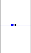
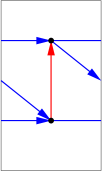
d.0	d.1

Figure 22: Decontraction rules of the transversal structure.

In each case $x.0$, we prove that one can color and orient the edges of $G$ to obtain a balanced transversal structure of $G$. For that purpose, just the edges of $G$ that are labeled on Figures 13 and 14 have to be specified, all the other edges of $G$ keep the orientation and coloring that they have in the balanced transversal structure of $G^{\prime}$. For each case $x.0$, with $x\in\{a,b,c,d\}$, the orientation and coloring of the labeled edges of $G$ are represented on the right side of Figure 22 by case $x.i$, $i\geq 1$. For the first two cases $x\in\{a,b\}$, we might have to choose between cases $x.1$ and $x.2$, to orient and color $G$, depending on a case analysis explained below. For the other cases, $x\in\{c,d\}$, there is just one coloring and orientation of $G$ to consider: case $x.1$.

The sector $]e_{1},e_{2}[$ of a vertex $w$, for $e_{1}$ and $e_{2}$ two edges incident to $w$, is the counterclockwise sector of $w$ between $e_{1}$ and $e_{2}$, excluding the edges $e_{1}$ and $e_{2}$.

Let us consider the different possible orientations and colorings of edges $e_{wx}$ and $e_{wy}$.

• $e_{wx}$ and $e_{wy}$ are not identified and in consecutive intervals:

  W.l.o.g., we might assume that we are in case a.0 of Figure 22, i.e. $e_{wx}$ (resp. $e_{wy}$) is a blue (resp. red) edge entering $w$.

  Since all vertices of $G$ have degree at least $4$, we have that $v$ is incident to at least one edge in the sector $]e_{vx},e_{vy}[$ of $v$. So $w$ is incident to at least one edge in the sector $]e_{wx},e_{wy}[$ of $w$. Such an edge can be blue or red in the transversal structure of $G^{\prime}$. Depending on if there is such a blue or red edge we apply coloring a.1 or a.2 to $G$, as explain below.

  W.l.o.g., we can assume that there is a blue edge incident to $w$ in the sector $]e_{wx},e_{wy}[$. By the local rule, this edge is entering $w$. Moreover the edge incident to $x$ and just after $e_{wx}$ in clockwise order around $x$ is entering $x$ in color red. So we are in the situation depicted on the left of Figure 23. Apply the coloring a.1 to $G$ as depicted on the right of Figure 23. One can easily check that the local property is satisfied around every vertex of $G$ (for that purpose one just as to check the local property around $u,v,x,y$). Thus we obtain a transversal structure of $G$.

  

  

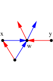
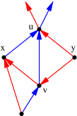
  Figure 23: Decontraction of case a.0 when there is a blue edge entering $w$ by below.

  It remains to prove that the obtained transversal structure is balanced. For that purpose consider two non-contractible not weakly homologous cycles $(B^{\prime}_{1},B^{\prime}_{2})$ of $G^{\prime}$. Since the transversal structure of $G^{\prime}$ is balanced, we have $\gamma(B^{\prime}_{1})=\gamma(B^{\prime}_{2})=0$ by definition of balanced property. If $B^{\prime}_{i}$ does not intersect $w$, then it is not affected by the decontraction, let $B_{i}=B^{\prime}_{i}$, so that $B_{i}$ is a cycle of $G$ with same homology and same value $\gamma$ as $B^{\prime}_{i}$. If $B^{\prime}_{i}$ intersects $w$, then one can consider where $B^{\prime}_{i}$ is entering and leaving the contracted region and replace $B^{\prime}_{i}$ by a cycle $B_{i}$ of $G$ with the same homology and same value $\gamma$ as $B^{\prime}_{i}$. This property illustrated on Figure 24, on the left part we consider an example of a cycle $B^{\prime}_{i}$ and on the right part we give a corresponding cycle $B_{i}$ having the same homology and $\gamma$ as $B^{\prime}_{i}$. To be completely convinced that this transformation works, one may consider all the different possibility to enter and leave the contracted region and check that one can find a corresponding cycle of $G$ with same $\gamma$. Finally, by this method, we obtain two non-contractible not weakly homologous cycles $B_{1},B_{2}$ of $G$ with $\gamma(B_{1})=\gamma(B_{2})=0$, so by Lemma 14, the obtained transversal structure is balanced.

  

  

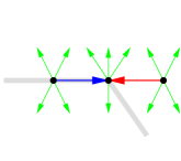
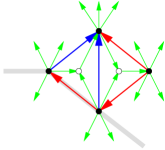
  Figure 24: Decontraction of case a.0 preserving $\gamma$.

• $e_{wx}$ and $e_{wy}$ are not identified and in the same interval:

  W.l.o.g., we might assume that we are in case b.0 of Figure 22, i.e. $e_{wx}$ and $e_{wy}$ are blue edges entering $w$. Depending on if the outgoing blue interval of $w$ is above or below $w$ we apply coloring b.1 or b.2 to $G$, as explain below.

  W.l.o.g., we can assume that the outgoing blue edges incident to $w$ are above $w$. Since all vertices of $G$ have degree at least $4$, we have that $v$ is incident to at least one edge in the sector $]e_{vx},e_{vy}[$ of $v$. So $w$ is incident to at least one edge in the sector $]e_{wx},e_{wy}[$ of $w$. By the local rule, we are in the situation depicted on the left of Figure 25. Apply the coloring b.1 to $G$ as depicted on the right of Figure 25. One can easily check that the local property is satisfied around every vertex of $G$ (for that purpose one just as to check the local property around $u,v,x,y$). Thus we obtain a transversal structure of $G$.

  

  

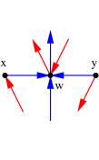
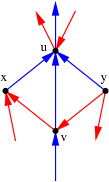
  Figure 25: Decontraction of case b.0 when there is a blue edge leaving $w$ by above.

  Similarly as the previous case the balanced property is preserved (see Figure 26 for an example). So we obtain a balanced transversal structure of $G$.

  

  

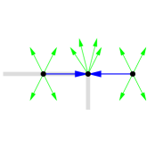
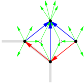
  Figure 26: Decontraction of case b.0 preserving $\gamma$.

• $e_{wx}$ and $e_{wy}$ are not identified and in opposite intervals:

  W.l.o.g., we might assume that we are in case c.0 of Figure 22, i.e. $e_{wx}$ (resp. $e_{wy}$) is entering (resp. leaving) $w$ in color blue. We apply coloring c.1 to $G$. One can easily check that the local property is satisfied around every vertex of $G$ thus we obtain a transversal structure of $G$. Similarly as before the balanced property is preserved and we obtain a balanced transversal structure of $G$.

• $e_{wx}$ and $e_{wy}$ are identified:

  W.l.o.g., we might assume that we are in case d.0 of Figure 22. We apply coloring d.1 to $G$. One can easily check that the local property is satisfied around every vertex of $G$ thus we obtain a transversal structure of $G$. Similarly as before the balanced property is preserved and we obtain a balanced transversal structure of $G$.

For each different possible orientations and colorings of edges $e_{wx}$ and $e_{wy}$ we are able to extend the balanced transversal structure of $G^{\prime}$ to $G$ and thus obtain the result. $\Box$

4.4 Existence theorem

We are now able to prove the existence of balanced transversal structure:

Theorem 2

A toroidal triangulation admits a balanced transversal structure if and only if it is essentially 4-connected.

Proof. ($\Longrightarrow$) Clear by Lemma 4.

($\Longleftarrow$) Let $G$ be an essentially 4-connected toroidal triangulation. By Lemma 12, it can be contracted to a map on one vertex by keeping the map an essentially 4-connected toroidal triangulation. Since during the contraction process, the universal cover is 4-connected, all the vertices have degree at least $4$. The toroidal triangulation on one vertex admits a transversal structure. One such example is given on Figure 12 where one can check that all non-contractible cycles (the three loops) have value $\gamma=0$, and so the transversal structure is balanced. Then, by Lemma 15 applied successively, one can decontract this balanced transversal structure to obtain a balanced transversal structure of $G$. $\Box$

5 Distributive lattice of balanced 4-orientations

5.1 Transformations between balanced 4-orientations

Consider an essentially 4-connected toroidal triangulation $G$ and its angle map $A(G)$. In [GKL16, Theorem 4.7], it is proved that the set of homologous orientations of a given map on an orientable surface carries a structure of distributive lattice. We want to use such a result for the set of balanced $4$-orientations of $A(G)$. For that purpose we prove in this section that balanced $4$-orientations are homologous to each other, i.e. the set of edges that have to be reversed to transform one balanced $4$-orientation into another is a 0-homologous oriented subgraph.

If $D,D^{\prime}$ are two orientations of $A(G)$, let $D\setminus D^{\prime}$ denote the subgraph of $D$ induced by the edges that are not oriented as in $D^{\prime}$. We have the following:

Lemma 16

Let $D$ be a balanced $4$-orientation of $A(G)$. An orientation $D^{\prime}$ of $A(G)$ is a balanced $4$-orientation if and only if $D,D^{\prime}$ are homologous (i.e. $D\setminus D^{\prime}$ is $0$-homologous).

Proof. Let $T=D\setminus D^{\prime}$. Let ${Out}$ (resp. ${Out}^{\prime}$) be the set of edges of $D$ (resp. $D^{\prime}$) which are going from a primal-vertex to a dual-vertex. Note that an edge of $T$ is either in ${Out}$ or in ${Out}^{\prime}$, so $\phi(T)=\phi({Out})-\phi({Out}^{\prime})$. Consider two cycles $B_{1},B_{2}$ of $G$, given with a direction of traversal, that form a basis for the homology. We also denote by $D,D^{\prime}$ the orientation of $\widehat{{A(G)}}$ corresponding to $D,D^{\prime}$. Then we denote $\gamma_{D}$, $\delta_{D}$, $\gamma_{D^{\prime}}$, $\delta_{D^{\prime}}$, the function $\gamma$ and $\delta$ computed in $D$ and $D^{\prime}$ respectively (see terminology of Section 3).

$(\Longrightarrow)$ Suppose $D^{\prime}$ is a balanced $4$-orientation of $A(G)$. Since $D,D^{\prime}$ are both $4$-orientations of $A(G)$, they have the same outdegree for every vertex of $A(G)$. So we have that $T$ is Eulerian. Let $\widehat{\mathcal{F}}^{*}$ be the set of counterclockwise facial walks of $\widehat{{A(G)}}^{*}$, so for any $F\in\widehat{\mathcal{F^{*}}}$, we have $\beta(T,F)=0$. Moreover, for $i\in\{1,2\}$, consider the region $R_{i}$ between $W_{L}(B_{i})$ and $W_{R}(B_{i})$ containing $B_{i}$. Since $T$ is Eulerian, it is going in and out of $R_{i}$ the same number of times. So $\beta(T,W_{L}(B_{i})-W_{R}(B_{i}))=0$ and by linearity of function $\beta$ we obtain $\beta(T,W_{L}(B_{i}))=\beta(T,W_{R}(B_{i}))$. Since $D,D^{\prime}$ are balanced, we have $\gamma_{D}(B_{i})=\gamma_{D^{\prime}}(B_{i})=0$. So by Lemma 11, $\delta_{D}(W_{L}(B_{i}))+\delta_{D}(W_{R}(B_{i}))=\delta_{D^{\prime}}(W_{L}(B_{i}))+\delta_{D^{\prime}}(W_{R}(B_{i}))$. Thus $\beta(T,W_{L}(B_{i})+W_{R}(B_{i}))=\beta(Out-Out^{\prime},W_{L}(B_{i})+W_{R}(B_{i}))=\delta_{D}(W_{L}(B_{i}))+\delta_{D}(W_{R}(B_{i}))-\delta_{D^{\prime}}(W_{L}(B_{i}))-\delta_{D^{\prime}}(W_{R}(B_{i}))=0$. By linearity of function $\beta$ we obtain $\beta(T,W_{L}(B_{i})=-\beta(T,W_{R}(B_{i}))$. By combining this with the above equality, we obtain $\beta(T,W_{L}(B_{i}))=\beta(T,W_{R}(B_{i}))=0$ for $i\in\{1,2\}$. Since $\{W_{L}(B_{1}),W_{L}(B_{2})\}$ form a basis for the homology of $\widehat{{A(G)}}^{*}$, we obtain, by Lemma 7, that $T$ is 0-homologous and so $D,D^{\prime}$ are homologous to each other.

$(\Longleftarrow)$ Suppose that $D,D^{\prime}$ are homologous, i.e. $T$ is $0$-homologous. Then $T$ is in particular Eulerian, so $D^{\prime}$ as the same outdegrees as $D$. So $D^{\prime}$ is a $4$-orientation of $A(G)$. By Lemma 7, for $i\in\{1,2\}$, we have $\beta(T,W_{L}(B_{i}))=\beta(T,W_{R}(B_{i}))=0$. Thus $\delta_{D}(W_{L}(B_{i}))=\beta(Out,W_{L}(B_{i}))+2\beta({Dual},W_{L}(B_{i}))=\beta(Out^{\prime},W_{L}(B_{i}))+2\beta({Dual},W_{L}(B_{i}))=\delta_{D^{\prime}}(W_{L}(B_{i}))$ and $\delta_{D}(W_{R}(B_{i}))=\beta(Out,W_{R}(B_{i}))+2\beta({Dual},W_{R}(B_{i}))=\beta(Out^{\prime},W_{R}(B_{i}))+2\beta({Dual},W_{R}(B_{i}))=\delta_{D^{\prime}}(W_{R}(B_{i}))$. So by Lemma 11, $\gamma_{D}(B_{i})=\delta_{D}(W_{L}(B_{i}))+\delta_{D}(W_{R}(B_{i}))=\delta_{D^{\prime}}(W_{L}(B_{i}))+\delta_{D^{\prime}}(W_{R}(B_{i}))=\gamma_{D^{\prime}}(B_{i})$. Since $D$ is balanced, we have $\gamma_{D}(B_{i})=0$ and so $\gamma_{D^{\prime}}(B_{i})=0$. Then, by Lemma 14, we have $D^{\prime}$ is a balanced $4$-orientation of $A(G)$. $\Box$

5.2 Distributive lattice of homologous orientations

Consider a partial order $\leq$ on a set $S$. Given two elements $x,y$ of $S$, let $m(x,y)$ (resp. $M(x,y)$) be the set of elements $z$ of $S$ such that $z\leq x$ and $z\leq y$ (resp. $z\geq x$ and $z\geq y$). If $m(x,y)$ (resp. $M(x,y)$) is not empty and admits a unique maximal (resp. minimal) element, we say that $x$ and $y$ admit a meet (resp. a join), noted $x\vee y$ (resp. $x\wedge y$). Then $(S,\leq)$ is a lattice if any pair of elements of $S$ admits a meet and a join. Thus in particular a lattice has a unique maximal (resp. minimal) element. A lattice is distributive if the two operators $\vee$ and $\wedge$ are distributive on each other.

Consider an essentially 4-connected toroidal triangulation $G$ and its angle map $A(G)$. By Theorem 2, $G$ admits a balanced transversal structure, thus $A(G)$ admits a balanced $4$-orientation. Let $D_{0}$ be a particular balanced $4$-orientation of $A(G)$. Let $\mathcal{B}(A(G),D_{0})$ be the set of all the orientations of $A(G)$ homologous to $D_{0}$. A general result of [GKL16, Theorem 4.7] concerning the lattice structure of homologous orientations implies that $\mathcal{B}(A(G),D_{0})$ carries a structure of a distributive lattice.

Note that by Lemma 16, the set $\mathcal{B}(A(G),D_{0})$ is exactly the set of all balanced $4$-orientations of $A(G)$. Thus we can simplify the notations and denote $\mathcal{B}(A(G))$ the set $\mathcal{B}(A(G),D_{0})$ as it does not depend on the choice of $D_{0}$.

We give below some terminology and results from [GKL16] adapted to our settings in order to describe the lattice properly. We need to define an order on $\mathcal{B}(A(G))$ for that purpose. Fix an arbitrary face $f_{0}$ of $A(G)$ and let $F_{0}$ be its counterclockwise facial walk. Note that fixing a face $f_{0}$ of $A(G)$ corresponds to fixing an edge $e_{0}$ of $G$. Let $\mathcal{F}$ be the set of counterclockwise facial walks of $A(G)$ and $\mathcal{F}^{\prime}=\mathcal{F}\setminus\{F_{0}\}$. Note that $\phi(F_{0})=-\sum_{F\in\mathcal{F}^{\prime}}\phi(F)$. Since the characteristic flows of $\mathcal{F}^{\prime}$ are linearly independent, any oriented subgraph of $A(G)$ has at most one representation as a combination of characteristic flows of $\mathcal{F}^{\prime}$. Moreover the $0$-homologous oriented subgraphs of $A(G)$ are precisely the oriented subgraph that have such a representation. We say that a $0$-homologous oriented subgraph $T$ of $A(G)$ is counterclockwise (resp. clockwise) w.r.t. $f_{0}$ if its characteristic flow can be written as a combination with positive (resp. negative) coefficients of characteristic flows of $\mathcal{F}^{\prime}$, i.e. $\phi(T)=\sum_{F\in\mathcal{F}^{\prime}}\lambda_{F}\phi(F)$, with $\lambda\in\mathbb{N}^{|\mathcal{F}^{\prime}|}$ (resp. $-\lambda\in\mathbb{N}^{|\mathcal{F}^{\prime}|}$). Given two orientations $D,D^{\prime}$, of $A(G)$ we set $D\leq_{f_{0}}D^{\prime}$ if and only if $D\setminus D^{\prime}$ is counterclockwise. Then we have the following theorem:

Theorem 3 ([GKL16])

$(\mathcal{B}(A(G)),\leq_{f_{0}})$ is a distributive lattice.

To define the elementary flips that generates the lattice. We start by reducing the graph $A(G)$. We call an edge of $A(G)$ rigid with respect to $\mathcal{B}(A(G))$ if it has the same orientation in all elements of $\mathcal{B}(A(G))$. Rigid edges do not play a role for the structure of $\mathcal{B}(A(G))$. We delete them from $A(G)$ and call the obtained embedded graph the reduced angle graph, noted $\widetilde{A(G)}$. Note that, this graph is embedded but it is not necessarily a map, as some faces may not be homeomorphic to open disks. Note that if all the edges are rigid, then $|\mathcal{B}(A(G))|=1$ and $\widetilde{A(G)}$ has no edges. We have the following lemma concerning rigid edges:

Lemma 17 ([GKL16, Lemma 4.8])

Given an edge $e$ of $A(G)$, the following are equivalent:

1. $e$ is non-rigid

2. $e$ is contained in a $0$-homologous oriented subgraph of $D_{0}$

3. $e$ is contained in a $0$-homologous oriented subgraph of any element of $\mathcal{B}(A(G))$

By Lemma 17, one can build $\widetilde{A(G)}$ by keeping only the edges that are contained in a $0$-homologous oriented subgraph of $D_{0}$. Note that this implies that all the edges of $\widetilde{A(G)}$ are incident to two distinct faces of $\widetilde{A(G)}$. Denote by $\widetilde{\mathcal{F}}$ the set of oriented subgraphs of $\widetilde{A(G)}$ corresponding to the boundaries of faces of $\widetilde{A(G)}$ considered counterclockwise. Note that any $\widetilde{F}\in\widetilde{\mathcal{F}}$ is $0$-homologous and so its characteristic flow has a unique way to be written as a combination of characteristic flows of $\mathcal{F}^{\prime}$. Moreover this combination can be written $\phi(\widetilde{F})=\sum_{F\in X_{\widetilde{F}}}\phi(F)$, for $X_{\widetilde{F}}\subseteq\mathcal{F}^{\prime}$. Let $\widetilde{f}_{0}$ be the face of $\widetilde{A(G)}$ containing $f_{0}$ and $\widetilde{F}_{0}$ be the element of $\widetilde{\mathcal{F}}$ corresponding to the boundary of $\widetilde{f}_{0}$. Let $\widetilde{\mathcal{F}}^{\prime}=\widetilde{\mathcal{F}}\setminus\{\widetilde{F}_{0}\}$. The elements of $\widetilde{\mathcal{F}}^{\prime}$ are precisely the elementary flips which suffice to generate the entire distributive lattice $(\mathcal{B}(A(G)),\leq_{f_{0}})$, i.e. the Hasse diagram $\mathcal{H}$ of the lattice has vertex set $\mathcal{B}(A(G))$ and there is an oriented edge from $D_{1}$ to $D_{2}$ in $\mathcal{H}$ (with $D_{1}\leq_{f_{0}}D_{2}$) if and only if $D_{1}\setminus D_{2}\in\widetilde{\mathcal{F}}^{\prime}$.

Moreover, we have:

Lemma 18 ([GKL16, Proposition 4.13])

For every element $\widetilde{F}\in\widetilde{\mathcal{F}}$, there exists $D$ in $\mathcal{B}(A(G))$ such that $\widetilde{F}$ is an oriented subgraph of $D$.

By Lemma 18, for every element $\widetilde{F}\in\widetilde{\mathcal{F}}^{\prime}$ there exists $D$ in $\mathcal{B}(A(G))$ such that $\widetilde{F}$ is an oriented subgraph of $D$. Thus there exists $D^{\prime}$ such that $\widetilde{F}=D\setminus D^{\prime}$ and $D,D^{\prime}$ are linked in $\mathcal{H}$. Thus $\widetilde{\mathcal{F}}^{\prime}$ is a minimal set that generates the lattice.

Let $D_{\max}$ (resp. $D_{\min}$) be the maximal (resp. minimal) element of the lattice $(\mathcal{B}(A(G)),\leq_{f_{0}})$. Then we have the following lemmas:

Lemma 19 ([GKL16, Proposition 4.14])

$\widetilde{F}_{0}$ (resp. $-\widetilde{F}_{0}$) is an oriented subgraph of $D_{\max}$ (resp. $D_{\min}$).

Lemma 20 ([GKL16, Proposition 4.15])

$D_{\max}$ (resp. $D_{\min}$) contains no counterclockwise (resp. clockwise) non-empty $0$-homologous oriented subgraph w.r.t. $f_{0}$.

Note that in the definition of counterclockwise (resp. clockwise) non-empty $0$-homologous oriented subgraph, used in Lemma 20, the sum is taken over elements of $\mathcal{F}^{\prime}$ and thus does not use $F_{0}$. In particular, $D_{\max}$ (resp. $D_{\min}$) may contain regions whose boundary is oriented counterclockwise (resp. clockwise) according to the interior of the region but then such a region contains $f_{0}$ in its interior.

Note that, assuming that an element of $\mathcal{B}(A(G))$ is given, there is a generic method to compute in linear time the minimal balanced element $D_{\min}$ of $(\mathcal{B}(A(G)),\leq_{f_{0}})$ (see [DGL17, last paragraph of Section 8]. This minimal element plays the role of a canonical orientation and is particularly interesting for bijection purpose as shown in Section 6.

5.3 Faces of the reduced angle graph

Previous section is about the general situation of the lattice structure of homologous orientations and is more or less a copy/paste from [GKL16] of the terminology and results that we need here. Now we study in more detail this lattice w.r.t. the balanced property as done in [DGL17, Section 10] for Schnyder woods and $3$-orientations (see also [Lév17, Section 8.4]).

Consider an essentially 4-connected toroidal triangulation $G$ and its angle map $A(G)$. We consider the terminology of the previous section and assume that there exists a balanced $4$-orientation $D_{0}$ of $A(G)$.

We say that a walk $W$ of $A(G)$ is a $4$-disk if it is a face of $A(G)$ (see the left of Figure 27). We say that a walk $W$ of $A(G)$ is a $8$-disk if it has size $8$, encloses a region $R$ homeomorphic to an open disk and the dual-vertices of $W$ have their edge not on $W$ that is inside $R$ (see the right of Figure 27). Finally, we say that a walk $W$ of $A(G)$ is a $\{4,8\}$-disk if it is either a $4$-disk or a $8$-disk.

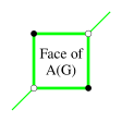
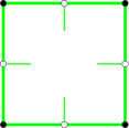
$4$-disk	$8$-disk

Figure 27: The $\{4,8\}$-disks of $A(G)$.

Suppose that $A(G)$ is given with a 4-orientation. For an edge $e_{0}$ of $A(G)$ we define the left walk (resp. right walk) from $e_{0}$ as the sequence of edges $W=(e_{i})_{i\geq 0}$ of $A(G)$ obtained by the following: if $e_{i}$ is entering a primal-vertex $v$, then $e_{i+1}$ is the first outgoing edge while going clockwise (resp. counterclockwise ) around $v$ from $e_{i}$, and if $e_{i}$ is entering a dual-vertex $v^{*}$, then $e_{i+1}$ is the only outgoing edge of $v^{*}$. A closed left/right walk is a left/right walk that is repeating periodically on itself, i.e. a finite sequence of edges $W=(e_{i})_{0\leq i\leq 2k-1}$, with $k>0$, such that its repetition is a left/right walk. We have the following lemma concerning closed left/right walks in balanced $4$-orientations:

Lemma 21

In a balanced $4$-orientation of $A(G)$, a closed left (resp. right) walk $W$ of $A(G)$ encloses a region homeomorphic to an open disk on its left (resp. right) side. Moreover, the border of this region is a $\{4,8\}$-disk.

Proof. Consider a closed left walk $W=(e_{i})_{0\leq i\leq 2k-1}$ of $A(G)$, with $k>0$. W.l.o.g., we may assume that all the $e_{i}$ are distinct, i.e. there is no strict subwalk of $W$ that is also a closed left walk. Note that $W$ cannot cross itself otherwise it is not a left walk. However $W$ may have repeated vertices but in that case it intersects itself tangentially on the right side.

Suppose by contradiction that there is an oriented subwalk $W^{\prime}$ of $W$, that forms a cycle $C$ enclosing a region $R$ on its right side that is homeomorphic to an open disk. Let $v$ be the starting and ending vertex of $W^{\prime}$. Note that we do not consider that $W^{\prime}$ is a strict subwalk of $W$, so we might have $W^{\prime}=W$. Consider the graph $H$ obtained from $A(G)$ by keeping all the vertices and edges that lie in the region $R$, including $W^{\prime}$. Since $W$ can intersect itself only tangentially on the right side, we have that $H$ is a bipartite planar map whose outer face boundary is $W^{\prime}$. The inner faces of $H$ are quadrangles. Let $2k^{\prime}$ be the length of $W^{\prime}$. Let $n^{\prime},m^{\prime},f^{\prime}$ be the number of vertices, edges and faces of $H$. By Euler’s formula, $n^{\prime}-m^{\prime}+f^{\prime}=2$. All the inner faces have size $4$ and the outer face has size $2k^{\prime}$, so $2m^{\prime}=4(f^{\prime}-1)+2k^{\prime}$. Combining the two equalities gives $m^{\prime}=2n^{\prime}-k^{\prime}-2$. Let $n_{p}^{\prime}$ (resp. $n^{\prime}_{d}$) be the number of inner primal-vertices (resp. inner dual-vertices) of $H$. So $n^{\prime}=2k^{\prime}+n_{p}^{\prime}+n_{d}^{\prime}$ and thus $m^{\prime}=2n_{p}^{\prime}+2n_{d}^{\prime}+3k^{\prime}-2$. Since $W^{\prime}$ is a subwalk of a left walk, all primal-vertices of $H$, except $v$ (if it is a primal-vertex), have their incident outer edges in $H$. Since $W^{\prime}$ is following oriented edges, if $v$ is a primal vertex, it has at least one outgoing edge in $H$. Since we are considering a $4$-orientation of $A(G)$, we have $m^{\prime}\geq 4(k^{\prime}-1)+1+4n_{p}^{\prime}+n_{d}^{\prime}$. By counting the edges of $H$ incident to dual-vertices, we have $m^{\prime}\geq 2k^{\prime}+3n_{d}^{\prime}$. Combining the three (in)equalities of $m^{\prime}$, gives $2(2n_{p}^{\prime}+2n_{d}^{\prime}+3k^{\prime}-2)\geq(4(k^{\prime}-1)+1+4n_{p}^{\prime}+n_{d}^{\prime})+(2k^{\prime}+3n_{d}^{\prime})$, a contradiction. So there is no oriented subwalk of $W$, that forms a cycle enclosing an open disk on its right side.

We now claim the following:

Claim 2

The left side of $W$ encloses a region homeomorphic to an open disk

Proof.  We consider two cases depending on the fact that $W$ is a cycle (i.e. with no repetition of vertices) or not.

• $W$ is a cycle

  Suppose by contradiction that $W$ is a non-contractible cycle. For each dual-vertex of $W$, there is an edge of $G$ between its neighbors in $W$. This edge might be either on the left or right side of $W$. Consider the cycle $C$ of $G$ made of all these edges. Since we are considering a balanced $4$-orientation of $A(G)$, we have $\gamma(C)=0$ and thus there is exactly $2k$ outgoing edges of $A(G)$ that are incident to the left side of $C$. There is no incident outgoing edge of $A(G)$ on the left side of $W$. So the outgoing edges that are on the left side of $C$ are exactly the $2k$ edges of $W$. So $C$ is completely on the right side of $W$ and all the edges of $W$ are outgoing for primal-vertices. Thus all dual-vertices have an outgoing edge on the left side of $W$, a contradiction. Thus $W$ is a contractible cycle.

  As explained above, the contractible cycle $W$ does not enclose a region homeomorphic to an open disk on its right side. So $W$ encloses a region homeomorphic to an open disk on its left side, as claimed.

• $W$ is not a cycle

  Since $W$ cannot cross itself nor intersect itself tangentially on the left side, it has to intersect tangentially on the right side. Such an intersection on a vertex $v$ is depicted on Figure 28.(a). The edges of $W$ incident to $v$ are noted as on the figure, $a,b,c,d$, where $W$ is going periodically through $a,b,c,d$ in this order. The (green) subwalk of $W$ from $a$ to $b$ does not enclose a region homeomorphic to an open disk on its right side. So we are not in the case depicted on Figure 28.(b). Moreover if this (green) subwalk encloses a region homeomorphic to an open disk on its left side, then this region contains the (red) subwalk of $W$ from $c$ to $d$, see Figure 28.(c). Since $W$ cannot cross itself, this (red) subwalk necessarily encloses a region homeomorphic to an open disk on its right side, a contradiction. So the (green) subwalk of $W$ starting from $a$ has to form a non-contractible curve before reaching $b$. Similarly for the (red) subwalk starting from $c$ and reaching $d$. Since $W$ is a left-walk and cannot cross itself, we are, w.l.o.g., in the situation of Figure 28.(d) (with possibly more tangent intersections on the right side). In any case, the left side of $W$ encloses a region homeomorphic to an open disk.

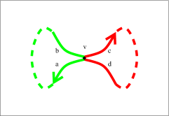
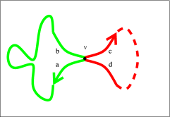
  (a)	(b)
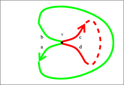
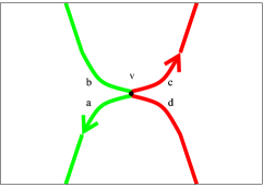
  (c)	(d)

  Figure 28: Case analysis for the proof of Claim 2.

$\Diamond$

By Claim 2, the left side of $W$ encloses a region $R$ homeomorphic to an open disk. Consider the graph $H$ obtained from $A(G)$ by keeping only the vertices and edges that lie in $R$, including $W$. The vertices of $W$ appearing several times on the border of $R$ are duplicated, so $H$ is a bipartite planar map. The inner faces of $H$ are quadrangles. As above, let $n^{\prime},m^{\prime},f^{\prime}$ be the number of vertices, edges and faces of $H$ and $n_{p}^{\prime}$ (resp. $n^{\prime}_{d}$) its number of inner primal-vertices (resp. inner dual-vertices). So as above, one obtain the first equality $m^{\prime}=2n_{p}^{\prime}+2n_{d}^{\prime}+3k-2$. There is no incident outgoing edge of $A(G)$ on the left side of $W$. So all inner edges of $H$ are outgoing for inner vertices of $H$. Since we are considering a $4$-orientation of $A(G)$, we have $m^{\prime}=2k+4n_{p}^{\prime}+n_{d}^{\prime}$. Outer dual-vertices of $H$ might be of degree $2$ or $3$ in $H$. Let $x$ be the number of outer dual-vertices of $H$ of degree $3$ in $H$, so by counting the edges of $H$ incident to dual-vertices we have $m^{\prime}=2k+x+3n_{d}^{\prime}$. Combining the three equalities of $m^{\prime}$, gives $2(2n_{p}^{\prime}+2n_{d}^{\prime}+3k-2)=(2k+4n_{p}^{\prime}+n_{d}^{\prime})+(2k+x+3n_{d}^{\prime})$, so $x=2k-4$. Since $k\geq x\geq 0$, the only possible values are $(k,x)\in\{(2,0),(3,2),(4,4)\}$.

If $(k,x)=(2,0)$, then $W$ has size four, its two dual-vertices are of degree $2$ in $H$ so they have their edge not on $W$ that is outside $R$. If $W$ is not a face of $A(G)$, then there are two distinct edges between the primal-vertices of $W$ inside $R$, forming a pair of homotopic multiple edges, a contradiction. So $W$ is a face of $A(G)$ and thus a $4$-disk. If $(k,x)=(3,2)$, then $W$ has size six, with two dual-vertices of degree $3$ in $H$ and $G^{\infty}$ has a separating triangle, a contradiction to Lemma 5. If $(k,x)=(4,4)$, then $W$ has size eight, with its four dual-vertices of degree $3$ in $H$. So $W$ is a $8$-disk.

The proof is similar for closed right walks. $\Box$

The boundary of a face of $\widetilde{A(G)}$ may be composed of several closed walks. Let us call quasi-contractible the faces of $\widetilde{A(G)}$ that are homeomorphic to an open disk or to an open disk with punctures. Note that such a face may have several boundaries (if there is some punctures), but exactly one of these boundaries encloses the face. Let us call outer facial walk this special boundary. Then we have the following:

Lemma 22

All the faces of $\widetilde{A(G)}$ are quasi-contractible and their outer facial walk is a $\{4,8\}$-disk.

Proof. Consider a face $\widetilde{f}$ of $\widetilde{A(G)}$. Let $\widetilde{F}$ be the element of $\widetilde{\mathcal{F}}$ corresponding to the boundary of $\widetilde{f}$. By Lemma 18, there exists $D\in\mathcal{B}(A(G))$ such that $\widetilde{F}$ is an oriented subgraph of $D$.

All the faces of $A(G)$ form a $4$-disk. Thus either $\widetilde{f}$ is a face of $A(G)$ and we are done or $\widetilde{f}$ contains in its interior at least one edge of $A(G)$. Start from such edge $e_{0}$ and consider the left-walk $W=(e_{i})_{i\geq 0}$ of $D$ from $e_{0}$. Suppose that for $i\geq 0$, edge $e_{i}$ is entering a vertex $v$ that is on the border of $\widetilde{f}$. Recall that by definition $\widetilde{F}$ is oriented counterclockwise according to its interior, so either $e_{i+1}$ is in the interior of $\widetilde{f}$ or $e_{i+1}$ is on the border of $\widetilde{f}$. Thus $W$ cannot leave $\widetilde{f}$ and its border.

Since $A(G)$ has a finite number of edges, some edges are used several times in $W$. Consider a minimal subsequence $W^{\prime}=e_{k},\ldots,e_{\ell}$ such that no edge appears twice and $e_{k}=e_{\ell+1}$. Thus $W$ ends periodically on $W^{\prime}$ that is a closed left walk. By Lemma 21, $W^{\prime}$ encloses a region $R$ homeomorphic to an open disk on its left side. Moreover, the border of this region is a $\{4,8\}$-disk. Thus $W^{\prime}$ is a $0$-homologous oriented subgraph of $D$. So all its edges are non-rigid by Lemma 17. So all the edges of $W^{\prime}$ are part of the border of $\widetilde{f}$. Since $\widetilde{F}$ is oriented counterclockwise according to its interior, the region $R$ contains $\widetilde{f}$. So $\widetilde{f}$ is quasi-contractible and $W^{\prime}$ is its outer facial walk and a $\{4,8\}$-disk. $\Box$

A simple counting argument gives the following lemma (see Figure 29):

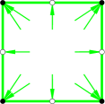
Figure 29: Orientation of inner edges incident to a $8$-disk.

Lemma 23

In a $4$-orientation of $A(G)$, the edges that are in the interior of a $8$-disk and incident to it are entering it.

Proof. Consider a $8$-disk $W$ of $A(G)$. Consider the graph $H$ obtained from $A(G)$ by keeping only the vertices and edges that lie in $W$ and its interior. The vertices of $W$ appearing several times on $W$ are duplicated, so $H$ is a bipartite planar map. Let $x$ be the number of inner-edges of $H$ that are incident to its outer-face and directed toward the interior. We want to prove that $x=0$.

Let $n^{\prime},m^{\prime},f^{\prime}$ be the number of vertices, edges and faces of $H$. By Euler’s formula, $n^{\prime}-m^{\prime}+f^{\prime}=2$. All the inner faces have size $4$ and the outer face has size $8$, so $2m^{\prime}=4(f^{\prime}-1)+8$. Combining the two equalities gives $m^{\prime}=2n^{\prime}-6$. Let $n_{p}^{\prime}$ (resp. $n^{\prime}_{d}$) be the number of inner primal-vertices (resp. inner dual-vertices) of $H$. So $n^{\prime}=n_{p}^{\prime}+n_{d}^{\prime}+8$ and thus $m^{\prime}=2n_{p}^{\prime}+2n_{d}^{\prime}+10$. Since we are considering a $4$-orientation of $A(G)$, we have $m^{\prime}=4n_{p}^{\prime}+n_{d}^{\prime}+x+8$. By counting the edges of $H$ incident to dual-vertices we have $m^{\prime}=3n_{d}^{\prime}+12$. Combining the three equalities of $m^{\prime}$, gives $2(2n_{p}^{\prime}+2n_{d}^{\prime}+10)=(4n_{p}^{\prime}+n_{d}^{\prime}+x+8)+(3n_{d}^{\prime}+12)$, so $x=0$.

$\Box$

We say that a $\{4,8\}$-disk of $A(G)$ is maximal (by inclusion) if its interior is not strictly contained in the interior of another $\{4,8\}$-disk of $A(G)$.

Lemma 24

There is a unique maximal $\{4,8\}$-disk of $A(G)$ containing $f_{0}$ and it is oriented counterclockwise (resp. clockwise) in $D_{\max}$ (resp. $D_{\min}$).

Proof. By Lemma 22, $\widetilde{f}_{0}$ is quasi-contractible and its outer facial walk is a $\{4,8\}$-disk. So there is a $\{4,8\}$-disk containing $f_{0}$. Let $W$ be a maximal $\{4,8\}$-disk containing $f_{0}$. By Lemma 23, if $W$ is a $8$-disk, then, for any $4$-orientation of $A(G)$, the edges of $A(G)$ that are in the interior of $W$ and incident to it are entering it. If $W$ is a $4$-disk, then there is no edge of $A(G)$ in the interior of $W$. So all the edges in the interior of $W$ and incident to it are rigid edges, i.e. these edges are not in $\widetilde{A(G)}$. So there is a face $\widetilde{f}$ of $\widetilde{A(G)}$ containing all the faces $F_{W}$ of $A(G)$ that are in the interior of $W$ and incident to it. Note that there might be some punctures in $\widetilde{f}$, so $\widetilde{f}$ does not necessarily contain all the faces of $A(G)$ that are in the interior of $W$. By Lemma 22, $\widetilde{f}$ is quasi-contractible and its outer facial walk is a $\{4,8\}$-disk. By maximality of $W$, the $\{4,8\}$-disk $W$ is the only $\{4,8\}$-disk of $A(G)$ containing the faces $F_{W}$. So the outer facial walk of $\widetilde{f}$ is $W$ and all the edges of $W$ are non-rigid, i.e. these edges are in $\widetilde{A(G)}$.

Suppose by contradiction that there exists another maximal $\{4,8\}$-disk $W^{\prime}$ containing $f_{0}$ that is distinct from $W$. As for $W$, all the edges of $W^{\prime}$ are in $\widetilde{A(G)}$. The interiors of $W$ and $W^{\prime}$ have to be distinct, not included one into each other, but intersecting. Then at least one edge of $W^{\prime}$ has to be in the interior of $W$ and incident to it, a contradiction to the fact that these edges are not in $\widetilde{A(G)}$. So $W$ is the unique maximal $\{4,8\}$-disk containing $f_{0}$.

We now prove the second part of the lemma for $D_{\max}$ (the proof is similar for $D_{\min}$). Let $\widetilde{F}$ be the element of $\widetilde{\mathcal{F}}$ corresponding to the boundary of $\widetilde{f}$. We consider two cases depending on the fact that $\widetilde{f}$ is equal to $\widetilde{f}_{0}$ or not, i.e. $\widetilde{f}=\widetilde{f}_{0}$ or $\widetilde{f}$ has some punctures, one of which contains $\widetilde{f}_{0}$.

• $\widetilde{f}=\widetilde{f}_{0}$: By Lemma 19, we have $\widetilde{F}=\widetilde{F}_{0}$ is an oriented subgraph of $D_{\max}$ and thus $W$ is oriented counterclockwise w.r.t. its interior.

• $\widetilde{f}\neq\widetilde{f}_{0}$: By Lemma 18, there exists an element of $\mathcal{B}(A(G))$ for which $\widetilde{F}$ is an oriented subgraph. Let $D$ be such an element, chosen such that $\widetilde{F}$ is not an oriented subgraph of any orientation, distinct from $D$, that is on oriented paths from $D$ to $D_{\max}$ in the Hasse diagram of $(\mathcal{B}(A(G)),\leq_{f_{0}})$. The $\{4,8\}$-disk $W$ is oriented counterclockwise in $D$. Recall that $\widetilde{f}$ has at least one puncture containing $\widetilde{f}_{0}$.

  Let $D^{\prime}$ be the orientation obtained from $D$ by reversing all the edges of $\widetilde{f}$ that are not on its outer facial walk, i.e. obtained by reversing the border of all the punctures. So the $\{4,8\}$-disk $W$ is still oriented counterclockwise in $D^{\prime}$. We claim that $D,D^{\prime}$ are such that $D\leq_{f_{0}}D^{\prime}$. Indeed, let $T=D\setminus D^{\prime}$ and $X$ denote the set of all the elements of $\mathcal{F}^{\prime}$ that corresponds to faces of $A(G)$ that are not in the punctures of $\widetilde{f}$. Then we have $\phi(T)=\sum_{{F}\in X}\phi({F})$ and $X$ is a subset of ${\mathcal{F}}^{\prime}$. So $D\leq_{f_{0}}D^{\prime}$. Consider $D^{\prime}=D_{0},\ldots,D_{k}=D_{\max}$, with $k\geq 0$, the elements of $\mathcal{B}(A(G))$ on an oriented path from $D^{\prime}$ to $D_{\max}$ in the Hasse diagram of $(\mathcal{B}(A(G)),\leq_{f_{0}})$.

  Suppose by contradiction that the $\{4,8\}$-disk $W$ is not oriented counterclockwise in $D_{\max}$. Let $1\leq i\leq k$ be the minimal integer such that the $\{4,8\}$-disk $W$ is not oriented counterclockwise in $D_{i}$. Thus the $\{4,8\}$-disk $W$ is oriented counterclockwise in $D_{i-1}$ but not in $D_{i}$. Since $D_{i-1}$ and $D_{i}$ are linked in the Hasse diagram, we have $D_{i-1}\setminus D_{i}\in\widetilde{\mathcal{F}}^{\prime}$. Let $\widetilde{F}^{\prime}\in\widetilde{\mathcal{F}}^{\prime}$ be such that $\widetilde{F}^{\prime}=D_{i-1}\setminus D_{i}$. By assumption on $D$ we have $\widetilde{F}^{\prime}$ is distinct from $\widetilde{F}$. Moreover, since $W$ is oriented counterclockwise in $D_{i-1}$, we have that $\widetilde{F}^{\prime}$ is distinct from all the elements of $\widetilde{\mathcal{F}}^{\prime}$ corresponding to faces that are incident to $W$ and not in its interior. So $\widetilde{F}^{\prime}$ is disjoint from $W$ and $W$ has the same orientation in $D_{i-1}$ and $D_{i}$, a contradiction. So $W$ is oriented counterclockwise in $D_{\max}$.

$\Box$

5.4 Example of a balanced lattice

Consider the essentially $4$-connected toroidal triangulation $G$ of Figure 1 and its angle map $A(G)$. One example of a balanced $4$-orientation of $A(G)$ is given on the right of Figure 2, we call it $D_{0}$ in this section. By Lemma 17, an edge of $A(G)$ is non-rigid if and only if if is contained in a $0$-homologous oriented subgraph of $D_{0}$. So with this rule, one can build the reduced angle graph $\widetilde{A(G)}$ depicted on Figure 30. One can check that Lemma 22 is satisfied since the faces are made of one 8-disk and some 4-disks. We choose arbitrarily a special face $f_{0}$ of $\widetilde{A(G)}$ as depicted on the figure.

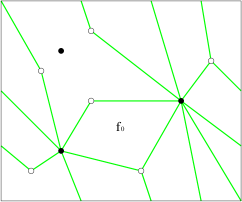
Figure 30: The reduced angle graph of the triangulation of Figure 1.

The set of all orientations of $A(G)$ that are homologous to $D_{0}$ is exactly the set $\mathcal{B}(A(G))$ of all balanced $4$-orientations of $A(G)$ by Lemma 16. Moreover, we have that $(\mathcal{B}(A(G)),\leq_{f_{0}})$ is a distributive lattice by Theorem 3. The Hasse diagram of this lattice is represented on the left of Figure 31. Each node of the diagram is a balanced $4$-orientation of $A(G)$ and black edges are the edges of the diagram.

The orientation on the left of Figure 2 is not in the diagram since it is not balanced. The orientation $D_{0}$, on the right of Figure 2, is the second one starting from the top. The other orientations of the diagram are obtained from $D_{0}$ by flipping oriented faces of the reduced angle graph $\widetilde{A(G)}$, except $f_{0}$.

When a face of the reduced angle graph is oriented this is represented by a circle. The circle is black when it corresponds to the face containing $f_{0}$. The circle is magenta if the boundary of the corresponding face of $\widetilde{A(G)}$ is oriented counterclockwise and cyan otherwise. For the face of $\widetilde{A(G)}$ that is a 8-disk, we represent the circle around the unique vertex that is in the interior of this 8-disk.

An edge in the Hasse diagram from $D$ to $D^{\prime}$ (with $D\leq D^{\prime}$) corresponds to a face of $\widetilde{A(G)}$ oriented counterclockwise in $D$ whose edges are reversed to form a face oriented clockwise in $D^{\prime}$, i.e. a magenta circle replaced by a cyan circle. The outdegree of a node is its number of magenta circle and its indegree is its number of cyan circle. By Lemma 18, all the faces of $\widetilde{A(G)}$ have a circle at least once. The special face is not allowed to be flipped and, by Lemma 19, it is oriented counterclockwise in the maximal element of the lattice and clockwise in the minimal element. By Lemma 20, the maximal (resp. minimal) element contains no other faces of $\widetilde{A(G)}$ oriented counterclockwise (resp. clockwise), indeed it contains only cyan (resp. magenta) circles and one black. One can play with the black circle and see which are the orientations of the lattice that are in correspondence by flipping the face $f_{0}$.

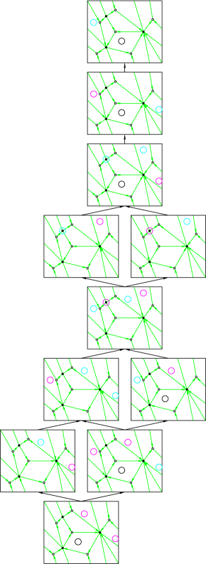
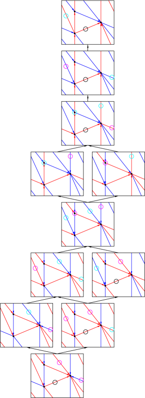
Figure 31: The Hasse diagram of the distributive lattice of the balanced 4-orientations of the angle map of an essentially $4$-connected toroidal triangulation.

All the $4$-orientations of the diagram are balanced so they correspond to transversal structures by Corollary 1. These transversal structures are represented on the right of Figure 31. The lattice may have been defined directly on the transversal structures using the same transformations as in the planar case (see [Fus09, Figure 6 and Theorem 2]). But we prefer to present this by considering $\alpha$-orientations here since it is a more general framework that also enables to use directly results from [GKL16] without re-proving the lattice structure.

6 Bijection with unicellular mobiles

6.1 From essentially 4-connected toroidal triangulations to mobiles

Consider an essentially 4-connected toroidal triangulation $G$ and its angle map $A(G)$. In order to use the lattice structure on the (non-empty) set $\mathcal{B}(A(G))$ we need to choose a particular face of $A(G)$, i.e. a particular edge of $G$. This choice has to be done appropriately so that the minimal element of the lattice have some interesting properties for the bijection. For that purpose, we have to consider quadrangles of $G$. We choose a half-edge $h_{0}$ of $G$ that is in the interior and incident to a maximal quadrangle of $G$. We call $h_{0}$ the root half-edge of $G$. The vertex $v_{0}$ of $G$ incident to $h_{0}$ is called the root vertex. The face $f_{0}$ of $A(G)$ containing $h_{0}$ is called the root face. Consider the order $\leq_{f_{0}}$ define on $\mathcal{B}(A(G))$ in Section 5.2. By Theorem 3, $(\mathcal{B}(A(G)),\leq_{f_{0}})$ forms a distributive lattice. Thus we can consider the minimal balanced $4$-orientation $D_{\min}$ of $\mathcal{B}(A(G))$ w.r.t. $f_{0}$. Since there is no ambiguity, we may also say that $D_{\min}$ is minimal w.r.t. $h_{0}$.

By Corollary 1, $D_{\min}$ corresponds to a transversal structure of $G$ and admits a TTS-labeling (see Section 3.1). By convention, the transversal structure of $G$ associated to $D_{\min}$ that we consider is the one where $h_{0}$ is an outgoing half-edge of color blue, i.e. in the TTS-labeling the half-edge is labeled $0$.

Let us associate to any $4$-orientation $D$ of $A(G)$ a particular graph $M$ embedded on the torus, called mobile associated to $D$. The vertex set of $M$ is the same as $G$. Its edge set is composed of some edges of $G$ plus some half-edges that are incident to only one vertex. We sometimes call the edges of $M$ full-edges to avoid confusion with half-edges of $M$. Moreover we see the full-edges of $M$ as two half-edges of $M$ that meet at the middle of the edge. Then the set of half-edges of $M$ is defined by the following rule: a half-edge $h$ of $G$, incident to a vertex $v$ of $G$, is an half-edge of $M$ if and only if the edge of $D$ just after $h$ in clockwise order around $v$ is outgoing (see Figure 32). If $G$ is rooted on a particular half-edge $h_{0}$, then the extended mobile $M^{+}$ is obtained from $M$ by adding the root half-edge $h_{0}$ if not already in $M$. If the two half-edges of the same edge of $G$ are in $M$ (resp. $M^{+}$), then they meet in order to form a full-edge of $M$ (resp. $M^{+}$). The half-edges of $M$ (resp. $M^{+}$) that are not part of a full-edge of $M$ (resp. $M^{+}$) are called stems and they are presented by an arrow on the figures.

Figure 32: Rule for half-edges of the mobile.

A balanced transversal structure of $K_{7}$ is given on Figure 33 with the corresponding balanced $4$-orientation of its angle map that is minimal w.r.t. the barred half-edge. The extended mobile associated to this orientation is represented twice, once with the angle map and once alone as a hexagon whose opposite sides are identified to form a toroidal map. The vertices are labeled from $1$ to $7$, and the root half-edge is represented in magenta on the figures.

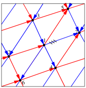
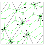
Figure 33: Balanced transversal structure of $K_{7}$, given with the corresponding balanced $4$-orientation of its angle map, that is minimal w.r.t. the barred half-edge, and the corresponding extended mobile, represented as an hexagon whose opposite sides are identified.

Note that the mobile can be computed directly from the transversal structure by considering the following set of half-edges for $M$: an half-edge $h$ of $G$, incident to a vertex $v$ of $G$, is a half-edge of $M$ if and only if it is the last edge of an interval (outgoing blue, outgoing red, incoming blue, incoming red) of $v$ in clockwise order around $v$. This point of view corresponds more to the planar study of transversal structure from [Fus09]. But the rule of Figure 32 corresponds to a more general framework to construct so-called “mobile” that can be applied to any orientation (see [BF12a, BF12b, BC11]) and not only to transversal structure.

Part of the TTS-labeling of $D_{min}$ can be represented on the mobile $M$ by keeping only the labels that are on half-edges of $M$. By the mobile rule, one can note that a mobile-labeling satisfies the following properties: the four labels that appear around each vertex are exactly $0,1,2,3$ in counterclockwise order and the two labels that appear on each edge differ exactly by $(2\bmod 4)$ (see Figure 34 where the TTS-labeling is represented on the transversal structure and on the corresponding mobile).

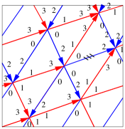
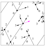
Figure 34: TTS-labeling represented on the mobile.

We say that an edge $e$ of $G$ is covered by $M$ (resp. $M^{+}$) if there is at least one half-edge of $e$ in $M$ (resp. $M^{+}$). We say that a vertex $v$ of $G$ is covered by $M$ (resp. $M^{+}$) if there is at least one half-edge incident to $v$ in $M$ (resp. $M^{+}$).

The main result of this section is the following theorem:

Theorem 4

Consider an essentially 4-connected toroidal triangulation $G$, and a root half-edge $h_{0}$ of $G$ that is in the interior and incident to a maximal quadrangle of $G$. Then the extended mobile $M^{+}$ associated to the minimal balanced $4$-orientation of $A(G)$ w.r.t. $h_{0}$ is a toroidal unicellular map covering all the vertices and edges of $G$. Moreover, either $h_{0}$ is a stem of $M^{+}$ or its removal creates two connected components, one of which is a tree.

Proof. Consider the minimal balanced $4$-orientation $D_{\min}$ of $A(G)$ w.r.t. $h_{0}$, the associated mobile $M$ and the extended mobile $M^{+}$. We consider the superposition of $D_{\min}$ and $M^{+}$ (see the middle of Figure 33).

Let us first prove that $M$ has a unique face. Consider a particular face $F$ of $M$. Note that this face is not necessarily homeomorphic to an open disk (it can be homeomorphic to a torus, a cylinder, a disk, with punctures) so the border of $F$ can be made of several closed walk of $M$. By definition of the mobile $M$, each occurrence of a vertex $v$ on the border of $F$ has an incident edge $e$ of $D_{\min}$ that is outgoing in the interior of $F$ and such that there is no other edge of $D_{\min}$ incident to $v$ between $e$ and the border of $F$ while going counterclockwise around $v$ from $e$ (see rule of Figure 32).

Similarly as in the proof of Lemma 22, start from any edge $e_{0}$ of $D_{\min}$ inside $F$ and consider the right-walk $W=(e_{i})_{i\geq 0}$ of $D_{\min}$. By previous paragraph, each time a vertex of the border of $F$ is reached by $W$, the “right” outgoing edge puts $W$ back inside $F$, so $W$ cannot leave $F$. Since $A(G)$ has a finite number of edges, some edges are used several times in $W$. Consider a minimal subsequence $W^{\prime}=e_{k},\ldots,e_{\ell}$ such that no edge appears twice and $e_{k}=e_{\ell+1}$. Thus $W$ ends periodically on the sequence of edges $e_{k},\ldots,e_{\ell}$. So, by Lemma 21, the right side of $W^{\prime}$ encloses a region $R$ homeomorphic to an open disk and $W^{\prime}$ is a $\{4,8\}$-disk. Let $f_{0}$ be the root face of $A(G)$, i.e. the face of $A(G)$ containing $h_{0}$. By Lemma 20, $D_{\min}$ contains no clockwise non-empty $0$-homologous oriented subgraph w.r.t. $f_{0}$ (see definition in Section 5.2). Since $W^{\prime}$ is going clockwise around $R$ according to the interior of $R$, we have that $R$ contains $f_{0}$.

The edges of $G$ “around” a $\{4,8\}$-disk of $A(G)$ form a quadrangle as depicted by the bold black edges of Figure 35. Let $Q$ be the quadrangle of $G$ “around” the $\{4,8\}$-disk $W^{\prime}$. Recall that the root half-edge $h_{0}$ is in the interior and incident to a maximal quadrangle. Thus the interior of this maximal quadrangle contains $Q$ and $h_{0}$ is one of the thin black half-edges of Figure 35.

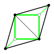
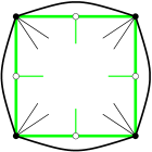
$4$-disk	$8$-disk

Figure 35: The quadrangle of $G$ around a $\{4,8\}$-disk of $A(G)$.

Lemma 23 shows that all the edges of $A(G)$ that are in the interior of a $8$-disk of $A(G)$ and incident to it are entering it. Thus the orientation of the $\{4,8\}$-disk $W^{\prime}$ and of the edges in its interior and incident to it are as depicted on Figure 36. Then by the definition of the mobile $M$ (see rule of Figure 32), there is no half-edge of $M$ in the interior of $Q$ and incident to $Q$. Thus $h_{0}$ is not in $M$. So $h_{0}$ is in the strict interior of $F$ and $F$ is the unique face of $M$. Moreover $M^{+}$ has strictly one more half-edge than $M$.

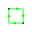
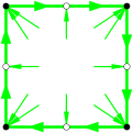
$4$-disk	$8$-disk

Figure 36: Orientation of the $\{4,8\}$-disk.

The number of half-edges of $M$ is equal to $4n$ (one half-edge for each outgoing edge of the $4$-orientation $D_{\min}$ of $A(G)$). Thus the number of half-edges of $M^{+}$ is equal to $4n+1$. The toroidal triangulation $G$ has exactly $3n$ edges. So $M^{+}$ has at least $n+1$ full-edges. Since $M^{+}$ is a graph embedded on the torus with $n$ vertices, if it has strictly more than $n+1$ edges, then it does not have a unique face. So $M^{+}$ has exactly $n+1$ edges and it is a unicellular map covering all the vertices. The number of distinct edges of $G$ covered by $M^{+}$ is exactly $(4n+1)-(n+1)=3n$. So $M^{+}$ is covering all the edges of $G$.

Since there is no half-edge of $M$ in the interior of $Q$ and incident to $Q$. We have that either $W^{\prime}$ is a $4$-disk and $h_{0}$ is a stem of $M^{+}$ or $W^{\prime}$ is a $8$-disk and the removal of $h_{0}$ from $M^{+}$ creates two connected components, one of which is a tree. $\Box$

By Lemma 6, there is a unique maximal quadrangle containing the root half-edge, that we call the root quadrangle.

The example of $K_{7}$ of Figure 33, is an example where the $\{4,8\}$-disk inside the root quadrangle is a $4$-disk. There is no vertices in the strict interior of the root quadrangle and the root half-edge $h_{0}$ of $M^{+}$ (in magenta) is not part of a full-edge of $M^{+}$.

When the root quadrangle has some vertices in its interior, then the $\{4,8\}$-disk inside the root quadrangle is in fact a $8$-disk and the part of the mobile $M$ inside this root quadrangle is a tree (exactly like in the planar case, see [Fus09]). In $M^{+}$ this tree is connected to the “toroidal” part of $M$ that is external to the root quadrangle with the addition of the half-edge $h_{0}$ added to $M^{+}$.

Figure 37 is an example of an essentially $4$-connected toroidal triangulation with some nested quadrangles. The barred half-edge is the root half-edge. It is chosen inside a non empty root quadrangle. There are also non empty quadrangles outside the root quadrangle. The triangulation is given with a balanced transversal structure whose corresponding orientation of the angle graph (not represented) is the minimal balanced $4$-orientation w.r.t. the barred half-edge. The corresponding extended mobile is given. One can see that Theorem 4 is satisfied, i.e. the extended mobile is a unicellular map covering all the vertices and edges. The magenta half-edge, corresponds to the root half-edge and links the two connected part of the mobile, one of which is a tree.

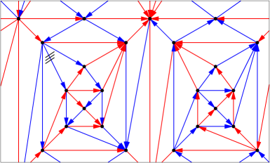
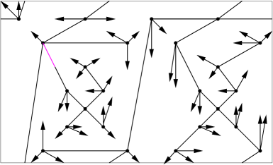
Figure 37: Example of a balanced transversal structure of an essentially $4$-connected toroidal triangulation with some nested quadrangles and the corresponding extended mobile.

A toroidal unicellular map on $n$ vertices has exactly $n+1$ edges. Since the total number of edges of a triangulation on $n$ vertices is $3n$, a consequence of Theorem 4 is that the extended mobile $M^{+}$ has exactly $n$ vertices, $n+1$ edges and $2n-1$ stems. In total, $M^{+}$ has $2(n+1)+2n-1=4n+1$ half-edges. So the root half-edge is not part of the mobile $M$ and is added to $M$ to obtain $M^{+}$. So all the vertices of $M^{+}$ have degree $4$, except the root vertex that has degree $5$.

6.2 Recovering the original triangulation

This section is dedicated to showing how to recover the original triangulation from the extended mobile. The recovering process is described by the following theorem.

Theorem 5

Consider an essentially 4-connected toroidal triangulation $G$, and a root half-edge $h_{0}$ of $G$, incident to a vertex $v_{0}$, such that $h_{0}$ is in the interior and incident to a maximal quadrangle of $G$. From the extended mobile $M^{+}$ associated to the minimal balanced $4$-orientation of $A(G)$ w.r.t. $h_{0}$, one can reattach all the stems of $M^{+}$ to obtain $G$ by starting from the angle of $v_{0}$ just after $h_{0}$ in clockwise order around $v_{0}$ and walking along the face of $M^{+}$ in counterclockwise order (according to the interior of this face): each time a stem is met, it is reattached in order to create a triangular face on its left side.

Theorem 5 is illustrated on Figure 38 to recover $K_{7}$ from the extended mobile of Figure 33. We have represented only the first and last two steps of the method. One can also play with the extended mobile of Figure 37 to recover the corresponding triangulation.

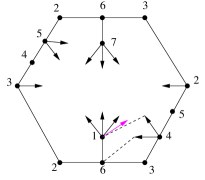
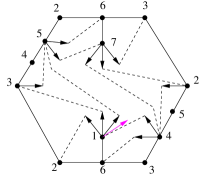
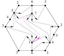
Figure 38: Recovering $K_{7}$ from the extended mobile.

In fact in this section we define a method, more general than the one described in Theorem 5, that is useful for Sections 7.

Let $\mathcal{M}_{r}(n)$ denote the set of toroidal unicellular maps with exactly $n$ vertices, $n+1$ edges and $2n-1$ stems such that all vertices have degree $4$, except one vertex (called root vertex) that has degree $5$, moreover the root vertex has a marked incident half-edge (called the root half-edge) that is either a stem or whose removal creates two connected components, one of which is a tree. Note that the extended mobile $M^{+}$ given by Theorem 4 is an element of $\mathcal{M}_{r}(n)$.

We use the classical closure procedure (see [Fus09]) to reattach step by step all the stems of an element $M^{+}$ of $\mathcal{M}_{r}(n)$. Let $M_{0}=M^{+}$, and, for $1\leq k\leq 2n-1$, let $M_{k}$ be the map obtained from $M_{k-1}$ by reattaching one of its stem (we explicit below which stem is reattached and how). The special face of $M_{0}$ is its only face. For $1\leq k\leq 2n-1$, the special face of $M_{k}$ is the face on the right of the stem of $M_{k-1}$ that is reattached to obtain $M_{k}$. For $0\leq k\leq 2n-1$, the border of the special face of $M_{k}$ consists of a sequence of edges and stems. We define an admissible triple as a sequence $(e_{1},e_{2},s)$, appearing in counterclockwise order along the border of the special face of $M_{k}$, such that $e_{1}=\{u,v\}$ and $e_{2}=\{v,w\}$ are edges of $M_{k}$ and $s$ is a stem attached to $w$. The closure of the admissible triple consists in attaching $s$ to $u$, so that it creates an edge $\{w,u\}$ and so that it creates a triangular face $(u,v,w)$ on its left side (when oriented from $w$ to $u$). The complete closure of $U$ consists in closing a sequence of admissible triples, i.e. for $1\leq k\leq 2n-1$, the map $M_{k}$ is obtained from $M_{k-1}$ by closing any admissible triple.

Note that, for $0\leq k\leq 2n-1$, the special face of $M_{k}$ contains all the stems of $M_{k}$. The closure of a stem reduces the number of edges on the border of the special face and the number of stems by $1$. At the beginning, the unicellular map $M_{0}$ has $n+1$ edges and $2n-1$ stems. So along the border of its special face, there are $2n+2$ edges and $2n-1$ stems. Thus there is exactly three more edges than stems on the border of the special face of $M_{0}$ and this is preserved while closing stems. So at each step there is necessarily at least one admissible triple and the sequence $M_{k}$ is well defined. Since the difference of three is preserved, the special face of $M_{2n-2}$ is a quadrangle with exactly one stem. So the reattachment of the last stem creates two faces that have length three and at the end $M_{2n-1}$ is a toroidal triangulation. Note that at a given step there might be several admissible triples but their closure are independent and the order in which they are performed does not modify the obtained triangulation $M_{2n-1}$.

We now apply the closure method to our particular case. Consider an essentially 4-connected toroidal triangulation $G$, a root half-edge $h_{0}$ of $G$ that is in the interior and incident to a maximal quadrangle of $G$, and the extended mobile $M^{+}$ associated to the minimal balanced $4$-orientation of $A(G)$ w.r.t. $h_{0}$. Recall that $M^{+}$ is an element of $\mathcal{M}_{r}(n)$ so we can apply on $M^{+}$ the complete closure procedure described above. We use the same notation as before, i.e. let $M_{0}=M^{+}$ and for $1\leq k\leq 2n-1$, the map $M_{k}$ is obtained from $M_{k-1}$ by closing any admissible triple. The following lemma shows that the triangulation obtained by this method is $G$:

Lemma 25

The complete closure of $M^{+}$ is $G$, i.e. $M_{2n-1}=G$.

Proof. We prove by induction on $k$ that every face of $M_{k}$ is a face of $G$, except for the special face. This is true for $k=0$ since $M_{0}=M^{+}$ has only one face, the special face. Let $0\leq k\leq 2n-2$, and suppose by induction that every non-special face of $M_{k}$ is a face of $G$. Let $(e_{1},e_{2},s)$ be the admissible triple of $M_{k}$ such that its closure leads to $M_{k+1}$, with $e_{1}=\{u,v\}$ and $e_{2}=\{v,w\}$. The closure of this triple leads to a triangular face $(u,v,w)$ of $M_{k+1}$. This face is the only “new” non-special face while going from $M_{k}$ to $M_{k+1}$.

Suppose, by contradiction, that this face $(u,v,w)$ is not a face of $G$. Let $a_{v}$ (resp. $a_{w}$) be the angle of $M_{k}$ at the special face, between $e_{1}$ and $e_{2}$ (resp. $e_{2}$ and $s$). Since $G$ is a triangulation, and $(u,v,w)$ is not a face of $G$, there exists at least one stem of $M_{k}$ that should be attached to $a_{v}$ or $a_{w}$ to form a proper edge of $G$. Let $s^{\prime}$ be such a stem that is the nearest from $s$. In $G$ the edges corresponding so $s$ and $s^{\prime}$ should be incident to the same triangular face $T$. Let $x$ be the vertex incident to $s^{\prime}$. Let $z\in\{v,w\}$ such that $s^{\prime}$ should be reattached to $z$. If $z=v$, then $s$ should be reattached to $x$ to form a triangular face of $G$. If $z=w$, then $s$ should be reattached to a common neighbor of $w$ and $x$ located on the border of the special face of $M_{k}$ in counterclockwise order between $w$ and $x$. So in both cases $s$ should be reattached to a vertex $y$ located on the border of the special face of $M_{k}$ in counterclockwise order between $w$ and $x$ (with possibly $y=x$). To summarize $s$ goes from $w$ to $y$ and $s^{\prime}$ from $x$ to $z$, and $z,w,y,x$ appear in counterclockwise around $T$ with $z=w$ or $y=x$. The two half-edges $h,h^{\prime}$ of $T$ that are in the same edges with $s,s^{\prime}$ are not in $M^{+}$. By the mobile rule (see Figure 32), the two half-edges $h,h^{\prime}$ that are not in $M^{+}$ corresponds in the orientation of $A(G)$ to two distinct outgoing edges for the dual-vertex corresponding to $T$. This contradicts the fact that the considered orientation of $A(G)$ is a $4$-orientation and that dual-vertices should have outdegree $1$.

So for $0\leq k\leq 2n-2$, all the non-special faces of $M_{k}$ are faces of $G$. In particular every face of $M_{2n-1}$ except one is a face of $G$. Then clearly the (triangular) special face of $M_{2n-1}$ is also a face of $G$, hence $M_{2n-1}=G$. $\Box$

Lemma 25 shows that one can recover the original triangulation from $M^{+}$ with any sequence of admissible triples that are closed successively. This does not explain how to find the admissible triples efficiently. In fact the root half-edge $h_{0}$ can be used to find a particular admissible triple of $M_{k}$. We define the root angle $a_{0}$ of $G$ as the angle of $v_{0}$ just after $h_{0}$ in clockwise order around $v_{0}$. This definition of $a_{0}$ naturally extends to $M^{+}$ or when some admissible triples are reattached.

Lemma 26

For $0\leq k\leq 2n-2$, let $s$ be the first stem met while walking counterclockwise from $a_{0}$ in the special face of $M_{k}$. Then before $s$, at least two edges are met and the last two of these edges form an admissible triple with $s$.

Proof. Since $s$ is the first stem met, there are only edges that are met before $s$. Suppose by contradiction that there is only zero or one edge met before $s$. Then the reattachment of $s$ to form the corresponding edge of $G$ is necessarily such that the triangular face $T$ that is formed on the left side of the stem contains the root half-edge $h_{0}$ on its border. Let $h$ be the half-edge of $T$ that is in the same edge with $s$ and not in $M^{+}$. Then the two half-edges $h,h_{0}$ that are not in $M$ corresponds in the orientation of $A(G)$ to two distinct outgoing edges for the dual-vertex corresponding to $T$. This contradicts the fact that the considered orientation of $A(G)$ is a $4$-orientation and that dual-vertices should have outdegree $1$. $\Box$

Lemma 26 shows that one can reattach all the stems by walking once along the face of $M^{+}$ in counterclockwise order starting from $a_{0}$. Thus we obtain Theorem 5.

Note that $M^{+}$ is such that the complete closure procedure described here never wraps over the root angle, i.e. when a stem is reattached, the root angle is always in the face that is on its right side. The property of never wrapping over the root angle is called safe here. Note that sometimes this property is called “balanced” in the literature and here the word “balanced” is already used with a completely different meaning. Let $\mathcal{M}_{r,s}(n)$ denote the set of elements of $\mathcal{M}_{r}(n)$ that are safe. So the extended mobile given by Theorem 4 is an element of $\mathcal{M}_{r,s}(n)$.

We exhibit in Section 6.4 a bijection between appropriately rooted essentially 4-connected toroidal triangulations and a particular subset of $\mathcal{M}_{r,s}(n)$.

The possibility to close admissible triples in any order to recover the original triangulation is interesting compared to the simpler method of Theorem 5 since it enables to recover the triangulation even if the root half-edge is not given. Indeed, when the root angle is not given, then one can simply start from any angle of $M^{+}$, walk twice around the face of $M^{+}$ in counterclockwise order and reattach all the admissible triples that are encountered along this walk. Walking twice ensures that at least one complete round is done from the root angle. Since only admissible triples are considered, we are sure that no unwanted reattachment is done during the process and that the final map is $G$. This enables us to reconstruct $G$ in linear time even if the root angle is not known. This property will also be used in Section 7 for enumeration purpose.

6.3 Asymptotically optimal encoding

A $4$-connected planar triangulation on $n$ vertices, can be encoded with a binary word of length $\sim n\,\log_{2}(\frac{27}{4})\approx 2.7549\,n$ (see [Fus07, Theorem 4.2]). This is asymptotically optimal since, by results of Tutte, the number $P_{n}$ of $4$-connected planar triangulations on $n$ vertices satisfies $\log_{2}(P_{n})\sim n\,\log_{2}(\frac{27}{4})$. The results of previous sections allow us to generalize this optimal encoding to the toroidal case.

A ternary tree is a plane tree, rooted at a leaf, such that every inner vertex has degree exactly four. A ternary tree $T$ on $n$ inner vertices can easily be encoded using a binary word on $3n$ bits by the following: walk in counterclockwise order around $T$ from the root angle, write a “1” when an inner vertex is discovered for the first time, and a “0” when a leaf is traversed. A ternary tree on $n$ inner vertices has $n$ inner vertices and $2n+2$ leaves. So we obtain a binary word of length $3n+2$ with $n$ bits $1$. Using [BGH03, Lemma 7], this word can then be encoded with a binary word of length $\log_{2}\binom{3n+2}{n}+o(n)\sim n\,\log_{2}(\frac{27}{4})\approx 2.7549\,n$ bits.

Consider an essentially 4-connected toroidal triangulation $G$, a root half-edge $h_{0}$ of $G$ that is in the interior and incident to a maximal quadrangle of $G$, and the extended mobile $M^{+}$ associated to the minimal balanced $4$-orientation of $A(G)$ w.r.t. $h_{0}$. By Theorem 5 one can retrieve the triangulation $G$ from $M^{+}$. Hence to encode $G$, one just has to encode $M^{+}$. The extended mobile $M^{+}$ is a toroidal unicellular map with $n$ vertices, $n+1$ edges, $2n-1$ stems. All its vertices have degree $4$, except the root vertex that has degree $5$. Either $h_{0}$ is a stem of $M^{+}$ or its removal creates two connected components, one of which is a tree.

Let $k\geq 0$ be the number of (inner) vertices of the tree part attached to $h_{0}$, with $k=0$ if $h_{0}$ is a stem. We remove the half-edge $h_{0}$ from $M^{+}$, and obtain : a toroidal component $G_{1}$, that we root at the angle where $h_{0}$ is attached, and a tree component $T_{2}$, that we root at the half-edge opposite to $h_{0}$. So $G_{1}$ is a toroidal unicellular map with $n-k$ vertices, $n-k+1$ edges, $2n-2k-2$ stems. And $T_{2}$ is a planar tree with $k$ vertices, $k-1$ edges, $2k+2$ stems. Moreover, all the vertices of $G_{1}$ and $T_{2}$ have degree $4$. Now we choose two edges $e_{1},e_{2}$ of $G_{1}$, such that $G_{1}\setminus\{e_{1},e_{2}\}$ is acyclic. We transform $G_{1}$ into a planar tree $T_{1}$ by cutting $e_{1},e_{2}$ and transforming each of $e_{1},e_{2}$ into two special stems of $T_{1}$. We root $T_{1}$ on a stem by keeping the information of where are the special stems, which pairs should be reattached together, and where is the angle attached to $h_{0}$. This information can be stored with $O(\log(n))$ bits. One can recover $G_{1}$ from $T_{1}$ by reattaching the special stems in order to form non-contractible cycles and changing the root. Thus we are left to encode two ternary trees $T_{1}$ and $T_{2}$ with $n-k$ and $k$ inner vertices, respectively.

By applying the ternary tree encoding method on $T_{1}$ and $T_{2}$ we obtain the following theorem :

Theorem 6

Any essentially $4$-connected toroidal triangulation on $n$ vertices, can be encoded with a binary word of length $\sim n\,\log_{2}(\frac{27}{4})\approx 2.7549\,n$ and this is asymptotically optimal.

The optimality of Theorem 6 is due to the fact that the number of essentially $4$-connected toroidal triangulations is at least the number of $4$-connected planar triangulations.

Here is a remark on the complexity of the encoding part. All the encoding and decoding process is linear as soon as a balanced transversal structure is given. But even if the proof of Theorem 2 is constructive and gives a polynomial algorithm to find a balanced transversal structure, the obtained algorithm is not linear. The difficulty is to be able to find contractible edges, and contract all the graph to a single vertex, in linear time. Currently this has to be done by Lemma 12 that does not give linear complexity. So the question to be able to find in linear time a balanced transversal structure of an essentially 4-connected triangulation is an interesting and open problem.

In the plane, the proof of the existence of such objects is usually done quite easily by using a so-called shelling order (or canonical order). This method consists in starting from the outer face and removing the vertices one by one. It leads to simple linear time algorithms. We do not see how to generalize this kind of method here since the toroidal objects that we considered are too homogeneous and there is no special face (and thus no particular starting point) playing the role of the outer face.

6.4 Bijective consequences

Consider an essentially 4-connected toroidal triangulation $G$, a root half-edge $h_{0}$ of $G$ that is in the interior and incident to a maximal quadrangle, and the extended mobile $M^{+}$ associated to the minimal balanced $4$-orientation of $A(G)$ w.r.t. $h_{0}$. Theorems 4 and 5 show that $M^{+}$ gives a toroidal unicellular map with stems from which one can recover the original triangulation. Thus there is a bijection between essentially 4-connected toroidal triangulations rooted from an appropriate half-edge and their corresponding set of extended mobiles. The goal of this section is to describe exactly the set of these extended mobiles.

Recall from Section 6.2 that the obtained extended mobiles are elements of $\mathcal{M}_{r,s}(n)$. One may hope that there is a bijection between essentially 4-connected toroidal triangulations appropriately rooted and $\mathcal{M}_{r,s}(n)$. This is the classic behavior in the planar case since there is a unique lattice associated to the set of $\alpha$-orientations of a planar map (for a fixed $\alpha$). But here, things are different since the set of $4$-orientations of the angle map is now partitioned into several lattices and there might be several minimal elements, some of which behave well w.r.t. the mobile rule. Indeed, there exists examples of minimal non-balanced $4$-orientations of angle maps of essentially 4-connected toroidal triangulations appropriately rooted such that the corresponding extended mobile is in $\mathcal{M}_{r,s}(n)$. The balanced property is the property that defines uniquely our considered minimal element and thus we have to translate this property on the set of mobiles.

Note that there are two types of toroidal unicellular maps. Two cycles of a unicellular map may intersect either on a single vertex (square case) or on a path (hexagon case). We call such maps square unicellular maps or hexagon unicellular maps, respectively. The square can be seen as a particular case of the hexagon where one side has length zero and thus the two corners of the hexagon are identified. In the square case (resp. hexagon case), the unicellular map has exactly $2$ (resp. $3$) distinct cycles that are moreover non-contractible and not weakly homologous to each other.

Recall that given a cycle $C$ of $G$ with a direction of traversal, we have $\gamma(C)$ equals the number of edges of $A(G)$ leaving $C$ on its right minus the number of edges of $A(G)$ leaving $C$ on its left. Recall that the root angle of $G$ is the angle just after the root half-edge in clockwise order. In each angle of the extended mobile $M^{+}$, except the root angle, there is an outgoing edge of $A(G)$ (see rule of Figure 32). So for a cycle $C$ of the extended mobile, one can compute $\gamma(C)$ by considering the angles of $M^{+}$ on the left and right side of $C$, except the root angle. Then, since we are considering balanced $4$-orientations of the angle map, for any (non-contractible) cycle $C$ of the extended mobile obtained by Theorem 4, we have $\gamma(C)=0$.

Consider an element $M^{+}$ of $\mathcal{M}_{r}(n)$. We say that an unicellular map of $\mathcal{M}_{r}(n)$ is balanced if every cycle of the unicellular map has the same number of angles on the left and right sides, with the special rule that the root angle does not count. Let $\mathcal{M}_{r,s,b}(n)$ denote the subset of elements of $\mathcal{M}_{r,s}(n)$ that are balanced.

Let us recall, for the sake of clarity, the complete definition of $\mathcal{M}_{r,s,b}(n)$ that is the set of toroidal unicellular maps with exactly $n$ vertices, $n+1$ edges and $2n-1$ stems such that:

• “r” for root: All vertices have degree $4$, except one vertex (called root vertex) that has degree $5$, moreover the root vertex has a marked incident half-edge (called the root half-edge) that is either a stem or whose removal creates two connected components, one of which is a tree.

• “s” for safe: When the stems of admissible triples are reattached (in any order), the angle just after the root half-edge in clockwise order (called the root angle) is always in the face that is on the right side of the stems.

• “b” for balanced: Every (non-contractible) cycle of the map has the same number of angles on its left and right sides, with the special rule that the root angle does not count.

Let $\mathcal{T}_{r}(n)$ be the set of essentially 4-connected toroidal triangulations on $n$ vertices rooted at a half-edge that is in the interior and incident to a maximal quadrangle.

We have the following bijection:

Theorem 7

There is a bijection between $\mathcal{T}_{r}(n)$ and $\mathcal{M}_{r,s,b}(n)$.

Proof. Consider the mapping $g$ that associates to an element of $\mathcal{T}_{r}(n)$, the extended mobile $M^{+}$ obtained by Theorem 4. By the above discussion the image of $g$ is in $\mathcal{M}_{r,s,b}(n)$ and $g$ is injective since one can recover the original triangulation from its image by Theorem 5.

Conversely, given an element $M^{+}$ of $\mathcal{M}_{r,s,b}(n)$ with root angle $a_{0}$ (just after the root half-edge in clockwise order around the root vertex), one can build a toroidal map $G$ by the complete closure procedure described in Section 6.2. The number of stems and edges of $M^{+}$ implies that all faces of $G$ are triangles. We explain later why $G$ has no contractible loop nor multiple edges and that it is essentially 4-connected.

While making the complete closure, one can create a 4-orientation $D$ of $A(G)$ with the following method. For each half-edge $h$ of $M^{+}$ distinct from $h_{0}$, such that $h$ is incident to vertex $v$, add to $D$ an outgoing half-edge incident to $v$ and just after $h$ in clockwise order around $v$. Note that this is done not only for stems of $M^{+}$ but for all the half-edges of $M^{+}$, including those that are part of full-edges of $M^{+}$, except $h_{0}$.

Consider the moment when an admissible triple $(e_{1},e_{2},s)$ of $M_{k}$ is closed in order to obtain $M_{k+1}$, with $0\leq k\leq 2n-2$. Let $e_{1}=(u,v)$, $e_{2}=(v,w)$ and $s$ is a stem attached to $w$. When the stem $s$ is reattached to $u$ to form a triangular face $T$ on its left side, it is reattached to $u$ in order to leave the half-edge of $D$ leaving $u$ (if any) on the right side (see Figure 39). Note that if the angle at $u$ is the root angle, then there is no half-edge of $D$ leaving $u$. By doing so we maintain the property that for all the angles of the face containing the root angle (called the special face in Section 6.2), there is an outgoing half-edge of $D$, except for the root angle.

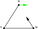
Figure 39: Reattachment of a stem.

In order to describe the edges of $D$ completely, we consider two cases whether $s$ is the last stem that is reattached or not.

• $s$ is not the last reattached stem

  By the safe property, $s$ has the root angle on its right side when it is reattached. So the angle at $v$ (resp. $w$) between $e_{1},e_{2}$ (resp. $e_{2},s$) in clockwise order is not the root angle. So inside the triangle $T$, we can reattached the two half-edges of $D$ incident to $v,w$ to the dual-vertex $f$ of $A(G)$ corresponding to $T$ and add an additional edge to $D$ from $f$ to $u$ (see Figure 40).

  

  

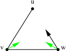
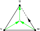
  Figure 40: Reattachment of a stem and orientation of the angle map.

• $s$ is the last reattached stem

  By the safe property, the root angle is in the face on the right side of $s$. Thus we are in one of the three case of Figure 41 depending on the position of the root half-edge according to $s$ (the root half-edge is represented in magenta). In each case we reattached the four depicted half-edges of $D$ and add two additional edges to $D$ that are outgoing for dual-vertices of $D$ as described on Figure 41.

  

  

  

  

  

  

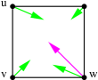
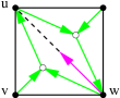
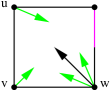
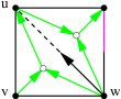
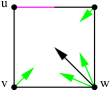
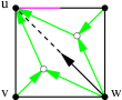
  Figure 41: The three possible cases for the reattachment of the last stem.

By doing so we are sure to reattach all the half-edges of $D$ to dual-vertices of $A(G)$. In the end, all primal-vertices have outdegree $4$ and all dual-vertices have outdegree $1$. So we have defined a $4$-orientation $D$ of $A(G)$ on which the mobile rule (see Figure 32) plus the addition of the root half-edge gives $M^{+}$. Since we are considering a 4-orientation of $A(G)$, the map $G$ has no contractible loop nor multiple edges and it is essentially 4-connected, otherwise, there will be a contradiction in a region homeomorphic to an open disk by a simple counting argument. It remains to show that $G$ is appropriately rooted and that $D$ corresponds to the minimal balanced $4$-orientation w.r.t. this root, then $g$ will be surjective.

Since $M^{+}$ is balanced it has at least two non-contractible and not weakly homologous cycles $C_{1},C_{2}$ with the same number of angles on their respective left and right sides, with the special rule that the root angle does not count. All these angles corresponds to exactly one outgoing edge of $D$ by construction of $D$. So the orientation $D$ of $A(G)$ satisfies $\gamma(C_{1})=\gamma(C_{2})=0$. So by Lemma 14, the 4-orientation $D$ is balanced.

Suppose by contradiction that $D$ is not minimal w.r.t. $h_{0}$. Let $f_{0}$ be the face of $A(G)$ containing $h_{0}$. We use the terminology and notations of Section 5.2. Then in the Hasse diagram of the lattice $(\mathcal{B}(A(G)),\leq_{f_{0}})$, there is an element below $D$: Let $D^{\prime}$ be a balanced $4$-orientation of $A(G)$ such that $D^{\prime}\leq_{f_{0}}D$. By Section 5.2, we have $D^{\prime}\setminus D\in\widetilde{\mathcal{F}}^{\prime}$. Let $\widetilde{F}=D^{\prime}\setminus D$. So $\widetilde{F}$ is the counterclockwise facial walk of a face of $\widetilde{A(G)}$ not containing $f_{0}$. So this facial walk is oriented counterclockwise (resp. clockwise) according to its interior in $D^{\prime}$ (resp. $D$). By Lemma 22, $\widetilde{F}$ is quasi-contractible and its outer facial walk is a $\{4,8\}$-disk $W$. Then, by Lemma 23, if $W$ is a 8-disk, the edges that are in the interior of $W$ and incident to it are entering it. So in $D$, the orientation of $W$ and of the edges in its interior and incident to it are as depicted on Figure 36. Then, by definition of the mobile (see Figure 32), there is no half-edge of $M^{+}$ in the interior of $W$ and incident to vertices of $W$. If $W$ is a $\{4\}$-disk, then the unique edge of $G$ inside $W$ is not covered by $M^{+}$. If $W$ is a $\{8\}$-disk, then either there are some edges of $G$ inside $W$ that are not covered by $M^{+}$, or $M^{+}$ is made of several connected components. In any cases, this contradicts the fact that $M^{+}$ is an element of $\mathcal{M}_{r,s,b}(n)$ from which $G$ is obtained by applying the complete closure procedure. So $D$ is minimal w.r.t. $h_{0}$, and thus it is the minimal balanced $4$-orientation w.r.t. $h_{0}$

Suppose by contradiction that $h_{0}$ is not “in the interior and incident” to a maximal quadrangle. Then by Lemma 6, there is a unique maximal quadrangle $Q$ whose interior contains $h_{0}$. Since $h_{0}$ is not “in the interior and incident” to $Q$, it is in the strict interior of $Q$. The quadrangle $Q$ corresponds to a $\{4,8\}$-disk $W$ of $A(G)$ (see Figure 35). Note that $W$ is a maximal $\{4,8\}$-disk containing $h_{0}$. So, by Lemma 24, in $D$, the $\{4,8\}$-disk $W$ is oriented clockwise w.r.t. its interior. It is not possible that $W$ is a $4$-disk since then $h_{0}$ is not in the strict interior of $Q$ but incident to it. So $W$ is a $8$-disk. By Lemma 23, the edges that are in the interior of $W$ and incident to it are entering it. Then the orientation of $W$ and of the edges in its interior and incident to it are as depicted on Figure 36. Then by the definition of the mobile (see rule of Figure 32), there is no half-edge of $M^{+}$ in the interior of $Q$ and incident to $Q$. So either there are some edges of $G$ that are not covered by $M^{+}$, or $M^{+}$ is made of several connected components. In both cases, this contradicts the fact that $M^{+}$ is an element of $\mathcal{M}_{r,s,b}(n)$ from which $G$ is obtained by applying the complete closure procedure. So $h_{0}$ is in the interior and incident to a maximal quadrangle of $G$. $\Box$

7 Counting essentially 4-connected toroidal triangulations

Let $\mathcal{T}_{h}(n)$ be the set of essentially 4-connected toroidal triangulations on $n$ vertices, rooted at any half-edge. In this section we show how to count $\mathcal{T}_{h}(n)$ (see Theorem 8). The first values of $|\mathcal{T}_{h}(n)|$, for $n\geq 0$, are $0,1,6,40,268,1801,12120$ (sequence A289208 in OEIS [Slo]). Figure 42 illustrates the six elements of $\mathcal{T}_{h}(2)$.

Figure 42: The six elements of $\mathcal{T}_{h}(2)$: two different underlying graphs, each with three possible roots represented by an outgoing half-edge.

7.1 Decomposition into planar and toroidal parts

Consider an element of $\mathcal{T}_{h}(n)$. Recall that by Lemma 6, there is a unique maximal quadrangle containing the root half-edge, that we call the root quadrangle. We define the corners of a quadrangle of a map as the four angles that appear in the interior of this quadrangle when its interior is removed (if non empty). We define $\mathcal{T}_{h,c}(n)$ as the set of elements of $\mathcal{T}_{h}(n)$ with a marked corner of the root quadrangle. The elements of $\mathcal{T}_{h,c}$ are decomposed into the toroidal part that is outside the root quadrangle and the planar part that is in the interior of the root quadrangle.

We first need the following lemma, which shows that removing the interior of the root quadrangle does not change the connectivity of the remaining part. Even if the statement has nothing to do with transversal structures, the proof is using them as in Section 2.3.

Lemma 27

If $G$ is an essentially 4-connected toroidal triangulations given with a maximal quadrangle $Q$, then the map $G^{\prime}$ obtained by removing all the vertices and edges that lie in the interior of $Q$ is an essentially 4-connected toroidal map.

Proof. Let $G$ be an essentially 4-connected toroidal triangulations given with a maximal quadrangle $Q$ and $G^{\prime}$ obtained by removing all the vertices and edges that lie in the interior of $Q$.

Consider a root half-edge $h_{0}$ of $G$ that is in the interior and incident to $Q$. Consider the minimal balanced $4$-orientation $D_{\min}$ of $A(G)$ w.r.t. $h_{0}$. By Corollary 1, this $4$-orientation corresponds to a transversal structure of $G$. Consider the $\{4,8\}$-disk $W$ of $A(G)$ that is inside the maximal quadrangle $Q$. By Lemma 24, in $D_{\min}$, the $\{4,8\}$-disk $W$ is oriented clockwise w.r.t. its interior. Lemma 23 shows that all the edges of $A(G)$ that are in the interior of a $8$-disk of $A(G)$ and incident to it are entering it. So the transversal structure of $G$ represented on the maximal quadrangle $Q$ is as depicted on one of the three cases of Figure 43 (where the outer edges represent the quadrangle $Q$).

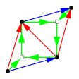
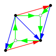
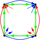
Figure 43: Transversal structure on the maximal quadrangle $Q$.

Recall that from Section 2.3, that for a vertex $v$ of $G^{\infty}$, the subgraph $P_{0}(v)$ (resp. $P_{1}(v)$, $P_{2}(v)$, $P_{3}(v)$) of $G^{\infty}$ is obtained by keeping all the edges that are on an oriented path of $G^{\infty}_{B}$ (resp. $G^{\infty}_{R}$, $(G^{\infty}_{B})^{-1}$, $(G^{\infty}_{R})^{-1}$) starting at $v$. By Lemma 2, the subgraphs $P_{i}(v)$ are acyclic. Let $P^{\prime}_{i}(v)$ be defined similarly but in $G^{\prime\infty}$. So $P^{\prime}_{i}(v)$ is a subgraph of $P_{i}(v)$, thus it is also acyclic. Note that removing the interior of the quadrangle $Q$ on the three cases of Figure 43, does not change the fact that around every vertex there are edges that are outgoing blue, outgoing red, incoming blue and incoming red. So the $P^{\prime}_{i}(v)$ are infinite.

As in the proof of Lemma 4, suppose by contradiction that there exists three vertices $x,y,z$ of $G^{\prime\infty}$ such that $G^{\prime\prime}=G^{\prime\infty}\setminus\{x,y,z\}$ is not connected. Then, by Lemma 1, the graph $G^{\prime\prime}$ has a finite connected component $R$. Let $v$ be a vertex of $R$. For $i\in\{0,1,2,3\}$, the infinite and acyclic graph $P^{\prime}_{i}(v)$ does not lie in $R$ so it intersects one of $x,y,z$. So for two distinct $i,j$, the two graphs $P^{\prime}_{i}(v)$ and $P^{\prime}_{j}(v)$ intersect in a vertex distinct from $v$. Thus the two graphs $P_{i}(v)$ and $P_{j}(v)$ intersect in a vertex distinct from $v$, a contradiction to Lemma 3. $\Box$

Let $\mathcal{T}_{c}^{t}(n)$ be the set of essentially 4-connected toroidal maps on $n$ vertices, where all faces are triangles, except one that is a maximal quadrangle, and, with a marked corner of this quadrangle. In particular we have $|\mathcal{T}_{c}^{t}(0)|=0$ and $|\mathcal{T}_{c}^{t}(1)|=1$.

Let $\mathcal{T}_{h,c}^{p}(n)$ be the set of 4-connected planar maps on $n$ inner vertices, where all faces are triangles, except the outer-face that is a quadrangle, with a marked corner of this quadrangle, and rooted at an inner half-edge. Note that here, $n$ counts the number of inner vertices, so there are $n+4$ vertices in an element of $\mathcal{T}_{h,c}^{p}(n)$. In particular we have $|\mathcal{T}_{h,c}^{p}(0)|=4$ and $|\mathcal{T}_{h,c}^{p}(1)|=8$.

Then we have the following bijection:

Lemma 28

There is a bijection between $\mathcal{T}_{h}(n)\times\{1,2,3,4\}$ and $\bigcup_{1\leq k\leq n}(\mathcal{T}_{h,c}^{p}(n-k)\times\mathcal{T}_{c}^{t}(k))$.

Proof. By Lemma 6, there is a bijection between $\mathcal{T}_{h}(n)\times\{1,2,3,4\}$ and $\mathcal{T}_{h,c}(n)$. By Lemma 27, there is a bijection between $\mathcal{T}_{h,c}(n)$ and $\bigcup_{1\leq k\leq n}(\mathcal{T}_{h,c}^{p}(n-k)\times\mathcal{T}_{c}^{t}(k))$. The composition of these two bijections gives the result. $\Box$

By Lemma 28, the enumeration of the elements of $\mathcal{T}_{h}$ is reduced to the enumeration of their planar part $\mathcal{T}_{h,c}^{p}$ and their toroidal part $\mathcal{T}_{c}^{t}$.

Recall from Section 6.3, that a ternary tree is a plane tree, rooted at a leaf, such that every inner vertex has degree exactly four. For $n\geq 1$, let $\mathcal{A}(n)$ denote the set of ternary trees with $n$ inner vertices. By convention we consider that the tree composed of a single vertex is the unique element of $\mathcal{A}(0)$. The associated generating function satisfies:

$$A(z)=\sum_{n}|\mathcal{A}(n)|z^{n}=1+zA(z)^{3}.$$ (1)

The enumeration of $\mathcal{T}_{h,c}^{p}$ is given by the following lemma:

Lemma 29

$$|\mathcal{T}_{h,c}^{p}(n)|=\frac{4}{n+1}\binom{3n+1}{n}$$

and the associate generating function satisfies:

$$T_{h,c}^{p}(z)=\sum_{n\geq 0}|\mathcal{T}_{h,c}^{p}(n)|z^{n}=4A(z)^{2}.$$

Proof. [Fus09, Theorem 3] is a bijection between the set $\mathcal{P}(n)$ of (unrooted) plane tree such that every inner vertex has degree exactly four and the set $\mathcal{T}^{p}(n)$ of (unrooted) 4-connected planar maps on $n$ inner vertices, where all faces are triangles, except the outer-face that is a quadrangle.

Let $\mathcal{T}_{h}^{p}(n)$ be the set of elements of $\mathcal{T}^{p}(n)$ rooted at an inner half-edge. Let $\mathcal{P}_{o}(n)$ be the elements of $\mathcal{P}(n)$ with one oriented edge. In the bijection of [Fus09, Theorem 3], each inner edge of the map corresponds to an edge of the corresponding tree. So rooting the elements of $\mathcal{T}^{p}(n)$ on a particular inner half-edge, corresponds to orienting an edge of the tree. Thus we have a bijection between $\mathcal{T}_{h}^{p}(n)$ and $\mathcal{P}_{o}(n)$.

Cutting an element of $\mathcal{P}_{o}(n)$ at the oriented edge creates bijectively a couple of ternary trees with respectively $k$ and $n-k$ inner vertices, with $0\leq k\leq n$. Hence:

$$P_{o}(z)=\sum_{n}|\mathcal{P}_{o}(n)|=A(z)^{2}.$$

As shown in [GX06, p 11], the coefficients of $A(z)^{2}$ admit a simple expression:

$$|\mathcal{P}_{o}(n)|=\frac{1}{n+1}\binom{3n+1}{n}.$$

An element of $\mathcal{T}_{h,c}^{p}(n)$ is obtained from an element of $\mathcal{T}_{h}^{p}(n)$ by marking one corner of the outer face. There are four such choice so $\mathcal{T}_{h,c}^{p}(n)=4\mathcal{T}_{h}^{p}(n)=4\mathcal{P}_{o}(n)$ and we obtain the lemma. $\Box$

7.2 Bijection with square and hexagonal unicellular maps

Given an element $M^{+}$ of $\mathcal{M}_{r,s,b}(n)$ (see Section 6.4 for the definition), we define the unrooted mobile $M$ associated to $M^{+}$ as the toroidal unicellular map obtained from $M^{+}$ by removing the root half-edge and the tree part attached to the root half-edge (if any). Figure 44 gives the unrooted mobile associated to the extended mobile of Figure 37.

Figure 44: The unrooted mobile obtained from the extended mobile of Figure 37.

Let $\mathcal{M}_{b}(n)$ denote the set of (non-rooted) toroidal unicellular maps with exactly $n$ vertices, $n+1$ edges and $2n-2$ stems such that all vertices have degree $4$, and every cycle of the map has the same number of angles on its left and right sides (balanced property).

Consider an element $M^{+}$ of $\mathcal{M}_{r,s,b}(n)$. Let $k\geq 0$ be the number of vertices in the tree part attached to the root half-edge (if any), with $k=0$ if the root half-edge is a stem. Then one can see that the unrooted mobile $M$ associated to $M^{+}$ is an element of $\mathcal{M}_{b}(n-k)$.

Consider an element $M$ of $\mathcal{M}_{b}(n)$. A mobile-labeling of $M$ is a labeling $\ell$ of the half-edges of $M$ with integers $0,1,2,3$ such that the labels that appear around each vertex are exactly $0,1,2,3$ in counterclockwise order and the two labels that appear on each edge differ exactly by $(2\bmod 4)$, see right of Figure 34 for an example. Let $G$ be the graph obtained from $M$ by closing all its admissible triples. Since, $M$ has $2n-2$ stems, we have that $G$ is a “toroidal triangulation minus one edge”, i.e. a toroidal map whose all faces are triangles except one that is a quadrangle. The extension of $\ell$ to $G$ is the labeling of all the half-edges of $G$ obtained from $\ell$ by keeping the property that the two labels that appear on each edge differs exactly by $2\bmod 4$. Next lemma shows that the quadrangle of $G$ is labeled as on Figure 45 in the extension of the mobile-labeling.

Figure 45: Labeling of the remaining quadrangle after extending a mobile-labeling.

Each angle of $M$ corresponds to consecutive angles of $G$ (reattaching a stem into an angle, splits this angle in two). Conversely, to each angle of $G$ we can associate the unique corresponding angle of $M$ from which it comes from. Then we have the following:

Lemma 30

Consider an element $M$ of $\mathcal{M}_{b}(n)$ given with a particular angle $\alpha$. Then $M$ admits a unique mobile-labeling, noted $\ell(\alpha)$, such that the angle $\alpha$ is between half-edges labeled $0$ and $1$. Moreover, after closing the admissible triples of $M$ to obtain $G$, the extension of $\ell(\alpha)$ to $G$ is such that the quadrangle $Q$ of $G$ is labeled as on Figure 45. And the four angles of $M$ that corresponds to the angles of $Q$ are incident to half-edges with exactly the same labels in $M$ and in $Q$.

Proof. The toroidal unicellular map $M$ has $n$ vertices, $n+1$ edges and $2n-2$ stems such that all vertices have degree $4$, and every cycle of the map has the same number of angles on its left and right sides.

Let $h$ be the half-edge of $M$ that is incident to $\alpha$ and just after $\alpha$ in clockwise order around its incident vertex. Let $\ell(\alpha)$ be the labeling of the half-edges of $M$ with integers $0,1,2,3$ obtained by the following: Label $h$ with $0$ and then extend the labeling to all the half-edges of $M$ by keeping the property that the labels that appear around each vertex are exactly $0,1,2,3$ in counterclockwise order and the two labels that appear on each edge differ exactly by $(2\bmod 4)$. This is possible and consistent since every cycle of the map has the same number of angles on its left and right sides. Indeed, given a cycle $C$ of length $k$, there are $2k$ angles on each sides, so the modification of the labels while starting from a half-edge of $C$, walking along $C$ and going back to the starting half-edge is the following: the number of edges of $C$ times $(2\bmod 4)$, i.e. $(2k\bmod 4)$, plus the number of angles on the right side of $C$, i.e. $(2k\bmod 4)$, so $(4k\bmod 4)=0$ in total. Thus, this definition of the mobile-labeling $\ell(\alpha)$ is consistent and moreover it is the unique such labeling. So we have the first part of the lemma.

Let $M_{0}=M$. For $1\leq k\leq 2n-2$, let $M_{k}$ be the map obtained from $M_{k-1}$ by closing an admissible triple of $M_{k-1}$. Extend the labeling $\ell(\alpha)$ while closing admissible triples by keeping the property that the two labels that appear on each edge differs exactly by $2\bmod 4$. We prove by induction on $k$, that each map $M_{k}$, for $0\leq k\leq 2n-2$, satisfies the following: each angle of the special face of $M_{k}$ is between half-edges whose labels are distinct (and precisely the same as for the corresponding angle of $M_{k-1}$ if $k\geq 1$), moreover the labels that appear in counterclockwise order around each vertex of $M_{k}$ form four non-empty intervals of $0,1,2,3$. Indeed, $M_{0}$ satisfies the property and suppose that for $1\leq k\leq 2n-2$, we have $M_{k-1}$ that satisfies the property. Consider the admissible triple $(e_{1},e_{2},s)$ of $M_{k-1}$ that is closed to obtain $M_{k}$. Let $e_{1}=\{u,v\}$ and $e_{2}=\{v,w\}$ with $s$ is a stem attached to $w$. Let $i\in\{0,1,2,3\}$ such that $s$ is labeled $i$. Then since $M_{k-1}$ satisfies the property on the labels we have that:

• the half-edge of $e_{2}$ incident to $w$ is labeled $(i+1)\bmod 4$

• the half-edge of $e_{2}$ incident to $v$ is labeled $(i+3)\bmod 4$

• the half-edge of $e_{1}$ incident to $v$ is labeled $i$

• the half-edge $h_{u}$ of $e_{1}$ incident to $u$ is labeled $(i+2)\bmod 4$

• the half-edge $h^{\prime}_{u}$ incident to $u$ and just after $h_{u}$ in counterclockwise order around $u$ is labeled $(i+3)\bmod 4$

When the admissible triple is closed, a half-edge $h_{s}$, opposite to $s$ is created and receive the label $(i+2)\bmod 4$. So the half-edges $h_{u},h_{s},h^{\prime}_{u}$ appear consecutively in counterclockwise order around $u$. Moreover they are labeled $(i+2)\bmod 4$, $(i+2)\bmod 4$ and $(i+3)\bmod 4$ respectively. So all the induction properties are preserved. Finally, $M_{2n-2}$ satisfies the property and its special face, that is a quadrangle, is labeled as on Figure 45 and the four angles of $M$ that corresponds to the angles of $Q$ are incident to half-edges with exactly the same labels in $M$ and in $Q$. $\Box$

Recall that there are two types of toroidal unicellular maps. Two distinct cycles of a toroidal unicellular map may intersect either on a single vertex (square case) or on a path (hexagon case). In a square (resp. hexagon) unicellular map, there are exactly $2$ (resp. $3$) distinct cycles. A vertex of a toroidal unicellular map is called special if is contained in all the cycles of the map. Note that there is exactly one special vertex in a square unicellular map, and exactly two special vertices in a hexagon unicellular map.

Let $\mathcal{M}^{s}_{b}(n)$ (resp. $\mathcal{M}^{h}_{b}(n)$) denote the set of elements of $\mathcal{M}_{b}(n)$ that are square (resp. hexagon) unicellular maps. Moreover we denote the sets $\mathcal{M}_{b,a}(n),\mathcal{M}^{s}_{b,a}(n),\mathcal{M}^{h}_{b,a}(n)$ the sets of elements of $M_{b}(n),\mathcal{M}^{s}_{b}(n),\mathcal{M}^{h}_{b}(n)$, respectively, that are rooted at an angle of a special vertex.

We have the following bijection:

Lemma 31

There is a bijection between $\mathcal{T}_{c}^{t}(n)\times\{1,2\}$ and $\mathcal{(}M^{s}_{b,a}(n)\times\{1,2\})\cup(\mathcal{M}^{h}_{b,a}(n)\times\{0\})$.

Proof. We define a bijective function from $\mathcal{T}_{c}^{t}(n)\times\{1,2\}$ to $(\mathcal{M}^{s}_{b,a}(n)\times\{1,2\})\cup(\mathcal{M}^{h}_{b,a}(n)\times\{0\})$. This function is defined via three intermediate functions $a$, $g^{\prime}$ and $r$ defined below.

Let $a$ (for “add”) be the mapping defined on the elements $G$ of $\mathcal{T}_{c}^{t}(n)$ that adds to $G$ a diagonal $e_{0}$ in the interior of the (maximal) quadrangle $Q$ of $G$, incident to the marked corner $\alpha$ of $Q$, and returns the obtained map $Z$ rooted at the half-edge $h_{0}$ of $e_{0}$ incident to $\alpha$. Let $\mathcal{T}^{\prime}_{r}(n)$ be the subset of $\mathcal{T}_{r}(n)$ (see definition in Section 6.4) such that the two faces incident to the root half-edge form a maximal quadrangle. We claim the following:

Claim 3

$a$ is a bijection from $\mathcal{T}_{c}^{t}(n)$ to $\mathcal{T}^{\prime}_{r}(n)$.

Proof.  Let $G$ be an element of $\mathcal{T}_{c}^{t}(n)$ and $Z$ its image by $a$. Consider the notations of the definition of $a$. Since $G$ is essentially 4-connected, the added edge $e_{0}$ cannot create a contractible loop in $Z$. If adding $e_{0}$ creates a pair of homotopic multiple edges in $Z$ with an edge $e^{\prime}_{0}$, then there are two edges of the quadrangle $Q$ of $G$ plus edge $e^{\prime}_{0}$ that form a separating triangle of $G^{\infty}$ contradicting the $4$-connectedness of $G^{\infty}$. So the obtained map $Z$ is a toroidal triangulation with no contractible loop nor homotopic multiple edges. Moreover since $Q$ is a maximal quadrangle, the edge $e_{0}$ cannot create a separating triangle of $Z^{\infty}$. So by Lemma 5, the toroidal triangulation $Z$ is essentially $4$-connected. Moreover $Z$ has the particularity that the two faces incident to the root half-edge $h_{0}$ form a maximal quadrangle of $Z$. So $Z$ is is in $\mathcal{T}^{\prime}_{r}(n)$.

Let $\overline{a}$ be the mapping defined on the elements $Z$ of $\mathcal{T}^{\prime}_{r}(n)$ that removes from $Z$ the edge containing the root half-edge and mark the obtained quadrangle at the corner incident to $h_{0}$. Then clearly $\overline{a}\circ a=Id$.

Conversely, let $Z$ be an element of $\mathcal{T}^{\prime}_{r}(n)$ and consider its image $G$ by $\overline{a}$. We have $Z$ is an essentially 4-connected toroidal triangulation on $n$ vertices rooted at a half-edge that is in the interior and incident to a maximal quadrangle, and such that the two faces incident to the root half-edge form a maximal quadrangle. So $G$ is a toroidal map on $n$ vertices, where all faces are triangles, except one that is a maximal quadrangle and with a marked corner of this quadrangle. The map $G$ is obtained from $Z$ by removing the interior of a maximal quadrangle so, by Lemma 27, $G$ is essentially 4-connected. So $G$ is in $\mathcal{T}_{c}^{t}(n)$.

We clearly have $a\circ\overline{a}=Id$. So $a$ is a bijection from $\mathcal{T}_{c}^{t}(n)$ to $\mathcal{T}^{\prime}_{r}(n)$. $\Diamond$

Let $g^{\prime}$ be the restriction of the bijection $g$, defined in the proof of Theorem 7, to the elements of $\mathcal{T}^{\prime}_{r}(n)$. Let $\mathcal{M}^{\prime}_{r,s,b}(n)$ be the subset of $\mathcal{M}_{r,s,b}(n)$ (see definition in Section 6.4) such that the root half-edge is a stem. We claim the following:

Claim 4

$g^{\prime}$ is a bijection from $\mathcal{T}^{\prime}_{r}(n)$ to $\mathcal{M}^{\prime}_{r,s,b}(n)$.

Proof.  Let $Z$ be an element of $\mathcal{T}^{\prime}_{r}(n)$ and $M^{+}\in\mathcal{M}_{r,s,b}(n)$ its image by $g$. By definition of $\mathcal{T}^{\prime}_{r}(n)$, the two faces incident to the root half-edge $h_{0}$ form a maximal quadrangle $Q$. In the minimal balanced $4$-orientation of $A(Z)$ w.r.t. $h_{0}$, the $4$-disk $W$ inside $Q$ is oriented clockwise by Lemma 24 (see left of Figure 36). Then by the definition of the mobile (see rule of Figure 32), there is no half-edge of $M^{+}$ in the interior of $Q$ except $h_{0}$. So $h_{0}$ is a stem of $M^{+}$. So $M^{+}$ is in $\mathcal{M}^{\prime}_{r,s,b}(n)$.

Let $\overline{g^{\prime}}$ be the restriction of $g^{-1}$ to the elements of $\mathcal{M}^{\prime}_{r,s,b}(n)$. Since $g$ is a bijection, we have $\overline{g^{\prime}}\circ g^{\prime}=Id$.

Conversely, let $M^{+}$ be an element of $\mathcal{M}^{\prime}_{r,s,b}(n)$ and consider its image $Z$ by $g^{-1}$. By the proof of Theorem 7, the complete closure procedure on $M^{+}$ gives an essentially 4-connected toroidal triangulation $Z$ of $\mathcal{T}_{r}(n)$ rooted at $h_{0}$ and such that $h_{0}$ is in the interior and incident to a maximal quadrangle $Q^{\prime}$. Moreover, $M^{+}$ is the extended mobile associated to the minimal balanced 4-orientation $D_{\min}$ of $A(Z)$ w.r.t. $h_{0}$. The quadrangle $Q^{\prime}$ corresponds to a $\{4,8\}$-disk $W$ of $A(Z)$ (see Figure 35). Note that $W$ is a maximal $\{4,8\}$-disk containing $h_{0}$. So, by Lemma 24, $W$ is oriented clockwise w.r.t. its interior in $D_{\min}$. Then, by Lemma 23, the orientation of $W$ and of the edges in its interior and incident to it are as depicted on Figure 36. Then by the definition of the mobile (see rule of Figure 32), there is no half-edge of $M^{+}$, distinct from $h_{0}$, in the interior of $Q^{\prime}$ and incident to $Q^{\prime}$. Since $M^{+}$ is covering all the edges of $Z$, we have that $Q^{\prime}$ has no edges in its interior, except the one containing $h_{0}$. So $Q^{\prime}$ is the quadrangle formed by the two faces incident to $h_{0}$. So the two faces incident to $h_{0}$ form a maximal quadrangle and so $Z$ is an element of $\mathcal{T}^{\prime}_{r}(n)$.

Since $g$ is a bijection, we have $g^{\prime}\circ\overline{g^{\prime}}=Id$. So $g^{\prime}$ is a bijection from $\mathcal{T}^{\prime}_{r}(n)$ to $\mathcal{M}^{\prime}_{r,s,b}(n)$. $\Diamond$

Let $r$ (for “remove”) be the mapping defined on the elements $(M^{+},x)$ of $\mathcal{M}^{\prime}_{r,s,b}(n)\times\{1,2\}$, that removes the root half-edge $h_{0}$ of $M^{+}$ that is a stem and roots the obtained mobile $M$ at an angle of a special vertex by the following rule. Let $\alpha$ be the angle of $M$ such that $M^{+}$ is obtained from $M$ by adding $h_{0}$ in the angle $\alpha$. Consider the unique mobile-labeling $\ell(\alpha)$ of $M$, given by Lemma 30. If $M$ is square, let $\beta$ be the angle of the special vertex of $M$ that is between the half-edges labeled $0$ and $1$. In this case, $r$ returns $(M,x)$ rooted at $\beta$. If $M$ is hexagon, let $v_{1}$ (resp. $v_{2}$) be the first (resp. second) special vertex of $M$ that is encountered while walking counterclockwise along the border of the unique face of $M$, starting from $\alpha$. For $i\in\{1,2\}$, let $\beta_{i}$ be the angle of $v_{i}$ that is between half-edges labeled $0$ and $1$. In this case, $r$ returns $(M,0)$ rooted at $\beta_{x}$. We claim the following:

Claim 5

$r$ is a bijection from $\mathcal{M}^{\prime}_{r,s,b}(n)\times\{1,2\}$ to $(\mathcal{M}^{s}_{b,a}(n)\times\{1,2\})\cup(\mathcal{M}^{h}_{b,a}(n)\times\{0\})$.

Proof.  It is clear by the definition of $r$ that the image by $r$ of an element of $\mathcal{M}^{\prime}_{r,s,b}(n)\times\{1,2\}$ is in $(\mathcal{M}^{s}_{b,a}(n)\times\{1,2\})\cup(\mathcal{M}^{h}_{b,a}(n)\times\{0\})$.

Let $\overline{r}$ be the mapping defined on the elements $(M,y)$ of $(\mathcal{M}^{s}_{b,a}(n)\times\{1,2\})\cup(\mathcal{M}^{h}_{b,a}(n)\times\{0\})$ by the following. Let $\beta$ be the root angle of $M$ and consider the unique labeling $\ell(\beta)$ of $M$, given by Lemma 30. Close all the admissible triples of $M$ to obtain a map $G$ whose special face is a quadrangle $Q$. Propagate the labeling $\ell(\beta)$ to $G$ by keeping the property that the two labels that appear on an edge has to differ exactly by $(2\bmod 4)$. Then by Lemma 30 the quadrangle $Q$ of $G$ is labeled as on Figure 45. So $Q$ has a unique angle $\alpha$ between half-edges labeled $0$ and $1$. We also denote $\alpha$ the angle of $M$ that corresponds to the angle $\alpha$ of $Q$. Let $M^{+}$ be the map obtained from $M$ by forgetting its root angle $\beta$ and adding a root half-edge $h_{0}$ incident to $\alpha$. If $M$ is square, then let $x=y$. If $M$ is hexagon, let $x$ be such that $\beta$ is an angle incident to the $x$-th special vertex of $M$ encountered while walking counterclockwise along the face of $M$, starting from $\alpha$. Then $\overline{r}$ returns $(M^{+},x)$.

We claim that:

(1) $\overline{r}\circ r=Id$

Let $(M^{+},x)$ be an element of $\mathcal{M}^{\prime}_{r,s,b}(n)\times\{1,2\}$ and $(M,y)$ its image by $r$. We use the notation of the definition of $r$, i.e. the map $M$ is obtained from $M^{+}$ by removing the root half-edge $h_{0}$ of $M^{+}$, incident to the angle $\alpha$ of $M$ and rooting $M$ according to the labeling $\ell(\alpha)$ at an angle $\beta$ between half-edges labeled $0$ and $1$. By Lemma 30, there is a unique mobile-labeling of $M$ such that $\beta$ is between half-edges labeled $0$ and $1$. So the labeling $\ell(\beta)$ used in the definition of $\overline{r}$ is exactly the same as $\ell(\alpha)$. So $M^{+}$ is obtained from $M$ by adding a half-edge $h_{0}$ at an angle between half-edges labeled $0$ and $1$ of $\ell(\beta)$.

From $M^{+}$, one can build the graph $Z=g^{-1}(M^{+})\in\mathcal{T}^{\prime}_{r}(n)$ by closing admissible triples in any order. The recovering method of Theorem 5 says that the root half-edge $h_{0}$ can be the last stem that is reattached by this procedure. So the graph $G$ defined in the definition of $\overline{r}$ is obtained from $Z$ by removing the edge containing the root half-edge. So $M^{+}$ is obtained from $M$ by adding a half-edge $h_{0}$ at an angle of $M$ corresponding to one of the angle of the quadrangle $Q$ of $G$.

By Lemma 30, the extension of the labeling $\ell(\beta)$ to $G$ shows that the quadrangle $Q$ of $G$, is labeled as on Figure 45. Moreover the angles of $M$ that corresponds to the angles of $Q$ are incident to half-edges with exactly the same labels in $M$ and in $Q$. So there is a unique such angle $\alpha$ of $M$ between half-edges labeled $0$ and $1$. So $M^{+}$ is obtained from $M$ by adding a half-edge $h_{0}$ at the angle of $M$ corresponding to $\alpha$ and $\overline{r}\circ r=Id$.

This proves (1).

Conversely, let $(M,y)$ be an element of $(\mathcal{M}^{s}_{b,a}(n)\times\{1,2\})\cup(\mathcal{M}^{h}_{b,a}(n)\times\{0\})$ and $(M^{+},x)$ its image by $\overline{r}$. Since $M$ is balanced, we have that $M^{+}$ is also balanced. Moreover, the root half-edge $h_{0}$ is added to $M$ in an angle of the special face obtained after reattaching all the admissible triples of $M$. So $M^{+}$ is safe and $(M^{+},x)$ is in $\mathcal{M}^{\prime}_{r,s,b}(n)\times\{1,2\}$.

It is clear that $r\circ\overline{r}=Id$, so $r$ is a bijection. $\Diamond$

By Claim 3 to 5, we have $r\circ(g^{\prime},Id)\circ(a,Id)$ is a bijection from $\mathcal{T}_{c}^{t}(n)\times\{1,2\}$ to $(\mathcal{M}^{s}_{b,a}(n)\times\{1,2\})\cup(\mathcal{M}^{h}_{b,a}(n)\times\{0\})$. $\Box$

7.3 Enumeration of skeletons

A skeleton is a toroidal unicellular map such that every inner vertex, i.e. every vertex of degree at least two, belongs to its cycles. A skeleton is balanced if every cycle of the map has the same number of angles on its left and right sides. A skeleton is square (resp. hexagon) if it is a square (resp. hexagon) unicellular map. Let $\mathcal{S}_{a}(n)$ be the set of skeletons on $n$ inner vertices, such that all inner vertices have degree $4$, and rooted at an angle of a special vertex. Let $\mathcal{S}_{b,a}(n)$ be the set of balanced element of $\mathcal{S}_{a}(n)$. Let $\mathcal{S}_{a}^{s}(n)$, $\mathcal{S}_{a}^{h}(n)$, $\mathcal{S}_{b,a}^{s}(n)$ and $\mathcal{S}_{b,a}^{h}(n)$ be the sets of square and hexagon elements of $\mathcal{S}_{a}(n)$ and $\mathcal{S}_{b,a}(n)$, respectively.

Given an element $M$ of $\mathcal{M}_{b}(n)$, the skeleton of $M$ is obtained from $M$ by removing all the vertices that are not vertices of the cycles of $M$ nor in their neighborhood. It is direct to see that the skeletons of elements of $\mathcal{M}_{b,a}(n)$ are in $\mathcal{S}_{b,a}(n)$.

An element of $\mathcal{M}_{b,a}(n)$ can be uniquely decomposed into an element of $\mathcal{S}_{b,a}(k)$, for some $k\geq 1$, and a $(2k-2)$-uplet of ternary trees (each ternary tree being attached to a leaf of the skeleton) such that the total number of inner vertices of the trees is $n-k$.

Let $\mathcal{F}(n,k)$ be the set of $k$-uplets of rooted ternary trees with total number of inner vertices $n$. Its associated generating function satisfies $F(z,u)=\sum_{n,k}|\mathcal{F}(n,k)|z^{n}u^{k}=\sum_{k}A(z)^{k}u^{k}=\frac{1}{1-uA(z)}$. Moreover, it is known that $|\mathcal{F}(n,k)|=\frac{k}{2n-k}\binom{3n-k-1}{n}$ (see [Sta99, Theorem 5.3.10]).

Let $S^{s}_{b,a}$ and $S^{h}_{b,a}$ be the generating functions associated to $\mathcal{S}^{s}_{b,a}$ and $\mathcal{S}^{h}_{b,a}$, respectively, i.e. $S^{s}_{b,a}(z)=\sum_{n}|\mathcal{S}^{s}_{b,a}(n)|z^{n}$ and $S^{h}_{b,a}(z)=\sum_{n}|\mathcal{S}^{h}_{b,a}(n)|z^{n}$.

Then we have the following lemma:

Lemma 32

$$|\mathcal{M}_{b,a}^{s}(n)|=\sum_{k=1}^{n}|\mathcal{S}_{b,a}^{s}(k)|.|\mathcal{F}(n-k,2k-2)|$$

$$|\mathcal{M}_{b,a}^{h}(n)|=\sum_{k=1}^{n}|\mathcal{S}_{b,a}^{h}(k)|.|\mathcal{F}(n-k,2k-2)|$$

and the associated generating functions satisfy:

$$M^{s}_{b,a}(z)=\sum_{n\geq 1}|\mathcal{M}^{s}_{b,a}(n)|z^{n}=S^{s}_{b,a}(zA(z)^{2})/A(z)^{2}$$

$$M^{h}_{b,a}(z)=\sum_{n\geq 1}|\mathcal{M}^{h}_{b,a}(n)|z^{n}=S^{h}_{b,a}(zA(z)^{2})/A(z)^{2}.$$

Proof. The first two formulas are clear by above decomposition. Moreover, each element of $\mathcal{M}_{b,a}^{s}(n)$ is obtained by substituting each of the $2k-2$ leaves of an element of $\mathcal{S}_{b,a}^{s}(k)$ by a ternary tree. So we have:

$$M^{s}_{b,a}(z) = \sum_{k\geq 1}|\mathcal{S}_{b,a}^{s}(k)|A(z)^{2k-2}z^{k}$$

$$= \frac{1}{A(z)^{2}}\sum_{k\geq 1}|\mathcal{S}_{b,a}^{s}(k)|(A(z)^{2}z)^{k}$$

$$= \frac{S^{s}_{b,a}(zA(z)^{2})}{A(z)^{2}}.$$

Similarly, we have $M^{h}_{b,a}(z)=\frac{S^{h}_{b,a}(zA(z)^{2})}{A(z)^{2}}$. $\Box$

By Lemma 32, we are reduced to the enumeration of $\mathcal{S}_{b,a}^{s}$ and $\mathcal{S}_{b,a}^{h}$.

Consider an element $S$ of $\mathcal{S}_{a}(n)$. If $S$ is square, consider the two edge-disjoint closed walks of $S$ started from the special vertex, noted $W_{1}$ and $W_{2}$. We assume that $W_{1}$ and $W_{2}$ are chosen such that the two half-edges $h_{1},h_{2}$ that are incident to the root angle of $S$ are traversed from the special vertex in $W_{1}$, $W_{2}$, respectively, and that $h_{1}$ and $h_{2}$ appear consecutively in counterclockwise order around the special vertex. If $S$ is hexagon, then consider the three walks $W_{1}$, $W_{2}$ and $W_{3}$ of $S$ starting from the special vertex $v_{1}$ containing the root angle, ending at the second special vertex $v_{2}$, such that the three paths $W_{1},W_{2},W_{3}$ appears consecutively in counterclockwise order around $v_{1}$, starting from the leaf attached to $v_{1}$. Note that, for the square or hexagonal case, the $W_{i}$ are uniquely defined and oriented. Along each walk $W_{i}$, the inner vertices that are encountered may have both leaves on the right, both leaves on the left, or one leaf on each side. In next two lemmas, we encode this by using Grand Motzkin prefix/paths defined below.

A Grand Motzkin prefix (or GM prefix for short) of length $n$, is a path in $\mathbb{Z}^{2}$, starting at the point $(0,0)$, ending at the point $(n,\delta)$, with $\delta\in\mathbb{Z}$, and composed of $k$ steps $(1,1)$, $(1,-1)$ and $(1,0)$. Let $gm(n,\delta)$ be the number of GM prefix of length $n$ starting at $(0,0)$ and ending at $(n,\delta)$ and $GM(z,u)=\sum_{n,\delta}gm(n,\delta)z^{n}u^{\delta}$. There is one GM prefix of length $0$ and a GM prefix of length $n>0$ is obtained by adding one step $(1,1)$, $(1,-1)$ or $(1,0)$ to a GM prefix of length $(n-1)$. This decomposition leads to the following equation:

$$GM(z,u)=1+z(u+1/u+1)GM(z,u)=\frac{1}{1-z(u+1/u+1)}=\sum_{n\geq 0}(1+1/u+u)^{n}z^{n}.$$

Let $[z^{n}]f$ denote the coefficient of $z^{n}$ of function $f(z)$, i.e. if $f=\sum_{n}f_{n}z^{n}$ then $[z^{n}]=f_{n}$.

A Grand Motzkin path (or GM path for short) of length $k$ is a Grand Motzkin prefix of length $k$, ending at the point $(k,0)$. The generating function associated to GM paths satisfies $GM(z)=[u^{0}]GM(z,u)=\frac{1}{\sqrt{1-2z-3z^{2}}}$ (see [FM14]).

The square skeletons satisfy:

Lemma 33

$$|\mathcal{S}_{b,a}^{s}(n)|=\frac{3^{n}-(-1)^{n}}{4}$$

$$S^{s}_{b,a}(z)=\frac{z}{1-2z-3z^{2}}.$$

Proof. With above notations, an element of $\mathcal{S}_{b,a}^{s}(n)$ is uniquely decomposed into a special vertex and the two closed walks $W_{1}$ and $W_{2}$. for $i\in\{1,2\}$, let $r_{i}$ (resp. $l_{i}$) be the number of leaves of $S$ incident to an inner vertex of $W_{i}$ that are on the right (resp. left) side of $W_{i}$. Let $\delta_{i}=(r_{i}-l_{i})/2$. Since the special node as no leaves attached to it, the balanced property implies that $\delta_{1}=\delta_{2}=0$. So if $W_{i}$ contains $k_{i}$ inner vertices, then $W_{i}$ can be encoded by a GM path of length $k_{i}$. This decomposition results in the product of respective generating series: $S^{s}_{b,a}(z)=z.GM(z)^{2}=\frac{z}{1-2z-3z^{2}}$.

Now observe that $S^{s}_{b,a}(z)-2zS^{s}_{b,a}(z)-3z^{2}S^{s}_{b,a}(z)=z$. We deduce the following recurrence: for $n\geq 2$, we have $|\mathcal{S}_{b,a}^{s}(n)|=2|\mathcal{S}_{b,a}^{s}(n-1)|+3|\mathcal{S}_{b,a}^{s}(n-2)|$. Moreover, we have $|\mathcal{S}_{b,a}^{s}(0)|=0$ and $|\mathcal{S}_{b,a}^{s}(1)|=1$. Since $\frac{3^{n}-(-1)^{n}}{4}$ satisfies the same conditions $|\mathcal{S}_{b,a}^{s}(n)|$, the two are identical. $\Box$

The hexagon skeletons satisfy:

Lemma 34

$$|\mathcal{S}_{b,a}^{h}(n)|=(n-2).3^{n-1}+\frac{5.3^{n-1}+(-1)^{n}}{4}$$

$$S^{h}_{b,a}(z)=\frac{4z^{2}}{(z+1)(3z-1)^{2}}.$$

Proof. Let $S$ be an element of $\mathcal{S}_{a}^{h}(n)$. Note that $S$ is not assumed to be balanced here. Considering this larger class, we are able extract the series $S^{h}_{b,a}(z)$ by following the standard diagonal method [Sta99, Section 6.3]. As with above notations, consider the three walks $W_{1}$, $W_{2}$ and $W_{3}$ of $S$ starting from the special vertex $v_{1}$ containing the root angle, ending at the second special vertex $v_{2}$, such that the three paths $W_{1},W_{2},W_{3}$ appear consecutively in counterclockwise order around $v_{1}$, starting from the leaf attached to $v_{1}$.

There are different cases to consider depending on the position of the leaves. We say that $S$ is of Type $i$ if the leaf of $v_{2}$ is after $W_{i}$ in the counterclockwise order around $v_{2}$ (see the top line of Figure 46). In order to ease the upcoming computation, let rename these walks depending of the type. For types 1 and 3, let $W_{c}=W_{1},W_{x}=-W_{2}$ and $W_{y}=-W_{3}$ (see the bottom left and bottom right of Figure 46). For type 2, let $W_{c}=W_{3},W_{x}=-W_{1}$ and $W_{y}=-W_{2}$ (see the bottom center of Figure 46, where edges have been redrawn differently than in top-center figure).

Type 1	Type 2	Type 3

Figure 46: Different types of hexagon skeletons.

Let $C_{1},C_{2}$ be the cycles of $S$ made of $W_{c}+W_{x}$ and $W_{c}+W_{y}$ respectively, with the direction of traversal corresponding to the orientation of $W_{c},W_{x},W_{y}$. For $i\in\{1,2\}$, let $\delta_{i}$ be the number of leaves of $S$ incident to $C_{i}$ that are on its right side minus the number of leaves of $S$ incident to $C_{i}$ that are on its left side, divided by two.

Let $\mathcal{S}_{a}^{h}(k,\ell,n)$ denote the elements of $\mathcal{S}_{a}^{h}(n)$ such that $\delta_{1}=k$ and $\delta_{2}=\ell$, with $(k,\ell)\in\mathbb{Z}^{2}$. Let $S^{h}_{a}(u,v,z)$ be the associated generating function, i.e. $S^{h}_{a}(u,v,z)=\sum_{(k,\ell,n)\in\mathbb{Z}^{2}\times\mathbb{N}}|\mathcal{S}_{a}^{h}(k,\ell,n)|u^{k}v^{\ell}z^{n}$. This generating function can be computed with the following method. An hexagonal skeleton can be decomposed into 2 special vertices (contributing for $z^{2}$) plus tetra-valent caterpillars $C_{c}$, $C_{x}$ and $C_{y}$ respectively contributing for $GM(z,uv)$, $GM(z,u)$ and $GM(z,v)$. Depending of the type of hexagon skeleton, the special vertices are contributing for $+1$, $0$ or $-1$ to $\delta_{1}$ and $\delta_{2}$, this is translated by a factor $(\frac{1}{uv}+uv+1)$ on the generating function. There are four possible root angles around $v_{1}$, so we have:

$$S^{h}_{a}(u,v,z) = 4z^{2}(uv+\frac{1}{uv}+1)(GM(z,uv).GM(z,u).GM(z,v))$$

$$= -\frac{4z^{2}(u^{2}v^{2}+uv+1)uv}{(u^{2}z+uz-u+z)(v^{2}z+vz-v+z)(u^{2}v^{2}z+uvz-uv+z)}.$$

Observe that $S^{h}_{b,a}(z)=[v^{0}][u^{0}]S^{h}_{a}(u,v,z)$.

The denominator of $S^{h}_{a}(u,v,z)$, seen as a polynomial of $u$ admits four roots: $U,\frac{1}{U},\frac{U}{v}$ and $\frac{1}{Uv}$ where $U=\frac{1-z-\sqrt{-3z^{2}-2z+1}}{2z}$, and we have:

$$S^{h}_{a}(u,v,z)=-\frac{4(u^{2}v^{2}+uv+1)u}{(u-U)(u-\frac{1}{U})(u-\frac{U}{v})(u-\frac{1}{Uv})v(v^{2}z+vz-v+z)}.$$

Hence $S^{h}_{a}(u,v,z)$ can be converted into partial fractions of $u$:

$$S^{h}_{a}(u,v,z)=A.\biggl{(} \frac{U^{2}+Uv+v^{2}}{(1-Uu)U^{2}v^{2}(U^{2}-v)}+\frac{U^{2}v^{2}+Uv+1}{(1-\frac{U}{u})uUv^{2}(1-U^{2}v)}$$

$$+\frac{U^{2}+U+1}{(1-\frac{U}{uv})(U^{2}-v)Uuv^{2}}+\frac{U^{2}+U+1}{(1-Uuv)U^{2}v(1-U^{2}v)}\biggl{)},$$

where $A=\frac{4v^{3}U^{3}}{(v-1)(U^{2}-1)(v^{2}z+vz-v+z)}$.

As $A=\mathcal{O}(z^{3})$ and $U=\mathcal{O}(z)$ (when $z$ tends to $0$), this identity splits into a sum of four power series in $z$ with coefficients in $\mathbb{Q}[u,\frac{1}{u},v,\frac{1}{v}]$, two with only negative powers of $u$ and two with only nonnegative powers of $u$.

$$S^{h}_{a}(u,v,z)=A.\biggl{(} \frac{U^{2}+Uv+v^{2}}{U^{2}v^{2}(U^{2}-v)}\sum_{n\geq 0}(Uu)^{n}+\frac{U^{2}v^{2}+Uv+1}{uUv^{2}(1-U^{2}v)}\sum_{n\geq 0}\left(\frac{U}{u}\right)^{n}$$

$$+\frac{U^{2}+U+1}{(U^{2}-v)Uuv^{2}}\sum_{n\geq 0}\left(\frac{U}{uv}\right)^{n}+\frac{U^{2}+U+1}{U^{2}v(1-U^{2}v)}\sum_{n\geq 0}\left(Uuv\right)^{n}\biggl{)}.$$

Hence the coefficient $[u^{0}]$ can be directly extracted:

$$[u^{0}]S^{h}_{a}(u,v,z) = A.\left(\frac{U^{2}+Uv+v^{2}}{U^{2}v^{2}(U^{2}-v)}+\frac{U^{2}+U+1}{U^{2}v(1-U^{2}v)}\right)$$

$$= \frac{4(v^{2}z+vz+v+z)z^{2}v}{\sqrt{-(z+1)(3z-1)}(v^{2}z^{2}+vz^{2}+2vz+z^{2}-v)(v^{2}z+vz-v+z)}.$$

Again, the denominator of $[u^{0}]S^{h}_{a}(u,v,z)$, seen as a polynomial of $v$ admits four roots: $V_{0},\frac{1}{V_{0}},V_{1},\frac{1}{V_{1}}$ where $V_{0}=U$ and $V_{1}=-\frac{z^{2}+\sqrt{-(z+1)(3z-1)}(1-z)+2z-1}{2z^{2}}$.

Hence $[u^{0}]S^{h}_{a}(u,v,z)$ can be converted into partial fractions of $v$:

$$[u^{0}]S^{h}_{a}(u,v,z)=B.\biggl{(} \frac{V_{0}(V_{0}^{2}z+V_{0}z+V_{0}+z)}{(1-V_{0}/v)v(V_{0}^{2}-1)(V_{0}V_{1}-1)}+\frac{V_{1}(V_{1}^{2}z+V_{1}z+V_{1}+z)}{(1-V_{1}/v)v(-V_{1}^{2}+1)(V_{0}V_{1}-1)}$$

$$+\frac{V_{0}^{2}z+V_{0}z+V_{0}+z}{(1-V_{0}v)(V_{0}^{2}-1)(V_{0}V_{1}-1)}+\frac{V_{1}^{2}z+V_{1}z+V_{1}+z}{(1-V_{1}v)(1-V_{1}^{2})(V_{0}V_{1}-1)}\biggl{)},$$

where $B=\frac{4V_{0}V1}{z\,\sqrt{-(z+1)(3z-1)}(V_{0}-V_{1})}$.

As $B=\mathcal{O}(z)$, $V_{0}=\mathcal{O}(z)$ and $V_{1}=\mathcal{O}(z^{2})$, this identity splits into a sum of four power series in $z$ with coefficients in $\mathbb{Q}[v,\frac{1}{v}]$, two with only negative powers of $v$ and two with only nonnegative powers of $v$.

$$[u^{0}]S^{h}_{a}(u,v,z)=B.\biggl{(} \frac{V_{0}(V_{0}^{2}z+V_{0}z+V_{0}+z)}{v(V_{0}^{2}-1)(V_{0}V_{1}-1)}\sum_{n\geq 0}\left(\frac{V_{0}}{v}\right)^{n}+\frac{V_{1}(V_{1}^{2}z+V_{1}z+V_{1}+z)}{v(-V_{1}^{2}+1)(V_{0}V_{1}-1)}\sum_{n\geq 0}\left(\frac{V_{1}}{v}\right)^{n}$$

$$+\frac{V_{0}^{2}z+V_{0}z+V_{0}+z}{(V_{0}^{2}-1)(V_{0}V_{1}-1)}\sum_{n\geq 0}\left(V_{0}v\right)^{n}+\frac{V_{1}^{2}z+V_{1}z+V_{1}+z}{(1-V_{1}^{2})(V_{0}V_{1}-1)}\sum_{n\geq 0}\left(V_{1}v\right)^{n}\biggl{)},$$

Hence the coefficient $[v^{0}]$ can be directly extracted:

$$[v^{0}][u^{0}]S^{h}_{a}(u,v,z)=B\left(\frac{V_{0}^{2}z+V_{0}z+V_{0}+z}{(V_{0}^{2}-1)(V_{0}V_{1}-1)}+\frac{V_{1}^{2}z+V_{1}z+V_{1}+z}{(V_{1}^{2}-1)(V_{0}V_{1}-1)}\right).$$

Which simplifies into the second part of the lemma:

$$S^{h}_{b,a}(z)=[v^{0}][u^{0}]S^{h}_{a}(u,v,z)=\frac{4z^{2}}{(z+1)(3z-1)^{2}}.$$

We can observe that $S^{h}_{b,a}(z)-5zS^{h}_{b,a}(z)+3z^{2}S^{h}_{b,a}(z)+9z^{3}S^{h}_{b,a}(z)=4z$. We deduce the following recurrence for $n>3$, $|\mathcal{S}_{b,a}^{h}(n)|=5|\mathcal{S}_{b,a}^{h}(n-1)|-3|\mathcal{S}_{b,a}^{h}(n-2)|-9|\mathcal{S}_{b,a}^{h}(n-3)|$. Moreover, we have $|\mathcal{S}_{b,a}^{h}(0)|=|\mathcal{S}_{b,a}^{h}(1)|=0$ and $|\mathcal{S}_{b,a}^{h}(2)|=4$. Since $(n-2).3^{n-1}+\frac{5.3^{n-1}+(-1)^{n}}{4}$ satisfies the same conditions as $|\mathcal{S}_{b,a}^{h}(n)|$, the two are identical.

$\Box$

7.4 Enumeration theorem

The enumeration theorem that we obtain is the following:

Theorem 8

The generating function associated to the number $\mathcal{T}_{h}(n)$ of essentially 4-connected toroidal triangulations on $n$ vertices, rooted on any half-edge, is:

$$T_{h}(z)=\sum_{n\geq 0}|\mathcal{T}_{h}(n)|z^{n}=\frac{zA(z)}{7zA(z)^{2}-21zA(z)+9z+1}$$

where $A(z)$ is the generating function of (leaf-rooted) ternary trees satisfying $A(z)=1+zA(z)^{3}$.

Moreover, the values of $|\mathcal{T}_{h}(n)|$ are given by the following formulas:

$$|\mathcal{T}_{h}(n)|=\frac{1}{4}\sum_{k=1}^{n}|\mathcal{T}_{h,c}^{p}(n-k)|.|\mathcal{T}_{c}^{t}(k)|$$

$$|\mathcal{T}_{h,c}^{p}(n)|=\frac{4}{n+1}\binom{3n+1}{n}$$

$$|\mathcal{T}_{c}^{t}(n)|=\sum_{k=1}^{n}\mathcal{S}(k).|\mathcal{F}(n-k,2k-2)|$$

$$\mathcal{S}(n)=\frac{(-1)^{n-1}+(3+4n)3^{n-1}}{8}$$

$$|\mathcal{F}(n,k)|=\frac{k}{2n-k}\binom{3n-k-1}{n}.$$

Proof. By Lemma 28, we have:

$$|\mathcal{T}_{h}(n)|=\frac{1}{4}\sum_{k=0}^{n}|\mathcal{T}_{h,c}^{p}(n-k)|.|\mathcal{T}_{c}^{t}(k)|$$

and so:

$$T_{h}(z)=\frac{1}{4}T_{h,c}^{p}(z)T_{c}^{t}(z).$$ (2)

By Lemma 29, we have:

$$|\mathcal{T}_{h,c}^{p}(n)|=\frac{4}{n+1}\binom{3n+1}{n}$$

$$T_{h,c}^{p}(z)=4A(z)^{2}.$$ (3)

By Lemma 31, we have:

$$|\mathcal{T}_{c}^{t}(n)|=|\mathcal{M}^{s}_{b,a}(n)|+\frac{1}{2}|\mathcal{M}^{h}_{b,a}(n)|$$ (4)

$$T_{c}^{t}(z)=M^{s}_{b,a}(z)+\frac{1}{2}M^{h}_{b,a}(z).$$ (5)

Let $\mathcal{S}(n)=|\mathcal{S}_{b,a}^{s}(n)|+\frac{1}{2}|\mathcal{S}_{b,a}^{h}(n)|$ and $S(z)=S^{s}_{b,a}(z)+\frac{1}{2}S^{h}_{b,a}(z)$. So, by Lemma 32, Equations (4) and (5) become:

$$|\mathcal{T}_{c}^{t}(n)|=\sum_{k=1}^{n}\mathcal{S}(k).|\mathcal{F}(n-k,2k-2)|$$

$$T_{c}^{t}(z)=\frac{S(zA(z)^{2})}{A(z)^{2}}.$$ (6)

From Lemmas 33 and 34, we obtain:

$$\mathcal{S}(n)=\frac{(-1)^{n-1}+(3+4n)3^{n-1}}{8}$$

$$S(z)=\frac{z(1-z)}{(1+z)(1-3z)^{2}}.$$ (7)

From (6) and (7), we obtain:

$$T_{c}^{t}(z)=\frac{z-z^{2}.A(z)^{2}}{(z.A(z)^{2}+1).(3z.A(z)^{2}-1)^{2}}.$$ (8)

Combining (2), (3) and (8) gives :

$$T_{h}(z)=\frac{(z-z^{2}A(z)^{2})A(z)^{2}}{(zA(z)^{2}+1)(3zA(z)^{2}-1)^{2}}.$$

By (1) (see Section 7.1), one can replace $zA^{3}$ by $A-1$ in above formula and obtain:

$$T_{h}(z)=\frac{zA(z)}{7zA(z)^{2}-21zA(z)+9z+1}.$$

$\Box$

Part of the proof of Theorem 8 relies on generating function analysis and do not completely explain the simplicity of some expressions. For instance, sequences of the number of different kinds of skeletons ($S^{s}_{b,a}(n)$ and $S^{h}_{b,a}(n)$) have nice simple formulas (see Lemmas 33 and 34) that deserve clean bijective interpretations. Note that these sequences already appear in OEIS [Slo] (resp. A015518, A191008). Having a bijective proof of the enumeration of skeletons could be essential to provide an efficient (e.g. sub-quadratic) random generation algorithm for essentially $4$-connected toroidal maps.

8 Conclusion

In this paper, we have generalized transversal structures and some of its applications to the toroidal case. Using only a local property in the definition, as in the planar case, is not enough to obtain interesting properties. Indeed, the set of toroidal transversal structures of a given toroidal map is partitioned into several distributive lattices. The main point of this paper is to be able to find a global property, called “balanced”, that such an object may have or may not have. Then, the set of balanced objects defines a unique lattice whose minimal element has properties useful to apply techniques devised for the planar case. This is very similar to what happens for Schnyder woods for which it is also possible to define an analogous balanced property (see [Lév17]). Then, one can apply on these minimal balanced objects, the “mobile method” as here, or alternatively “Poulalhon and Schaeffer’s method” as in [DGL17], to obtain bijections between the considered classes of toroidal maps and particular toroidal unicellular maps. This seems to be a general framework that can be applied to various classes of toroidal maps and their corresponding set of $\alpha$-orientations. In a paper to come of Eric Fusy and the second author, a similar balanced property is found for toroidal fractional $\frac{d}{d-2}$-orientations with similar bijective consequences. A challenging question is to see if one can go further and found a generalization of the balanced property in higher genus. Currently we have no idea of what could be the answer even for the double torus.

Schnyder woods and transversal structures are also used in the planar case to compute straightline grid drawings of plane triangulations [Sch89, Fus09]. Recently toroidal Schnyder woods have been used to obtain drawings of toroidal graphs (see [GL14]). Another natural application of toroidal transversal structures would be a straightline grid drawing algorithm of essentially 4-connected toroidal triangulations.

Acknowledgments. We would like to thank Mireille Bousquet-Mélou, Eric Fusy and Daniel Gonçalves for fruitful discussions and suggestions.

References

- [BC11] Olivier Bernardi and Guillaume Chapuy. A bijection for covered maps, or a shortcut between harer–zagier’s and jackson’s formulas. Journal of Combinatorial Theory, Series A, 118(6):1718–1748, 2011.
- [BF12a] Olivier Bernardi and Eric Fusy. A bijection for triangulations, quadrangulations, pentagulations, etc. Journal of Combinatorial Theory, Series A, 119(1):218–244, 2012.
- [BF12b] Olivier Bernardi and Eric Fusy. Unified bijections for maps with prescribed degrees and girth. Journal of Combinatorial Theory, Series A, 119(6):1351 – 1387, 2012.
- [BGH03] N. Bonichon, C. Gavoille, and N. Hanusse. An information-theoretic upper bound of planar graphs using triangulation. In Annual Symposium on Theoretical Aspects of Computer Science (STACS), volume 2607 of Lecture Notes in Computer Science, pages 499–510. Springer-Verlag, February 2003.
- [Cha11] G. Chapuy. A new combinatorial identity for unicellular maps, via a direct bijective approach. Advances in Applied Mathematics, 2011.
- [CMS09] G. Chapuy, M. Marcus, and G. Schaeffer. A bijection for rooted maps on orientable surfaces. SIAM Journal on Discrete Mathematics, 2009.
- [DGL17] Vincent Despré, Daniel Gonçalves, and Benjamin Lévêque. Encoding toroidal triangulations. Discrete and Computational Geometry, 57:507–544, 2017.
- [dM94] P. Ossona de Mendez. Orientations bipolaires. PhD thesis, 1994.
- [Fel04] S. Felsner. Lattice structures from planar graphs. Electronic Journal of Combinatorics, 2004.
- [FM14] Luca Ferrari and Emanuele Munarini. Enumeration of edges in some lattices of paths. Journal of Integer Sequences, 17(2):3, 2014.
- [Fus07] Eric Fusy. Combinatoire des cartes planaires et applications algorithmiques. PhD thesis, 2007.
- [Fus09] Éric Fusy. Transversal structures on triangulations: A combinatorial study and straight-line drawings. Discrete Mathematics, 309(7):1870–1894, 2009.
- [GKL16] Daniel Gonçalves, Kolja B. Knauer, and Benjamin Lévêque. On the structure of schnyder woods on orientable surfaces. arXiv:1501.05475v2, 2016.
- [GL14] Daniel Gonçalves and Benjamin Lévêque. Toroidal maps: Schnyder woods, orthogonal surfaces and straight-line representations. Discrete and Computational Geometry, 51(1):67–131, 2014.
- [GX06] Ira M Gessel and Guoce Xin. The generating function of ternary trees and continued fractions. the electronic journal of combinatorics, 13(1):R53, 2006.
- [KH97] Goos Kant and Xin He. Regular edge labeling of 4-connected plane graphs and its applications in graph drawing problems. Theoretical Computer Science, 172(1–2):175–193, 1997.
- [Lév17] Benjamin Lévêque. Generalization of schnyder woods to orientable surfaces and applications. Habilitation manuscript (HDR), arXiv:1702.07589, 2017.
- [Moh96] Bojan Mohar. Straight-line representations of maps on the torus and other flat surfaces. Discrete Mathematics, 155(1):173–181, 1996.
- [MR98] Bojan Mohar and Pierre Rosenstiehl. Tessellation and visibility representations of maps on the torus. Discrete & Computational Geometry, 19(2):249–263, 1998.
- [Pro93] J. Propp. Lattice structure for orientations of graphs. arXiv:math/0209005, 1993.
- [Sch89] Walter Schnyder. Planar graphs and poset dimension. Order, 5:323–343, 1989.
- [Slo] N. J. A. Sloane. The on-line encyclopedia of integer sequences. http://oeis.org.
- [Sta99] Richard P. Stanley. Enumerative Combinatorics, volume 2. Cambridge University Press, 1999.