Magnetosperic Multiscale (MMS) observation of plasma velocity-space cascade: Hermite representation and theory

Abstract

Plasma turbulence is investigated using high-resolution ion velocity distributions measured by the Magnetospheric Multiscale Mission (MMS) in the Earth’s magnetosheath. The particle distribution is highly structured, suggesting a cascade-like process in velocity space. This complex velocity space structure is investigated using a three-dimensional Hermite transform that reveals a power law distribution of moments. In analogy to hydrodynamics, a Kolmogorov approach leads directly to a range of predictions for this phase-space cascade. The scaling theory is in agreement with observations, suggesting a new path for the study of plasma turbulence in weakly collisional space and astrophysical plasmas.

Turbulence in fluids is characterized by nonlinear interactions that transfer energy from large to small scales, eventually producing heat. For a collisional medium, whether an ordinary gas or a plasma, turbulence leads to complex real space structure, but the velocity space, constrained by collisions, remains smooth and close to local thermodynamic equilibrium (as, e.g., in Chapman-Enskog theory Huang (1963).) However, in a weakly collisional plasma, spatial fluctuations are accompanied by fluctuations in velocity space, representing another essential facet of plasma dynamics. The characterization of the velocity space is challenging in computations and in experiments, although Vlasov simulation has revealed complexity in the velocity space, often near coherent magnetic and flow structures Servidio et al. (2012); Greco et al. (2012); TenBarge and Howes (2013). Here we make use of powerful new spacecraft observations in the terrestrial magnetosheath that reveal this structure with sufficient accuracy to quantify the velocity cascade for the first time in a space plasma.

The observations reported here are enabled by the Magnetospheric Multiscale Mission (MMS), launched in 2015 to explore magnetic reconnection. The MMS/FPI instrument measures ion and electron velocity distributions (VDFs) at high time cadence, and with high resolution in angle and energy. High resolution magnetic field measurements are available and four-point observation is available for all instruments. MMS provides characterization of plasma turbulence with unprecedented resolution and accuracy. The spacecraft orbit repeatedly crosses the Earth’s magnetosheath, enabling new and important characterizations of plasma dynamics (see e.g. Burch et al. (2016)). Here we focus on one traversal of the magnetosheath, and specifically on a quantitative description of the ion velocity space cascade.

Magnetosheath data sample. The analysis below employs data from the period 2016-01-11, 00:57:04 to 2016-01-11, 01:00:33, about five hours after an outbound magnetosheath crossing, and four hours before the next inbound crossing. Apogee is $\approx$12 $Re$ at 02:16:54. The spacecraft, separated by $\sim 40$km ($\sim\frac{1}{2}$ ion gyroradius) are downstream of the quasi-parallel bow shock, and the interplanetary magnetic field is nearly radial. In these conditions, fully developed upstream turbulence readily convects into the magnetosheath. The selected interval contains fine scale activity including sub-proton scale current sheets, as previously described in some detail by Chasapis et al. (2017). The magnetic field in this period is very turbulent and structured, as reported in Figure 1-(a). In this fairly typical magnetosheath interval, the ratio $\delta b/B_{0}\sim 1.5$ ($rms$ of the fluctuations/mean field), indicating near-isotropic turbulence, while the plasma beta $\beta\sim 7$. The magnetic field power spectrum (not shown) manifests a clear Kolmogorov scaling on inferred wavenumber $k\approx f/(2\pi V)$ (bulk flow speed $V$), with $k^{-5/3}$ slope at larger scale, and a break-point near $f=0.8$ Hz, giving way to a steeper $k^{-8/3}$ spectrum at higher frequencies, a pattern also commonly observed in the solar wind plasmas (Sahraoui et al., 2009).

Coherent structures are present in the analyzed interval and are of significance. Previous works (Servidio et al., 2014; Chasapis et al., 2017) show that kinetic processes such as heating are connected to sharp gradients of magnetic, velocity and density fields. In simulations, such coherent structures are correlated with strong distortions of the proton VDFs (Servidio et al., 2012; Greco et al., 2012; Servidio et al., 2015). To select structures, here we compute a multiple-data stream variation of the Partial Variance of Increments method, defining $\text{PVI}_{max}(t)=\text{MAX}\left\{\text{PVI}_{n}(t),\text{PVI}_{u}(t),\text{PVI}_{b}(t)\right\}$, where, for each field $g$ (density $n$, velocity $\bm{u}$, magnetic field $\bm{b}$), the value of PVI is computed in the standard way as PVI${}_{g}(t)=|\Delta{\bm{g}}|/{\sqrt{\left\langle|{\Delta{\bm{g}}}|^{2}\right\rangle}}$. In this implementation (Greco et al., 2009), PVI is based on increments $\Delta g$ evaluated at $0.3$ s lag and a time average $\langle\dots\rangle$ computed over the full sample interval. This multiple-data PVI (see Fig. 1-(b)) is sensitive to magnetic as well as vortex and shock-like structures.

The remainder of our analysis concentrates on the ion velocity distribution functions (VDFs) $f({\bm{v}},t)$. The resolution of the original FPI ion VDF dataset is $\Delta t=150$ ms, and the total burst interval duration is $\sim 210$ seconds, with data accumulated at each of the MMS spacecraft MMS_i, with $i=1,..,4$. These VDFs in spherical geometry, $f(v,\phi,\theta,t)$, are collected in the spacecraft frame, with very high precision and angular resolution. Here $\phi$ is the azimuthal angle ($0<\phi<2\pi$), $\theta$ the angle with the $z$ (spin) axis ($0<\theta<\pi$), and $40<v<2400$ km/s. The FPI instrument achieves its highest time resolution by sampling 32 energy channels at each measurement time, and an interleaved set of 32 energy channels at the following time. Averaging over pairs of data samples blurs the time by $150$ ms, but doubles energy resolution. We use the averaged, higher energy-resolution data in the analysis below, with $N=$64 log-spaced energy channels, $N_{\phi}=32$ and $N_{\theta}=16$ equally sampled angular channels. Averaging in this way also reduces velocity space data gaps.

Hermite analysis method. In order to characterize $f({\bm{v}},t)$, we employ a 3D Hermite transform representation, a method well-suited for analytical and numerical study of plasmas (Grad, 1949; Armstrong and Montgomery, 1967; Schumer and Holloway, 1998; Parker and Dellar, 2015). The “physicists” Hermite polynomials are a classical sequence, defined as $H_{m}(v)=(-1)^{m}e^{v^{2}}\frac{d^{m}}{dv^{m}}e^{-v^{2}}$, orthogonal in a Hilbert space where the metric is defined by the Maxwellian weight function $e^{-v^{2}}$. The one-dimensional basis functions are

$$\psi_{m}(v)=\frac{H_{m}\!\!\left(\!\frac{v-u}{v_{th}}\!\right)}{\sqrt{2^{m}m!\sqrt{\pi}v_{th}}}e^{-\frac{(v-u)^{2}}{2v_{th}^{2}}},$$ (1)

where $u$ and $v_{th}$ are the bulk velocity and the thermal speed, respectively, and $m\geq 0$ is an integer.

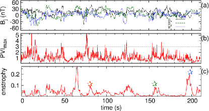
Figure 1: Sample of MMS data, plotted vs. time (seconds), beginning at 2016-01-11, 00:57:04 in the magnetosheath. (a) Magnetic field components; (b) PVI_max, calculated as the maximum of the magnetic, velocity and density intermittent time series (horizontal line represents a typical threshold); (c) Enstrophy. Stars indicate selected times at which we show ion VDFs in Fig. 2. Analyses of VDFs will refer to this time axis.

The eigenfunctions in Eq. (1) obey the orthogonality condition $\int_{-\infty}^{\infty}\psi_{m}(v)\psi_{l}(v)dv=\delta_{ml}$. Using this basis, one can obtain a 3D decomposition of the distribution function

$$f({\bm{v}})=\sum_{\bm{m}}f_{\bm{m}}\psi_{\bm{m}}({\bm{v}}),$$ (2)

where the 3D eigenfunctions are $\psi_{\bm{m}}({\bm{v}})=\psi(m_{x},v_{x})\psi(m_{y},v_{y})\psi(m_{z},v_{z})$, and the Hermite coefficients are

$$f_{\bm{m}}=\int_{-\infty}^{\infty}f({\bm{v}})\psi_{\bm{m}}({\bm{v}})d^{3}v.$$ (3)

Note that, in the case of a Maxwellian, $f(v)=M(v)=e^{-v^{2}/2}$ and the first coefficient $f_{\bm{0}}=\frac{n}{\left[2v_{th}\sqrt{\pi}\right]^{3/2}}$. This simple case gives a deep meaning to the Hermite projection in plasmas, namely that each Hermite index $m$ roughly corresponds to an order of the plasma moments: the $m=1$ coefficient corresponds to bulk flow fluctuations; $m=2$ corresponds to temperature deformations; $m=3$ to heat flux perturbations, and so on. This suggests that highly deformed VDFs would produce a distribution of modes.

MMS analysis. We now perform a Hermite analysis of the MMS data. Required projections are based on a 3D non-uniform grid in each direction based on the zeroes $v_{j}$ of the order $N_{v}+1$ Hermite polynomial, [$H_{N_{v}+1}(v_{j})=0;j=0,N_{v}+1$], thus defining a quadrature. For these results, we choose $N_{v}\equiv N_{v_{x}}=N_{v_{y}}=N_{v_{z}}=100$. This spans a velocity space, centered at zero speed, defined by values $v_{j}$ as $v_{0}=-V_{max},...,v_{N_{v}/2}=0,...,v_{N_{v}}=V_{max}$ (Zhaohua, 2014). The velocity is normalized in terms of the local thermal velocity $v_{th}$, the density is normalized such that $n=1$, and the local fluid velocity ${\bm{u}}=0$ is built into the representation as described above (velocity is measured relative to the bulk fluid frame). Values of $f({\bm{v}})$ are transformed from the native (MMS) spherical representation to the non-uniform (Cartesian) grid, using a 2^nd order interpolation method, weighting with volumes $V=\int_{v_{1}}^{v_{2}}\int_{\theta_{1}}^{\theta_{2}}\int_{\phi_{1}}^{\phi_{2}}v^{2}sin\theta~{}dvd\theta d\phi$ within each angular sector of the MMS data grid. This procedure produces a normalized VDF on a new “Hermite grid”, $f(v_{x},v_{y},v_{z})$, where velocities are in units of local thermal speed, ${\bm{u}}=0$, and unit density. The occurrence of missing data points is reduced by averaging $f({\bm{v}})$ over the four MMS satellites. When the spacecraft are closely separated, as in the present case, there are no remarkable differences among the four MMS_i datasets, and therefore this averaging does not change the following results.

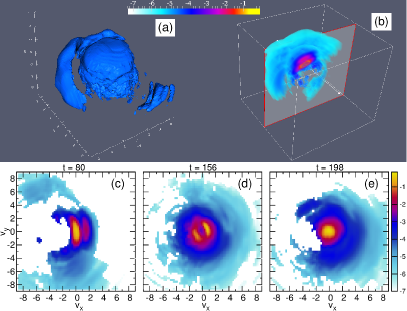
Figure 2: (a) Ion velocity distribution function, obtained from the MMS mission interpolating the function over a Hermite grid (data from $t=80$ s in Fig.1) and averaging over the 4 satellites. (b) 2D cut in the $v_{x},v_{y}$ plane, with 3D shaded contours. Panels (c), (d) and (e) represents slices of the VDF at different times, highlighted with stars in Fig. 1-(c).

Following this procedure results in a three dimensional rendering of the interpolated VDF at a single time ($t\sim 80$ s in Fig. 1), as reported in Fig. 2. The distribution is highly non-Maxwellian, as the iso-surfaces reveal the presence of secondary beams, rings of particles, multiple-anisotropies, heat flux and so on. This pictorial representation already suggests a broad spectrum of Hermite moments. The same figure shows 2D cuts of the interpolated VDF, at several different times: at $t=80$ [same as panel (a); at $t=156$; and at $t=198$ s. Fig. 1 provides the context. It is evident that there are strong non-Maxwellian deviations, with differences varying in time (and due to the high speed flow in the magnetosheath, varying in spatial position). These deformations can be initiated by different local processes (Greco et al., 2012; Howes et al., 2017).

In order to quantify deviations from fluids, we compute the mean square departure from Maxwellianity, which can also be described as the second Casimir invariant of the VDF, or, in analogy to the mean square vorticity in hydrodynamics (Knorr, 1977), an enstrophy. We define the local deviation from the associated Maxwellian $\delta f=f(v)-M(v)$, that is equivalent to subtracting $f_{0}$ from the Hermite series. Using this projection, indeed, the Parseval theorem gives the enstrophy

$$\Omega(t)\equiv\int_{-\infty}^{\infty}\delta f^{2}({\bm{v}},t)d^{3}v=\sum_{\bm{m}>0}\left[f_{\bm{m}}(t)\right]^{2}.$$ (4)

This quantity is zero for a pure Maxwellian, and may be compared with other parameters adopted as measures of non-Maxwellianity in plasma turbulence studies (Greco et al., 2012). It is also related to what is designated the “‘free energy” in certain reduced perturbative treatments of kinetic plasma (e.g., Schekochihin et al. (2008)), except that in the present case no perturbation is implied. The plasma enstrophy as a function of time is reported in Fig. 1-(c). Its behavior is quite bursty, and is qualitatively connected to the spatial intermittency of the system. For example, peaks of enstrophy frequently correspond to regions where PVI_max is high, or nearby these maxima. This is consistent with previous studies (Greco et al., 2012; Parashar and Matthaeus, 2016) that found anisotropic or non-Maxwellian features in the vicinity of magnetic coherent structures such as current sheets. The distributions shown above in Fig. 2 correspond to the times of local peaks of $\Omega(t)$ seen in Fig. 1-(c).

Following Eq. (3), we compute the modal 3D Hermite spectrum $f_{{\bm{m}}}^{2}(t)$. For an ensemble average description of the entire sample, our method averages the multidimensional Hermite spectrum over time, indicating this as $E(m_{x},m_{y},m_{z})=\langle f_{{\bm{m}}}^{2}(t)\rangle_{T}$. The 3D modal spectrum (as in Fourier analysis) permits examination of the full 3D structure of the spectral distribution. Given the great volume of data, it may be reduced or sampled to attain more compact representations. To this end, we compute the reduced 2D spectra as $E(m_{x},m_{y})=\sum_{m_{z}}E(m_{x},m_{y},m_{z})$, and analogously $E(m_{x},m_{z})$ and $E(m_{y},m_{z})$. Figure 3 shows two of these reduced spectra. Within their respective planes, these spectra are quite isotropic, indicating the absence of strong magnetization and/or other privileged directions in this stream. (Recall that plasma $\beta\sim$ 7.)

Based on the 2D spectra, a reasonable way to characterize the velocity space fluctuations for this dataset is the isotropic velocity space spectrum. The isotropic (omni-directional) Hermite spectrum, in analogy to the classical spectral density in hydrodynamic turbulence, is computed by summing $m_{x},m_{y},m_{z}$ over concentric shells of thickness $\delta$ (here, unity) in the Hermite index space. That is, $P(m)=\sum_{m-\frac{1}{2}<|{\bf m^{\prime}}|\leq m+\frac{1}{2}}E({\bf m}^{\prime})$. The isotropic Hermite spectrum of magnetosheath turbulence is reported in Fig. 3-(c). The velocity space distribution follows a power law behavior through at least the first ten moments, indicating the possibility of a phase-space turbulent cascade, as suggested in the literature (Sircombe et al., 2006; Schekochihin et al., 2008; Tatsuno et al., 2009; Schekochihin et al., 2016; Kanekar et al., 2015; Parker and Dellar, 2015).

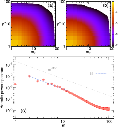
Figure 3: (a) and (b): 2D reduced Hermite spectrum, indicating spectral isotropy in these velocity space planes. (b) Power spectrum of the Hermite modes for the MMS dataset. The best fit to a power law $m^{-\alpha}$ gives $\alpha\sim 1.5$, with an error of $\sim 7\%$.

The model. The analysis suggests a cascade in the plasma moments, analogous to the classical real-space fluid cascade. To describe the inertial range of this cascade, $P(m)\sim m^{-\alpha}$, seen in Figure 3-(c) at $m<15$, we develop a turbulence theory based on qualitative arguments, in style similar to the Kolmogorov phenomenology (Kolmogorov, 1941). The Boltzmann kinetic equation for weakly-collisional plasma reads as

$$\frac{\partial f}{\partial t}+{\bm{\nabla}}\cdot{\left({\bm{v}}f\right)}+\frac{e}{M_{p}}\left({\bm{E}}+{\bm{v}}\times{\bm{B}}\right)\cdot{\bm{\nabla}}_{v}f=C_{\nu}.$$ (5)

This equation couples with the Maxwell equations to determine the electric field $\bm{E}$ and magnetic field $\bm{B}$. $M_{p}$ indicates the mass and $e$ the charge of ions. The r. h. s. of Eq. (5) is a collision operator, which may have a complex form. We make use presently of two Hermite recursion relations:

$$v~{}\psi_{m}(v)=\sqrt{\frac{m}{2}}\psi_{m-1}(v)+\sqrt{\frac{m+1}{2}}\psi_{m+1}(v),$$ (6)

$$\frac{\partial\psi_{m}(v)}{\partial v}=\sqrt{\frac{m}{2}}\psi_{m-1}(v)-\sqrt{\frac{m+1}{2}}\psi_{m+1}(v).$$ (7)

Upon computing Hermite and Fourier transforms of Eq.(5), and using Eq.s (6)-(7), one arrives at an evolution equation for the coefficients $\frac{\partial f_{\bm{m}}({\bm{k}},t)}{\partial t}$, in a 7D space (3D Fourier space, 3D Hermite space, and time). Because of the complexity of this equation, we will proceed with some ansatz, an approach familiar in Navier-Stokes turbulence. First, we neglect the collisions, which are likely to be confined to very high Hermite modes $m$’s. Second, we envision three (asymptotic) regimes, assuming locality in scale,

$$\frac{\partial f_{m}(k,t)}{\partial t}\sim\left\{\begin{aligned} &k\sqrt{m}v_{th}~{}\mathcal{S}_{m}\!\!\left\{f_{m}(k,t)\right\}&&(a),\\ &\frac{eE(k)}{M_{p}v_{th}}\sqrt{m}~{}\mathcal{D}_{m}\!\!\left\{f_{m}(k,t)\right\}&&(b),\\ &\frac{eB(k)}{M_{p}}m~{}\mathcal{A}_{m}\!\!\left\{f_{m}(k,t)\right\}&&(c).\end{aligned}\right.$$ (8)

These regimes are obtained immediately from 1D-1V models using Eq.s (6)-(7), assuming that [case (a)] the dominant term is either due to bulk and thermal fluctuations; or [case (b)], that the main fluctuations are due to the electric field; or [case (c)], that the dynamics is governed by the magnetic field. Here $E(k)$ and $B(k)$ represent the electric and magnetic spectra. In Eq. (8), $\mathcal{S}_{m}$ is a linear operator, similar to a splitting operator that propagates information into $m+1$ and $m-1$; $\mathcal{D}_{m}$ is an operator that resembles derivatives in the $m$-space (Schekochihin et al., 2016); and $\mathcal{A}_{m}$ is a higher order operator, combinations of the previous two. Note that Eq. (8)-(c) also introduces anisotropy in the $m$-space, which we will discuss in future works. In all three limits we expect redistribution of fluctuations in $m$-space, though a cascade/diffusion-like process. Following the Kolmogorov intuition, using now Eq. (8), we extract 3 characteristic times that depend on both $k$ and $m$:

$$\tau_{v}(k,m) = \frac{1}{v_{th}k\sqrt{m}}\sim m^{-1/2}$$ (9)

$$\tau_{E}(k,m) = \frac{M_{p}v_{th}}{eE(k)\sqrt{m}}\sim m^{-1/2}$$ (10)

$$\tau_{B}(k,m) = \frac{M_{p}}{eB(k)m}\sim m^{-1}.$$ (11)

These times measure in some sense the relative intensity of the corresponding terms in the dynamical system Eq. (5).

At this stage, we adopt the hypothesis of an enstrophy cascade in the velocity space. We integrate over volume, and therefore over $k$, to find a scaling law in $m$, based on the idea that a velocity cascade proceeds conserving the quadratic “rugged” invariant $\Omega$, defined in Eq.(4). The first hypothesis is that there is a net constant flux in the $m$-space, namely

$$\epsilon=\frac{f_{m}^{2}}{\tau_{m}}=const.$$ (12)

where $\tau_{m}$ is the spectral transfer time for the enstrophy. The second hypothesis concerns choice of the characteristic time of this cascade, the simplest options being to chose among (9)-(11). Third (and last), from simple dimensional arguments,

$$\Omega=\langle\int\delta f^{2}d^{3}v\rangle_{x}=\sum_{m>0}f_{m}^{2}=\int P(m)dm,$$

$$\rightarrow P(m)\sim f_{m}^{2}m^{-1},$$ (13)

where we defined $\langle...\rangle_{x}$ as the physical space volume average. Using Eq.s (12), (13) and a characteristic time such as (9) or (10), one gets

$$P(m)\sim m^{-3/2}.$$ (14)

Analogously, using Eq.s (12) and (13), coupled with (11) one obtains

$$P(m)\sim m^{-2}.$$ (15)

The first law in Eq. (14) should be valid in a thermal and/or electric-dominated regime, while the last prediction is more adequate for a highly magnetized (anisotropic) plasma. For the present observation, we fit an inertial range powerlaw to the velocity-space cascade, as shown in Figure 3-(c), obtaining $P(m)\sim m^{-\alpha}$, with $\alpha=1.5\pm 0.1$, in agreement with Eq. (14).

To summarize and conclude, we have carried out an analysis of MMS ion VDF data to visualize and describe the ion distribution function in this low-collisonality space plasma with unprecedented temporal and velocity-scale resolution. We observe here in spacecraft data the same kind of fine scale velocity structure reported frequently in Vlasov simulations Servidio et al. (2015); Howes et al. (2017). This motivates a further analysis of the velocity space structure in terms of a Hermite spectral analysis, which has the physically interesting heuristic interpretation as a moment heirarchy. The power law that emerges in moments (Hermite indices) suggests a velocity space cascade. We pursue this in a very preliminary way, in analogy to classical hydrodynamics cascade. One first identifies a conserved flux across scale – here the velocity space enstrophy (or, free energy) – and the associated dynamical time scales. From this emerges the possibility of spectral slopes between -2 and -3/2. Other possibilities may exist for other physical regimes in which different time scales become available. For the MMS magnetosheath interval analyzed here, the -3/2 slope seems to be clearly favored, suggesting that the velocity space cascade for this interval is governed by thermal and/or electric effects (Valentini and Veltri, 2009).

This observation and analysis is preliminary, being based on a single set of high resolution observations, and so we must eschew any assignment of universality. However, enabled by significant advances in diagnostics such as those offered by MMS, this approach to understanding velocity space structure may prove to be fruitful for further studies in turbulent plasmas, in varying conditions.