New numerical approach for fractional differential equations

Abstract

In the present case, we propose the correct version of the fractional Adams-Bashforth methods which take into account the nonlinearity of the kernels including the power law for the Riemann-Liouville type, the exponential decay law for the Caputo-Fabrizio case and the Mittag-Leffler law for the Atangana-Baleanu scenario.The Adams-Bashforth method for fractional differentiation suggested and are commonly use in the literature nowadays is not mathematically correct and the method was derived without taking into account the nonlinearity of the power law kernel. Unlike the proposed version found in the literature, our approximation, in all the cases, we are able to recover the standard case whenever the fractional power $\alpha=1$.

2010 Mathematics Subject Classification: 26A33, 34A34, 65M06

Keywords: Caputo derivative; Fractional differential equation.

1 Introduction

Fractional calculus is known to be a generalization of the standard or integer-order calculus with a history of not less than over three centuries. It can be dated back to Leibniz’s letter to L’Hospital, in which the meaning of the one-half order derivative was first introduced and discussed [14]. Although fractional calculus has such a long history, most of the research conducted still stay in the realm of theory, due to the lack of proper mathematical analysis methods and real applications.

Until the past decades, when many researchers pointed out that fractional derivative and fractional differential equation do have many applications in various fields. Differential problems with fractional derivative order have now become the most useful and powerful tools for describing nonlinear phenomena that are encountered in many application areas of biology, chemistry, ecology, engineering and various domains of applied sciences. A lot of mathematical models, such as in viscoelastic mechanics, acoustic dissipation, boundary layer effects in duct, biomedical engineering, power-law phenomena in fluid and complex network, allometric scaling laws in mathematical ecology and epidemiology, control theory, continuous time random walk, dielectric polarization, porous media, quantitative finance, quantum evolution of complex systems, Lévy statistics, fractional Brownian, fractional signal and image processing, electrode-electrolyte polarization, electromagnetic waves, filters motion, phase-locked loops and non-local phenomena have justified to give a better description of the phenomenon under investigation than models with the integer order derivative [1, 10].

Nowadays, there have been a lot studies on approximate methods for fractional differential equations. For instance, Dithelm et al. and Li et al., have reported some results on numerical fractional ordinary differential equations [7, 12]. When seeking an approximate solution to the fractional order ordinary and partial differential equations, among many other choices that have been used are include the Adomian decomposition, homotopy perturbation and differential transform methods, for example, see [11, 15]. A lot has been reported in the literature on various fractional derivatives, ranging from the Riemann-Liouville to Atangana-Baleanu fractional derivative versions [5, 6, 3]. Not only that, when numerically simulating such models, different numerical approximation techniques have been adopted in both space [16, 17, 18, 19, 20, 21] and time [4, 8, 9].

The Adams-Bashforth has been recognized as a great and powerful numerical method able to provide a numerical solution closer to the exact solution. This method was developed with the classical differentiation using the fundamental theorem of calculus and taking the difference between two times including $t_{n+1}$ and $t_{n}$. This method was later extended to the concept of fractional differentiation with Caputo and Riemann-Liouville derivatives, however, the adaptation was not mathematically correct as the kernel of fractional integration is non-linear. In addition to this when the fractional order $\alpha=1$ with this fractional version, we do not recover the classical Adams-Bashforth numerical scheme. In this paper, we will propose a new Adams-Bashforth for fractional differentiation with Caputo, Caputo-Fabrizio and Atangana-Baleanu derivatives, this version takes into account the nonlinearity of the kernels including the power law for Riemann-Liouville case, the exponential decay law for Caputo-Fabrizio case and Mittag-Leffler for Atangana-Baleanu case. Indeed when the fractional order turns to 1 one is expected to recover the classical Adams-Bashforth method.

2 Preliminaries

In this section, we recall some basic definitions and properties of fractional calculus theory which are useful in the next sections.

Definition 2.1.

The Caputo fractional derivative of order $\alpha>0$ is defined by

$${}_{0}^{C}\mathsf{D}_{t}^{\alpha}y(t)=\frac{1}{\Gamma(\alpha)}\int_{0}^{t}f(\lambda,y(\lambda))(t-\lambda)^{\alpha-1}d\lambda$$ (2.1)

Definition 2.2.

Let $y\in H^{1}(a,b),\;b>a$ and $\alpha\in[0,1]$. Then the new Caputo version of fractional derivative is defined as

$${}_{0}^{CF}\mathsf{D}_{t}^{\alpha}y(t)=\frac{M(\alpha)}{1-\alpha}\int_{a}^{t}y^{\prime}(\tau)\exp\left[-\frac{\alpha}{1-\alpha}(t-\tau)\right]d\tau$$ (2.2)

where $M(\alpha)$ is a normalization function, such that $M(0)=M(1)=1$ [2, 5, 6, 13]. Nevertheless, if the function $y\notin H^{1}[a,b]$ then, the new derivative called the Caputo-Fabrizio fractional derivative can be defined as

$${}_{0}^{CF}\mathsf{D}_{t}^{\alpha}y(t)=\frac{M(\alpha)}{1-\alpha}\int_{0}^{t}y^{\prime}(\tau)\exp\left[-\frac{\alpha}{1-\alpha}(t-\tau)\right]d\tau.$$ (2.3)

Theorem 2.3.

Let $y(t)$ be a function for which the Caputo-Fabrizio exists, then, the Sumudu transform of the Caputo-Fabrizio fractional derivative of $y(t)$ is given as

$$ST\left({}^{CF}_{0}\mathcal{D}_{t}^{\alpha}\right)(y(t))=M(\alpha)\frac{SF(y(t))-y(0)}{1-\alpha+\alpha u}$$ (2.4)

Proof.

See Atangana [1] for detail. ∎

Atangana and Baleanu [3] proposed the following derivatives.

Definition 2.4.

Let $y\in H^{1}(a,b),\;a<b,\;\;\alpha\in[0,1]$ then, the definition of the Atangana and Baleanu fractional derivative in Caputo sense is given as [3]

$$^{ABC}_{a}\mathcal{D}_{t}^{\alpha}[y(t)]=\frac{M(\alpha)}{1-\alpha}\int_{a}^{t}y^{\prime}(\tau)E_{\alpha}\left[-\alpha\frac{(t-\tau)^{\alpha}}{1-\alpha}\right]d\tau$$ (2.5)

where $M(\alpha)$ has the same properties as in the case of the Caputo-Fabrizio fractional derivative.

The above definition is considered to be useful to discuss real world problems, and it will also be a great advantage when applying the Laplace transform to solve some real life (physical) models with initial conditions. However, it should be noted that we do not recover the original function when $\alpha=0$ except when at the origin the function vanishes. To avoid this kind of problem, the following definition is proposed.

Definition 2.5.

Let $y\in H^{1}(a,b),\;a<b,\;\;\alpha\in[0,1]$ then, the definition of the Atangana-Baleanu fractional derivative in Riemann-Liouville sense becomes [3]

$$^{ABR}_{a}\mathcal{D}_{t}^{\alpha}[y(t)]=\frac{M(\alpha)}{1-\alpha}\frac{d}{dt}\int_{a}^{t}y(\tau)E_{\alpha}\left[-\alpha\frac{(t-\tau)^{\alpha}}{1-\alpha}\right]d\tau$$ (2.6)

clearly, both equations (2.5) and (2.6) have a non-local kernel. We also obtain zero whenever the function in equation (2.5) is constant.

3 Numerical techniques for fractional differential equations

The aim of this section is to introduce a new numerical approximation approach based on the Caputo, Caputo-Fabrizio and Atangana-Baleanu fractional derivatives for the discretization of fractional differential equations. We also give the stability and convergence results for each of the derivatives.

3.1 The Caputo fractional derivative

We consider the following fractional differential equation

$$_{0}^{C}\mathsf{D}_{t}^{\alpha}y(t)=f(t,y(t))$$ (3.7)

By applying the fundamental theorem of calculus on equation (3.7), we obtain

$$y(t)-y(0)=\frac{1}{\Gamma(\alpha)}\int_{0}^{t}f(\lambda,y(\lambda))(t-\lambda)^{\alpha-1}d\lambda,$$ (3.8)

thus at $t=t_{n+1},\;n=0,1,2,\ldots$, we obtain

$$y(t_{n+1})-y(0)=\frac{1}{\Gamma(\alpha)}\int_{0}^{t_{n+1}}(t_{n+1}-t)^{\alpha-1}f(t,y(t))dt$$ (3.9)

and

$$y(t_{n})-y(0)=\frac{1}{\Gamma(\alpha)}\int_{0}^{t_{n}}(t_{n}-t)^{\alpha-1}f(t,y(t))dt$$ (3.10)

By subtracting (3.10) from (3.9), we get

$$y(t_{n+1})=y(t_{n})+\frac{1}{\Gamma(\alpha)}\int_{0}^{t_{n+1}}(t_{n+1}-t)^{\alpha-1}f(t,y(t))dt+\frac{1}{\Gamma(\alpha)}\int_{0}^{t_{n}}(t_{n}-t)^{\alpha-1}f(t,y(t))dt.$$

This implies that

$$y(t_{n+1})=y(t_{n})+A_{\alpha,1}+A_{\alpha,2}$$ (3.11)

where

$$A_{\alpha,1}=\frac{1}{\Gamma(\alpha)}\int_{0}^{t_{n+1}}(t_{n+1}-t)^{\alpha-1}f(t,y(t))dt$$

and

$$A_{\alpha,2}=\frac{1}{\Gamma(\alpha)}\int_{0}^{t_{n}}(t_{n}-t)^{\alpha-1}f(t,y(t))dt,$$

the function $f(t,y(t))$ can be approximated using the Lagrange interpolation as

$$P(t)\simeq\frac{t-t_{n-1}}{t_{n}-t_{n-1}}f(t_{n},y_{n})+\frac{t-t_{n}}{t_{n-1}-t_{n}}f(t_{n-1},y_{n-1})$$

$$=\frac{f(t_{n},y_{n})}{h}(t-t_{n-1})-\frac{f(t_{n-1},y_{n-1})}{h}(t-t_{n}).$$ (3.12)

Thus,

$$A_{\alpha,1}=\frac{f(t_{n},y_{n})}{h\Gamma(\alpha)}\int_{0}^{t_{n+1}}(t_{n+1}-t)^{\alpha-1}(t-t_{n-1})dt-\frac{f(t_{n-1},y_{n-1})}{\Gamma(\alpha)h}\int_{0}^{t_{n+1}}(t_{n+1}-t)(t-t_{n})dt$$ (3.13)

$$A_{\alpha,1} = \frac{f(t_{n},y_{n})}{h\Gamma(\alpha)}\int_{0}^{t_{n+1}}y^{\alpha-1}(t_{n+1-y-t_{n-1}})dy-\frac{f(t_{n-1},y_{n-1})}{\Gamma(\alpha)h}\int_{0}^{t_{n+1}}y^{\alpha-1}(t_{n+1}-y-t_{n})dy$$ (3.14)

$$= \frac{f(t_{n},y_{n})}{h\Gamma(\alpha)}\left\{\frac{2ht^{\alpha}_{n+1}}{\alpha}-\frac{t^{\alpha+1}_{n+1}}{\alpha+1}\right\}-\frac{f(t_{n-1},y_{n-1})}{h\Gamma(\alpha)}\left\{\frac{ht^{\alpha}_{n+1}}{\alpha}-\frac{t^{\alpha+1}_{n+1}}{\alpha+1}\right\}$$

Therefore,

$$A_{\alpha,1}=\frac{f(t_{n},y_{n})}{h\Gamma(\alpha)}\left\{\frac{2h}{\alpha}t_{n+1}^{\alpha}-\frac{t_{n+1}^{\alpha+1}}{\alpha+1}\right\}-\frac{f(t_{n-1},y_{n-1})}{h\Gamma(\alpha)}\left\{\frac{h}{\alpha}t_{n+1}^{\alpha}-\frac{t_{n+1}^{\alpha+1}}{\alpha+1}\right\}.$$ (3.15)

Similarly, we obtain

$$A_{\alpha,2} = \frac{f(t_{n},y_{n})}{h\Gamma(\alpha)}\int_{0}^{t_{n}}(t_{n}-t)^{\alpha-1}(t-t_{n-1})dt-\frac{(t_{n-1},y_{n-1})}{h\Gamma(\alpha)}\int_{0}^{t_{n}}(t_{n}-t)^{\alpha-1}(t-t_{n})dt$$

$$= \frac{f(t_{n},y_{n})}{h\Gamma(\alpha)}\int_{0}^{t_{n}}y^{\alpha-1}\left\{t_{n}-y-t_{n-1}\right\}dy+\frac{f(t_{n-1},y_{n-1})}{h\Gamma(\alpha)}\frac{t^{\alpha+1}_{n}}{\alpha}$$

$$= \frac{f(t_{n},y_{n})}{h\Gamma(\alpha)}\left\{\frac{ht^{\alpha}_{n}}{\alpha}-\frac{t^{\alpha+1}_{n}}{\alpha+1}\right\}+\frac{f(t_{n-1},y_{n-1})}{h\Gamma(\alpha+1)}t_{n}^{\alpha+1}.$$

Thus the approximate solution is given as

$$y(t_{n+1}) = y(t_{n})+\frac{f(t_{n},y_{n})}{h\Gamma(\alpha)}\left\{\frac{2h}{\alpha}t^{\alpha}_{n+1}-\frac{t_{n+1}^{\alpha+1}}{\alpha+1}+\frac{h}{\alpha}t_{n}^{\alpha}-\frac{t_{n}^{\alpha+1}}{\alpha}\right\}$$ (3.17)

$$+\frac{f(t_{n-1},y_{n-1})}{h\Gamma(\alpha)}\left\{\frac{h}{\alpha}t^{\alpha}_{n+1}-\frac{t_{n+1}^{\alpha+1}}{\alpha+1}+\frac{t_{n}^{\alpha}}{\alpha+1}\right\}.$$

Theorem 3.1.

Let

$${}_{0}^{C}\mathsf{D}_{t}^{\alpha}y(t)=f(t,y(t))$$

be a fractional differential equation such that $f$ is bounded, then the numerical solution of $y(t)$ is given by

$$y(t_{n+1}) = y(t_{n})+\frac{f(t_{n},y_{n})}{h\Gamma(\alpha)}\left\{\frac{2h}{\alpha}t^{\alpha}_{n+1}-\frac{t_{n+1}^{\alpha+1}}{\alpha+1}+\frac{h}{\alpha}t_{n}^{\alpha}-\frac{t_{n}^{\alpha+1}}{\alpha}\right\}$$

$$+\frac{f(t_{n-1},y_{n-1})}{h\Gamma(\alpha)}\left\{\frac{h}{\alpha}t^{\alpha}_{n+1}-\frac{t_{n+1}^{\alpha+1}}{\alpha+1}+\frac{t_{n}^{\alpha}}{\alpha+1}\right\}+R_{n}^{\alpha}(t)$$

where

$$R_{n}^{\alpha}(t)<\frac{h^{3+\alpha}M}{12\Gamma(\alpha+1)}\left\{(n+1)^{\alpha}+n^{2}\right\}$$

Proof.

Following the derivation presented earlier, we have

$$y(t_{n+1})=y(t_{n})+\frac{1}{\Gamma(\alpha)}\int_{0}^{t_{n+1}}(t_{n+1}-t)^{\alpha-1}f(t,y(t))dt-\frac{1}{\Gamma(\alpha)}\int_{0}^{t_{n}}(t_{n+1}-t)^{\alpha-1}f(t,y(t))dt.$$

Using the Lagrange polynomial, we have

$$y(t_{n+1})-y(t_{n}) = \frac{1}{\Gamma(\alpha)}\int_{0}^{t_{n+1}}L_{1}(t)(t_{n+1}-t)^{\alpha-1}dt+\frac{1}{\Gamma(\alpha)}\int_{0}^{t_{n+1}}R_{1}(t)(t_{n+1}-t)^{\alpha-1}dt$$ (3.18)

$$-\frac{1}{\Gamma(\alpha)}\int_{0}^{t_{n}}L_{2}(t)(t_{n}-t)^{\alpha-1}dt+\frac{1}{\Gamma(\alpha)}\int_{0}^{t_{n}}R_{2}(t)(t_{n}-t)^{\alpha-1}dt$$

$$= \frac{f(t_{n},y_{n})}{h\Gamma(\alpha)}\left\{\frac{2h}{\alpha}t^{\alpha}_{n+1}-\frac{t_{n+1}^{\alpha+1}}{\alpha+1}+\frac{ht^{\alpha}}{\alpha}-\frac{t^{\alpha+1}}{\alpha+1}\right\}+\frac{f(t_{n-1},y_{n-1})}{h\Gamma(\alpha)}$$

$$\times\left\{\frac{ht_{n+1}^{\alpha}}{\alpha}-\frac{t_{n+1}^{\alpha+1}}{\alpha+1}+\frac{t_{n}^{\alpha}}{\alpha+1}\right\}+\frac{1}{\Gamma(\alpha)}\int_{0}^{t_{n+1}}R(t)(t_{n+1}-t)^{\alpha-1}dt$$

$$-\frac{1}{\Gamma(\alpha)}\int_{0}^{t_{n}}R(t)(t_{n}-t)^{\alpha-1}dt.$$

Next, we let

$$R_{n}(t)=\frac{1}{\Gamma(\alpha)}\int_{0}^{t_{n+1}}R_{1}(t)(t_{n+1}-t)^{\alpha-1}dt-\frac{1}{\Gamma(\alpha)}\int_{0}^{t_{n}}R_{1}(t)(t_{n}-t)^{\alpha-1}dt$$

where

$$R_{1}(t)=\frac{f^{(n+1)}(t,y(t))}{(n+1)!}\prod_{i=0}^{n}(t-t_{i})$$

$$R_{n}(t) = \frac{1}{\Gamma(\alpha)}\int_{0}^{t_{n+1}}\frac{f^{(n+1)}(t,y(t))}{(n+1)!}\prod_{i=0}^{n}(t-t_{i})(t_{n+1}-t)^{\alpha-1}dt$$

$$-\frac{1}{\Gamma(\alpha)}\int_{0}^{t_{n}}\frac{f^{(n+1)}(t,y(t))}{(n+1)!}\prod_{i=0}^{n}(t-t_{i})(t_{n}-t)^{\alpha-1}dt.$$

Let $\|f(t)\|_{\infty}=\sup_{t\in[a,b]}|f(t)|$, we assume that

$$\|f^{(3)}(t,y(t))\|_{\infty}<M<\infty$$

then

$$\|R_{n}(t)\|_{\infty} = \left\|\frac{1}{\Gamma(\alpha)}\int_{0}^{t_{n+1}}\frac{f^{(3)}(t,y(t))}{(n+1)!}\prod_{i=0}^{n}(t-t_{i})(t_{n+1}-t)^{\alpha-1}dt\right.$$

$$\left.-\frac{1}{\Gamma(\alpha)}\int_{0}^{t_{n}}\frac{f^{(n+1)}(t,y(t))}{(n+1)!}\prod_{i=0}^{n}(t-t_{i})(t_{n}-t)^{\alpha-1}dt\right\|_{\infty}$$

$$\|R_{n}(t)\|_{\infty} \leq \left\|\frac{1}{\Gamma(\alpha)}\int_{0}^{t_{n+1}}\frac{f^{(n+1)}(t,y(t))}{(n+1)!}\prod_{i=0}^{n}(t-t_{i})(t_{n+1}-t)^{\alpha-1}dt\right.$$

$$\left.-\frac{1}{\Gamma(\alpha)}\int_{0}^{t_{n}}\frac{f^{(n+1)}(t,y(t))}{(n+1)!}\prod_{i=0}^{n}(t-t_{i})(t_{n}-t)^{\alpha-1}dt\right\|_{\infty}.$$

Without loss of generality, we evaluate

$$\left\|\frac{1}{6\Gamma(\alpha)}\int_{0}^{t_{n+1}}f^{(3)}(t,y(t))\prod_{i=0}^{2}(t-t_{i})(t_{n}-t)^{\alpha-1}dt\right\|_{\infty}$$

$$\hskip 56.9055pt\leq\frac{1}{6\Gamma(\alpha)}\int_{0}^{t_{n+1}}\left\|f^{(3)}(t,y(t))\right\|_{\infty}\left\|\prod_{i=0}^{2}(t-t_{i})\right\|(t_{n+1}-t)^{\alpha-1}dt$$

$$\hskip 56.9055pt\leq\frac{1}{6\Gamma(\alpha)}\left\|f^{(3)}(t,y(t))\right\|_{\infty}\left\|\prod_{i=0}^{2}(t-t_{i})\right\|\int_{0}^{t_{n+1}}(t_{n+1}-t)^{\alpha-1}dt$$

$$\hskip 56.9055pt\leq\frac{2h^{3}}{4\times 6\Gamma(\alpha)}\left\|f^{(3)}(t,y(t))\right\|_{\infty}\frac{t_{n+1}^{\alpha}}{\alpha}$$

$$\hskip 56.9055pt<\frac{h^{3}t_{n+1}^{\alpha}M}{12\Gamma(\alpha+1)},$$

therefore,

$$\left\|\frac{1}{\Gamma(\alpha)}\int_{0}^{t_{n+1}}\frac{f^{(n+1)}(t,y(t))}{(n+1)!}\prod_{i=0}^{n}(t-t_{i})(t_{n+1}-t)^{\alpha-1}dt\right\|_{\infty}<\frac{h^{3}t_{n+1}^{\alpha}M}{12\Gamma(\alpha+1)}$$

and

$$\left\|\frac{1}{\Gamma(\alpha)}\int_{0}^{t_{n}}\frac{f^{(n+1)}(t,y(t))}{(n+1)!}\prod_{i=0}^{n}(t-t_{i})(t_{n}-t)^{\alpha-1}dt\right\|_{\infty}<\frac{h^{3}t_{n}^{\alpha}M}{12\Gamma(\alpha+1)}$$

thus

$$\|R(t)\|_{\infty} < \frac{h^{3}M}{12\Gamma(\alpha+1)}(t^{\alpha}_{n+1}+t^{\alpha}_{n})$$

$$< \frac{h^{3+\alpha}M}{12\Gamma(\alpha+1)}\left((n+1)^{\alpha}+n^{\alpha}\right)$$

Again, we evaluate

$$\|y_{n+1}-y_{n}\|_{\infty} = \left\|\frac{1}{\Gamma(\alpha)}\int_{0}^{t_{n+1}}(t_{n+1}-t)^{\alpha-1}f(t,y(t))dt\right.$$

$$\left.-\frac{1}{\Gamma(\alpha)}\int_{0}^{t_{n}}(t_{n}-t)^{\alpha-1}f(t,y(t))dt\right\|_{\infty}$$

$$\leq \left\|\frac{1}{\Gamma(\alpha)}\int_{0}^{t_{n+1}}(t_{n+1}-t)^{\alpha-1}f(t,y(t))dt\right\|_{\infty}+$$

$$\left\|\frac{1}{\Gamma(\alpha)}\int_{0}^{t_{n}}(t_{n}-t)^{\alpha-1}f(t,y(t))dt\right\|_{\infty}.$$

Without loss of generality, we focus on

$$\left\|\frac{1}{\Gamma(\alpha)}\int_{0}^{t_{n+1}}(t_{n+1}-t)^{\alpha-1}f(t,y(t))dt\right\|_{\infty}$$

$$\hskip 56.9055pt\leq\left\|\frac{1}{\Gamma(\alpha)}\sum_{j=0}^{n}\int_{t_{j}}^{t_{j+1}}(t_{n+1}-t)^{\alpha-1}f(t_{j},y(t_{j}))dt\right\|_{\infty}$$

$$\hskip 56.9055pt\leq\frac{1}{\Gamma(\alpha)}\sum_{j=0}^{n}\int_{t_{j}}^{t_{j+1}}(t_{n+1}-t)^{\alpha-1}\left\|f(t_{j},y(t_{j}))dt\right\|_{\infty}$$

$$\hskip 56.9055pt\leq\frac{1}{\Gamma(\alpha)}\max_{t\in[t_{j},t_{j+1}]}\|f(t_{j},y(t_{j}))\|\sum_{j=0}^{n}\int_{t_{j}}^{t_{j+1}}(t_{n+1}-t)^{\alpha-1}dt$$

$$\hskip 56.9055pt\leq\frac{1}{\Gamma(\alpha)}\max_{t\in[t_{j},t_{j+1}]}\|f(t_{j},y(t_{j}))\|\sum_{j=0}^{n}\left\{\frac{(t_{n+1}-t_{j})^{\alpha}}{\alpha}-\frac{(t_{n+1}-t_{j+1})^{\alpha}}{\alpha}\right\}$$

$$\hskip 56.9055pt\leq\frac{h^{\alpha}}{\Gamma(\alpha+1)}\max_{t\in[t_{j},t_{j+1}]}\|f(t_{j},y(t_{j}))\|\sum_{j=0}^{n}\left\{(n+1-j)^{\alpha}-(n-j)^{\alpha}\right\}$$

$$\hskip 56.9055pt\leq\frac{h^{\alpha}}{\Gamma(\alpha+1)}\max_{t\in[t_{j},t_{j+1}]}\|f(t_{j},y(t_{j}))\|\left\{(n+1)^{\alpha}+1\right\}$$

$$\hskip 56.9055pt\leq\frac{h^{\alpha}}{\Gamma(\alpha+1)}\max_{t\in[t_{j},t_{j+1}]}\|f(t,y(t))\|\left\{(n+1)^{\alpha}+1\right\}$$

Thus

$$\|\frac{1}{\Gamma(\alpha)}\int_{0}^{t_{n+1}}(t_{n+1}-t)^{\alpha-1}f(t,y(t))\|<\frac{h^{\alpha}C_{n}^{\alpha}}{\Gamma(\alpha+1)}\max_{t\in[t_{j},t_{j+1}]}\|f(t,y(t))\|$$

and

$$\|\frac{1}{\Gamma(\alpha)}\int_{0}^{t_{n}}(t_{n}-t)^{\alpha-1}f(t,y(t))\|<\frac{h^{\alpha}S_{n}^{\alpha}}{\Gamma(\alpha+1)}\max_{t\in[t_{j},t_{j+1}]}\|f(t,y(t))\|$$

Therefore

$$\|y_{n+1}-y_{n}\|_{\infty}<\frac{h^{\alpha}}{\Gamma(\alpha+1)}\max_{t\in[t_{j},t_{j+1}]}\|f(t,y(t))\|\left\{C_{n}^{\alpha}+S_{n}^{\alpha}\right\}.$$

The proof is completed. ∎

3.2 The Caputo-Fabrizio fractional derivative

We next consider the following general fractional differential equation with fading memory included via the Caputo-Fabrizio fractional derivative. That is,

$$_{0}^{CF}\mathsf{D}_{t}^{\alpha}y(t)=f(t,y(t))$$ (3.19)

or

$$\frac{M(\alpha)}{1-\alpha}\int_{0}^{t}y^{\prime}(\tau)\exp\left[-\frac{\alpha}{1-\alpha}(t-\tau)\right]d\tau=f(t,y(t)).$$ (3.20)

Using the fundamental theorem of calculus, we convert the above to

$$y(t)-y(0)=\frac{1-\alpha}{M(\alpha)}f(t,y(t))+\frac{\alpha}{M(\alpha)}\int_{0}^{t}f(\tau,y(\tau))d\tau$$ (3.21)

so that

$$y(t_{n+1})-y(0)=\frac{1-\alpha}{M(\alpha)}f(t_{n},y(t_{n}))+\frac{\alpha}{M(\alpha)}\int_{0}^{t_{n+1}}f(t,y(t))dt$$ (3.22)

and

$$y(t_{n})-y(0)=\frac{1-\alpha}{M(\alpha)}f(t_{n-1},y(t_{n-1}))+\frac{\alpha}{M(\alpha)}\int_{0}^{t_{n}}f(t,y(t))dt$$ (3.23)

On removing (3.23) from (3.22) we obtain

$$y(t_{n+1})-y(t_{n})=\frac{1-\alpha}{M(\alpha)}\left\{f(t_{n},y_{n})-f(t_{n-1},y_{n-1})\right\}+\frac{\alpha}{M(\alpha)}\int_{t_{n}}^{t_{n+1}}f(t,y(t))dt$$ (3.24)

where

$$\int_{t_{n}}^{t_{n+1}}f(t,y(t))dt = \int_{t_{n}}^{t_{n+1}}\left\{\frac{f(t_{n},y_{n})}{h}(t-t_{n-1})-\frac{f(t_{n-1},y_{n-1})}{h}(t-t_{n})\right\}dt$$ (3.25)

$$= \frac{3h}{2}{f(t_{n},y_{n})}-\frac{h}{2}f(t_{n-1},y_{n-1}).$$

Thus,

$$y(t_{n+1})-y(t_{n}) = \frac{1-\alpha}{M(\alpha)}=\left[f(t_{n},y_{n})-f(t_{n-1},y_{n-1})\right]+\frac{3\alpha h}{2M(\alpha)}{f(t_{n},y_{n})}$$

$$-\frac{\alpha h}{2M(\alpha)}f(t_{n-1},y_{n-1})$$

which implies that

$$y(t_{n+1})-y(t_{n})=\left(\frac{1-\alpha}{M(\alpha)}+\frac{3\alpha h}{2M(\alpha)}\right)f(t_{n},y_{n})+\left(\frac{1-\alpha}{M(\alpha)}+\frac{\alpha h}{2M(\alpha)}\right)f(t_{n-1},y_{n-1}).$$

Hence,

$$y_{n+1}=y_{n}+\left(\frac{1-\alpha}{M(\alpha)}+\frac{3\alpha h}{2M(\alpha)}\right)f(t_{n},y_{n})+\left(\frac{1-\alpha}{M(\alpha)}+\frac{\alpha h}{2M(\alpha)}\right)f(t_{n-1},y_{n-1})$$ (3.26)

which is the corresponding two-step Adams-Bashforth method for the Caputo-Fabrizio fractional derivative. The following theorems present the convergence and stability results.

Theorem 3.2.

Let $y(t)$ be a solution of ${}_{0}^{CF}\mathsf{D}_{t}^{\alpha}y(t)=f(t,y(t))$ where $f$ is a continuous function bounded for the Caputo-Fabrizio fractional derivative, we have

$$y_{n+1}=y_{n}+\left(\frac{1-\alpha}{M(\alpha)}+\frac{3\alpha h}{2M(\alpha)}\right)f(t_{n},y_{n})+\left(\frac{1-\alpha}{M(\alpha)}+\frac{\alpha h}{2M(\alpha)}\right)f(t_{n-1},y_{n-1})+R^{n}_{\alpha}$$

where $\|R^{n}_{\alpha}\|\leq M$.

Proof.

According to the definition of the Caputo-Fabrizio derivative, we have

$$y(t)-y(0)=\frac{1-\alpha}{M(\alpha)}f(t,y(t))+\frac{\alpha}{M(\alpha)}\int_{0}^{t}f(\tau,y(\tau))d\tau.$$ (3.27)

At point $t_{n+1}$, we get

$$y(t_{n+1})=\frac{1-\alpha}{M(\alpha)}f(t_{n},y(t_{n}))+\frac{\alpha}{M(\alpha)}\int_{0}^{t_{n+1}}f(t,y(t))dt,$$

also, at point $t_{n}$ we have

$$y(t_{n})=\frac{1-\alpha}{M(\alpha)}f(t_{n-1},y(t_{n-1}))+\frac{\alpha}{M(\alpha)}\int_{0}^{t_{n}}f(t,y(t))dt.$$

Thus,

$$y(t_{n+1})-y(t_{n}) = \frac{1-\alpha}{M(\alpha)}\left\{f(t_{n},y_{n})-f(t_{n-1},y(t_{n-1}))\right\}+\frac{\alpha}{M(\alpha)}\int_{t_{n}}^{t_{n+1}}f(t,y(t))dt$$ (3.28)

$$= \frac{1-\alpha}{M(\alpha)}\left\{f(t_{n},y_{n})-f(t_{n-1},y(t_{n-1}))\right\}+\frac{\alpha}{M(\alpha)}\left\{\frac{f(t_{n},y_{n})}{h}(t-t_{n-1})\right.$$

$$\left.-\frac{f(t_{n-1},y_{n-1})}{h}(t-t_{n})+\sum_{i=2}^{n}\prod_{i=2}^{n}\frac{(t-t_{i})}{h(-1)^{i}}f(t_{i},y_{i})\right\}dt$$

so that

$$y_{n+1} = y_{n}+\left(\frac{1-\alpha}{M(\alpha)}+\frac{3\alpha h}{2M(\alpha)}\right)f(t_{n},y_{n})+\left(\frac{1-\alpha}{M(\alpha)}+\frac{\alpha h}{M(\alpha)}\right)f(t_{n-1},y_{n-1})$$ (3.29)

$$+\underbrace{\frac{\alpha}{M(\alpha)}\int_{t_{n}}^{t_{n+1}}\sum_{i=2}^{n}\prod_{i=2}^{n}\frac{(t-t_{i})}{h(-1)^{i}}f(t_{i},y_{i})dt}_{\text{error term}}$$

We denote the above error term by

$$R_{\alpha}^{n}=\frac{\alpha}{M(\alpha)}\int_{t_{n}}^{t_{n+1}}\sum_{i=2}^{n}\prod_{i=2}^{n}\frac{(t-t_{i})}{h(-1)^{i}}f(t_{i},y_{i})dt$$

Thus

$$\left\|R_{\alpha}^{n}\right\|_{\infty} = \frac{\alpha}{M(\alpha)}\left\|\int_{t_{n}}^{t_{n+1}}\sum_{i=2}^{n}\prod_{i=2}^{n}\frac{(t-t_{i})}{h(-1)^{i}}f(t_{i},y_{i})dt\right\|_{\infty}$$ (3.30)

$$\leq \frac{\alpha}{M(\alpha)}\int_{t_{n}}^{t_{n+1}}\left\|\sum_{i=2}^{n}\prod_{i=2}^{n}\frac{(t-t_{i})}{h(-1)^{i}}f(t_{i},y_{i})dt\right\|_{\infty}$$

$$\leq \frac{\alpha}{M(\alpha)}\int_{t_{n}}^{t_{n+1}}\sum_{i=2}^{n}\prod_{i=2}^{n}\left|\frac{(t-t_{i})}{h(-1)^{i}}\right|\left\|f(t_{i},y_{i})dt\right\|_{\infty}$$

$$< \frac{\alpha}{M(\alpha)}\int_{t_{n}}^{t_{n+1}}\sum_{i=2}^{n}\prod_{i=2}^{n}\frac{\left|(t-t_{i})\right|}{h}\sup_{i\in I}\left\{\max_{i\in I}|f(t_{i},y_{i})|\right\}$$

$$< \frac{\alpha}{M(\alpha)}\frac{(n+1)!h^{n+1}}{4}M.$$

Hence,

$$\left\|R_{\alpha}^{n}\right\|_{\infty}<\frac{\alpha}{M(\alpha)}(n+1)!h^{n+1}M.$$

∎

Theorem 3.3.

Let $y(t)$ be a solution of ${}_{0}^{CF}\mathsf{D}_{t}^{\alpha}y(t)=f(t,y(t))$, for every $n\in N$

$$\|y_{n+1}-y_{n}\|_{\infty}<\frac{1-\alpha}{M(\alpha)}\left\|f(t_{n},y_{n})-f(t_{n-1},y_{n-1})\right\|_{\infty}+\frac{\alpha h^{n+1}(n+1)!}{4M(\alpha)}$$

such that if $\|f(t_{n},y_{n})-f(t_{n-1},y_{n-1})\|_{\infty}\rightarrow 0$ as $n\rightarrow\infty$, then $\|y_{n+1}-y_{n}\|_{\infty}\rightarrow 0$ as $n\rightarrow\infty$.

Proof.

$$\|y_{n+1}-y_{n}\|_{\infty} = \left\|\frac{1-\alpha}{M(\alpha)}\left\{f(t_{n},y_{n})-f(t_{n-1},y_{n-1})\right\}+\frac{\alpha}{M(\alpha)}\int_{t_{n}}^{t_{n+1}}f(t,y(t))dt\right\|_{\infty}$$ (3.31)

$$\leq \frac{1-\alpha}{M(\alpha)}\left\|f(t_{n},y_{n})-f(t_{n-1},y_{n-1})\right\|_{\infty}+\frac{\alpha}{M(\alpha)}\left\|\int_{t_{n}}^{t_{n+1}}f(t,y(t))dt\right\|_{\infty}$$

$$\leq \frac{1-\alpha}{M(\alpha)}\left\|f(t_{n},y_{n})-f(t_{n-1},y_{n-1})\right\|_{\infty}+\frac{\alpha}{M(\alpha)}\int_{t_{n}}^{t_{n+1}}\left|\sum_{i=0}^{n}\prod_{i=0}^{n}\frac{(t-t_{i})}{(-1)h}\right|_{\infty}dt$$

$$< \frac{1-\alpha}{M(\alpha)}\left\|f(t_{n},y_{n})-f(t_{n-1},y_{n-1})\right\|_{\infty}+\frac{\alpha h^{n+1}(n+1)!}{4M(\alpha)}.$$

So if $\|f(t_{n},y_{n})-f(t_{n-1},y_{n-1})\|_{\infty}\rightarrow 0$ as $n\rightarrow\infty$, then $\|y_{n+1}-y_{n}\|_{\infty}\rightarrow 0$ as $n\rightarrow\infty$. This completes the proof. ∎

3.3 Atangana-Baleanu fractional derivative in Caputo sense

Let us consider the following fractional differential equation

$$_{0}^{ABC}\mathsf{D}_{t}^{\alpha}y(t)=f(t,y(t)).$$ (3.32)

Again, we apply the fundamental theorem of calculus to have

$$y(t)-y(0)=\frac{1-\alpha}{ABC(\alpha)}f(t,y(t))+\frac{\alpha}{ABC(\alpha)\Gamma(\alpha)}\int_{0}^{t}(t-\tau)^{\alpha-1}f(\tau,y(\tau))d\tau.$$ (3.33)

At $t_{n+1}$, we have

$$y(t_{n+1})-y(0)=\frac{1-\alpha}{ABC(\alpha)}f(t_{n},y_{n})+\frac{\alpha}{ABC(\alpha)\Gamma(\alpha)}\int_{0}^{t_{n+1}}(t_{n+1}-\tau)^{\alpha-1}f(t,y(t))dt$$

and at $t_{n}$ we have

$$y(t_{n})-y(0)=\frac{1-\alpha}{ABC(\alpha)}f(t_{n-1},y_{n-1})+\frac{\alpha}{ABC(\alpha)\Gamma(\alpha)}\int_{0}^{t_{n}}(t_{n}-\tau)^{\alpha-1}f(t,y(t))dt$$

which on subtraction yields

$$y(t_{n+1})-y(t_{n}) = \frac{1-\alpha}{ABC(\alpha)}\left\{f(t_{n},y_{n})-f(t_{n-1},y_{n-1})\right\}+\frac{\alpha}{ABC(\alpha)\Gamma(\alpha)}\int_{0}^{t_{n+1}}(t_{n+1}-t)^{\alpha-1}f(t,y(t))dt$$ (3.34)

$$-\frac{\alpha}{ABC(\alpha)\Gamma(\alpha)}\int_{0}^{t_{n}}(t_{n}-t)^{\alpha-1}f(t,y(t))dt.$$

Therefore,

$$y(t_{n+1})-y(t_{n})=\frac{1-\alpha}{ABC(\alpha)}\left\{f(t_{n},y_{n})-f(t_{n-1},y_{n-1})\right\}+A_{\alpha,1}-A_{\alpha,2}.$$

Without loss of generality, we consider

$$A_{\alpha,1}=\frac{\alpha}{ABC(\alpha)\Gamma(\alpha)}\int_{0}^{t_{n+1}}(t_{n+1}-t)^{\alpha-1}f(t,y(t))dt$$

Again we consider the approximation

$$p(t)=\frac{t-t_{n-1}}{t_{n}-t_{n-1}}f(t_{n},y_{n})+\frac{t-t_{n-1}}{t_{n-1}-t_{n}}f(t_{n-1},y_{n-1})$$ (3.35)

thus

$$A_{\alpha,1} = \frac{\alpha}{ABC(\alpha)\Gamma(\alpha)}\int_{0}^{t_{n+1}}(t_{n+1}-t)^{\alpha-1}\left\{\frac{t-t_{n-1}}{h}f(t_{n},y_{n})-\frac{t-t_{n}}{h}f(t_{n},y_{n})\right\}$$ (3.36)

$$= \frac{\alpha f(t_{n},y_{n})}{ABC(\alpha)\Gamma(\alpha)h}\left\{\int_{0}^{t_{n+1}}(t_{n+1}-t)^{\alpha-1}f(t-t_{n-1})\right\}dt$$

$$-\frac{\alpha f(t_{n-1},y_{n-1})}{ABC(\alpha)\Gamma(\alpha)h}\left\{\int_{0}^{t_{n+1}}(t_{n+1}-t)^{\alpha-1}f(t-t_{n-1})\right\}dt$$

$$= \frac{\alpha f(t_{n},y_{n})}{ABC(\alpha)\Gamma(\alpha)h}\left\{\frac{2ht_{n+1}^{\alpha}}{\alpha}-\frac{t^{\alpha+1}_{n+1}}{\alpha+1}\right\}-\frac{\alpha f(t_{n-1},y_{n-1})}{ABC(\alpha)\Gamma(\alpha)h}\left\{\frac{ht_{n+1}^{\alpha}}{\alpha}-\frac{t^{\alpha+1}_{n+1}}{\alpha+1}\right\}.$$

Similarly, we obtain

$$A_{\alpha,2}=\frac{\alpha f(t_{n},y_{n})}{ABC(\alpha)\Gamma(\alpha)h}\left\{\frac{ht_{n}^{\alpha}}{\alpha}-\frac{t^{\alpha+1}_{n}}{\alpha+1}\right\}-\frac{f(t_{n-1},y_{n-1})}{ABC(\alpha)\Gamma(\alpha)h}$$ (3.37)

thus

$$y(t_{n+1})-y(t_{n}) = \frac{1-\alpha}{ABC(\alpha)}\left\{f(t_{n},y_{n})-f(t_{n-1},y_{n-1})\right\}+\frac{\alpha f(t_{n},y_{n})}{ABC(\alpha)\Gamma(\alpha)h}\left\{\frac{2ht_{n+1}^{\alpha}}{\alpha}-\frac{t^{\alpha+1}_{n+1}}{\alpha+1}\right\}$$ (3.38)

$$-\frac{\alpha f(t_{n-1},y_{n-1})}{ABC(\alpha)\Gamma(\alpha)h}\left\{\frac{ht_{n+1}^{\alpha}}{\alpha}-\frac{t^{\alpha+1}_{n+1}}{\alpha+1}\right\}-\frac{\alpha f(t_{n},y_{n})}{ABC(\alpha)\Gamma(\alpha)h}\left\{\frac{ht_{n}^{\alpha}}{\alpha}-\frac{t^{\alpha+1}_{n}}{\alpha+1}\right\}$$

$$+\frac{f(t_{n-1},y_{n-1})}{ABC(\alpha)\Gamma(\alpha)}t_{n}^{\alpha+1}.$$

$$y_{n+1} = y_{n}+f(t_{n},y_{n})\left\{\frac{1-\alpha}{ABC(\alpha)}+\frac{\alpha}{ABC(\alpha)h}\left[\frac{2ht_{n+1}^{\alpha}}{\alpha}-\frac{t^{\alpha+1}_{n+1}}{\alpha+1}\right]\right.$$

$$\left.-\frac{\alpha}{ABC(\alpha)\Gamma(\alpha)h}\left[\frac{ht^{\alpha}_{n}}{\alpha}-\frac{t^{\alpha+1}_{n}}{\alpha+1}\right]\right\}+f(t_{n-1},y_{n-1})$$

$$\times\left\{\frac{\alpha-1}{ABC(\alpha)}-\frac{\alpha}{h\Gamma(\alpha)ABC(\alpha)}\left[\frac{ht_{n+1}^{\alpha}}{\alpha}-\frac{t_{n+1}^{\alpha+1}}{\alpha+1}+\frac{t^{\alpha+1}}{h\Gamma(\alpha)ABC(\alpha)}\right]\right\}.$$

The above equation is called two-step Adams-Bashforth scheme for Atangana-Baleanu fractional derivative in the sense of Caputo. In what follows, we give the convergence and stability results.

Theorem 3.4.

(Convergence result) Let $y(t)$ be a solution of

$${}^{ABC}_{0}\mathsf{D}_{t}^{\alpha}y(t)=f(t,y(t))$$

with $f$ being continuous and bounded, the numerical solution of y(t) is given as

$$y_{n+1} = y_{n}+f(t_{n},y_{n})\left\{\frac{1-\alpha}{ABC(\alpha)}+\frac{\alpha}{ABC(\alpha)h}\left[\frac{2ht_{n+1}^{\alpha}}{\alpha}-\frac{t^{\alpha+1}_{n+1}}{\alpha+1}\right]\right.$$

$$\left.-\frac{\alpha}{ABC(\alpha)\Gamma(\alpha)h}\left[\frac{ht^{\alpha}_{n}}{\alpha}-\frac{t^{\alpha+1}_{n}}{\alpha+1}\right]\right\}+f(t_{n-1},y_{n-1})$$

$$\times\left\{\frac{\alpha-1}{ABC(\alpha)}-\frac{\alpha}{h\Gamma(\alpha)ABC(\alpha)}\left[\frac{ht_{n+1}^{\alpha}}{\alpha}-\frac{t_{n+1}^{\alpha+1}}{\alpha+1}+\frac{t^{\alpha+1}}{h\Gamma(\alpha)ABC(\alpha)}\right]\right\}+R_{\alpha}$$

where $\|R_{\alpha}\|_{\infty}<M$

Proof.

$$y_{n+1}-y_{n} = \frac{1-\alpha}{ABC(\alpha)}\left(f(t_{n},y_{n})-f(t_{n-1},y_{n-1})\right)+\frac{\alpha}{ABC(\alpha)\Gamma(\alpha)}\times$$

$$\left[\int_{0}^{t_{n+1}}f(t,y(t))(t_{n+1}-t)^{\alpha-1}dt-\int_{0}^{t_{n}}f(t,y(t))(t_{n}-t)^{\alpha-1}dt\right]$$

$$= \frac{1-\alpha}{ABC(\alpha)}(f_{n}-f_{n-1})+\frac{\alpha}{ABC(\alpha)\Gamma(\alpha)}\left\{\left[\int_{0}^{t_{n+1}\frac{t-t_{n-1}}{t_{n}-t_{n-1}}}f(t_{n},y_{n})\right.\right.$$

$$\left.+\frac{t-t_{n}}{t_{n-1}-t_{n}}f(t_{n-1},y_{n-1})+\frac{f^{n+1}(t)}{(n+1)!}\prod_{i=0}^{n}(t-t_{i})\right](t_{n+1}-t)^{\alpha-1}dt$$

$$-\int_{0}^{t_{n}}\left[\frac{t-t_{n-1}}{t_{n}-t_{n-1}}f(t_{n},y_{n})+\frac{t-t_{n}}{t_{n-1}-t_{n}}f(t_{n-1},y_{n-1})+\frac{f^{(n)}(t)}{n!}\prod_{i=0}^{n-1}(t-t_{i})\right]$$

$$\left.\times(t_{n}-t)^{\alpha-1}dt\right\}$$

$$= L(t,\alpha,n)+\int_{0}^{t_{n+1}}\frac{f^{(n+1)}(t)}{(n+1)!}\prod_{i=0}^{n}(t-t_{i})(t_{n+1}-t)^{\alpha-1}dt$$

$$-\int_{0}^{t_{n}}\frac{f^{(n)}(t)}{(n)!}\prod_{i=0}^{n}(t-t_{i})(t_{n}-t)^{\alpha-1}dt$$

which implies that

$$y_{n+1}-y_{n}=L(t,\alpha,n)+R_{\alpha}(t)$$ (3.40)

where

$$L(t,\alpha,n) = f(t_{n},y_{n})\left\{\frac{1-\alpha}{ABC(\alpha)}+\frac{\alpha}{AB(\alpha)h}\left[\frac{2ht^{\alpha}_{n+1}}{\alpha}-\frac{t_{n+1}^{\alpha+1}}{\alpha+1}\right]-\frac{\alpha}{h\Gamma(\alpha)ABC(\alpha)}\left[\frac{ht^{\alpha}_{n}}{\alpha}-\frac{t_{n}^{\alpha}}{\alpha+1}\right]\right\}$$

$$+f(t_{n-1},y_{n-1})\left\{\frac{\alpha-}{ABC(\alpha)}-\frac{\alpha}{ABC(\alpha)\Gamma(\alpha)h}\left(\frac{ht^{\alpha}_{n+1}}{\alpha}-\frac{t^{\alpha+1}_{n+1}}{\alpha+1}+\frac{t^{\alpha+1}_{n}}{h\Gamma(\alpha)ABC(\alpha)}\right)\right\}$$

and

$$R_{\alpha}(t)=\int_{0}^{t_{n+1}}\frac{f^{n+1}(t)}{(n+1)!}\prod_{i=0}^{n}(t-t_{i})(t_{n+1}-t)^{\alpha-1}dt-\int_{0}^{t_{n}}\frac{f^{n}(t)}{(n)!}\prod_{i=0}^{n-1}(t-t_{i})(t_{n}-t)^{\alpha-1}dt.$$

We require to show that

$$\|R_{\alpha}(t)\|_{\infty} = \left\|\int_{0}^{t_{n+1}}\frac{f^{n+1}(t)}{(n+1)!}\prod_{i=0}^{n}(t-t_{i})(t_{n+1}-t)^{\alpha-1}dt-\int_{0}^{t_{n}}\frac{f^{n}(t)}{(n)!}\prod_{i=0}^{n-1}(t-t_{i})(t_{n}-t)^{\alpha-1}dt\right\|_{\infty}$$ (3.41)

$$< \left\|\int_{0}^{t_{n+1}}\frac{f^{n+1}(t)}{(n+1)!}\prod_{i=0}^{n}(t-t_{i})(t_{n+1}-t)^{\alpha-1}dt\right\|_{\infty}+\left\|\int_{0}^{t_{n}}\frac{f^{n}(t)}{(n)!}\prod_{i=0}^{n-1}(t-t_{i})(t_{n}-t)^{\alpha-1}dt\right\|_{\infty}$$

$$< \max_{t\in[0,t_{n+1}]}\frac{\left|f^{(n+1)}(t)\right|}{(n+1)!}\left\|\prod_{i=0}^{n}(t-t_{i})\right\|_{\infty}\frac{t^{\alpha}_{n+1}}{\alpha}+\max_{t\in[0,t_{n+1}]}\frac{\left|f^{(n)}(t)\right|}{(n)!}\left\|\prod_{i=0}^{n-1}(t-t_{i})\right\|_{\infty}\frac{t^{\alpha}_{n}}{\alpha}$$

$$< \sup_{t\in[0,t_{n+1}]}\left\{\max_{t\in[0,t_{n+1}]}\frac{\left|f^{(n+1)}(t)\right|}{(n+1)!},\max_{t\in[0,t_{n+1}]}\frac{\left|f^{(n)}(t)\right|}{(n)!}\right\}\left(n!\frac{h^{n+1}}{4\alpha}t^{\alpha}_{n+1}+(n-1)!\frac{h^{n}}{4\alpha}t^{\alpha}_{n}\right).$$

This ends the proof. ∎

Theorem 3.5.

(Stability condition) If $f$ satisfies a Lipschitz condition, then the required stability condition for Adams-Bashforth method when applied to the Atangana-Baleanu fractional derivative in Caputo sense is achieved if

$$\left\|f(t_{n},y_{n})-f(t_{n-1},y_{n-1})\right\|_{\infty}\rightarrow 0$$

as $n\rightarrow\infty$.

Proof.

$$\left\|y_{n+1}-y_{n}\right\|_{\infty} = \left\|\frac{1-\alpha}{ABC(\alpha)}\left[f(t_{n},y_{n})-f(t_{n-1},y_{n-1})\right]+\frac{\alpha}{ABC(\alpha)\Gamma(\alpha)}\right.$$

$$\left.\times\left[\int_{0}^{t_{n+1}}f(t,y(t))(t_{n+1}-t)^{\alpha-1}dt-\int_{0}^{t_{n}}f(t,y(t))(t_{n}-t)^{\alpha-1}dt\right]\right\|_{\infty}$$

$$< \left\|\frac{1-\alpha}{ABC(\alpha)}\left[f(t_{n},y_{n})-f(t_{n-1},y_{n-1})\right]\right\|_{\infty}+\frac{\alpha}{ABC(\alpha)\Gamma(\alpha)}\times$$

$$\left\|\left[\int_{0}^{t_{n+1}}f(t,y(t))(t_{n+1}-t)^{\alpha-1}dt-\int_{0}^{t_{n}}f(t,y(t))(t_{n}-t)^{\alpha-1}dt\right]\right\|_{\infty}$$

$$< \frac{1-\alpha}{ABC(\alpha)}\left\|f(t_{n},y_{n})-f(t_{n-1},y_{n-1})\right\|_{\infty}$$

$$+\frac{\alpha}{ABC(\alpha)\Gamma(\alpha)}\left\|\int_{0}^{t_{n+1}}f(t,y(t))(t_{n+1}-t)^{\alpha-1}dt\right\|_{\infty}$$

$$+\frac{\alpha}{ABC(\alpha)\Gamma(\alpha)}\left\|\int_{0}^{t_{n}}f(t,y(t))(t_{n}-t)^{\alpha-1}dt\right\|_{\infty}.$$

Thus

$$\left\|y_{n+1}-y_{n}\right\|_{\infty} < \frac{1-\alpha}{ABC(\alpha)}\left\|f(t_{n},y_{n})-f(t_{n-1},y_{n-1})\right\|_{\infty}$$ (3.42)

$$+\frac{\alpha}{ABC(\alpha)\Gamma(\alpha)}\left\|\int_{0}^{t_{n+1}}(t_{n+1}-t)^{\alpha-1}\sum_{i=0}^{n}\prod_{0\leq i\leq n}\frac{(t-t_{i})}{(-1)^{i}h}f(t_{i},y_{i})dt\right\|_{\infty}$$

$$+\frac{\alpha}{ABC(\alpha)\Gamma(\alpha)}\left\|\int_{0}^{t_{n}}(t_{n}-t)^{\alpha-1}\sum_{i=0}^{n-1}\prod_{0\leq i\leq n-1}f(t_{i},y_{i})dt\right\|_{\infty}$$

$$< \frac{1-\alpha}{ABC(\alpha)}\left\|f(t_{n},y_{n})-f(t_{n-1},y_{n-1})\right\|_{\infty}+\left\|P_{n}^{\alpha}(t)\right\|_{\infty}+\left\|R_{n}^{\alpha}(t)\right\|_{\infty}$$

where

$$\left\|P_{n}^{\alpha}(t)\right\|_{\infty} = \left\|\int_{0}^{t_{n+1}}(t_{n+1}-t)^{\alpha-1}\sum_{i=0}^{n}\frac{(t-t_{i})}{(-1)^{i}h}f(t_{i},y_{i})dt\right\|_{\infty}$$ (3.43)

$$\leq \sum_{i=0}^{n}\frac{\|f(t_{i},y_{i})\|_{\infty}}{h}\frac{t^{\alpha}_{n+1}}{\alpha}\prod_{i=0}^{n}|t-t_{i}|$$

$$\leq \sum_{i=0}^{n}\frac{\|f(t_{i},y_{i})\|_{\infty}}{h}\frac{t^{\alpha}_{n+1}}{\alpha}\frac{n!h^{n}}{4}$$

and

$$\left\|R_{n}^{\alpha}(t)\right\|_{\infty}\leq\sum_{i=0}^{n}\frac{\|f(t_{i},y_{i})\|_{\infty}}{h}\frac{t^{\alpha}_{n}}{\alpha}(n-1)!\frac{h^{n-1}}{4}.$$ (3.44)

Hence,

$$\left\|y_{n+1}-y_{n}\right\|_{\infty} < \frac{1-\alpha}{ABC(\alpha)}\left\|f(t_{n},y_{n})-f(t_{n-1},y_{n-1})\right\|_{\infty}$$

$$+\sum_{i=0}^{n}\frac{\|f(t_{i},y_{i})\|_{\infty}}{4\alpha}t^{\alpha}_{n+1}h^{n-1}n!+\sum_{i=0}^{n-1}\frac{\|f(t_{i-1},y_{i-1})\|_{\infty}}{4\alpha}t^{\alpha}_{n}h^{n-3}(n-1)!$$

$$< \frac{Mn!h^{n}}{4\alpha}\left\{\frac{t_{n+1}^{\alpha}(n+1)}{h}+\frac{t_{n}^{\alpha}}{h^{2}}\right\}+\frac{1-\alpha}{ABC(\alpha)}\left\|f(t_{n},y_{n})-f(t_{n-1},y_{n-1})\right\|_{\infty}.$$

where $\displaystyle M=\max_{t\in[0,t_{n+1}]}|f(t,y(t))|$, for $n\rightarrow\infty$ as $\left\|f(t_{n},y_{n})-f(t_{n-1},y_{n-1})\right\|\rightarrow 0$ and $\frac{Mn!h^{n}}{4\alpha}\rightarrow 0$ as $h\rightarrow 0$. The proof is completed. ∎

4 Numerical experiments

In this section, we experiment the performance of the derived fractional Adams-Bashforth schemes for the Caputo, Caputo-Fabrizio and Atangana-Baleanu derivatives.

We consider the fractional Fisher’s equation

$$D_{t}^{\alpha}u(x,t)=\delta\frac{\partial^{2}u(x,t)}{\partial x^{2}}+u(x,t)(1-u(x,t))+f(x,t)$$ (4.45)

subject to the initial and Neumann boundary conditions

$$u(x,0) = \cos(5\pi x)$$

$$u_{x}(0,t) = t^{3},\;\;\;\;u_{x}(1,t)=2t^{4}+t^{3},\;\;t\geq 0,$$ (4.46)

$$u(x,t) = (t^{\tau}+1)\cos(5\pi x)+t^{4}x^{2}+t^{3}x,$$

and

$$f(x,t) = \cos(5\pi x)\left[\frac{\Gamma(\tau+1)}{\Gamma(\tau+1-\alpha)}t^{\tau-\alpha}+25\pi^{2}(t^{\tau}+1)-(t^{\tau}+1)+(t^{\tau+1})^{2}\cos(5\pi x)\right.$$ (4.47)

$$\left.+2t^{3}(t^{\tau}+1)x+2t^{4}(t^{\tau+1})x^{2}\right]+\frac{\Gamma(5)}{\Gamma(5-\alpha)}t^{4-\alpha}x^{2}+\frac{\Gamma(4)}{\Gamma(4-\alpha)}t^{3-\alpha}x$$

$$-2t^{4}-x^{2}t^{4}-t^{3}x+t^{6}x^{2}+t^{8}x^{4}+2t^{7}x^{3},$$

where the fractional derivative in (4.45) is taken to be the Caputo, Caputo-Fbrizio and Atangana-Baleanu derivatives.

Next, we discretize the space and time derivatives. To approximate the space derivative, we consider a uniform mesh on the interval $[0,L]$, defined by the grid-points $x_{i}=i\Delta x$ for $i=0,1,2,\ldots,N$, where $\Delta x=\frac{L}{N}$, and at every $x=x_{i},\;i=1,2,\ldots,N-1$. For the second order partial derivatives, we consider the the second-order finite difference

$$\frac{\partial^{2}u(x_{i},t)}{\partial x^{2}}=\frac{u(x_{i+1},t)-2u(x_{i},t)+u(x_{i-1},t)}{(\Delta x)^{2}}-\frac{(\Delta x)^{2}}{12}\frac{\partial^{4}u}{\partial x^{4}}(E_{i},t),\;\text{for}\;E_{i}\in(x_{i-1},x_{i+1}).$$ (4.48)

The results in Tables 1 and 2 show the performance of the fractional Adams-Bashforth schemes in conjunction with various derivatives as given in the table captions. We list the maximum errors computed as $\|E\|=\max|U_{e}-U_{c}|$, where $U_{e}$ and $U_{c}$ are the exact and computed results.

Table 1: Maximum error results for equation (4.45) with the Caputo, Caputo-Fabrizio and Atangana-Baleanu derivatives at $\delta=10,\tau=1,\alpha=0.35,t=0.5,L=1$, simulation runs for $N=100$.

$\Delta t$	$\Delta x$	Caputo	Caputo-Fabrizio	Atangana-Baleanu
0.25	0.5	6.6656e-06	4.6187e-06	1.4782e-06
0.0625	0.25	1.0653e-06	7.1804e-07	2.2827e-07
0.015625	0.1250	3.3161e-07	2.1293e-07	6.6861e-08
0.00390625	0.0625	1.3995e-07	8.3324e-08	2.5625e-08

Table 2: Maximum error and timing results of (4.45) obtained at some different values of $\alpha$ with the Caputo, Caputo-Fabrizio and Atangana-Baleanu derivatives at $\delta=1.0,\tau=1,\Delta t=0.05,\Delta x=0.25,t=1.0,L=1$, simulation runs for $N=100$.

$\alpha$	Caputo	CPU	Caputo-Fabrizio	CPU	Atangana-Baleanu	CPU
0.21	6.7827e-06	0.18	4.3656e-07	0.17	9.8489e-08	0.18
0.43	1.0663e-05	0.18	1.0118e-06	0.18	2.2731e-07	0.18
0.65	7.8794e-06	0.18	1.0197e-06	0.18	2.2784e-07	0.18
0.89	2.9779e-06	0.18	4.1988e-07	0.17	8.9765e-08	0.17

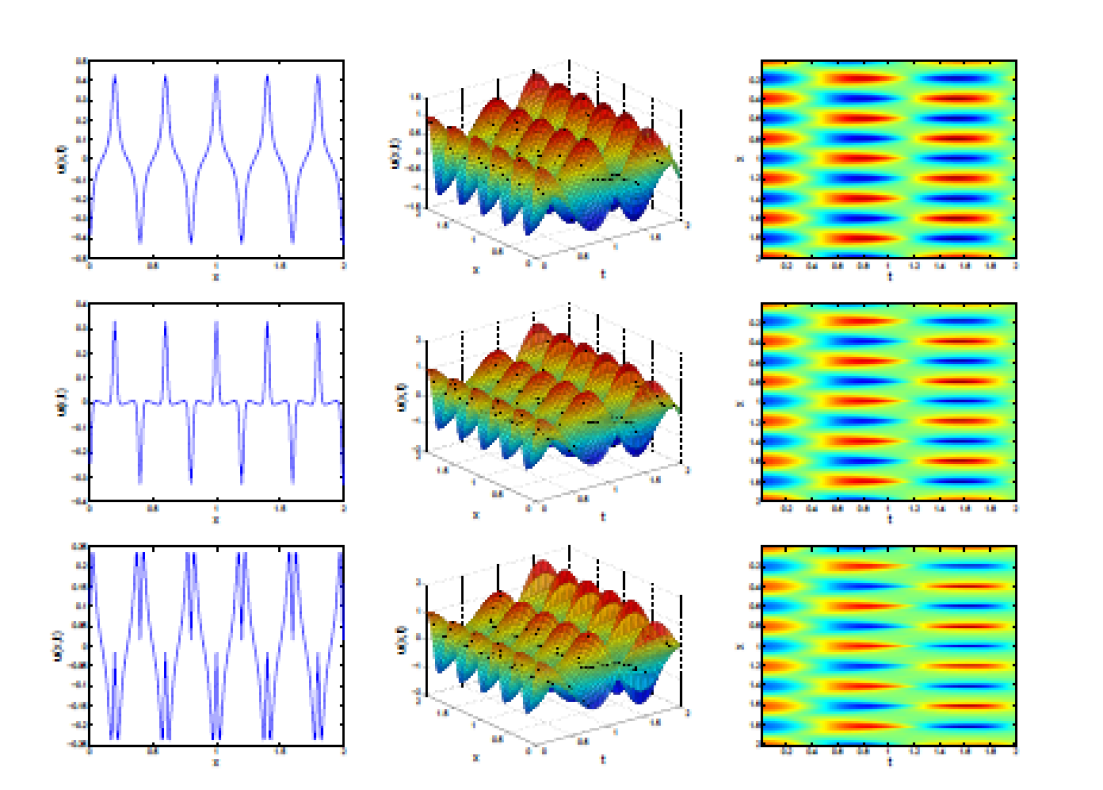
Figure 1: Spatial evolution of fractional Fisher’s equation (4.45) obtained at $\delta=0.1,\alpha=0.35,\tau=1.0,t=2$ for different derivatives. The upper-, middle- and lower-rows correspond to the Caputo, Caputo-Fabrizio and the Atangana-Baleanu derivatives respectively.

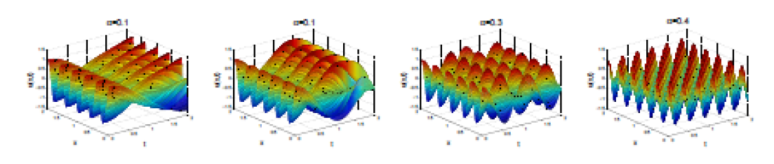
Figure 2: One-dimensional results showing the distribution of $u(x,t)$ at different instances of $\alpha=0.1(0.1)0.4$ for $t=1$. Other parameters are given in Figure 1.

Figure 3: Results showing the effects of time $t$ (upper-row) and spatial domain $L$ (lower-row) Other parameters are given in Figure 1.

For the second experiment, we simulate equations (4.45-4.47) on a spatial domain $\Omega\in[0,L]$, for $L>0$ with $\Delta t=0.25$, $\Delta x=0.5$ and $\tau=0.9$ with $N=200$. In Figure 1, we demonstrate the behaviours of the fractional derivatives for $\alpha=0.35$. The upper, middle and lower rows correspond to the Caputo, Caputo-Fabrizio and Atangana-Baleanu fractional derivatives. Merely looking at the figures, one may conclude that the three derivatives yielded a similar results. But a keen look will observe that they are not similar, column-1 of Figure 1 is a proof to this assertion.

The effects of fraction index $\alpha$ is observed in Figure 2 with the Caputo derivative. Likewise in Figure 3 (upper-row), we examined the distribution of $u(x,t)$ at some instances of final simulation time $t$. As the time is increasing so also the number of oscillations. In the lower panels, we observed the effects of increasing the domain size $L$, different patterns are obtained. It should be noted that other structures such as pure-spots, stripe and spatiotemporal patterns apart from what is reported in this work can be obtained, depending on how parameter values are chosen.

5 Conclusion

This paper has proposed the correct version of the fractional Adams-Bashforth methods which take into account the nonlinearity of the kernels including the power law for the Riemann-Liouville type, the exponential decay law for the Caputo-Fabrizio case and the Mittag-Leffler law for the Atangana-Baleanu scenario. The stability, as well as convergence results for each of the derivatives, are clearly presented. We compute the maximum norm error to check the performances of these schemes via the fractional Fisher’s equation at some instances of fractional-order $\alpha$. Formulation of space fractional Adams-Bashforth scheme with the Caputo, Caputo-Fabrizio and Atangana-Baleanu Riemann-Liouville derivatives, as well as their applications to real life problems are left for future research.

References

- [1] A. Atangana, On the new fractional derivative and application to nonlinear Fisher’s reaction-diffusion equation, Applied Mathematics and Computation, 273 (2016) 948-956.
- [2] A. Atangana, R.T. Alqahtani, Numerical approximation of the space-time Caputo-Fabrizio fractional derivative and application to groundwater pollution equation, Advances in Difference Equations, 2016(1) (2016) 1-13.
- [3] A. Atangana and D. Baleanu, New fractional derivatives with nonlocal and non-singular kernel: Theory and application to heat transfer model, Thermal Science, 20 (2016) 763-769.
- [4] D. Baleanu, R. Caponetto and J.T. Machado, Challenges in fractional dynamics and control theory, Journal of Vibration and Control, 22 (2016) 2151-2152.
- [5] M. Caputo and M. Fabrizio, A new definition of fractional derivative without singular kernel, Progress in Fractional Differentiation and Applications, 1 (2015) 73-85.
- [6] M. Caputo and M. Fabrizio, Applications of new time and spatial fractional derivatives with exponential kernels, Progress in Fractional Differentiation and Applications, 2 (2016) 1-11.
- [7] K. Dithelm, N.J. Ford and A.D. Freed, A predictor-corrector approach for the numerical solution of fractional differential equations, Nonlinear Dynamics, 29 (2002) 3-22.
- [8] J.F. Gómez-Aguilar. M.G. López-López, V.M. Alvarado-Martínez, J. Reyes-Reyes and M. Adam-Medina, Modeling diffusive transport with a fractional derivative without singular kernel, Physica A: Statistical Mechanics and its Applications, 447 (2016) 467-481.
- [9] J. F. Gómez-Aguilar and Abdon Atangana, New insight in fractional differentiation: power, exponential decay and Mittag-Leffler laws and applications, The European Physical Journal Plus, 132:13 (2017) DOI 10.1140/epjp/i2017-11293-3.
- [10] Analytical and numerical schemes for a derivative with filtering property and no singular kernel with applications to diffusion, The European Physical Journal Plus, (2016) 131:269. DOI 10.1140/epjp/i2016-16269-1
- [11] C.P. Li and Y.H. Wang, Numerical algorithm based on Adomian decomposition for fractional differential equations, Computers and Mathematics with Applications, 57 (2009) 1672-1681.
- [12] C.P. Li, A. Chen and J.J. Ye, Numerical approaches to fractional calculus and fractional ordinary differential equation, Journal of Computational Physics, 230 (2011) 3352-3368.
- [13] J. Losada and J. J. Nieto, Properties of the new fractional derivative without singular kernel, Progress in Fractional Differentiation and Applications, 1 (2015) 87-92.
- [14] K.S. Miller and B. Ross, An introduction to the fractional calculus and fractional differential equations, John Wiley & Sons Inc., New York, 1993.
- [15] S. Momani, Z. Odibat and V.S. Erturk, Generalized differential transform method for solving a space- and time-fractional diffusion-wave equation, Physics Letters A 370 (2007) 379-387.
- [16] K.M. Owolabi, Mathematical analysis and numerical simulation of patterns in fractional and classical reaction-diffusion systems, Chaos, Solitons and Fractals, 93 (2016) 89-98.
- [17] K.M. Owolabi and A. Atangana, Numerical solution of fractional-in-space nonlinear Schrödinger equation with the Riesz fractional derivative, The European Physical Journal Plus, (2016) 131: 335. DOI 10.1140/epjp/i2016-16335-8
- [18] K.M. Owolabi, Numerical solution of diffusive HBV model in a fractional medium, Springer Plus, (2016) 5:1643. DOI 10.1186/s40064-016-3295-x
- [19] K.M. Owolabi, Robust and adaptive techniques for numerical simulation of nonlinear partial differential equations of fractional order, Communications in Nonlinear Science and Numerical Simulation, 44 (2017) 304-317.
- [20] K. M. Owolabi and A. Atangana, Numerical approximation of nonlinear fractional parabolic differential equations with Caputo-Fabrizio derivative in Riemann-Liouville sense, Chaos, Solitons and Fractals, 99 (2017) 171-179.
- [21] K. M. Owolabi and A. Atangana, Numerical simulation of noninteger order system in subdiffussive, diffusive, and superdiffusive scenarios, Journal of Computational and Nonlinear Dynamics, 12 031010-1 (2017) 7-pages, DOI: 10.1115/1.4035195.
- [22] I. Petrás, Fractional-Order Nonlinear Systems: Modeling, Analysis and Simulation, Springer, Berlin 2011.
- [23] I. Podlubny, Fractional differential equations, Academic Press, New York, 1999.