A note on marginal correlation based screening

Abstract

Independence screening methods such as the two sample $t$-test and the marginal correlation based ranking are among the most widely used techniques for variable selection in ultrahigh dimensional data sets. In this short note, simple examples are used to demonstrate potential problems with the independence screening methods in the presence of correlated predictors. Also, an example is considered where all important variables are independent among themselves and all but one important variables are independent with the unimportant variables. Furthermore, a real data example from a genome wide association study is used to illustrate inferior performance of marginal correlation screening compared to another screening method.

Keywords and phrases. correlation, feature selection, screening, sure independence screening, two-sample t test

1 Introduction

Modern scientific research in diverse fields such as engineering, finance, genetics and neuroimaging involve data sets with hundreds of thousands of variables. For example, a typical problem in genetics is to study the association between a phenotype, say, resistance to a particular disease or yield of plants, and genotype involving millions of single nucleotide polymorphisms (SNP) markers. Nevertheless, only a few of these variables are believed to be important. Thus, variable selection plays a crucial role in modern scientific discoveries.

A variety of methods using different penalizations have been proposed for variable selection in the linear models, such as the Lasso (Tibshirani, 1996), SCAD (Fan and Li, 2001), elastic net (Zou and Hastie, 2005), adaptive Lasso (Zou, 2006) and others. These methods are very useful unless the number of predictors is much larger than the sample size (Wang, 2009; Fan et al., 2009). In the ultra-high dimensional set up, generally variable screening is performed to reduce the number of variables before applying any of the aforementioned variable selection methods for choosing important variables and estimation of the corresponding coefficients. One widely used variable screening procedure is based on marginal correlation or two-sample $t$ test (Li et al., 2012b; Fan and Lv, 2008). According to the review article of Saeys et al. (2007), “the two sample $t$-test and ANOVA are among the most widely used techniques in microarray studies” for feature selection. In particular, one popular method is to decide which variables should remain in the model based on ranking of marginal Pearson correlations (Fan and Lv, 2008). As mentioned in Fan and Lv (2008), (see also Fan et al., 2009; Cho and Fryzlewicz, 2012; Clarke and Clarke, 2018) there can be several potential issues with this method, although they are shown to have sure screening property (that is, with probability tending to one, important variables survive the screening) under certain conditions.

In this short note, through examples, we illustrate the problems with marginal correlation based screening in the presence of correlated predictors. In particular, assuming either autoregressive (order 1) or equicorrelation covariance structure for normally distributed predictor variables, it is shown that, with high probability, important variables do not survive such screening for linear regression models. We also consider an example where all important variables are independent among themselves and all but one important variables are independent with the entire set of unimportant variables. These examples are given in section 2. We also consider a real data example from an agricultural experiment in section 3 . For this high dimensional dataset, it is observed that the independence screening leads to both higher residuals and larger prediction errors than the high dimensional ordinary least squares projection (HOLP) screening method of Wang and Leng (2016). Finally, some concluding remarks are given in section 4.

2 Examples

Suppose the random vector $\mathbf{x}=(x_{1},\ldots,x_{p})^{\mathrm{T}}$ has a multivariate normal distribution with zero mean vector and covariance matrix $\mathbf{R}.$ Given $\mathbf{x}$ and a random variable $\epsilon\sim N(0,\sigma^{2})$ independent of $\mathbf{x}$, assume that

$$y=\beta_{0}+\boldsymbol{\beta}^{T}\mathbf{x}+\epsilon=\beta_{0}+\beta_{1}x_{1}+\cdots+\beta_{p}x_{p}+\epsilon,$$ (1)

where $\boldsymbol{\beta}\equiv(\beta_{1},\dots,\beta_{p})\in\mathbb{R}^{p}$ and all but a few $\beta_{i}$’s are zero.

In the following examples we shall show that given a covariance matrix $\mathbf{R},$ the nonzero $\beta_{i}$’s can take values that would make marginal correlation between $y$ and important variables smaller in magnitude than the same between $y$ and each of the unimportant variables. Indeed, in one example some of the important $x_{i}$’s become marginally uncorrelated with the response. We consider here two popular correlation structures. The first correlation structure is autoregressive where correlation between $x_{i}$ and $x_{j}$ is $\rho^{|i-j|}$ for some $\rho$ between 0 and 1. The second correlation structure is compound symmetric where the correlation between $x_{i}$ and $x_{j}$ is $\rho\in(0,1)$ whenever $i\neq j.$

The general setup of the simulations is as follows. We consider a particular multivariate Gaussian distribution for the random vector $\mathbf{x}$ and fix which of the $x_{i}$’s would have nonzero coefficients. Then for given value of the correlation parameter, we choose the values of the nonzero coefficients in such a way that some of those $x_{i}$’s become marginally uncorrelated with the response $y$ or have smaller marginal correlation (in absolute value) than that of the unimportant variables. Then we simulate $n$ independent realizations from the resulting joint model and compute all the sample correlations between $y$ and $x_{i}$, denoted as $w_{i},1\leq i\leq p.$ As mentioned in the introduction, a popular method of screening is to retain those features with largest absolute marginal correlations, that is, variables with $\lfloor n/\log(n)\rfloor$ or $\lfloor n^{1-\theta}\rfloor$ first largest $|w_{i}|$ values for some $0<\theta<1$ (Fan et al., 2009; Fan and Lv, 2008). In our simulation examples, we say a variable does not survive screening if its absolute marginal correlation is not among the largest $n$ of all. Based on these $w_{i}$’s, we observe if a particular subset of important variables survive screening or not. We repeat this process 100 times and report the proportion of times the important variables fail to survive screening.

Example 1

In this example, we consider the autoregressive correlation design and show using a simple example that an important variable may fail to survive screening based on its marginal correlation with the response. To this end, suppose the $(i,j)$th entry of $\mathbf{R}$ is $r_{ij}=\rho^{|i-j|}$ where $0<\rho<1.$ Note that the largest eigenvalue of $\mathbf{R}$ is bounded. Next, suppose $\boldsymbol{\beta}\in\mathbb{R}^{p}$ be such that $\beta_{j}=0$ if $j\notin\{1,3\}$ and

$$\begin{pmatrix}1&\rho^{2}\\ \rho&\rho\end{pmatrix}\begin{pmatrix}\beta_{1}\\ \beta_{3}\end{pmatrix}=\begin{pmatrix}0\\ a\end{pmatrix},$$

where $a\neq 0.$ Then, $\mathrm{Cov}(y,x_{1})=0$ even though $\beta_{1}\neq 0$ and $\mathrm{Cov}(y,x_{2})=a\neq 0$ even if $\beta_{2}=0.$ For a concrete example, suppose $\rho=1/4$ and $a=3,$ and $\sigma=1.$ Then the solutions are $\beta_{1}=-0.8$ and $\beta_{3}=12.8.$ For a given value of the sample size $n,$ we set $p=2n$ and generate data from the model (1) under the given setup. We repeat this process 100 times and obtain the proportion of times $x_{1}$ failed to survive the screening. In Table 1 we report these proportions for increasing values of $n.$ Clearly as $n\to\infty,$ variable $x_{1}$ does not survive screening based on marginal correlation with non-negligible probability.

In this example, the marginal correlation between $y$ and $x_{1}$ is exactly zero. In the next example, we consider the equicorrelation matrix and demonstrate that the important variables fail to survive screening even if the marginal correlations between $y$ and each of the important variables are bounded away from zero.

Table 1: Proportion of times $x_{1}$ failed to survive screening in Example 1.

$n$	50	200	500	1000
proportion	0.56	0.45	0.44	0.62

Example 2:

Suppose $\mathbf{R}$ is the equicorrelation matrix with correlation parameter $\rho.$ That is, the $(i,j)$th element of $\mathbf{R}$ is $\rho$ if $i\neq j$ and $1$ if $i=j.$ Note that, the largest eigenvalue of $\mathbf{R}$ is $1+(p-1)\rho$ which is $O(n)$ if $p=O(n).$ Without loss, suppose $\beta_{i}\neq 0,$ for $i\leq 5$ and $\beta_{i}=0$ for $i>5.$ The covariance between $y$ and $x_{i}$ is

$$\mathrm{Cov}(y,x_{i})=\begin{cases}\beta_{i}+\rho\sum_{j\neq i}\beta_{j}&\textrm{ if }\beta_{i}\neq 0\\ \rho\sum_{j=1}^{5}\beta_{j}&\textrm{ if }\beta_{i}=0.\end{cases}$$

Then if we choose $\beta_{1},\ldots,\beta_{5}$ by solving the following system of linear equations

$$\begin{pmatrix}1&\rho&\rho&\rho&\rho\\ \rho&1&\rho&\rho&\rho\\ \rho&\rho&1&\rho&\rho\\ \rho&\rho&\rho&1&\rho\\ \rho&\rho&\rho&\rho&\rho\end{pmatrix}\begin{pmatrix}\beta_{1}\\ \beta_{2}\\ \beta_{3}\\ \beta_{4}\\ \beta_{5}\end{pmatrix}=\begin{pmatrix}a\\ a\\ a\\ a\\ b\end{pmatrix},$$

for some $a,b$ with $|a|<|b|$, then we have

$$\mathrm{Cov}(y,x_{i})=\begin{cases}a&\textrm{ if }i\leq 4\\ b&\textrm{ if }i>5.\end{cases}$$

Thus, although $\beta_{i}\neq 0$ ($i\leq 4$), the marginal correlations between $y$ and each $x_{i}$ ($i\leq 4$) are all equal but uniformly smaller in magnitude than $\mathrm{Cor}(y,x_{j}),j>5.$ Accordingly, based on a sample of size $n$ (where $n<<p$), the sample marginal correlation coefficients between $y$ and each of $x_{1},\ldots,x_{4}$ will be smaller in magnitude than the same between $y$ and each of the unimportant variables. Thus, with probability tending to one, $x_{1},\ldots,x_{4}$ will fail to survive screening with increasing $n$.

The following simulation study confirms the conclusion. We set $a=1,b=4,p=2n,$ $\rho=0.10$ and $\sigma^{2}=1.$ We consider $n=100,500$ and $1000$. In Table 2 (a) we report the proportion of those cases where a particular $x_{i}$ $(i\leq 4)$ failed to survive screening.

This example is high-dimensional because $p=2n$, but $p$ increases linearly with $n$. In Table 2 (b) we consider the above setup, except with $p=n^{2}$. We see that in this case, the probabilities of not surviving the screening increase to one much faster. In ultra-high-dimensional cases this problem is further exacerbated. However, in ultra-high dimensional problems, the largest eigenvalue of the covariance matrix $\mathbf{R}$ increases at a larger rate than it does in the $p=2n$ case.

Table 2: Proportion of times $x_{1},\ldots,x_{4}$ failed to survive screening in Example 2. Left: $p=2n$, Right: $p=n^{2}.$

(a) $p=2n$
$n$	$x_{1}$	$x_{2}$	$x_{3}$	$x_{4}$
100	0.68	0.61	0.59	0.54
500	0.83	0.86	0.90	0.92
1000	0.96	0.96	0.96	0.97

(b) $p=n^{2}$
$n$	$x_{1}$	$x_{2}$	$x_{3}$	$x_{4}$
25	0.95	0.98	0.96	0.98
50	0.98	0.96	0.97	0.98
100	1.00	1.00	1.00	0.97

Example 3:

Unlike the previous two examples, here we assume that covariates corresponding to nonzero $\beta_{i}$’s are independent. In particular, we assume

$$\mathbf{R}=\begin{pmatrix}\mathbf{I}_{4}&\mathbf{0}^{\top}\\ \mathbf{0}&\mathbf{R}_{1}\end{pmatrix},$$

where $\mathbf{I}_{4}$ is the $4\times 4$ identity matrix, $\mathbf{0}$ is the $(p-4)\times 4$ matrix of zeros, and $\mathbf{R}_{1}$ is the $(p-4)\times(p-4)$ equicorrelation matrix (mentioned in Example 2) with correlation parameter $\rho.$ Also, as in Example 2, $\beta_{i}\neq 0,$ for $i\leq 5$ and $\beta_{i}=0$ for $i>5.$ Note that, the largest eigenvalue of $\mathbf{R}$ is $1+(p-5)\rho.$ The covariance between $y$ and $x_{i}$ is

$$\mathrm{Cov}(y,x_{i})=\begin{cases}\beta_{i}&\textrm{ if }i\leq 5\\ \rho\beta_{5}&\textrm{ if }i>5.\end{cases}$$

If $\beta_{i}$’s and $\rho$ are such that for $i\leq 4$, $|\beta_{i}|<|\rho\beta_{5}|$ then the marginal correlations between $y$ and $x_{i}$’s, $i\leq 4$ are all smaller in magnitude than $\mathrm{Cor}(y,x_{j}),j>5.$ Here, all the important covariates are independent among themselves and four out of the five true variables are independent with all covariates. But the dependence of exactly one of the true variables with the unimportant variables makes the marginal correlations for rest of the important variables uniformly smaller than those for the unimportant covariates. (This phenomenon may be termed as ‘nepotism effect’ here.) Thus with probability tending to one, $x_{1},\dots,x_{4}$ will fail to survive the marginal correlation screening with increasing $n$.

Next, we illustrate the performance of correlation screening using simulation with $\rho=0.2,\beta_{i}=1$ for $1\leq i\leq 4,\beta_{5}=10,\beta_{i}=0$ for $i\geq 6$ and $\sigma^{2}=1$. We consider the same $(n,p)$ values as in the Example 2. Based on 100 repetitions Table 3 provides the proportions of those cases where $x_{i}$ $(i\leq 4)$ failed to survive screening. As in Example 2, the probabilities of not surviving the screening increase to one faster when $p=n^{2}$ than when $p$ increases linearly with $n$.

Table 3: Proportion of times $x_{1},\ldots,x_{4}$ failed to survive screening. Left: $p=2n$, Right: $p=n^{2}.$

(a) $p=2n$
$n$	$x_{1}$	$x_{2}$	$x_{3}$	$x_{4}$
100	0.78	0.84	0.80	0.84
500	0.99	0.98	0.97	0.98
1000	1.00	1.00	1.00	1.00

(b) $p=n^{2}$
$n$	$x_{1}$	$x_{2}$	$x_{3}$	$x_{4}$
25	0.99	0.99	0.96	0.98
50	0.99	0.98	0.99	0.98
100	1.00	1.00	1.00	1.00

3 Real data example

We now study the performance of marginal correlation based screening in a real dataset. Cook et al. (2012) conducted a genome-wide association study on starch, protein, and kernel oil content in maize. The original field trial at Clayton, NC in 2006 consisted of more than 5,000 inbred lines and check varieties primarily coming from a diverse IL panel consisting of 282 founding lines (Flint-Garcia et al., 2005). However, marker information of only $N=3,951$ of these varieties are available from the panzea project (https://www.panzea.org/) which provide information on 546,034 SNPs after removing duplicates and SNPs with minor allele frequency (MAF) less than 5%. We use the phenotype oil content as our response for this analysis.

We randomly split the data into a training set of size $n=3,751$ and testing set of size 200. Using the training data we select the variables with large (absolute) marginal correlations. We consider three different screening model sizes, namely $\lfloor n/\log(n)\rfloor,\lfloor n^{1/2}\rfloor$ and $\lfloor n^{1/3}\rfloor$. Then linear models are fit using ordinary least-squares (OLS) with the selected variables from marginal correlation screening (Corr) and we compute the mean square errors (MSE) on the training dataset. Then we calculate the mean square prediction errors (MSPE) on the testing data based on the OLS fitted models. We also select variables using HOLP and consider the same three choices of the model size. Similarly, linear models are fit using the selected variables from the HOLP. The random splitting and the whole procedure is repeated 100 times. Figure  1 provides violin plots of the logarithm of MSE and MSPE values from these repetitions for both methods. In Figure  1 for the MSPE plot of independence screening with model size $\lfloor n/\log(n)\rfloor$, we have dropped an extreme outlier (about $60$) to obtain conspicuous MSE and MSPE violin plots for the HOLP. From Figure  1 we see that the independence screening leads to higher residuals as well as larger MSPEs than the HOLP. Finally, in Table 4 we report the median of the MSE and MSPE for each method corresponding to different selected model sizes. Table 4 also provides ratios of these median values, that is, $\mbox{med}(\mbox{MSE}_{\mbox{HOLP}})/\mbox{med}(\mbox{MSE}_{\mbox{Corr}})$ and $\mbox{med}(\mbox{MSPE}_{\mbox{HOLP}})/\mbox{med}(\mbox{MSPE}_{\mbox{Corr}})$. From these ratios we see that inaccuracies in terms of both model fit and prediction of the marginal correlation screening are exacerbated with increasing model size.

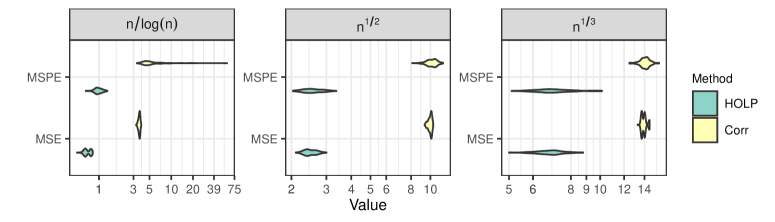
Figure 1: Violin plots of logarithm of MSE and MSPE values.

Table 4: Median MSE and MSPE for marginal correlation and HOLP screening.

Size	$\lfloor n^{1/3}\rfloor$			$\lfloor n^{1/2}\rfloor$			$\lfloor n/\log(n)\rfloor$
Method	HOLP	Corr	Ratio	HOLP	Corr	Ratio	HOLP	Corr	Ratio
MSE	6.89	14.00	0.49	2.46	10.02	0.25	0.67	3.63	0.18
MSPE	6.78	14.11	0.48	2.54	10.18	0.25	0.97	4.88	0.20

4 Conclusion

Here, we study performance of marginal correlation screening for the linear model with high dimensional data. Correlation ranking is one of the most widely used techniques for screening out unimportant features in genetics and other applied sciences. Using simulation and real data examples, we demonstrate several potential issues with the independent screening. Since the examples considered here are fairly simple, we hope that the article can serve the purpose of providing warning against the use of independence screening such as the two-sample $t$-test, and the marginal correlation ranking, without further investigation.

In the presence of nonlinear effects of the covariates on the response, although not considered in this article, the marginal correlation screening may miss the true variables (see e.g. Clarke and Clarke, 2018, Section 9.1). There are several alternatives to the Pearson correlation screening that have been proposed in the literature. Fan and Lv (2008) proposed the iterated sure independent screening. Various other correlation measures such as general correlation (Hall and Miller, 2009), distance correlation (Li et al., 2012b), rank correlation (Li et al., 2012a), tilted correlation (Cho and Fryzlewicz, 2012; Lin and Pang, 2014) and quantile partial correlation (Ma et al., 2017) have also been proposed to rank and screen variables. Thus users may compare the Pearson correlation rankings of their features with the selected variables from these iterative and other alternative correlations methods.

References

- Cho and Fryzlewicz (2012) Cho, H. and P. Fryzlewicz, 2012: High dimensional variable selection via tilting. Journal of the Royal Statistical Society, Series B, 74, no. 3, 593–622.
- Clarke and Clarke (2018) Clarke, B. S. and J. L. Clarke, 2018: Predictive Statistics: Analysis and Inference beyond Models. Cambridge University Press.
- Cook et al. (2012) Cook, J. P., M. D. McMullen, J. B. Holland, F. Tian, P. Bradbury, J. Ross-Ibarra, E. S. Buckler, and S. A. Flint-Garcia, 2012: Genetic architecture of maize kernel composition in the nested association mapping and inbred association panels. Plant Physiology, 158, no. 2, 824–834.
- Fan and Li (2001) Fan, J. and R. Li, 2001: Variable selection via nonconcave penalized likelihood and its oracle property. Journal of the American Statistical Association, 96, 1348–1360.
- Fan and Lv (2008) Fan, J. and J. Lv, 2008: Sure independence screening for ultrahigh dimensional feature space. Journal of Royal Statistical Society, Series B, 70, no. 5, 849–911.
- Fan et al. (2009) Fan, J., R. Samworth, and Y. Wu, 2009: Ultrahigh dimensional feature selection: beyond the linear model. Journal of Machine Learning Research, 10, 2013–2038.
- Flint-Garcia et al. (2005) Flint-Garcia, S. A., A.-C. Thuillet, J. Yu, G. Pressoir, S. M. Romero, S. E. Mitchell, J. Doebley, S. Kresovich, M. M. Goodman, and E. S. Buckler, 2005: Maize association population: a high-resolution platform for quantitative trait locus dissection. The Plant Journal, 44, no. 6, 1054–1064.
- Hall and Miller (2009) Hall, P. and H. Miller, 2009: Using generalized correlation to effect variable selection in very high dimensional problems. Journal of Computational and Graphical Statistics, 18, no. 3, 533–550.
- Li et al. (2012a) Li, G., H. Peng, J. Zhang, and L. Zhu, 2012a: Robust rank correlation based screening. Annals of Statistics, 40, no. 3, 1846–1877.
- Li et al. (2012b) Li, R., W. Zhong, and L. Zhu, 2012b: Feature screening via distance correlation learning. Journal of the American Statistical Association, 107, no. 499, 1129–1139.
- Lin and Pang (2014) Lin, B. and Z. Pang, 2014: Tilted correlation screening learning in high-dimensional data analysis. Journal of Computational and Graphical Statistics, 23, no. 2, 478–496.
- Ma et al. (2017) Ma, S., R. Li, and C.-L. Tsai, 2017: Variable screening via quantile partial correlation. Journal of the American Statistical Association, 112, no. 518, 650–663.
- Saeys et al. (2007) Saeys, Y., I. Inza, and P. Larrañaga, 2007: A review of feature selection techniques in bioinformatics. Bioinformatics, 23, 2507–2517.
- Tibshirani (1996) Tibshirani, R., 1996: Regression shrinkage and selection via the lasso. Journal of the Royal Statistical Society, Series B, 58, 267–288.
- Wang (2009) Wang, H., 2009: Forward regression for ultra-high dimensional variable screening. Journal of the American Statistical Association, 104, no. 488, 1512–1524.
- Wang and Leng (2016) Wang, X. and C. Leng, 2016: High dimensional ordinary least squares projection for screening variables. Journal of the Royal Statistical Society: Series B, 78, no. 3, 589–611.
- Zou (2006) Zou, H., 2006: The adaptive lasso and its oracle properties. Journal of the American Statistical Association, 101, 1418–1429.
- Zou and Hastie (2005) Zou, H. and T. Hastie, 2005: Regularization and variable selection via the elastic net. Journal of the Royal Statistical Society, Series B, 67, 301–320.