Signal tracking beyond the time resolution of an atomic sensor by Kalman filtering

Abstract

We study causal waveform estimation (tracking) of time-varying signals in a paradigmatic atomic sensor, an alkali vapor monitored by Faraday rotation probing. We use Kalman filtering, which optimally tracks known linear Gaussian stochastic processes, to estimate stochastic input signals that we generate by optical pumping. Comparing the known input to the estimates, we confirm the accuracy of the atomic statistical model and the reliability of the Kalman filter, allowing recovery of waveform details far briefer than the sensor’s intrinsic time resolution. With proper filter choice, we obtain similar benefits when tracking partially-known and non-Gaussian signal processes, as are found in most practical sensing applications. The method evades the trade-off between sensitivity and time resolution in coherent sensing.

Introduction.—Extremely precise sensors, e.g., atomic clocks Ludlow et al. (2015), magnetometers Kominis et al. (2003), and gravitational-wave detectors LIGO Scientific Collaboration and Virgo Collaboration (2016) employ a two-stage transducing architecture. A quantity of interest, e.g., electromagnetic field or gravitational-wave strain, coherently drives a well-isolated sensing component, e.g., the suspended mirrors of an interferometer or the spins of an atomic ensemble. The sensing component is non-destructively measured or “read out” by a second, meter component, often an optical beam. The two-stage architecture isolates the sensor component, enabling high coherence and high sensitivity Kominis et al. (2003), but also complicates the signal interpretation. In atomic sensors, for example, the slow spin-response, as well as intrinsic noises in spin orientation and in the readout, can distort and mask the signal Shah et al. (2010).

One compelling application of such sensors is estimation of time-varying signals, e.g., gravitational LIGO Scientific Collaboration and Virgo Collaboration (2016) or biomagnetic events Sander et al. (2012). For this application, the central statistical problem is waveform estimation Tsang (2009); Tsang et al. (2011). In control applications Geremia et al. (2004); Yonezawa et al. (2012); Wieczorek et al. (2015), the estimation must also be performed in real time Hochberg et al. (2012); Lien et al. (2016), as when a spectroscopy signal is fed back to a local oscillator in an atomic clock Ludlow et al. (2015).

Tools from Bayesian statistics van Trees et al. (2013); van Trees and Bell (2007) provide a natural framework for waveform estimation with multi-stage sensors. Of particular interest is the Kalman filter (KF) that provides fast and causal estimation Kalman (1960); Kalman and Bucy (1961). For linear Gaussian models, KF estimates are moreover optimal (i.e., with minimum mean squared error) and provide a full statistical description of the waveform. Sophisticated methods extend the KF technique to more general problems van Trees and Bell (2007). Even when not optimal, the KF is often applied for its simplicity, versatility and controllability Durrant-Whyte and Bailey (2006); Cassola and Burlando (2012).

To date KFs have been experimentally implemented in optical sensors: to estimate the phase of a light beam Yonezawa et al. (2012), to track an external force applied to a mirror in a quantum-enhanced interferometer Iwasawa et al. (2013), and to estimate in real time the quantum state of an optomechanical oscillator Wieczorek et al. (2015). Application to atomic sensors promises to benefit applications in magnetometry Kominis et al. (2003); Lucivero et al. (2014), gyroscopy Kornack et al. (2005), gravimetry de Angelis et al. (2009), optical NMR Jiménez-Martínez et al. (2014), fundamental physics Smiciklas et al. (2011), and quantum communications Julsgaard et al. (2004). Here, we demonstrate KFs in an archetypal two-stage atomic sensor: an atomic spin ensemble read-out via the optical Faraday effect.

Using spin polarization by optical pumping we apply known waveforms, which enables us to compare the KF estimates against the true value of the signal. In this way we first verify the accuracy of the statistical model underlying the KF and a major expected benefit of the KF approach—optimal waveform estimation including signal components faster than the intrinsic temporal resolution of the sensor. We also study estimation of waveforms with dynamics only partially known to the observer. The optimality studied in prior works Yonezawa et al. (2012); Iwasawa et al. (2013); Wieczorek et al. (2015) is not present in this scenario van Trees et al. (2013), which includes many important sensing problems Sander et al. (2012); Alem et al. (2015); Bar-Shalom et al. (2004). For appropriately-constructed KFs, we nonetheless observe advantages in speed and sensitivity, making the KF attractive for general-purpose atomic sensing.

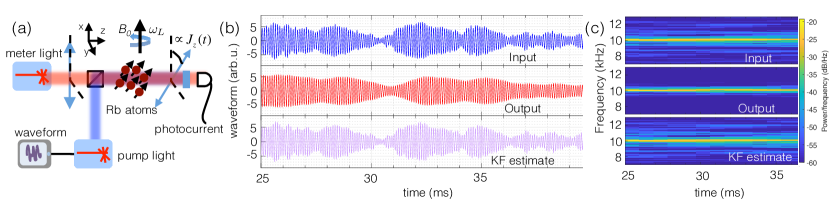
Figure 1: (a): An ensemble of ⁸⁷Rb atoms precesses at the Larmor frequency $\omega_{L}=2\pi\times$10\text{\,}\mathrm{kHz}$$ defined by an external magnetic field $B_{0}$. The spin $z$-component, $J_{z}(t)$, is driven by a circularly polarized light-beam (pump) carrying a waveform to be estimated. A second laser-beam (meter) is used for a polarimetry measurement producing a photocurrent that is proportional to $J_{z}(t)$ plus shot noise. Transmitted pump light is blocked by a dichroic filter (shown in blue). (b): A representative applied waveform (input) along with the corresponding measured photocurrent (output) and the recovered waveform (KF estimate). (c): Spectrograms of input, output and KF estimate showing that rapidly-varying features of the input are suppressed in the output yet are recovered in the KF estimate.

Two-stage sensor.—The sensor is depicted in Fig. 1(a). Its sensing component consists of an atomic ensemble exhibiting a total spin $J$, whose components $J_{i}(t)\!=\!\mathrm{Tr}\{\rho(t)\hat{J}_{i}\}$ with $i\in\{x,y,z\}$ are determined by the collective spin-operators, $\hat{J}_{i}$, and the ensemble state at time $t$, $\rho(t)$. The dynamics of $J$ includes: precession about $x$ at the Larmor (angular) frequency $\omega_{L}$ due to a known magnetic field $B_{0}$, coupling to the drive signal $\mathcal{E}(t)$ applied using circularly polarized pump-light along $z$, as well as relaxation and noise processes associated with atomic collisions, optical depolarization and transit-time broadening (all effectively characterised by the $T_{2}$-parameter and stochastic fluctuations measured via noise spectroscopy Lucivero et al. (2016, 2017)). The $J_{z}(t)$ spin of the ensemble is read out by the meter component of the sensor—a linearly-polarized off-resonance light beam propagating along $z$—which experiences Faraday rotation by an angle proportional to $J_{z}(t)$ yielding the detected photocurrent $I(t)$ subject to shot noise.

As shown in Fig. 1(b), rapidly-varying features in an applied waveform appear distorted in the output, due to the slow response of the atoms. See, e.g., the dip at $30.5\text{\,}\mathrm{ms}$, which appears only after a delay of $\approx\!$0.5\text{\,}\mathrm{ms}$$ with considerable loss of fast features. Despite this, a KF (described below) tracks these features as they occur in real time. To achieve these results the KF relies on a statistical model for spin, waveform, and detection dynamics.

Statistical model.—We describe the dynamics of the spin components $\mathbf{j}_{t}=[J_{y}(t),J_{z}(t)]^{T}$ using the linear Gaussian model of Refs. Lucivero et al. (2016, 2017), which after translating from frequency to time domain reads:

$$\mathrm{d}\mathbf{j}_{t}=\begin{bmatrix}-\frac{1}{T_{2}}&\omega_{\mathrm{L}}\\ -\omega_{\mathrm{L}}&-\frac{1}{T_{2}}\end{bmatrix}\mathbf{j}_{t}\,\mathrm{d}t+\begin{bmatrix}0\\ \mathcal{E}(t)\end{bmatrix}\mathrm{d}t+\mathrm{d}\mathbf{w}_{t}^{(\mathrm{J})},$$ (1)

where the spin-noise vector $\mathrm{d}\mathbf{w}_{t}^{(\mathrm{J})}=[\mathrm{d}w_{y}(t),\mathrm{d}w_{z}(t)]^{T}$ describes independent stochastic increments $\mathrm{d}w_{\alpha}(t)=\sqrt{Q_{\alpha}}\mathrm{d}W_{\alpha}(t)$ ($\alpha\in\{y,z\}$) obeying Gaussian white-noise statistics that we denote using the normal distribution $\mathrm{d}w_{\alpha}(t)\sim\mathcal{N}(0,Q_{\alpha}\mathrm{d}t)$ with mean $\mathrm{E}\!\left[\mathrm{d}w_{\alpha}(t)\right]=0$ and variance $\mathrm{E}\!\left[\mathrm{d}w_{\alpha}(t)\mathrm{d}w_{\beta}(t)\right]=\delta_{\alpha\beta}Q_{\alpha}\mathrm{d}t$, where the scalar strength $Q_{\alpha}>0$ is determined experimentally (see sup ).

The signal in (1), $\mathcal{E}(t)=[g_{\textrm{P}}\cos(\omega_{\mathrm{P}}t),g_{\textrm{P}}\sin(\omega_{\mathrm{P}}t)]\cdot\mathbf{q}_{t}$, contains the quadrature components $\mathbf{q}_{t}=[q(t),p(t)]^{T}$ that we aim to estimate, while the carrier-frequency $\omega_{\mathrm{P}}$ and coupling constant $g_{\textrm{P}}$ are known parameters sup . In the validation experiment of this work, we drive the atoms with a signal whose quadratures are described by independent Ornstein-Uhlenbeck (OU) processes Gardiner (1985) with correlation time $\kappa^{-1}$:

$$\mathrm{d}\mathbf{q}_{t}=-\kappa\,\mathbf{q}_{t}\mathrm{d}t+\mathrm{d}\mathbf{w}_{t}^{(\mathrm{q})},$$ (2)

where $\mathrm{d}\mathbf{w}_{t}^{(\mathrm{q})}=[\mathrm{d}w_{q}(t),\mathrm{d}w_{p}(t)]^{T}$ denotes the noise vector of the quadrature components containing independent stochastic increments that are defined in an analogous manner to the spin-noise vector in Eq. (1).

We monitor the atomic spins via optical Faraday rotation of the meter beam sup . As discussed in previous works Lucivero et al. (2016, 2017), the photocurrent $I(t)$ produced by this detection process is subjected to Gaussian white-noise of the light (i.e., optical shot noise). In our experiments we sample the photocurrent at finite-time intervals, i.e., at $t_{k}\!=\!k\,\Delta$ with integer $k$ and sampling period $\Delta$. To account for this fact, we describe the sensor output by a discrete-time stochastic equation of the form sup :

$$I(t_{k})=g_{\textrm{D}}\,J_{z}(t_{k})+\xi_{\mathrm{D}}(t_{k}),$$ (3)

where $g_{\textrm{D}}$ denotes the transduction constant in our experimental setup and $\xi_{\mathrm{D}}(t_{k})\sim\mathcal{N}(0,R^{\Delta})$ represents the white-noise of each observation, with variance $R^{\Delta}=R/\Delta$ dictated by the power-spectral-density, $R$, of the optical shot-noise and the sampling period, $\Delta$.

Kalman Filter.—In state estimation problems, the goal is to construct an estimator $\tilde{\mathbf{x}}_{t}$, that optimally tracks the state $\mathbf{x}_{t}$ of a system which, despite possessing known dynamics, cannot be directly measured due to detection noise and its intrinsic fluctuations van Trees et al. (2013). For linear-Gaussian systems, the optimal estimator—minimising the mean squared error—is provided by the Kalman Filter (KF) Kalman (1960); Kalman and Bucy (1961). For time-continuous processes integration-based versions of the KF are favored, e.g., Kalman-Bucy filters Tsang et al. (2009). However, as the output of our sensor is sampled at discrete times, we focus on its continuous-discrete version Bar-Shalom et al. (2004); sup applicable to dynamics described by the general state-space model of linear systems Bar-Shalom et al. (2004):

$$\mathrm{d}\mathbf{x}_{t} =\mathbf{F}_{t}\mathbf{x}_{t}\mathrm{d}t+\mathrm{d}\mathbf{w}_{t},$$ (4)

$$\mathbf{z}_{k} =\mathbf{H}_{k}\mathbf{x}_{k}+\mathbf{v}_{k},$$ (5)

where $\mathbf{x}_{t}$ and $\mathbf{z}_{k}\equiv\mathbf{z}_{t_{k}}$ are the state and observation vectors describing the system and measurement processes, respectively. For the atomic sensor under study, we define the state vector $\mathbf{x}_{t}=\mathbf{j}_{t}\oplus\mathbf{q}_{t}$, so that the system dynamics encompasses the evolution of transversal spin-components and signal quadratures, i.e., Eqs. (1) and (2), respectively. The stochastic increment in Eq. (4) is then formed by a direct sum, $\mathrm{d}\mathbf{w}_{t}=\mathrm{d}\mathbf{w}_{t}^{(\mathrm{J})}\oplus\mathrm{d}\mathbf{w}_{t}^{(\mathrm{q})}$, of the corresponding spin- and quadrature-noise vectors and satisfies $\mathrm{E}\!\left[\mathrm{d}\mathbf{w}_{t}\right]=\mathbf{0}$, $\mathrm{E}\!\left[\mathrm{d}\mathbf{w}_{t}\mathrm{d}\mathbf{w}_{t}^{T}\right]=\mathbf{Q}\,\mathrm{d}t$ with $\mathbf{Q}=\mathrm{diag}\{Q_{y},Q_{z},Q_{q},Q_{p}\}$ being its $4\!\times\!4$ diagonal covariance matrix. An explicit expression for the matrix $\mathbf{F}_{t}$ applicable to our atomic sensor can be found in Ref. sup . The photocurrent (3), on the other hand, constitutes the (scalar) measurement model (5) with $\mathbf{z}_{k}\!\equiv\!z_{k}\!=\!I(t_{k})$, $\mathbf{H}_{k}\equiv\mathbf{H}=[0,g_{\textrm{D}},0,0]$, and $\mathbf{v}_{k}\!\equiv\!v_{k}\!=\!\xi_{\mathrm{D}}(t_{k})$.

In the continuous-discrete KF the estimate, $\tilde{\mathbf{x}}_{t}$, and its error covariance matrix, $\mathbf{\Sigma}_{t}=\mathrm{E}\!\left[(\mathbf{x}_{t}-\tilde{\mathbf{x}}_{t})(\mathbf{x}_{t}-\tilde{\mathbf{x}}_{t})^{T}\right]$, are constructed in a two-step procedure Jazwinski (1970); van Trees et al. (2013). First, their values at $t_{k}$, $\tilde{\mathbf{x}}_{k|k-1}$ and $\mathbf{\Sigma}_{k|k-1}$, are predicted conditioned on the previous instance, $\tilde{\mathbf{x}}_{k-1|k-1}$ and $\mathbf{\Sigma}_{k-1|k-1}$, as follows:

$$\tilde{\mathbf{x}}_{{k|k-1}} =\mathbf{\Phi}_{k,k-1}\tilde{\mathbf{x}}_{k-1|k-1},$$ (6)

$$\mathbf{\Sigma}_{k|k-1} =\mathbf{\Phi}{{}_{k,k-1}}\mathbf{\Sigma}_{k-1|k-1}\mathbf{\Phi}_{k,k-1}^{T}+\mathbf{Q}_{k}^{\Delta},$$ (7)

where $\mathbf{\Phi}_{k,k-1}$ is the transition matrix describing the solution of the dynamical model (4) Kalman (1960). $\mathbf{Q}_{k}^{\Delta}$ is then the effective covariance matrix of the system noise, $\mathbf{Q}$, that now adequately accounts for the finite sampling period, $\Delta$, of the measurement sup . Second, the update step is performed according to the rule:

$$\tilde{\mathbf{x}}_{k|k} =\tilde{\mathbf{x}}_{k|k-1}+\mathbf{K}_{k}\,\tilde{\mathbf{y}}_{k},$$ (8)

$$\mathbf{\Sigma}_{k|k} =\left(\openone-\mathbf{K}_{k}\mathbf{H}_{k}\right)\mathbf{\Sigma}_{k|k-1},$$ (9)

after computing the innovation $\tilde{\mathbf{y}}_{k}$ and the Kalman gain $\mathbf{K}_{k}$ that depend on the “fresh” observation $\mathbf{z}_{k}$, i.e.,

$$\tilde{\mathbf{y}}_{k}=\mathbf{z}_{k}-\tilde{\mathbf{z}}_{k},\qquad\mathbf{K}_{k}=\mathbf{\Sigma}_{k|k-1}\mathbf{H}_{k}^{T}\mathbf{S}_{k}^{-1},$$ (10)

where $\tilde{\mathbf{z}}_{k}=\mathbf{H}{{}_{k}}\tilde{\mathbf{x}}_{k|k-1}$ represents the KF estimate of the $k$th observation, whose precision is then quantified by the covariance matrix:

$$\mathbf{S}{{}_{k}}=\mathrm{E}\!\left[\tilde{\mathbf{y}}_{k}\tilde{\mathbf{y}}_{k}^{T}\right]=\mathbf{R}^{\Delta}+\mathbf{H}_{k}\Sigma_{k|k-1}\mathbf{H}_{k}^{T}.$$ (11)

The KF is initialised according to an a priori distribution that represents our prior knowledge about the system and fixes $\tilde{\mathbf{x}}_{0|0}\sim\mathcal{N}(\mathbf{\boldsymbol{\mu}}_{0},\mathbf{\Sigma}_{0})$. For time-invariant system and measurement dynamics Jazwinski (1970), the KF must reach a steady-state solution as $k\to\infty$ with all $\mathbf{\Sigma}_{k|k}$, $\mathbf{K}_{k}$, $\mathbf{S}_{k}$ converging to steady-state values $\mathbf{\Sigma}_{\mathrm{ss}}$, $\mathbf{K}_{\mathrm{ss}}$, $\mathbf{S}_{\mathrm{ss}}$, respectively sup .

Experiment.—A cylindrical cell, of length $3\text{\,}\mathrm{cm}$ and diameter $1\text{\,}\mathrm{cm}$, contains isotopically enriched ⁸⁷Rb vapor and 100 Torr of $\rm N_{2}$ buffer gas, with controlled temperature and magnetic environment Lucivero et al. (2016) to maintain alkali number density of $4.5\times 10^{12}\text{\,}\mathrm{c}\mathrm{m}^{-3}$ and $\omega_{L}=2\pi\times$10\text{\,}\mathrm{kHz}$$. Meter light from a distributed-Bragg reflector laser (DBR) is red-detuned by 60 GHz from the $\rm D_{1}$ absorption line, while a circularly polarized signal beam from a second DBR diode is tuned to the $\rm D_{2}$ line-edge. Signal and meter beams each have effective area of $0.016\text{\,}{\mathrm{cm}}^{2}$, overlap at a non-polarizing 50:50 beam splitter placed before the cell, and propagate along the $z$ axis. A dichroic high-pass optical filter, placed after the cell, blocks the transmitted $\rm D_{2}$ light while passing the $\rm D_{1}$ probe beam for polarization analysis. Sensor parameters $\{T_{2},Q_{y},Q_{z},R\}$ are found by spin noise spectroscopy Lucivero et al. (2016, 2017); sup . The target signal, in particular, its quadratures $\mathbf{q}_{t}$, is digitally synthesized using an arbitrary-waveform-generator and applied to the injection current of the signal-beam DBR diode, to produce a pumping rate $\mathcal{E}(t)$ Jimenez-Martinez et al. (2010).

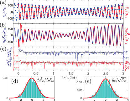
Figure 2: (a): Recorded sensor output ($z_{k}$, blue dots) along with its KF estimates ($\tilde{z}_{k}$, red solid line). The output is sampled at intervals $\Delta=$ $5\text{\,}\mathrm{\SIUnitSymbolMicro s}$; for clarity only even samples are shown. (b): Applied amplitude ($\mathcal{E}(t)$, blue) and its KF estimates ($\tilde{\mathcal{E}}_{k}$, red) shown in optical-rotation angle units scaled to the strength of detection shot-noise ($\sigma_{\mathrm{D}}=\sqrt{R^{\Delta}}$). (c): Corresponding behaviour of the true waveform estimation error squared ($\Delta^{2}\tilde{\mathcal{E}}_{k}$, blue line) and the innovations squared ($\tilde{y}_{k}^{2}$, red line), along with the variances predicted by the KF estimators (black solid lines) and Eqs. (9) and (11), respectively. (d-e): Histograms (cyan) of true signal-estimation error and innovations collected over a period of $15\text{\,}\mathrm{ms}$—as compared to the Gaussian PDFs predicted by the dynamical/observation models employed (red lines). All quantities plotted in (c-e) are renormalised to their asymptotic steady-state solutions.

Validation.—In the first experiment, the waveform $\mathcal{E}(t)$ is a single realization of the OU process described by Eq. (2) with $\kappa=$100\text{\,}\mathrm{s}^{-1}$$, see Fig. 1(b). A segment of the sensor output sequence, $z_{k}$, and the applied waveform, $\mathcal{E}_{k}$, are shown in Fig. 2(a-b), along with their KF estimates, $\tilde{z}_{k}$ and $\tilde{\mathcal{E}}_{k}=g_{\textrm{P}}(\tilde{q}_{k|k}\cos(\omega_{\mathrm{P}}t_{k})+\tilde{p}_{k|k}\sin(\omega_{\mathrm{P}}t_{k}))$. In Fig. 2(c), the square of the corresponding (single-shot) true estimation error, $\Delta^{2}\tilde{\mathcal{E}}_{k}=(\tilde{\mathcal{E}}_{k}-\mathcal{E}_{k})^{2}$, is plotted along with the (scalar) innovations squared, $\tilde{y}_{k}^{2}$. Note that consistently with the time-invariant linear-Gaussian model of (1)-(3) the estimates converge to their asymptotic steady-state solutions, i.e., to $\Delta^{2}\mathcal{E}_{\mathrm{ss}}=(\Sigma_{\mathrm{ss}}^{(q)})^{2}+(\Sigma_{\mathrm{ss}}^{(p)})^{2}$ and $S_{\mathrm{ss}}$ which we evaluate numerically sup . Furthermore, in order to fully validate the sensor model and the correctness of the KF implementation, we explicitly verify that the sequences of estimation errors $\Delta\tilde{\mathcal{E}}_{k}$ and $\tilde{y}_{k}$ are described by zero-mean Gaussian processes with variances dictated by Eqs. (9) and (11), respectively Bar-Shalom et al. (2004). In Fig. 2(d-e) we compare their histograms with the predicted distributions, and find that 94% (93%) of $\Delta\tilde{\mathcal{E}}_{k}$ ($\tilde{y}_{k}$) data points lie within a two-sided 95% confidence region of their respective predicted Gaussian distributions—indicating a very close agreement of the model and observed statistics.

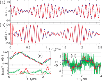
Figure 3: (a): Sensor output and; (b): applied waveform along with their respective KF estimates based on the polynomial model of Eq. (13); colors as in Fig. 2. (c, top):  Quadrature $\mathrm{bar}{q}(t)$ of the applied waveform (blue), in a single experimental run along with its KF estimates based on Wiener-process (WP, green) and polynomial (PM, red) models. (c, bottom, same colours):  Instantaneous bias (squared), $\text{Bias}(t)^{2}$, for the WP and PM estimators (obtained by averaging 6 experimental runs). The consistently delayed response to waveform variations of the WP model (visible comparing the blue and green curves), results in a higher bias of its KF estimate in (c), resulting then (after time-averaging) in a higher MSE shown in Table 1. (d): Time-derivative of the input waveform, $\dot{\mathrm{bar}{q}}(t)$, with its corresponding WP and PM estimates (same colours). As the WP estimators do not include the derivative, $\dot{\mathrm{bar}{q}}(t)$ can only be inferred from $\tilde{q}_{k}$, yielding the noisy green curve in (d).

Estimating unknown noisy waveforms.—The ultimate goal of waveform estimation is to track signals with dynamics partially known prior to the measurement Sander et al. (2012); Alem et al. (2015); Bar-Shalom et al. (2004). We now consider estimating waveforms whose quadrature vector $\mathbf{q}_{t}$ follows the quantity $\mathrm{bar}{\mathbf{q}}_{t}$ with unknown dynamics, but experiences fluctuations with known statistical properties $\mathrm{d}\mathbf{w}_{t}^{(\mathrm{q})}\sim\mathcal{N}(\mathbf{0},\mathbf{Q}^{(\mathrm{q})}\mathrm{d}t)$, so that:

$$\mathrm{d}\mathbf{q}_{t}=\dot{\mathrm{bar}{\mathbf{q}}}_{t}\mathrm{d}t+\mathrm{d}\mathbf{w}_{t}^{(\mathrm{q})}.$$ (12)

To study this scenario we synthesize waveforms with quadrature components $\mathrm{bar}{\mathbf{q}}(t)=[\mathrm{bar}{q}(t),0]$ and signal noise $\mathbf{Q}^{(\mathrm{q})}=\mathrm{diag}\{Q,Q\}$.We implement our filter with help of a (third-order) polynomial model Bar-Shalom et al. (2004); van Trees et al. (2013),, within which the evolution of the $q$-quadrature (and similarly for $p$) is modelled by the following dynamics sup :

$$\mathrm{d}q(t)=\dot{q}(t)\mathrm{d}t,~{}~{}\mathrm{d}\dot{q}(t)=\ddot{q}(t)\mathrm{d}t,~{}~{}\mathrm{d}\ddot{q}(t)=\mathrm{d}w^{(\ddot{\mathrm{q}})}_{t},$$ (13)

where the first and second derivatives are treated as a part of the waveform state space. The unknown deterministic and stochastic variations of the signal in Eq. (12) are then accounted for by introducing effective fluctuations of the $\ddot{q}(t)$-component, $\mathrm{d}w^{(\ddot{\mathrm{q}})}_{t}=\sqrt{Q/\Delta^{4}}\,\mathrm{d}W_{\ddot{q}}(t)$, with variance $\mathrm{d}w^{(\ddot{\mathrm{q}})}_{t}\mathrm{d}w^{(\ddot{\mathrm{q}})}_{t}=Q/\Delta^{4}\mathrm{d}t$. As a result, the enlarged quadrature-vector reads: $\mathbf{q}_{t}=[q_{t},\dot{q}_{t},\ddot{q}_{t};p_{t},\dot{p}_{t},\ddot{p}_{t}]^{T}$, and together with the spin degrees of freedom, $\mathbf{j}_{t}$, defines now the augmented state space. The KF is then used, as described before, to construct the estimator $\tilde{\mathbf{q}}_{k}$ with help of expressions found in Ref. sup for the corresponding discrete-time transition- and error-covariance-matrices.

The sensor output sequence $z_{k}$, applied waveform $\mathcal{E}_{k}$, and their respective KF estimates are shown in Fig. 3. Similarly to the case of the OU process depicted in Fig. 2, one observes the output to be distorted (i.e., smoothed and delayed) as compared to the applied waveform. Despite this, the filter tracks the salient features, amplitude and phase, of the waveform in real time. In Fig. 3(c-d), we show the true evolution of the quadrature $\mathrm{bar}{q}(t)$ and its time-derivative $\dot{\mathrm{bar}{q}}(t)$, respectively, along with the corresponding KF estimates $\tilde{q}_{k}$ and $\tilde{\dot{q}}_{k}$. We also compare the filter performance against its naïve implementation, which assumes the signal to be a pure Wiener process, i.e., $\mathrm{d}\mathbf{q}_{t}=\mathrm{d}\mathbf{w}_{t}^{(\mathrm{q})}$. Although the estimates based on the naïve implementation are less noisy, due to a smaller state space, they exhibit an intrinsic delay that cannot be compensated. The precision advantage of the polynomial model is summarised in Table 1, which shows that despite larger uncertainty (variance) the signal is tracked with much higher precision (smaller MSE) due to significant reduction of the bias. Moreover, by making the signal derivative a part of the state space, $\dot{\mathrm{bar}{q}}(t)$ can now be tracked in real time. In contrast, such information cannot be obtained using the naïve implementation of the filter—being masked out by the noise, see Fig. 3(d).

Model	$\text{Bias}^{2}$	Var	MSE
$\{\tilde{q}_{k}\}_{\mathrm{(WP)}}$	${3.36\times 10^{-5}}{}$	${3.0\times 10^{-6}}{}$	${3.66\times 10^{-5}}{}$
$\{\tilde{q}_{k}\}_{\mathrm{(PM)}}$	${1.02\times 10^{-5}}{}$	${7.6\times 10^{-6}}{}$	${1.78\times 10^{-5}}{}$

Table 1: Squared bias, variance (Var) and mean squared error (MSE) of the KF estimates, $\{\tilde{q}_{k}\}$, for the input quadrature, $\mathrm{bar}{q}(t)$, assuming the signal to be described by the Wiener process (WP) or the polynomial model (PM) of Eq. (13) and averaging over a time sequence of $15\text{\,}\mathrm{ms}$.

Conclusions.—We have demonstrated Kalman filtering in an archetypal two-stage atomic sensor. Driving the sensor with a known waveform, we have directly confirmed the validity of the statistical model describing the spin dynamics and the optical readout. Incorporating this model into the KF, we have demonstrated the optimal recovery of waveforms with spectral components far outside the intrinsic temporal resolution of the sensor. We have also shown how the same KF techniques can be efficiently employed to track waveforms with dynamics unknown prior to the measurement. These results may pave the way for employing KFs in a wide range of atomic sensing applications Kominis et al. (2003); Geremia et al. (2003); Kornack et al. (2005); de Angelis et al. (2009); Jiménez-Martínez et al. (2014); Smiciklas et al. (2011); Ludlow et al. (2015); Sander et al. (2012); Colangelo et al. (2017); Martin Ciurana et al. (2017).

Supplementary material for
R. Jiménez-Martínez et al. “Signal tracking beyond the time resolution of an atomic sensor by Kalman filtering”

Appendix A Optical detection of atomic spin and sensor characterisation

A.1 Faraday optical-rotation

Hyperfine coupling between the nuclear, $I$, and electronic, $S=1/2$, spins of an alkali atom splits its ground state into two hyperfine manifolds with total angular momentum: $f_{a}=I+1/2$ and $f_{b}=I-1/2$ (here, we set $\hbar\!=\!1$) Happer (1972). As a result, the Faraday optical-rotation angle $\Theta_{\mathrm{FR}}$ experienced by linearly-polarized off-resonance light propagating along the $z$ axis, and interacting with $N$ alkali atoms in the ground state, reads

$$\Theta_{\rm FR}=\frac{1}{2I+1}\left(g_{a}F_{a,z}-g_{b}F_{b,z}\right),$$ (14)

where $F_{\alpha,z}$ corresponds to the expectation value of the $z$-component of the collective spin of probed atoms associated with the hyperfine level $\alpha$, i.e., $F_{\alpha,z}\!=\!\textrm{Tr}\!\left\{\rho^{N}\sum_{k=1}^{N}{\hat{f}}^{(k)}_{\alpha,z}\right\}$ with $\rho^{N}$ being the ground-state density matrix describing the probed atomic ensemble, while ${\hat{f}}^{(k)}_{\alpha,z}$ represents the relevant angular momentum of the $k$th atom. In particular, as in our experiments the atoms are prepared in a coherent-spin state Happer (1972) that is separable and permutation invariant, i.e, $\rho^{N}=\varrho^{\otimes N}$, the collective spin operators for any $\alpha$th hyperfine level just linearly add, so that $F_{\alpha,z}\!=\!Nf_{\alpha,z}$ where $f_{\alpha,z}\!=\!\textrm{Tr}\!\left\{\varrho{\hat{f}}_{\alpha,z}\right\}$ stands for the mean angular momentum of each individual atom. Here, $N=nA_{\mathrm{eff}}L$ denotes the number of probed alkali atoms with $n$ being the alkali vapor density, $L$ is the path length of the light beam and $A_{\rm eff}$ its effective area Lucivero et al. (2016); Shah et al. (2010).

The hyperfine-coupling constant $g_{\alpha}$ in Eq. (14) is given by Happer (1972); Shah et al. (2010)

$$g_{\alpha}=\frac{c\,r_{\mathrm{e}}\,f_{\mathrm{osc}}}{A_{\rm eff}}\,\frac{\nu-\nu_{\alpha}^{\prime}}{(\nu-\nu_{\alpha})^{2}+(\Delta\nu_{\rm D1}/2)^{2}},$$ (15)

where $r_{\mathrm{e}}=2.82\times 10^{-13}$ cm is the classical electron radius, $f_{\mathrm{osc}}=0.34$ is the oscillator strength of the $\mathrm{D}_{1}$ transition in Rb, and $c$ is the speed of light. In Eq. (15), $\Delta\nu_{\rm D1}/2$ represents the pressure-broadened full-width at half-maximum (FWHM) of the $\mathrm{D}_{1}$ optical transition and $\nu-\nu_{\alpha}$ denotes the optical detuning of the probe-light. For our experimental conditions, i.e., alkali vapour cell filled with $100$ Torr of $\mathrm{N}_{2}$ buffer gas, $\Delta\nu_{\mathrm{light}}/2\approx$2.4\text{\,}\mathrm{GHz}$$. For a far-detuned probe-light beam, such that $|\nu-1/2\left(\nu_{a}+\nu_{b}\right)|>>|\nu_{a}-\nu_{b}|$, one can approximate $g_{a}\!\approx\!g_{b}$. Using the Wigner-Eckart theorem one obtains $j_{z}\!=\!\left(2I+1\right)^{-1}(f_{a,z}-f_{b,z})$ Biedenharn and Louck (1981). Thus, for the far-detuned light beam used in our experiments $\Theta_{\rm FR}$ can be approximated by

$$\Theta_{\rm FR}\approx\frac{c\,r_{\mathrm{e}}\,f_{\mathrm{osc}}}{A_{\rm eff}}\frac{1}{(\nu-\nu_{\alpha}^{\prime})}J_{z},$$ (16)

where $J_{z}=Nj_{z}=NP_{z}/2$ denotes the mean value of the collective spin along the $z$ direction, with the hyperfine structure ignored, with $P_{z}\in[-1,1]$ being the electronic spin polarization.

A.2 Detector photocurrent

To detect the optical rotation angle $\Theta_{\rm FR}$ of the meter light we use a balanced polarimeter consisting of a half-wave plate, polarization-beam-splitter, two balanced photodiodes and a low-noise transimpedance amplifier (TIA). The output of the TIA is given by $V_{\rm DPD}(t)=GI(t)$ with $G=$10^{6}\text{\,}\mathrm{V}\mathrm{/}{\mathrm{A}}$$ being the TIA gain and the photocurrent $I(t)$, which in the limit $\Theta_{\rm FR}\ll 1$ describing our experimental conditions is given by

$$I(t)\mathrm{d}t=2\Re P\Theta_{\rm FR}(t)\mathrm{d}t+\mathrm{d}w_{\rm sn}(t),$$ (17)

where $P=\int_{\cal A}dxdy\,{\cal I}(x,y)$ is the total power of the probe beam of area $\cal{A}=\rm A_{\rm eff}=$0.016\text{\,}{\mathrm{cm}}^{2}$$ reaching the detector with intensity profile ${\cal I}(x,y)$ and $\Re=$0.59\text{\,}\mathrm{A}\mathrm{/}\mathrm{W}$$ corresponds to the photodiode’s responsivity. In the first (second) experiment reported in the main manuscript $P=$500\text{\,}\mathrm{\SIUnitSymbolMicro W}$$ ($P=$100\text{\,}\mathrm{\SIUnitSymbolMicro W}$$). In Eq. (17), $\mathrm{d}w_{\rm sn}(t)=\sqrt{R}\mathrm{d}W$, where $\mathrm{d}W\sim\mathcal{N}(0,\mathrm{d}t)$ is the differential Wiener increment Gardiner (1985) and $R$ represents the intensity of the light shot-noise.

In our experiments the photocurrent $I(t)$ is sampled at a rate $\Delta^{-1}=$200\text{\,}\mathrm{k}\mathrm{S}\mathrm{a}\mathrm{-}\mathrm{s}$$. Thus, in order to correctly interpret the measurement outcomes, we need to formulate a discrete-time version of Eq. (17). Viewing the sampling process as a short-term average of the continuous-time measurement (c.f. Bar-Shalom et al. (2004)) the photocurrent $I(t_{k})$ recorded at $t_{k}\!=\!k\,\Delta$, with $k$ being an integer, can be expressed as

$$I(t_{k})=\frac{1}{\Delta}\int_{t_{k}-\Delta}^{t_{k}}I(t^{\prime})\mathrm{d}t^{\prime}=2\Re P\Theta_{\rm FR}(t_{k})+\frac{1}{\Delta}\int_{t_{k}-\Delta}^{t_{k}}\mathrm{d}w_{\rm sn}(t^{\prime}).$$ (18)

Hence, interpreting the last term above as an effective Langevin noise, i.e.,

$$\xi_{\mathrm{D}}(t_{k})\equiv\frac{1}{\Delta}\int_{t_{k}-\Delta}^{t_{k}}\mathrm{d}w_{\rm sn}(t^{\prime})$$ (19)

such that $R^{\Delta}:=\mathrm{E}\!\left[\xi_{\mathrm{D}}(t)\xi_{\mathrm{D}}(t)\right]=R/\Delta$, with $\Delta^{-1}$ quantifying the effective noise-bandwidth of each observation, and substituting for the Faraday optical-rotation angle according to Eq. (16), one finally arrives at Eq. (3) of the main text that describes the discrete-time detection process. The effective coupling constant $g_{\textrm{D}}$ in Eq. (3), which describes the (linear) transduction between the atomic spin and the photocurrent mediated by the meter light, then reads

$$g_{\textrm{D}}=2\Re P\frac{c\,r_{\mathrm{e}}\,f_{\mathrm{osc}}}{A_{\rm eff}}\frac{1}{(\nu-\nu_{\alpha}^{\prime})}.$$ (20)

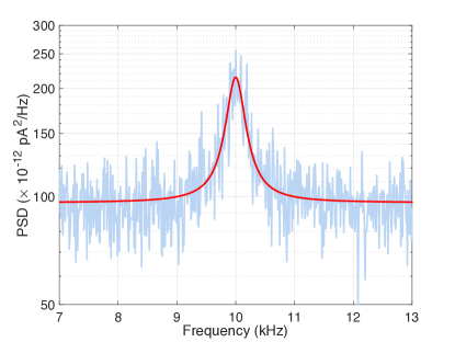
Figure 4: Noise spectroscopy of the meter signal Lucivero et al. (2016, 2017) used to characterize parameters $\{T_{2},Q_{y},Q_{z},R\}$. The averaging time of the shown spectrum corresponds to $50\text{\,}\mathrm{s}$ .

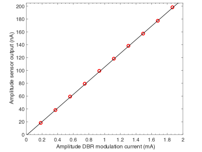
Figure 5: Linear response of atomic sensor output to a sinusoidal drive. The data points, shown in red, correspond to the observed sensor output obtained at a probe optical power $P=$100\text{\,}\mathrm{\SIUnitSymbolMicro W}$$. The solid line (in black) corresponds to a linear fit of the data. From the slope $b=$106.4\pm 0.4\text{\,}\mathrm{n}\mathrm{A}\mathrm{/}\mathrm{m}\mathrm{A}$$ of the linear fit we extract the effective coupling constant $g_{\textrm{P}}$ via $b=g_{\textrm{D}}g_{\textrm{P}}$.

A.3 Sensor characterization

We use noise spectroscopy of the meter signal (c.f. Lucivero et al. (2016, 2017)) to determine the sensor parameters $\{T_{2},Q_{y},Q_{z},R\}$. Fig. 5 shows a typical spectrum of the sensor output at the operating conditions of our experiment, yet in the situation when the pump beam is not coupled to the atomic ensemble.

The dynamical model of the atomic sensor—the spin dynamics and detection process described by Eqs. (1) and (3) of the main text, respectively—predicts the power spectrum, $S(\omega)$, to follow:

$$S(\omega)=S_{\mathrm{ph}}+\frac{S_{\mathrm{at}}}{(1/T_{2})^{2}+(\omega-\omega_{0})^{2}},$$ (21)

which we fit to the observed spectrum with the free parameters of the model being $\{S_{\mathrm{ph}},S_{\mathrm{at}},T_{2},\omega_{0}\}$ (see the red curve in Fig. 5), with $\omega_{0}=\omega_{L}$. From the fit we directly obtain the spin coherence time $T_{2}$ and straightforwardly determine the variance of the stochastic increments of the spin-noise vector $\mathrm{d}\mathbf{w}_{t}^{(\mathrm{J})}$ (see Eq. (1)), $g_{\textrm{D}}^{2}Q_{y}=g_{\textrm{D}}^{2}Q_{z}=2S_{\mathrm{at}}/T_{2}$, as well as the variance $R^{\Delta}=R/\Delta$ (with $R=S_{\mathrm{ph}}$) of the photon shot-noise (see Eq. (3)), following the methods described in Ref. Lucivero et al. (2016). Table 2 summarizes the values of the fitted model parameters.

Parameter	Value	Unit
$(2\pi T_{2})^{-1}$	$182\pm 4.1$	$\text{\,}\mathrm{Hz}$
$\omega_{0}/(2\pi)$	$9999.8\pm 2.9$	$\text{\,}\mathrm{Hz}$
$S_{\mathrm{at}}$	$118.7\pm 1.9$	$(\rm pA)^{2}/$\text{\,}\mathrm{H}\mathrm{z}$$
$S_{\mathrm{ph}}$	$96.0\pm 0.3$	$(\rm pA)^{2}/$\text{\,}\mathrm{H}\mathrm{z}$$

Table 2: Dynamical model parameters estimated from the spin-noise spectroscopy signal.

To calibrate the atomic response to the pump light beam we couple the pumping light to the ensemble and record the sensor output as a function of the amplitude of a resonant sinusoidal drive ($\omega_{P}=\omega_{L}=$10\text{\,}\mathrm{kHz}$$) applied to the injection current of the DBR pump-light laser. In Fig. 5 we plot the observed amplitude (red data points) of the sensor output as a function of the DBR current modulation, as well as a linear fit to the data (solid line). From the slope $b=$106.4\pm 0.4\text{\,}\mathrm{n}\mathrm{A}\mathrm{/}\mathrm{m}\mathrm{A}$$ of the linear fit we extract the effective coupling constant $g_{\textrm{P}}$.

Appendix B Kalman Filter as waveform estimator

In this appendix, we describe the construction of the Kalman Filter (KF)as the optimal waveform estimator for system and observation (measurement) linear-Gaussian dynamical models. We start by considering the continuous-continuous model, in which both the system and observations dynamics are described by continuous-time processes, and present the Kalman-Bucy Filter (KBF) that is then guaranteed to yield waveform estimates that minimise the mean squared error (MSE) at any time. We then consider the case of time-discrete observations, i.e., the continuous-discrete model, for which the optimal estimator is provided by the hybrid Kalman Filter (HKF) that we utilise in our experiment, as described in the main text. An interested reader is referred for more details to textbooks on classical filtering theory, e.g., by Jazwinski (1970) or van Trees et al. (2013).

B.1 Continuous-continuous model and the Kalman-Bucy Filter

B.1.1 Continuous system and measurement dynamics

Let us consider the case of system dynamics being described by a stochastic process with Gaussian noise, which formally corresponds to a time-varying Langevin equation (see, e.g., Gardiner (1985)) that dictates the evolution of the system state vector, $\mathbf{x}_{t}$, i.e., van Trees et al. (2013):

$$\frac{\mathrm{d}\mathbf{x}_{t}}{\mathrm{d}t}=\mathbf{F}_{t}\mathbf{x}_{t}+\mathbf{\Gamma}_{t}\mathbf{u}_{t}+\mathbf{G}_{t}\mathbf{w}_{t},$$ (22)

where $\mathbf{F}_{t}$, $\mathbf{\Gamma}_{t}$, $\mathbf{G}_{t}$ are generally time-dependent matrices, while $\mathbf{u}_{t}$ is a deterministically evolving vector, e.g., representing external force applied to the system. The initial conditions are fixed by specifying the mean state vector and its coviarance matrix at the initial time $t_{0}$, i.e., $\boldsymbol{\mu}_{0}:=\mathrm{E}\!\left[\mathbf{x}_{t_{0}}\right]$ and $\mathbf{\Sigma}_{\mathbf{x}_{t_{0}}}:=\mathrm{E}\!\left[\mathbf{x}_{t_{0}}\mathbf{x}_{t_{0}}^{T}\right]$, respectively, what then determines the initial Gaussian probability distribution of the state vector as $\mathbf{x}_{0}\sim\mathcal{N}(\boldsymbol{\mu}_{0},\mathbf{\Sigma}_{\mathbf{x}_{t_{0}}})$. On the other hand, the measurement outcomes are described by the observations vector, $\mathbf{z}_{t}$, which is assumed to be linearly related at all times to the state vector and to experience an independent stochastic Gaussian noise, i.e.:

$$\mathbf{z}_{t}=\mathbf{H}_{t}\mathbf{x}_{t}+\mathbf{v}_{t}$$ (23)

with the matrix $\mathbf{H}_{t}$ being again in principle time-dependent. In Eqs. (22) and (23), $\mathbf{w}_{t}$ and $\mathbf{v}_{t}$ denote the noise vectors—vectors with components consisting of stochastic (Wiener) white-noise terms Gardiner (1985)—such that for all $t$ and $s$:

$$\mathrm{E}\!\left[\mathbf{w}_{t}\right]=\mathrm{E}\!\left[\mathbf{v}_{t}\right]=0, \qquad\mathrm{E}\!\left[\mathbf{w}_{t}\mathbf{v}_{s}^{T}\right]=\mathrm{E}\!\left[\mathbf{v}_{t}\mathbf{w}_{s}^{T}\right]=0,$$ (24)

$$\mathrm{E}\!\left[\mathbf{w}_{t}\mathbf{w}_{s}^{T}\right]=\mathbf{Q}_{t}\,\delta(t-s), \qquad\mathrm{E}\!\left[\mathbf{v}_{t}\mathbf{v}_{s}^{T}\right]=\mathbf{R}_{t}\,\delta(t-s),$$ (25)

where $\mathbf{Q}_{t}$ and $\mathbf{R}_{t}$ are the noise (symmetric) covariance matrices that fully determine the properties of corresponding Gaussian fluctuations, i.e., $\mathbf{w}_{t}\sim\mathcal{N}\!\left(0,\mathbf{Q}_{t}\right)$ and $\mathbf{v}_{t}\sim\mathcal{N}\!\left(0,\mathbf{R}_{t}\right)$, and have a diagonal form, $\mathbf{Q}_{t}=\mathrm{diag}\!\left\{\{Q_{i}(t)\}_{i}\right\}$ and $\mathbf{R}_{t}=\mathrm{diag}\!\left\{\{R_{i}(t)\}_{i}\right\}$, assuming the distinct components of the noise vectors to be uncorrelated.

As the white-noise terms are ill-defined in the $\mathrm{d}t\to 0$ limit, in order to formally rewrite Eqs. (22) and (23) as stochastic differential equations, one must employ the Itō (or Stratonovich—not considered here) calculus, within which they read, respectively Gardiner (1985):

$$\mathrm{d}\mathbf{x}_{t} =\mathbf{F}_{t}\mathbf{x}_{t}{\mathrm{d}}t+\mathbf{\Gamma}_{t}\mathbf{u}_{t}{\mathrm{d}}t+\mathbf{G}_{t}\mathrm{d}\mathbf{w}_{t},$$ (26)

$$\mathrm{d}\mathbf{z}_{t} =\mathbf{H}_{t}\mathbf{x}_{t}{\mathrm{d}}t+\mathrm{d}\mathbf{v}_{t},$$ (27)

where now $\mathrm{d}\mathbf{w}_{t}=\{\sqrt{Q_{i}(t)}\mathrm{d}W_{i}(t)\}_{i}$ and $\mathrm{d}\mathbf{v}_{t}=\{\sqrt{R_{i}(t)}\mathrm{d}W_{i}(t)\}_{i}$ constitute vectors of Wiener increments, ${\mathrm{d}}W_{i}(t)$, which by the Itō rules must satisfy $\mathrm{d}W_{i}(t)\mathrm{d}W_{j}(t)=\delta_{ij}{\mathrm{d}}t$ and ${\mathrm{d}}W_{i}(t)^{2+k}={\mathrm{d}}W_{i}(t){\mathrm{d}}t=0$ for all $k>0$. Moreover, Eqs. (24) and (25) specifying the noise properties can then be rewritten in terms of the Itō differentials as:

$$\mathrm{E}\!\left[\mathrm{d}\mathbf{w}_{t}\right]=\mathrm{E}\!\left[\mathrm{d}\mathbf{v}_{t}\right]=0, \qquad\mathrm{E}\!\left[\mathrm{d}\mathbf{w}_{t},\mathrm{d}\mathbf{v}_{s}^{T}\right]=\mathrm{E}\!\left[\mathrm{d}\mathbf{v}_{t}\mathrm{d}\mathbf{w}_{s}^{T}\right]=0,$$ (28)

$$\mathrm{E}\!\left[\mathrm{d}\mathbf{w}_{t}\mathrm{d}\mathbf{w}_{s}^{T}\right]=\mathbf{Q}_{t}\,\delta(t-s)\,\mathrm{d}t, \qquad\mathrm{E}\!\left[\mathrm{d}\mathbf{v}_{t}\mathrm{d}\mathbf{v}_{s}^{T}\right]=\mathbf{R}_{t}\,\delta(t-s)\,\mathrm{d}t.$$ (29)

B.1.2 Estimator minimising the MSE given the observation record: the KBF

For given process (26) and observation (27) models, we would like to construct the most accurate estimate of the state vector at time $t$, i.e., $\mathbf{x}_{t}$, basing on the measurement record of all observations collected in the past, i.e., $\left\{\mathbf{z}_{\tau}\right\}_{\tau<t}$. Such an estimator may be formally defined as a random variable $\tilde{\mathbf{x}}_{t}:=f_{t}\!\left(\left\{\mathbf{z}_{\tau}\right\}_{\tau<t}\right)$ determined by some function $f_{t}$ that is designed to most efficiently interpret the observation record and predict $\mathbf{x}_{t}$ given particular dynamical models (26) and (27). Let us define for a given estimator the error covariance matrix that quantifies its deviation from the true state vector $\mathbf{x}_{t}$ at time $t$ as

$$\mathbf{\Sigma}_{t}:=\mathrm{E}\!\left[(\mathbf{x}_{t}-\tilde{\mathbf{x}}_{t})(\mathbf{x}_{t}-\tilde{\mathbf{x}}_{t})^{T}\right].$$ (30)

One seeks the optimal estimator minimising some figure of merit that quantifies the precision, i.e., the average distance of the estimator from the true state vector:

$$\textrm{Tr}\!\left\{\mathbf{W}\,\mathbf{\Sigma}_{t}\right\}=\mathrm{E}\!\left[(\mathbf{x}_{t}-\tilde{\mathbf{x}}_{t})^{T}\mathbf{W}(\mathbf{x}_{t}-\tilde{\mathbf{x}}_{t})\right],$$ (31)

where $\mathbf{W}$ is a weight matrix specifying contributions of each vector element to the overall estimation error. Choosing $\mathbf{W}=\openone$, in which case all vector components contribute equally, Eq. (31) simplifies to the mean squared error (MSE):

$$\mathrm{MSE}(t):=\textrm{Tr}\!\left\{\mathbf{\Sigma}_{t}\right\}=\mathrm{E}\!\left[(\mathbf{x}_{t}-\tilde{\mathbf{x}}_{t})^{T}(\mathbf{x}_{t}-\tilde{\mathbf{x}}_{t})\right]=\mathrm{E}\!\left[\left|\mathbf{x}_{t}-\tilde{\mathbf{x}}_{t}\right|^{2}\right].$$ (32)

Then, (see, e.g., Jazwinski (1970); van Trees et al. (2013)) by explicitly differentiating Eq. (32) with respect to $\tilde{\mathbf{x}}_{t}$, one may prove that the optimal estimator minimising the MSE is the mean of the posterior distribution $p(\mathbf{x}_{t+\delta t}|\left\{\mathbf{z}_{\tau}\right\}_{\tau<t})$, which describes the probability of system being in the state $\mathbf{x}_{t+\delta t}$ at time $t+\delta t$ given the past observation record $\left\{\mathbf{z}_{\tau}\right\}_{\tau<t}$. Hence, the optimal estimator at time $t+\delta t$ may always be formally written as

$$\tilde{\mathbf{x}}_{t+{\delta}t}=\int_{t}^{t+\delta t}\!\!\!D\mathbf{x}\;\mathbf{x}_{t+\delta t}\;p(\mathbf{x}_{t+\delta t}|\left\{\mathbf{z}_{\tau}\right\}_{\tau<t}),$$ (33)

where $\int_{t}^{t+\delta t}D\mathbf{x}$ denotes averaging over the fluctuations of the state vector occurring within the most recent interval, $[t,t+\delta t]$, after recording the last observation.

However, in the case of linear-Gaussian process and observation models—in particular, Eqs. (26) and (27)—such an optimal estimator can be shown to satisfy an ordinary differential equation, i.e., the Kalman-Bucy equation Kalman (1960); Kalman and Bucy (1961):

$$\frac{\mathrm{d}\tilde{\mathbf{x}}_{t}}{{\mathrm{d}}t}=\mathbf{F}_{t}\tilde{\mathbf{x}}_{t}+\mathbf{\Gamma}_{t}\mathbf{u}_{t}+\mathbf{K}_{t}\left(\mathbf{z}_{t}-\mathbf{H}_{t}\tilde{\mathbf{x}}_{t}\right),$$ (34)

where the term in brackets is known as the innovation, i.e.,

$$\tilde{\mathbf{y}}_{t}:=\mathbf{z}_{t}-\tilde{\mathbf{z}}_{t}\quad\text{with}\quad\tilde{\mathbf{z}}_{t}:=\mathbf{H}_{t}\tilde{\mathbf{x}}_{t}$$ (35)

representing then the effective estimate of the observation at time $t$, also provided by the estimator construction. The matrix $\mathbf{K}_{t}$ in Eq. (34) is the so-called Kalman gain:

$$\mathbf{K}_{t}:=\mathbf{\Sigma}_{t}\mathbf{H}_{t}^{T}\mathbf{R}_{t}^{-1},$$ (36)

which formally depends on the error covariance matrix $\mathbf{\Sigma}_{t}$ of the corresponding optimal estimator. Nevertheless, $\mathbf{K}_{t}$ may be determined independently of $\tilde{\mathbf{x}}_{t}$, as $\mathbf{\Sigma}_{t}$ can be shown to optimally fulfil the variance equation Kalman (1960); Kalman and Bucy (1961):

$$\frac{\mathrm{d}\mathbf{\Sigma}_{t}}{{\mathrm{d}}t}=\mathbf{F}_{t}\mathbf{\Sigma}_{t}+\mathbf{\Sigma}_{t}\mathbf{F}_{t}^{T}+\mathbf{G}_{t}\mathbf{Q}_{t}\mathbf{G}_{t}^{T}-\mathbf{\Sigma}_{t}\mathbf{H}_{t}^{T}\mathbf{R}_{t}^{-1}\mathbf{H}_{t}\mathbf{\Sigma}_{t},$$ (37)

which constitutes an example of matrix Riccatti (ordinary differential) equation that, despite being non-linear in $\mathbf{\Sigma}_{t}$, can always be efficiently solved, at least numerically Jazwinski (1970). Combined solutions to Eqs. (34) and (37) provide the optimal $\tilde{\mathbf{x}}_{t}$ as an integral of Eq. (34) over the observations $\mathbf{z}_{t}$ collected in the past. Such an estimator (which, however, often can only be computed numerically) is termed as the Kalman-Bucy filter (KBF) van Trees et al. (2013).

B.1.3 Steady-state solution of KBF

Under quite general conditions (see Ref. Kalman and Bucy (1961)) and, in particular, when dealing with time-invariant dynamical models (when the evolution models (26) and (27) are described by time-invariant $\mathbf{F}$, $\mathbf{G}$, $\mathbf{H}$, $\mathbf{R}$ and $\mathbf{Q}$), the solution of Eq. (37) must stabilize with time, so that $\mathrm{d}\mathbf{\Sigma}_{t}/\mathrm{d}t\to\mathbf{0}$ as $t\to\infty$. In such an asymptotic regime, the error covariance matrix approaches a constant matrix, i.e., the steady-state solution $\mathbf{\Sigma}_{\infty}$, for which the r.h.s. of Eq. (37) vanishes. Hence, $\mathbf{\Sigma}_{\infty}$ corresponds to the solution of the continuous algebraic Riccatti equation (CARE) van Trees et al. (2013),

$$\mathbf{0}=\mathbf{F}\mathbf{\Sigma}_{\infty}+\mathbf{\Sigma}_{\infty}\mathbf{F}^{T}+\mathbf{G}\mathbf{Q}\mathbf{G}^{T}-\mathbf{\Sigma}_{\infty}\mathbf{H}^{T}\mathbf{R}^{-1}\mathbf{H}\mathbf{\Sigma}_{\infty},$$ (38)

which then also determines the asymptotic value attained by the filter gain: $\mathbf{K}_{\infty}=\mathbf{\Sigma}_{\infty}\mathbf{H}^{T}\mathbf{R}^{-1}$. As Eq. (38) constitutes a matrix equation that is quadratic in $\mathbf{\Sigma}_{\infty}$, it is typically hard to find its analytical solution. However, efficient numerical methods are well-established, e.g., by employing the Schur decomposition method Laub (1979). Crucially, the steady-state solution, $\mathbf{\Sigma}_{\infty}$, quantifies the overall performance of the KBF—the minimal MSE (32), $\lim_{t\to\infty}\mathrm{MSE}(t)=\textrm{Tr}\!\left\{\mathbf{\Sigma}_{\infty}\right\}$, that may be attained for a particular continuous linear-Gaussian model (26-27) over large time-scales, i.e., when the waveform estimation procedure stabilises reaching its fundamental limits.

However, as in our atomic sensor experiment the measurements are taken at non-negligible time intervals—the sampling period $\Delta$ introduced in App. A.2—in what follows we must generalise the above derivation accounting explicitly for the time-discrete character of the observation model (27)—see Eq. (3) of the main text. Nevertheless, let us emphasize that the solutions obtained for such a time-discrete observation model must converge to the ones provided by the KBF and the CARE (38) in the limit of sufficiently frequent measurements, i.e., $\Delta\to 0$.

B.2 Continuous-discrete model and the Hybrid Kalman Filter

B.2.1 Continuous system but discrete measurement dynamics

When the measurements are performed in finite time-steps dictated by the sampling interval (period) $\Delta$, the observations must be formally described by a sequence of outcomes: $\left\{\mathbf{z}_{k}\right\}_{k=0}^{\left\lfloor t/\Delta\right\rfloor}$ with $t_{k}=k\Delta+t_{0}$ and $k\in\mathbb{N}$. Note that, for simplicity, we employ a notation in which any time-discrete quantity evaluated at time $t_{k}$ is labelled by the subscript $k$, e.g., $\mathbf{z}_{k}\equiv\mathbf{z}_{t_{k}}$. In such a time-discrete observation setting, the dynamics are described by a “hybrid” continuous-discrete model, in which the system evolves according to a time-continues process (26) while observations must be described employing the Langevin formulation (23):

$$\mathrm{d}\mathbf{x}_{t} =\mathbf{F}_{t}\mathbf{x}_{t}{\mathrm{d}}t+\mathbf{\Gamma}_{t}\mathbf{u}_{t}{\mathrm{d}}t+\mathbf{G}_{t}\mathrm{d}\mathbf{w}_{t},$$ (39)

$$\mathbf{z}_{k} =\mathbf{H}_{k}\mathbf{x}_{k}+\mathbf{v}_{k},$$ (40)

with the stochastic vector $\mathbf{v}_{k}\sim\mathcal{N}(0,\mathbf{R}_{k}^{\Delta})$ representing now, in contrast to time-continuous Eq. (23) with $\mathbf{v}_{t}\sim\mathcal{N}(0,\mathbf{R}_{t})$, a $k$-sequence defined by a discrete white-noise random process Gardiner (1985). Crucially, the Langevin term describing the observation noise fluctuates now with covariance $\mathbf{R}_{k}^{\Delta}:=\mathbf{R}_{t_{k}}/\Delta$, so that the observation model (40)consistently converges to Eq. (23) in the continuous measurement limit of $\Delta\to 0$ Bar-Shalom et al. (2004) (what then directly follows from Eq. (19)).

B.2.2 Estimator minimising the MSE given the observation record: the HKF

As discussed in the previous section, for any inference model the mean of the posterior distribution always constitutes the optimal estimator minimising the MSE. Hence, we may now formally define the optimal estimator by simply rewriting Eq. (33) and accounting for the time-discrete character of the observations:

$$\tilde{\mathbf{x}}_{k|k-1}=\int_{k-1}^{k}\!\!D\mathbf{x}\;\mathbf{x}_{k}\;p(\mathbf{x}_{k}|\left\{\mathbf{z}_{k^{\prime}}\right\}_{k^{\prime}=0}^{k-1}),$$ (41)

where $\int_{k-1}^{k}D\mathbf{x}\equiv\int_{t_{k-1}}^{t_{k}}D\mathbf{x}$ denotes now the averaging over the state fluctuations occurring during the $[t_{k-1},t_{k}]$ interval just before the $k$th observation is recorded. In the standard notation adopted above van Trees et al. (2013), $\tilde{\mathbf{x}}_{k|k-1}$represents the optimal estimator of the state vector at time $t_{k}$ given the past observation record $\left\{\mathbf{z}_{k^{\prime}}\right\}_{k^{\prime}=0}^{k-1}$, while $\tilde{\mathbf{x}}_{k|k}$ denotes the estimator at time $t_{k}$ that, however, has already been updated basing on the observation $\mathbf{z}_{k}$. Similar notation is used for the error covariance matrix (30) of $\tilde{\mathbf{x}}_{k|k-1}$ and $\tilde{\mathbf{x}}_{k|k}$, corresponding then to $\mathbf{\Sigma}_{k|k-1}$ and $\mathbf{\Sigma}_{k|k}$, respectively.

As the continuous-discrete model is described by Eqs. (39) and (40)that are still linear-Gaussian processes, the corresponding optimal estimator minimising the MSE is constructed in an analogous fashion to Eq. (33) defining the KBF, but in an explicit two-step prediction and update procedure Jazwinski (1970); van Trees et al. (2013) due to $\delta t\to 0$ limit being no longer valid in Eq. (41). Such a construction is then optimal, as due to lack of any outcome information in between the measurements the estimator within such time-intervals can only be evolved according to the system dynamics. At times $t_{k}=t_{0}+k\Delta$, on the other hand, it must be just updated basing on a particular outcome registered. Consequently, the optimal estimator is then called the hybrid Kalman filter (HKF) and it consistently converges to the KBF—the solution of (34)—in the $\Delta\to 0$ limit, in which the time-discrete Langevin equation (40) converges to its time-continuous form (23) Bar-Shalom et al. (2004).

Filter initialisation. Firstly, however, one must initialise the HKF at time $t_{0}$ after deciding on an appropriate initial Gaussian distribution, $p(\mathbf{x}_{0})\sim\mathcal{N}(\boldsymbol{\mu}_{0},\mathbf{\Sigma}_{\mathbf{x}_{0}})$, that adequately represents the knowledge about the state vector $\mathbf{x}_{0}\equiv\mathbf{x}(t_{0})$ prior to the estimation procedure. This corresponds to setting the initial HKF estimates of $\mathbf{x}_{0|0}$ and the covariance matrix $\mathbf{\Sigma}_{0|0}$ to, respectively:

$$\tilde{\mathbf{x}}_{0|0}=\int\mathrm{d}\mathbf{x}_{0}\,p(\mathbf{x}_{0})\,\mathbf{x}_{0}=:\boldsymbol{\mu}_{0},\qquad\mathbf{\Sigma}_{0|0}=\int\!\!\mathrm{d}\mathbf{x}_{0}\,p(\mathbf{x}_{0})\,\left(\mathbf{x}_{0}-\boldsymbol{\mu}_{0}\right)\left(\mathbf{x}_{0}-\boldsymbol{\mu}_{0}\right)^{T}=:\mathbf{\Sigma}_{\mathbf{x}_{0}}.$$ (42)

Here, we choose the Gaussian prior to be the distribution optimally inferred from a single observation $\mathbf{z}_{0}$ taken at the initial time $t_{0}$ Bar-Shalom et al. (2004). In particular, we set the mean to $\boldsymbol{\mu}_{0}=\mathbf{H}_{0}^{+}\mathbf{z}_{0}$, where $\mathbf{H}_{0}^{+}$ denotes the pseudoinverse of $\mathbf{H}_{0}$ in Eq. (40) at $t_{0}$, while the variance to $\mathbf{\Sigma}_{\mathbf{x}_{0}}=\mathbf{Q}_{0}+\mathbf{H}_{0}^{+}\mathbf{R}_{0}^{\Delta}(\mathbf{H}_{0}^{+})^{\rm T}$ in order to account for the uncertainty in filter initialisation due to intrinsic (unconditional) system and detection noises (determined by $\mathbf{Q}_{0}$ and $\mathbf{R}_{0}^{\Delta}$ of Eqs. (39) and (40), respectively).

Prediction step ($\tilde{\mathbf{x}}_{k-1|k-1}\to\tilde{\mathbf{x}}_{k|k-1}$ and $\mathbf{\Sigma}_{k-1|k-1}\to\mathbf{\Sigma}_{k|k-1}$). In order to perform the prediction step, let us define the transition matrix, $\mathbf{\Phi}$, as the solution of the non-stochastic part of the state-vector continuous dynamics (39) with also the deterministic term $\mathbf{u}_{t}$ being disregarded. In particular, we define $\mathbf{\Phi}_{t,s}$ (for a general time interval $[s,t]$) to be the matrix solution of

$$\frac{\mathrm{d}\mathbf{\Phi}_{t,s}}{{\mathrm{d}}t}=\mathbf{F}_{t}\mathbf{\Phi}_{t,s}$$ (43)

that must also satisfy $\mathbf{\Phi}_{\tau,\tau}=\openone$ for all $\tau\geq 0$. Hence, the transition matrix may be formally written as

$$\mathbf{\Phi}_{t,s}=\mathcal{T}_{\leftarrow}\exp\!\left[\int_{s}^{t}\mathrm{d}\tau\mathbf{F}_{\tau}\right]=\sum_{n=0}^{\infty}\frac{1}{n!}\,\mathbf{S}_{s,t}^{(n)}$$ (44)

where

$$\mathbf{S}_{s,t}^{(n)}:=\mathcal{T}_{\leftarrow}\int_{s}^{t}\!\!\int_{s}^{t_{1}}\!\!\!\dots\!\int_{s}^{t_{n-1}}\!\!\!\!\mathbf{F}_{t_{1}}\mathbf{F}_{t_{2}}\dots\mathbf{F}_{t_{n}}\,{\mathrm{d}}t_{1}{\mathrm{d}}t_{2}\dots\mathrm{d}t_{n}=\int_{s}^{t}\!\mathbf{F}_{t_{1}}\int_{s}^{t_{1}}\!\!\mathbf{F}_{t_{2}}\dots\int_{s}^{t_{n-2}}\!\!\!\!\mathbf{F}_{t_{n-1}}\int_{s}^{t_{n-1}}\!\!\!\!\mathbf{F}_{t_{n}}\,{\mathrm{d}}t_{n}{\mathrm{d}}t_{n-1}\dots\mathrm{d}t_{2}{\mathrm{d}}t_{1}.$$ (45)

$\mathcal{T}_{\leftarrow}$ in Eq. (44) denotes the time-ordering operation, as defined in Eq. (45), but may always be ignored in case the $\mathbf{F}$-matrices commute at different time-instances, i.e., when $\left[\mathbf{F}_{t},\mathbf{F}_{s}\right]=0$ for all $t$ and $s$. Moreover, in the case when the $\mathbf{F}$-matrix is time-independent, so that $\mathbf{\Phi}_{t,s}\equiv\mathbf{\Phi}_{t-s}=\mathrm{e}^{\mathbf{F}(t-s)}$, the transition matrix for any $\Delta$-interval $[t_{k-1},t_{k}]$ is the same and reads $\mathbf{\Phi}:=\mathbf{\Phi}_{\Delta}=\mathrm{e}^{\mathbf{F}\Delta}$.

With help of $\mathbf{\Phi}_{t,s}$, we can construct $\tilde{\mathbf{x}}_{k|k-1}$ as a function of $\tilde{\mathbf{x}}_{k-1|k-1}$ by integrating the estimator over the interval $[t_{k-1},t_{k}]$ according to the deterministic part of the system dynamics (39),

$$\tilde{\mathbf{x}}_{k|k-1}=\mathbf{\Phi}_{t_{k},t_{k-1}}\tilde{\mathbf{x}}_{k-1|k-1}+\int_{t_{k-1}}^{t_{k}}\mathbf{\Phi}_{t_{k},\tau}\mathbf{\Gamma}_{\tau}\mathbf{u}_{\tau}\mathrm{d}\tau,$$ (46)

while also adequately propagating the estimator covariance matrix:

$$\mathbf{\Sigma}_{k|k-1}=\mathbf{\Phi}_{t_{k},t_{k-1}}\mathbf{\Sigma}_{k-1|k-1}\mathbf{\Phi}_{t_{k},t_{k-1}}^{T}+\mathbf{Q}_{k}^{\Delta},$$ (47)

where

$$\mathbf{Q}_{k}^{\Delta}:=\int_{t_{k-1}}^{t_{k}}\mathbf{\Phi}_{t_{k},\tau}\mathbf{G}_{\tau}\mathbf{Q}_{\tau}\mathbf{G}_{\tau}^{T}\mathbf{\Phi}_{t_{k},\tau}^{T}\mathrm{d}\tau,$$ (48)

now represents the effective covariance matrix of the system noise, which importantly accounts for the finite sampling period, $\Delta$, of the time-discrete observation model (40) (see also Eq. (7) of the main text).

Note that the expression (46) for the predicted HKF constitutes the integral solution to the Kalman-Bucy equation (34) for the $[t_{k-1},t_{k}]$ interval with the observation-based updating completely ignored, i.e., the Kalman gain set to zero ($\mathbf{K}_{t}=\mathbf{0}$) in Eq. (34). Similarly, the error covariance matrix (47) of the prediction satisfies the variance equation (37) with the last term ignored, which in the case of the continuous-continuous model stood for the observation-based correction to the estimator.

Update step ($\tilde{\mathbf{x}}_{k|k-1}\to\tilde{\mathbf{x}}_{k|k}$ and $\mathbf{\Sigma}_{k|k-1}\to\mathbf{\Sigma}_{k|k}$). In order to incorporate into the estimator the $k$th outcome, $\mathbf{z}_{k}$, one simply adds to the prediction the $\mathbf{z}_{k}$-based innovation multiplied by the Kalman gain, i.e.,

$$\tilde{\mathbf{x}}_{k|k}=\tilde{\mathbf{x}}_{k|k-1}+\mathbf{K}_{k}\tilde{\mathbf{y}}_{k},$$ (49)

where the innovation and the Kalman gain now read, respectively:

$$\tilde{\mathbf{y}}_{k}=\mathbf{z}_{k}-\tilde{\mathbf{z}}_{k}\qquad\text{and}\qquad\mathbf{K}_{k}=\mathbf{\Sigma}_{k|k-1}\mathbf{H}_{k}^{T}\mathbf{S}_{k}^{-1}.$$ (50)

As before, $\tilde{\mathbf{z}}_{k}:=\mathbf{H}_{k}\tilde{\mathbf{x}}_{k|k-1}$ should be interpreted above as the filter-based prediction of the $k$th outcome value. For convenience, we have now explicitly defined the covariance matrix for the $k$th innovation $\tilde{\mathbf{y}}_{k}$ above as

$$\mathbf{S}{{}_{k}}:=\mathrm{E}\!\left[\tilde{\mathbf{y}}_{k}\tilde{\mathbf{y}}_{k}^{T}\right]=\mathbf{R}_{k}^{\Delta}+\mathbf{H}_{k}\mathbf{\Sigma}_{k|k-1}\mathbf{H}_{k}^{T},$$ (51)

whose behaviour, when explicitly computed and analysed for particular data, can also be utilised to verify the validity and accuracy of processes (39) and (40) describing the system and observation real dynamics Bar-Shalom et al. (2004) (see, in particular, Fig. 2(e) of the main text for the case the atomic sensor under study).

Finally, it is then straightforward to show that the estimator transformation (49) results in the following update of its error covariance matrix (30):

$$\mathbf{\Sigma}_{k|k}=\left(\openone-\mathbf{K}_{k}\mathbf{H}_{k}\right)\mathbf{\Sigma}_{k|k-1}$$ (52)

with the Kalman gain defined in Eq. (50).

B.2.3 Steady-state solution for the HKF

Similarly to the case of the KBF, when considering the continuous-discrete models but with time-invariant $\mathbf{F}$, $\mathbf{G}$, $\mathbf{H}$, $\mathbf{R}^{\Delta}$ and $\mathbf{Q}^{\Delta}$ in Eqs. (39) and (40) (for which then also $\mathbf{\Phi}=\mathrm{e}^{\mathbf{F}\Delta}$), the HKF approaches a steady-state solution as $k\to\infty$ van Trees et al. (2013). However, as the discrepancy between predicted and updated state values can be shown to be persistent also in the steady-state regime, one must define separately the constant values approached by the corresponding error covariance matrices for the prediction and update steps, respectively, as follows:

$$\mathbf{\check{\Sigma}}_{\mathrm{ss}}:=\lim_{k\to\infty}\mathbf{\Sigma}_{k|k-1}\qquad\text{and}\qquad\mathbf{\Sigma}_{\mathrm{ss}}:=\lim_{k\to\infty}\mathbf{\Sigma}_{k|k},$$ (53)

The form of $\mathbf{\check{\Sigma}}_{\mathrm{ss}}$ can be determined by substituting into Eq. (47) the expression for $\mathbf{\Sigma}_{k-1|k-1}$ according to Eq. (52), which then in the $k\to\infty$ limit (in which $\mathbf{\Sigma}_{k|k-1}\approx\mathbf{\Sigma}_{k-1|k-2}\,\to\,\mathbf{\check{\Sigma}}_{\mathrm{ss}}$) yields the discrete algebraic Riccatti equation (DARE), i.e., the equivalent of Eq. (38) for the continuous-discrete case van Trees et al. (2013):

$$\mathbf{\check{\Sigma}}_{\mathrm{ss}}=\mathbf{\Phi}\mathbf{\check{\Sigma}}_{\mathrm{ss}}\mathbf{\Phi}^{T}-\mathbf{\Phi}\mathbf{\check{\Sigma}}_{\mathrm{ss}}\mathbf{H}^{T}\left(\mathbf{R}^{\Delta}+\mathbf{H}\mathbf{\check{\Sigma}}_{\mathrm{ss}}\mathbf{H}^{T}\right)^{-1}\mathbf{H}\mathbf{\check{\Sigma}}_{\mathrm{ss}}\mathbf{\Phi}^{T}+\mathbf{Q}^{\Delta},$$ (54)

The asymptotically attained value $\mathbf{\check{\Sigma}}_{\mathrm{ss}}$ consequently allows us to compute the Kalman gain and the innovation covariance matrix for the steady-state regime, i.e.:

$$\mathbf{K}_{\mathrm{ss}}=\mathbf{\check{\Sigma}}_{\mathrm{ss}}\mathbf{H}^{T}\mathbf{S}_{\mathrm{ss}}^{-1}\quad\text{and}\quad\mathbf{S}_{\mathrm{ss}}=\mathbf{R}^{\Delta}+\mathbf{H}\mathbf{\check{\Sigma}}_{\mathrm{ss}}\mathbf{H}^{T},$$ (55)

so that the steady-state error covariance matrix for the update step can then be found using Eq. (52):

$$\mathbf{\Sigma}_{\mathrm{ss}}=\left(\openone-\mathbf{K}_{\mathrm{ss}}\mathbf{H}\right)\mathbf{\check{\Sigma}}_{\mathrm{ss}}.$$ (56)

Appendix C Applying the HKF to the atomic sensor

C.1 Continuous-discrete model describing the atomic sensor

The atomic sensor under study constitutes an example of the continuous-discrete dynamical model discussed in the previous section. In particular, the system evolution (39) describes the dynamics of both the ensemble spin-components transversal to the magnetic field $B_{0}$ (see Fig. 1 of the main text), $\mathbf{j}_{t}:=\left[J_{y}(t),J_{z}(t)\right]^{T}$, as well as the pump-beam quadratures, $\mathbf{q}_{t}:=\left[q(t),p(t)\right]^{T}$, representing the estimated waveform. Hence, in order to track the evolution, we construct the HKF for the state vector:

$$\mathbf{x}_{t}=\mathbf{j}_{t}\oplus\mathbf{q}_{t}=\left[\begin{array}[]{cc|cc}J_{y}(t)&J_{z}(t)&q(t)&p(t)\end{array}\right]^{T},$$ (57)

where, for convenience, we explicitly mark above the splitting of all the vectors and matrices into the relevant atomic-spin and quadrature parts. The stochastic-noise contribution in (39) is then given by the ${\mathrm{d}}\mathbf{w}_{t}$ term introduced in the main text below Eq. (2), which contains all the corresponding Wiener increments of atoms and light, i.e.,

$$\mathrm{d}\mathbf{w}_{t}={\mathrm{d}}\mathbf{w}_{t}^{(\mathrm{J})}\oplus{\mathrm{d}}\mathbf{w}_{t}^{(\mathrm{q})}=\left[\begin{array}[]{cc|cc}\sqrt{Q_{y}}{\mathrm{d}}W_{y}(t)&\sqrt{Q_{z}}\mathrm{d}W_{z}(t)&\sqrt{Q_{q}}\mathrm{d}W_{q}(t)&\sqrt{Q_{p}}\mathrm{d}W_{p}(t)\end{array}\right]^{T},$$ (58)

with noise intensity fully specified by the (diagonal) noise covariance matrix:

$$\mathbf{Q}=\mathbf{Q}^{(\mathrm{J})}\oplus\mathbf{Q}^{(\mathrm{q})}=\mathrm{diag}\left\{Q_{y},Q_{z}\right\}\oplus\mathrm{diag}\left\{Q_{q},Q_{p}\right\}.$$ (59)

Thus, the full dynamics of the state vector—encompassing both the evolution of the spin-ensemble as well as the stochastically driven quadratures (see Eqs. (1) and (2) of the main text, respectively)—corresponds to the special choice of the $\mathbf{F}$-matrix in Eq. (39):

$$\mathbf{F}_{t}=\left[\begin{array}[]{c|c}\mathbf{F}^{(\mathrm{J})}&\mathbf{F}_{t}^{(\mathrm{J\!\cdot\!q})}\\ \hline\cr\boldsymbol{0}&\mathbf{F}^{(\mathrm{q})}\end{array}\right]=\left[\begin{array}[]{cc|cc}-\frac{1}{T_{2}}&\omega_{\mathrm{L}}&0&0\\ -\omega_{\mathrm{L}}&-\frac{1}{T_{2}}&g_{\textrm{P}}\cos\!\left(\omega_{\mathrm{P}}t\right)&g_{\textrm{P}}\sin\!\left(\omega_{\mathrm{P}}t\right)\\ \hline\cr 0&0&-\kappa_{q}&0\\ 0&0&0&-\kappa_{p}\end{array}\right],$$ (60)

and, trivial, $\mathbf{\Gamma}_{t}=0$, $\mathbf{G}_{t}=\openone$.

On the other hand, the photocurrent detection described in Eq. (3) of the main text directly translates onto the time-discrete observation model (40) with the observation vector $\mathbf{z}_{k}$ being just a scalar representing the photocurrent measured at time $t_{k}$. In particular, the atomic-sensor setup corresponds then to just choosing in Eq. (40):

$$\mathbf{z}_{k}\equiv z_{k}=I(t_{k}),\quad\mathbf{v}_{k}\equiv v_{k}=\xi_{\mathrm{D}}(t_{k}),\quad\mathbf{H}_{k}\equiv\mathbf{H}=\left[\begin{array}[]{cc|cc}0&g_{\mathrm{D}}&0&0\end{array}\right],$$ (61)

and fixing the variance of the noise-term $v_{k}$ to the (scalar) intensity of the detection noise, i.e., $v_{k}\sim\mathcal{N}(0,R^{\Delta})$, so that consistently with Eq. (19) for all $k$ and $k^{\prime}$: $\mathrm{E}\!\left[v_{k}v_{k^{\prime}}\right]=\mathrm{E}\!\left[\xi_{\mathrm{D}}(t_{k})\xi_{\mathrm{D}}(t_{k^{\prime}})\right]=R^{\Delta}\,\delta_{kk^{\prime}}$.

Thanks to the above formulation we may directly apply the construction of the HKF described in the previous sections in order to optimally estimate the state vector (57). In particular, in accordance with the prescription of App. B.2.2, we first initialise the HKF at time $t_{0}$ with an initial (prior) Gaussian distribution $\tilde{\mathbf{x}}{{}_{0|0}}\sim\mathcal{N}(\mathbf{H}^{-1}\mathbf{z}_{0},\mathbf{Q}+\mathbf{H}^{-1}R^{\Delta}(\mathbf{H}^{-1})^{\rm T})$ after substituting for the predetermined (see App. A) experimental parameters in all the dynamical matrices. Then, at subsequent time-steps $k>0$, we apply the two-step recursive implementation of the HKF to construct the estimator $\mathbf{x}_{k|k}$ and covariance matrix $\mathbf{\Sigma}_{k|k}$ in an efficient manner, while constantly collecting the photocurrent experimental data $z_{k}$. The dynamical and noise parameters of the atomic sensor ($\omega_{\mathrm{L}}$, $T_{2}$, $g_{\mathrm{P}}$, $\omega_{\mathrm{P}}$, $\kappa_{p}$, $\kappa_{q}$, $\mathbf{u}_{t}$, $g_{\textrm{D}}$, $\mathbf{Q}$, $R^{\Delta}$) are either predetermined experimentally or pre-set and controlled by us, as discussed in the main text and App. A.

C.2 Steady-state solution for the HKF applicable to the atomic sensor

Let us note that in case of the atomic sensor under study all the dynamical matrices ($\mathbf{G}_{t}$, $\mathbf{\Gamma}_{t}$, $\mathbf{H}_{k}$) in Eqs. (39) and (40) are time-independent, with the only exception of $\mathbf{F}_{t}$, specified in Eq. (60). However, in the case of the experiment conducted, in which we set the signal quadratures to fluctuate according to white-noise of the same intensity, $Q_{q}=Q_{p}=:Q$, also the time-dependence of $\mathbf{F}_{t}$ can be bridged by moving to the “rotating frame” (RF) of the signal (pump) field which oscillates at the modulation frequency $\omega_{\mathrm{P}}$. Defining the corresponding transformation to the RF-picture (denoted by $\mathrm{bar}{\bullet}$) for any vector $\boldsymbol{\alpha}$ as

$$\mathrm{bar}{\boldsymbol{\alpha}}=\mathsf{R}_{\omega_{\mathrm{P}}t}\boldsymbol{\alpha}\qquad\text{with}\qquad\mathsf{R}_{\omega_{\mathrm{P}}t}:=\left[\begin{array}[]{cc}\cos\omega_{\mathrm{P}}t&\sin\omega_{\mathrm{P}}t\\ -\sin\omega_{\mathrm{P}}t&\cos\omega_{\mathrm{P}}t\end{array}\right],$$ (62)

we can rewrite the stochastic dynamics of the quadratures in the RF (stemming from the Eq. (2) of the main text) as

$$\mathrm{d}\mathrm{bar}{\mathbf{q}}_{t}=\left[\begin{array}[]{cc}-\kappa&\omega_{\mathrm{P}}\\ -\omega_{\mathrm{P}}&-\kappa\end{array}\right]\mathrm{bar}{\mathbf{q}}_{t}{\mathrm{d}}t+{\mathrm{d}}\mathrm{bar}{\mathbf{w}}_{t}^{(\mathrm{q})},$$ (63)

where all the vectors are rotated into the RF according to Eq. (62). Note that the covariance matrix of the quadrature-noise increments, ${\mathrm{d}}\mathrm{bar}{\mathbf{w}}_{t}^{(\mathrm{q})}$, remains unchanged, as

$$\mathrm{E}\!\left[{\mathrm{d}}\mathrm{bar}{\mathbf{w}}_{t}^{(\mathrm{q})}{\mathrm{d}}\mathrm{bar}{\mathbf{w}}_{t}^{(\mathrm{q})T}\right]=\mathsf{R}_{\omega_{\mathrm{P}}t}\left(\mathbf{Q}^{(\mathrm{q})}{\mathrm{d}}t\right)\mathsf{R}_{\omega_{\mathrm{P}}t}^{T}=\mathsf{R}_{\omega_{\mathrm{P}}t}\left(\mathrm{diag}\{Q,Q\}\right)\mathsf{R}_{\omega_{\mathrm{P}}t}^{T}{\mathrm{d}}t=\mathrm{diag}\{Q,Q\}\,{\mathrm{d}}t=\mathrm{E}\!\left[{\mathrm{d}}\mathbf{w}_{t}^{(\mathrm{q})}{\mathrm{d}}\mathbf{w}_{t}^{(\mathrm{q})T}\right].$$ (64)

Combining the RF-based quadrature dynamics (63) with the unaltered spin-ensemble evolution, we can write the modified dynamics of the full state vector (57) as

$${\mathrm{d}}\mathrm{bar}{\mathbf{x}}_{t}=\mathbf{F}_{\mathrm{RF}}\mathrm{bar}{\mathbf{x}}_{t}{\mathrm{d}}t+{\mathrm{d}}\mathrm{bar}{\mathbf{w}}_{t},$$ (65)

where:

$$\mathrm{bar}{\mathbf{x}}_{t}=\mathbf{j}_{t}\oplus\mathrm{bar}{\mathbf{q}}_{t},\quad\mathrm{bar}{\mathbf{u}}_{t}=\mathbf{u}_{t}^{(\mathrm{J})}\oplus\mathrm{bar}{\mathbf{u}}_{t}^{(\mathrm{q})},\quad{\mathrm{d}}\mathrm{bar}{\mathbf{w}}_{t}={\mathrm{d}}\mathbf{w}_{t}^{(\mathrm{J})}\oplus{\mathrm{d}}\mathrm{bar}{\mathbf{w}}_{t}^{(\mathrm{q})},$$ (66)

and the $\mathbf{F}$-matrix now reads in the RF:

$$\mathbf{F}_{\mathrm{RF}}:=\left[\begin{array}[]{cccc}-\frac{1}{T_{2}}&\omega_{\mathrm{L}}&0&0\\ -\omega_{\mathrm{L}}&-\frac{1}{T_{2}}&g_{\textrm{P}}&0\\ 0&0&-\kappa&\omega_{\mathrm{P}}\\ 0&0&-\omega_{\mathrm{P}}&-\kappa\end{array}\right],$$ (67)

being, indeed, time-independent. Finally, note that as the observation vector $z_{k}$, defined in Eq. (61) and representing the photocurrent measurement, is coupled only to the atomic-spin dynamics, the observation dynamical model remains unaffected by moving to the RF.

Crucially, in the RF picture, we can now write the corresponding DARE (54) for the atomic sensor, in order to determine the steady-state solution of the prediction-based error covariance matrix, $\mathbf{\check{\Sigma}}_{\mathrm{ss}}^{\mathrm{RF}}$, i.e.,

$$\mathbf{\check{\Sigma}}_{\mathrm{ss}}^{\mathrm{RF}}=\mathbf{\Phi}\mathbf{\check{\Sigma}}_{\mathrm{ss}}^{\mathrm{RF}}\mathbf{\Phi}^{T}-\mathbf{\Phi}\mathbf{\check{\Sigma}}_{\mathrm{ss}}^{\mathrm{RF}}\mathbf{H}^{T}\left(R^{\Delta}+\mathbf{H}\mathbf{\check{\Sigma}}_{\mathrm{ss}}^{\mathrm{RF}}\mathbf{H}^{T}\right)^{-1}\mathbf{H}\mathbf{\check{\Sigma}}_{\mathrm{ss}}^{\mathrm{RF}}\mathbf{\Phi}^{T}+\mathbf{Q}^{\Delta},$$ (68)

where the transition matrix reads $\mathbf{\Phi}_{t}=\mathrm{e}^{\mathbf{F}_{\mathrm{RF}}t}$, so that according to Eq. (48):

$$\mathbf{Q}^{\Delta}=\mathbf{\Phi}_{\Delta}\left(\int_{0}^{\Delta}\!\!\mathrm{d}\tau\mathbf{\Phi}_{-\tau}\mathbf{Q}\mathbf{\Phi}_{-\tau}^{T}\right)\mathbf{\Phi}_{\Delta}^{T},$$ (69)

while $\mathbf{Q}$, $\mathbf{H}$ and $\mathbf{F}_{\mathrm{RF}}$ are defined in Eqs. (59), (61) and (67), respectively. Consequently, the steady-state solution for the error covariance matrix after the update step, $\mathbf{\Sigma}_{\mathrm{ss}}^{\mathrm{RF}}$, is then determined by just substituting the solution of Eq. (68) into consecutively Eqs. (55) and (56).

Finally, note that all covariance matrices—in particular, the steady-state solutions—can then be computed in the laboratory frame by transforming back from the RF via $\mathbf{\Sigma}=\mathsf{R}_{\mathrm{\omega_{\mathrm{P}}t}}^{(\mathrm{q,J})}\mathbf{\Sigma}^{\mathrm{RF}}(\mathsf{R}_{\mathrm{\omega_{\mathrm{P}}t}}^{(\mathrm{q,J})})^{T}$, where $\mathsf{R}_{\mathrm{\omega_{\mathrm{P}}t}}^{(\mathrm{q,J})}:=\openone^{(\mathrm{J})}\oplus\mathsf{R}_{\mathrm{\omega_{\mathrm{P}}t}}$.

Appendix D Tracking unknown signals with polynomial models

In the final section of the appendix, we discuss how to construct KF-based estimators for waveforms of unknown average dynamics after approximating their behaviour by means of the so-called polynomial models and adequately augmenting the state space with waveform derivatives Bar-Shalom et al. (2004); van Trees et al. (2013). As discussed in the main text (see Eq. (12)), we are interested in estimating waveforms, $\mathbf{q}_{t}$, which follow unknown dynamics, $\mathrm{bar}{\mathbf{q}}_{t}$, and experience fluctuations of known statistical properties, $\mathrm{d}\mathbf{w}_{t}^{(0)}:=[\mathrm{d}w_{q}(t),\mathrm{d}w_{p}(t)]^{T}\sim\mathcal{N}(0,\mathbf{Q}\,\mathrm{d}t)$, so that in the Itō form:

$$\mathrm{d}\mathbf{q}_{t}=\mathrm{d}\mathrm{bar}{\mathbf{q}}_{t}+\mathrm{d}\mathbf{w}_{t}^{(0)}=\dot{\mathrm{bar}{\mathbf{q}}}_{t}\mathrm{d}t+\mathrm{d}\mathbf{w}_{t}^{(0)}.$$ (70)

Abusing the Itō notation and including higher orders of $\mathrm{d}t$, we explicitly Taylor-expand the differential $\mathrm{d}\mathrm{bar}{\mathbf{q}}_{t}$ as follows

$$\mathrm{d}\mathrm{bar}{\mathbf{q}}_{t}\approx\mathrm{bar}{\mathbf{q}}(t+\mathrm{d}t)-\mathrm{bar}{\mathbf{q}}(t)=\sum_{n=1}^{\infty}\frac{\mathrm{bar}{\mathbf{q}}_{t}^{(n)}}{n!}\mathrm{d}t^{n},$$ (71)

where $\mathrm{bar}{\mathbf{q}}_{t}^{(n)}:=\frac{\mathrm{d}^{n}\mathrm{bar}{\mathbf{q}}_{t}}{\mathrm{d}t^{n}}$ denotes the $n$th time-derivative of the signal at time $t$. By adopting the polynomial model one approximates the expansion (71) up to some order, $l$, and assumes the noise term, $\mathrm{d}\mathbf{w}_{t}^{(0)}$, to originate solely from fluctuations of $\mathrm{bar}{\mathbf{q}}_{t}^{(l)}$. In particular, the evolution of the state vector $\mathbf{q}_{t}$ is then modelled as the solution of the following set of $l+1$ coupled (stochastic) differential equations:

$$\begin{array}[]{crcl}n=0,&~{}\mathrm{d}\mathrm{bar}{\mathbf{q}}_{t}{}&=&{\mathrm{bar}{\mathbf{q}}}_{t}^{(1)}\mathrm{d}t\\ n=1,&\mathrm{d}\mathrm{bar}{\mathbf{q}}_{t}^{(1)}&=&{\mathrm{bar}{\mathbf{q}}}_{t}^{(2)}\mathrm{d}t\\ n=2,&\mathrm{d}\mathrm{bar}{\mathbf{q}}_{t}^{(2)}&=&{\mathrm{bar}{\mathbf{q}}}_{t}^{(3)}\mathrm{d}t\\ \vdots&&\vdots&\\ n=l-1,&\mathrm{d}\mathrm{bar}{\mathbf{q}}_{t}^{(l-1)}&=&{\mathrm{bar}{\mathbf{q}}}_{t}^{(l)}\mathrm{d}t\\ n=l,&\mathrm{d}\mathrm{bar}{\mathbf{q}}_{t}^{(l)}&=&\mathrm{d}\mathbf{w}_{t}^{(l)},\\ \end{array}$$ (72)

where the stochastic fluctuations of $\mathrm{bar}{\mathbf{q}}_{t}^{(l)}$ are determined by an effective noise-term such that $\mathrm{d}\mathbf{w}_{t}^{(l)}\delta t^{l}=\mathrm{d}\mathbf{w}_{t}^{(0)}$. The effective time-interval $\delta t$ relating the noise-strengths between the $n=0$ and $n=l$ levels should be set by an educated guess Bar-Shalom et al. (2004). However, in case of time-discrete measurement models—in particular our atomic sensor implementation—it is determined by the sampling period $\Delta$. Crucially, within the polynomial model one treats all the derivatives in Eq. (72) as independent elements of the state vector. As a result, the state space of the quadrature must be enlarged, so that the new augmented quadrature-vector reads

$$\mathbf{q}_{t}^{\mathrm{A}}:=\mathbf{q}_{t}\oplus\mathbf{q}_{t}^{+}\quad\text{with}\quad\mathbf{q}_{t}^{+}:=[\mathrm{bar}{\mathbf{q}}_{t}^{(1)},\mathrm{bar}{\mathbf{q}}_{t}^{(2)},\dots,\mathrm{bar}{\mathbf{q}}_{t}^{(l)}]^{T}.$$ (73)

In case of the atomic sensor implementation, we consider a polynomial model approximating the waveform up to $l=2$, i.e., the Wiener process accelerations model Bar-Shalom et al. (2004), whose enlarged state space contains then also $\dot{{\mathbf{q}}}_{t}\equiv{{\mathbf{q}}}_{t}^{(\mathrm{1})}$ and $\ddot{{\mathbf{q}}}_{t}\equiv{{\mathbf{q}}}_{t}^{(\mathrm{2})}$ (in what follows, we drop the $\mathrm{bar}{\bullet}$-notation for simplicity). In such a case, we can write the dynamics of the augmented quadrature-vector as

$$\mathrm{d}\mathbf{q}_{t}^{\mathrm{A}}=\mathbf{F}^{(\mathrm{q,q^{+}})}\mathbf{q}_{t}^{\mathrm{A}}\mathrm{d}t+\mathrm{d}\mathbf{w}_{t}^{(\mathrm{A})}$$ (74)

where for the ordering such that $\mathbf{q}_{t}^{\mathrm{A}}=[q_{t},p_{t},\dot{q}_{t},\dot{p}_{t},\ddot{q}_{t},\ddot{p}_{t}]^{T}$ the process $\mathbf{F}$-matrix reads

$$\mathbf{F}^{(\mathrm{q,q^{+}})}=\left[\begin{array}[]{cccccc}0&0&1&0&0&0\\ 0&0&0&1&0&0\\ 0&0&0&0&1&0\\ 0&0&0&0&0&1\\ 0&0&0&0&0&0\\ 0&0&0&0&0&0\end{array}\right]$$ (75)

coupling $\mathbf{q}_{t}$, $\dot{\mathbf{q}}_{t}$ and $\ddot{\mathbf{q}}_{t}$ as prescribed by Eq. (72). Moreover, the noise term in Eq. (74) accordingly affects then only the second derivatives (accelerations), i.e., $\mathrm{d}\mathbf{w}_{t}^{(\mathrm{A})}=[0,0,0,0,\mathrm{d}\mathbf{w}_{t}^{(\ddot{\mathrm{q}})},\mathrm{d}\mathbf{w}_{t}^{(\ddot{\mathrm{p}})}]^{T}$ (see also Eq. (13) of the main text).

Consequently, the dynamics of the augmented state vector that contains now both the spin (J) and augmented quadratures (A) degrees of freedom, i.e.,

$$\mathbf{x}_{t}=\mathbf{j}_{t}\oplus\mathbf{q}_{t}^{\mathrm{A}}=\mathbf{j}_{t}\oplus\mathbf{q}_{t}\oplus\mathbf{q}_{t}^{+},$$ (76)

is described by the dynamical process (39) (with $\mathbf{\Gamma}_{t}=0$, $\mathbf{G}_{t}=\openone$, as in the case of App. C):

$$\mathrm{d}\mathbf{x}_{t}=\mathbf{F}_{t}\mathbf{x}_{t}\mathrm{d}t+\mathrm{d}\mathbf{w}_{t},$$ (77)

where the augmented noise-term $\mathrm{d}\mathbf{w}_{t}$ and the process matrix $\mathbf{F}_{t}$ now, respectively, read:

$$\mathrm{d}\mathbf{w}_{t}=\mathrm{d}\mathbf{w}_{t}^{(\mathrm{J})}\oplus\mathrm{d}\mathbf{w}_{t}^{(\mathrm{A})},\qquad\mathbf{F}_{t}=\mathbf{F}_{t}^{(\mathrm{J,q})}\oplus\openone^{(\mathrm{q^{+}})}\;+\;\openone^{(\mathrm{J})}\oplus\mathbf{F}_{t}^{(\mathrm{q,q^{+}})},$$ (78)

and

$$\mathbf{F}_{t}^{(\mathrm{J,q})}=\left[\begin{array}[]{cc|cc}-\frac{1}{T_{2}}&\omega_{\mathrm{L}}&0&0\\ -\omega_{\mathrm{L}}&-\frac{1}{T_{2}}&g_{\textrm{P}}\cos\!\left(\omega_{\mathrm{P}}t\right)&g_{\textrm{P}}\sin\!\left(\omega_{\mathrm{P}}t\right)\\ \hline\cr 0&0&0&0\\ 0&0&0&0\end{array}\right],$$ (79)

is the $\mathbf{F}$-matrix of Eq. (60) with $\kappa_{q}=\kappa_{p}=0$ that is determined for the atomic sensor by the coupled evolution of the input waveform and the ensemble spin, as specified by Eqs. (1) and (2) of the main text (with $\kappa_{q}=\kappa_{p}=0$).

On the other hand, the measurement process (i.e., the light-detection of atoms described by Eq. (3) of the main text) and, hence, the observation model (61) remain the same as in the case of tracking fluctuating signals of known average form. Finally, with both the dynamical and observation models at hand, the KF—in particular, the HKF introduced in App. B.2—can be implemented in exactly analogous manner to App. C, in order to now track noisy waveforms whose average dynamics is not known.