Deep Forecast:
Deep Learning-based Spatio-Temporal Forecasting

Abstract

The paper presents a spatio-temporal wind speed forecasting algorithm using Deep Learning (DL) and in particular, Recurrent Neural Networks. Motivated by recent advances in renewable energy integration and smart grids, we apply our proposed algorithm for wind speed forecasting. Renewable energy resources (wind and solar) are random in nature and, thus, their integration is facilitated with accurate short-term forecasts. In our proposed framework, we model the spatio-temporal information by a graph whose nodes are data generating entities and its edges basically model how these nodes are interacting with each other. One of the main contributions of our work is the fact that we obtain forecasts of all nodes of the graph at the same time based on one framework. Results of a case study on recorded time series data from a collection of wind mills in the north-east of the U.S. show that the proposed DL-based forecasting algorithm significantly improves the short-term forecasts compared to a set of widely-used benchmarks models.

To the memory of Maryam Mirzakhani (1977-2017)

1 Introduction

1.1 Variable Energy Resources

Many countries in the world and many states in the U.S. have mandated aggressive Renewable Portfolio Standards. Among different renewable energy resources, wind energy itself is expected to grow to provide between $15$ to $25\%$ of the world’s global electricity by 2050. According to another study, the world total wind power capacity has doubled every three years since 2000, reaching an installed capacity of 197 GW in 2010 and 369 GW in 2014 (CEC, 2013), (IEA, 2013). The random nature of wind, however, makes it difficult to achieve the power balance needed for its grid integration (Smith et al., 2007). The use of ancillary services such as frequency regulation and load following to compensate for such imbalances is facilitated by accurate forecasts  (Hao et al., 2013), (Sanandaji et al., 2014).

1.2 Main Contributions

We present a spatio-temporal wind speed forecasting algorithm using DL and in particular,  RNNs. In our proposed framework, we model the spatio-temporal information by a graph whose nodes are data generating entities and its edges model how these nodes are interacting with each other. One of the main contributions of our work is the fact that we obtain forecasts of all nodes of the graph at the same time and using one framework. One of the most important points is that we do not know the relationship between stations and the trained model determines which stations are more important to forecast one specific station. Our code and data are available at https://github.com/amirstar/Deep-Forecast.

1.3 Wind Energy Forecasting Methods

One can directly attempt to forecast wind power. An alternative approach is to forecast the wind speed and then convert it to wind power using given power curves. This approach will accommodate different wind turbines installed in a wind farm experiencing the same wind speed profile but resulting in different wind power generation. We focus on wind speed forecasting in this paper. Wind speed forecasting methods can be categorized to different groups: (i) model-based methods such as Numerical Weather Prediction (NWP) vs. data-driven methods, (ii) point forecasting vs. probabilistic forecasting, and (iii) short-term forecasting vs. long-term forecasting. This paper is concerned with short-term point forecasting using both temporal data as well as spatial information. For a more complete survey of wind speed forecasting methods see (Zhu & Genton, 2012) and (Tascikaraoglu & Uzunoglu, 2014), among others.

2 Related works

2.1 Spatio-Temporal Wind Speed Forecasting

There is a growing interest in the so-called spatio-temporal forecasting methods that use information from neighboring stations to improve the forecasts of a target station, since there is a significant cross-correlation between the time series data of a target station and its surrounding stations. We review some of the spatio-temporal forecasting methods. (Gneiting et al., 2006) introduced the Regime Switching Space-Time Diurnal (RSTD) model for average wind speed data based on both spatial and temporal information. This method was later improved by Hering and Genton (Hering & Genton, 2010) who incorporated wind direction in the forecasting process by introducing Trigonometric Direction Diurnal (TDD) model. (Xie et al., 2014) also considered probabilistic TDD forecast for power system economic dispatch. (Dowell et al., 2013) employed a multi-channel adaptive filter to predict the wind speed and direction by taking advantages of spatial correlations at numerous geographical sites. (He et al., 2014) presented Markov chain-based stochastic models for predictions of wind power generation after characterizing the statistical distribution of aggregate power with a graph learning-based spatio-temporal analysis. Regime-switching models based on wind direction are studied by (Tastu et al., 2011) where they consider various statistical models, such as ARX models, to understand the effects of different variables on forecast error characteristics. A methodology with probabilistic wind power forecasts in the form of predictive densities taking the spatial information into account was developed in (Tastu et al., 2014). Sparse Gaussian Conditional Random Fields (CRFs) have also been deployed for probabilistic wind power forecasting (Wytock & Kolter, 2013). See (Zhang et al., 2014) for a comprehensive review of the state-of-the-art methods.

2.2 Forecasting using Neural Networks

Among different DL algorithms, RNN has been commonly used in forecasting applications. (Graves, 2013) used Long Short Term Memory (LSTM) in text generation and predict one output in each time step. He used input values till time $t$ to get prediction in time $t+1$. (Wang et al., 2016)) used a mixture of wavelet transform, deep belief network, and spine quantile regression for wind speed forecasting. (Grover et al., 2015) proposed a hybrid model using deep neural network. (Ma et al., 2017)) used fuzzy logic and neural networks for forecasting. (Li & Shi, 2010) proposed a comparison on three neural networks for 1-hour wind speed forecasting.

There are two important differences between our proposed method compared to other methods: 1) existing methods forecast output of one node while our approach yields in forecasts of all nodes and, 2) most of the existing methods update during the input horizon and use the new data but our model does not need to update during input horizon which can improve the speed and performance of the algorithm.

3 Recurrent Neural Networks and LSTM

Originating from computer vision and image classification, DL has shown promising results in different tasks in recent years ((Krizhevsky et al., 2012), (Ren et al., 2015), (Sutskever et al., 2014)). Its ability in handling large amount of data and learning nonlinear and complicated models has made it an appealing framework. In one of the earliest works, (Krizhevsky et al., 2012) proposed to run a deep (a neural network with several hidden layers) Convolutional Neural Network (CNN) on a Graphics Processing Unit (GPU) to classify a large data set of images (ImageNet dataset, (Deng et al., 2009)). Among several algorithms that have been proposed in DL for different tasks, RNN is proposed for modeling temporal data and has been applied to speech recognition, activity recognition, Natural Language Processing (NLP), etc. In the following, we provide some insights on how an RNN is built.

Let $\mathcal{X}\triangleq\{x_{1},x_{2},\dots,x_{\ell}\}$ be a sequence of data where $x_{t}$ is the vector of features at time $t$ and $\ell$ is the input horizon. There exist many variations for the RNN structure. Some structures generate output for each time step while there are RNNs with one final output at time $\ell$ when $\mathcal{X}$ is applied as an input to the RNN. Let $\mathcal{Y}\triangleq\{y_{1},y_{2},\dots,y_{\ell}\}$ be the sequence of outputs at each time step.  A function $f$ is applied on each input $x$ and the output of $f$ in the previous time step. One should note that the same function should be used during all time steps. This is an important point which makes the model capture the useful information content of the data (used for training) at each time step. Stochastic Gradient Descent (SGD) and Back Propagation (BP) are used to train the function and find optimal parameters.

There exist some issues with the basic RNN structure such as vanishing gradient (especially for long input sequences). (Hochreiter & Schmidhuber, 1997) proposed LSTM to address such problems. In short, LSTM provides a framework to embed the required information for the function. LSTM networks have better convergence performance compared to the basic RNN. LSTM consists of multiple functions as compared to one function in vanilla RNN. These functions try to remember the helpful and forget the unnecessary information from inputs. Figure 1 shows relationship between functions in LSTM. The output of each step is calculated following the formulas provided in (1):

$$\begin{split}&f_{t}=g(W_{f}.x_{t}+U_{f}.h_{t-1}+b_{f})\\ &i_{t}=g(W_{i}.x_{t}+U_{i}.h_{t-1}+b_{i})\\ &k_{t}=tanh(W_{k}.x_{t}+U_{k}.h_{t-1}+b_{k})\\ &c_{t}=f_{t}\times c_{t-1}+i_{t}\times k_{t}\\ &o_{t}=g(W_{o}.x_{t}+U_{o}.h_{t-1}+b_{o})\\ &h_{t}=o_{t}\times tanh(c_{t})\end{split}$$ (1)

Where $x_{t}$ is the input vector at time $t$ and $g$ is an activation function like $Sigmoid$ or $ReLU$. $W$, $U$ are weight matrices and $b$ is the bias vector. $h_{t}$ and $c_{t}$ are output and cell state vector at time $t$. $f_{t}$ has served for remembering old information and $i_{t}$ has served for getting new information.There are many variations of LSTM. Keen readers can find more about LSTM in (Goodfellow et al., 2016).

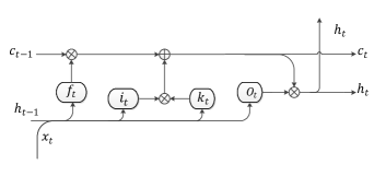
Figure 1: LSTM block at time $t$

4 DL-based Spatio-Temporal Forecasting (DL-STF)

In this section, we outline our proposed spatio-temporal forecasting scheme which is based on DL. We namely call our algorithm DL-based Spatio-Temporal Forecasting (DL-STF). Let graph $G$ be defined as $G\triangleq[E,V]$ where $E$ denotes the edges and $V=\{v_{1},\dots,v_{n}\}$ denotes the nodes. Each node of the graph $v_{i}$ generates data at each time step. Node $v_{i}$ at time $t$ generates $x^{t}_{i}$ which is a scalar (e.g., wind speed in our problem). Assume $x^{t}_{i}$ is sampled from an unknown distribution $P_{real}(x)$. Also $s^{t}=[x^{t}_{1},x^{t}_{2}\dots x^{t}_{n}]$ (it is a vector) contains the output of all nodes at time $t$.Similarly, let $\hat{x}^{t}_{i}$ be the output prediction of node $i$ at time $t$. Let $\hat{s}^{t}=[\hat{x}^{t}_{1},\hat{x}^{t}_{2}\dots\hat{x}^{t}_{n}]$ be the vector containing prediction of all nodes (same size as $s^{t}$). We assume we only have real data for all nodes every $h$ time steps. Our goal is to predict $s^{t}$, using {$s^{k}\},k\in\{t-\ell,t-\ell+1,...,t-1\}$. Based on moving horizon scheme, when real value for $s^{k}$ is not available, we use its prediction, $\hat{s}^{k}$.

4.1 Time step models

We have access to real data every $h$ hours and want to forecast wind speed for the next $h$ hours. In different time steps we have different kind of inputs. For the first time step, we have real data for all inputs but for the next time step, we have real data for all inputs except one. For that one we use forecast data from previous step. This scheme repeats for all the $h$ steps. Based on this paradigm, we define a specific model for each time step over the input horizon. In order to train the model, we use real values as much as we can, but if we do not have real values, we use forecast values from previous trained models. So for example the model for forecasting at time $t+2$ should differ from model for forecasting at time $t+3$. If we have $n$ stations, the input for our algorithm is an $n$-dimensional vector at each time step and we forecast an $n$-dimensional vector for next time step.

Let $t$ denote the global time index, $h$ the number of time steps in moving horizon, and $\ell$ the input horizon. We train $h$ different models. Model number $i$ is represented by $M_{i}$. We define $\hat{t}=t~{}\text{mod}~{}h$ and the relation between $\hat{t}$ and $i$ is as follows:

$$i=\begin{cases}\hat{t}&,\text{if}~{}\hat{t}\neq 0\\ h&,\text{if}~{}\hat{t}=0\end{cases}$$ (2)

The input and output of each model is different from others. Also structure, number of parameters, and details of each model could be different from others. This flexibility in defining and customizing the models based on the time step during the prediction horizon ($h$) is one of the strength of our framework. For $i=1,2,\cdots,h$, we have:

• Model: $M_{i}$

• Input: $\{s^{t-\ell},s^{t-\ell+1},...,~{}s^{t-i},\hat{s}^{t-i+1},...,\hat{s}^{t-1}\}$

  ($\ell-i+1$ real values, $i-1$ forecasted values)

• Algorithm: RNN with LSTM blocks

• Output: Forecast of output of all nodes, $\hat{s}^{t}$

$\hat{s}^{t}$ is output of the model $M_{i}$, which $i$ is calculated from (2). If $t-l$ is greater than $t-i$ then we only use the last $l$ predicted values. Also if $t-i+1$ is equal to $t$, only real values are used. Loss function for each model $M_{i}$ is defined as $L(M_{i}(\{s^{t-\ell},...~{}s^{t-i},\hat{s}^{t-i+1},...~{}\hat{s}^{t-1}\}),x^{t})$ where $x^{t}$ is the real output of the nodes in the graph at time $t$ and $L(a,b)$ is the mean absolute error of $a$ and $b$. In figure 2 we show the overview of the model’s detail.

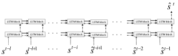
Figure 2: The model $M_{i}$ trained at time t. Inputs are $s^{t-\ell},s^{t-\ell+1},...,~{}s^{t-i}$ (real values) and $\hat{s}^{t-i+1},...~{}\hat{s}^{t-1}$ (forecasted values from previous trained models). Black thick and dashed arrows are $c_{t}$ and $h_{t}$ based on Figure 1.

5 Case Study of 57 Stations in East Coast

We apply DL-STF to real wind speed data. East coast states are good candidates for our study as: (i) wind speed profiles are higher and (ii) there are more stations in a close vicinity in these states.

5.1 Data Description

We use hourly wind speed data from Meteorological Terminal Aviation Routine (METAR) weather reports of 57 stations in east coast including Massachusetts, Connecticut, New York, and New Hampshire (Iowa Environmental Mesonet, 2014). Fig. 3 depicts the area under study and the location of these 57 stations. The target station  Nantucket Memorial Airport (ACK) (circled in red) is located on an island and is subject to wind profiles with high ramps and speeds due to the fact that the surrounding surface has very low roughness heights. Furthermore, this area has good correlations with other stations owing to the fact the prevailing wind direction of this region is mainly northwest or southeast.

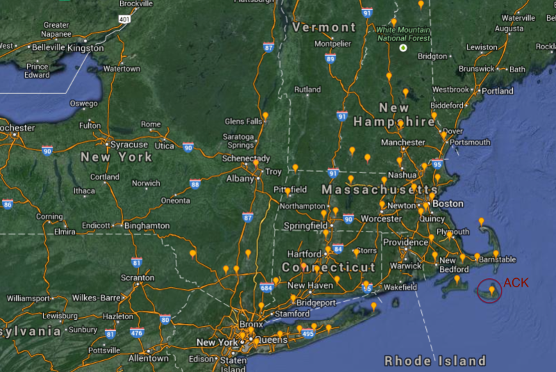
Figure 3: Map of the area under study. The $57$ measuring locations in east coast are shown with yellow points. Circled in red is the target station ACK.

A time period from January 6, 2014 to February 20, 2014 is considered as test set in our simulations. This time period has the most unsteady wind conditions throughout the year.

5.2 Results and Discussion

In this section we discuss the details about our implementation and hyper-parameters setting. In our experiments $h=6$ and we chose $\ell=12$ based on a cross validation study. The optimizer is MSRProp which shows good performance for RNN with learning rate of $0.001$. The activation function is ReLu. Data is normalized between 0 and 1. We use one fully connected layer on top of $h_{t}$ features to create the desired output layer.

We use TensorFlow (Abadi & et al., 2015) and Keras (Chollet et al., 2015) and our code and data are available online. For models whose input includes predicted values, we need to increase the model capacity to help overcome over-fitting. Thus, we increase the number of neurons and layers and use stacked LSTM. To show performance of our algorithm we use three common error measure MAE, RMSE, and NRMSE. Table 1 shows comparison of three common error measures between proposed method and other methods. It is worth mentioning that other existing methods are trained to forecast only one node at a time but our method can forecast the output of all nodes in the graph at one time. More importantly, as we can see the error comparisons, our method has smaller error values compared to all other methods and outperform state-of-the-art results. More details about how other methods work are available in (Sanandaji et al., 2015), (Tascikaraoglu et al., 2016).

Table 1: Error measures for different methods for one node (ACK)

Method	MAE	RMSE	NRMSE
	(m/s)	(m/s)	(%)
Persistence Forecasting	2.14	2.83	16.86
AR of order 1	2.07	2.76	16.44
AR of order 3	2.07	2.76	16.40
WT-ANN	1.82	2.47	14.68
AN-based ST	1.80	2.30	13.69
LS-based ST	1.72	2.20	13.08
DL-STF	1.63	2.19	13.08
DL-STF(All nodes)	1.18	1.62	16.28

Table 2 shows the average of three error measures for all nodes in the graph. To the best of our knowledge there is no other method capable of forecasting outputs of all nodes in a graph in one framework. The average of the error measures of all nodes is even better than error measures for one node(ACK) with relative improvement about 27% for MAE and RMSE.

Table 2: Average error measures over all locations using DL-STF

	MAE(m/s)	RMSE(m/s)	NRMSE(%)
Our method	1.18	1.62	16.28

In DL-STF, we model all information and the hidden interactions between nodes of the graph. As explained earlier, in a spatio-temporal setting we use information of all nodes to forecast one node’s output in order to improve the forecasting performance as compared to the case when we only use one node’s data (temporal setting). Table 3 illustrates a comparison between these two cases: 1) DL-STF trained on all nodes of the graph to forecast one node’s output (node ACK) and 2) DL-STF trained with data only from node ACK and, thus, we don’t count for hidden relationships between nodes. Table 3 shows that the error measures in case 1 (spatio-temporal forecasting) has significantly improved.

Table 3: Comparison of forecasting error measures. First row: train only on data from the node ACK and test on the node ACK. Second row: train on data from all nodes of the graph and test on the node ACK. Third row: train on data from all nodes and test on all nodes and calculate the average error measures over all nodes.

	MAE(m/s)	RMSE(m/s)	NRMSE(%)
one node	1.99	2.60	15.46
all nodes (ACK)	1.63	2.19	13.08
mean all nodes	1.18	1.62	16.28

In Figure 4 we show the accuracy of forecasting for 16 nodes of the graph. It shows real values vs forecast values on test data. The average of error measures are 1.203, 1.663, 16.378 for MAE, RMSE, NRMSE respectively.

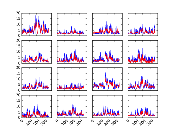
Figure 4: Forecasting performance on 16 stations. Blue lines are real values and red ones are forecast values. Horizontal axis shows time steps and vertical axis shows wind speed(m/s).

6 Conclusion

A spatio-temporal wind speed forecasting algorithm using DL is presented. In our proposed framework, we model the spatio-temporal information by a graph whose nodes are data generating entities and its edges basically model how these nodes are interacting with each other. One of the main contributions of our work is the fact that we obtain forecasts of all nodes of the graph at the same time. Results of a case study on recorded time series data from a collection of wind mills in the north-east of the U.S. show that the proposed DL-based forecasting algorithm significantly improves the short-term forecasts compared to a set of widely-used benchmarks models.

References

- Abadi & et al. (2015) Abadi, Martín and et al. TensorFlow: Large-scale machine learning on heterogeneous systems, 2015. URL http://tensorflow.org/. Software available from tensorflow.org.
- CEC (2013) CEC, (California Energy Commission). California renewable energy overview and programs. 2013. URL http://www.energy.ca.gov/renewables/index.html.
- Chollet et al. (2015) Chollet, François et al. Keras. https://github.com/fchollet/keras, 2015.
- Deng et al. (2009) Deng, Jia, Dong, Wei, Socher, Richard, Li, Li-Jia, Li, Kai, and Fei-Fei, Li. Imagenet: A large-scale hierarchical image database. In Computer Vision and Pattern Recognition, 2009. CVPR 2009. IEEE Conference on, pp. 248–255. IEEE, 2009.
- Dowell et al. (2013) Dowell, Jethro, Weiss, Stephan, Hill, David, and Infield, David. Short-term spatio-temporal prediction of wind speed and direction. Wind Energy, 2013.
- Gneiting et al. (2006) Gneiting, Tilmann, Larson, Kristin, Westrick, Kenneth, Genton, Marc G., and Aldrich, Eric. Calibrated probabilistic forecasting at the stateline wind energy center: The regime-switching space–time method. Journal of the American Statistical Association, 101(475):968–979, 2006.
- Goodfellow et al. (2016) Goodfellow, Ian, Bengio, Yoshua, and Courville, Aaron. Deep learning, 2016.
- Graves (2013) Graves, Alex. Generating sequences with recurrent neural networks. arXiv preprint arXiv:1308.0850, 2013.
- Grover et al. (2015) Grover, Aditya, Kapoor, Ashish, and Horvitz, Eric. A deep hybrid model for weather forecasting. In Proceedings of the 21th ACM SIGKDD International Conference on Knowledge Discovery and Data Mining, pp. 379–386. ACM, 2015.
- Hao et al. (2013) Hao, He, Sanandaji, Borhan M., Poolla, Kameshwar, and Vincent, Tyrone L. Aggregate flexibility of thermostatically controlled loads. IEEE Transactions on Power Systems, 2013.
- He et al. (2014) He, Miao, Yang, Lei, Zhang, Junshan, and Vittal, Vijay. A spatio-temporal analysis approach for short-term forecast of wind farm generation. IEEE Transactions on Power Systems, 29(4):1611–1622, 2014.
- Hering & Genton (2010) Hering, Amanda S and Genton, Marc G. Powering up with space-time wind forecasting. Journal of the American Statistical Association, 105(489):92–104, 2010.
- Hochreiter & Schmidhuber (1997) Hochreiter, Sepp and Schmidhuber, Jürgen. Long short-term memory. Neural computation, 9(8):1735–1780, 1997.
- IEA (2013) IEA, (International Energy Agency). Technology roadmap: Wind energy. 2013. URL http://www.iea.org/publications/freepublications/publication/Wind_2013_Roadmap.pdf.
- Iowa Environmental Mesonet (2014) Iowa Environmental Mesonet. ASOS historical data, 2014. URL http://mesonet.agron.iastate.edu/ASOS/.
- Krizhevsky et al. (2012) Krizhevsky, Alex, Sutskever, Ilya, and Hinton, Geoffrey E. Imagenet classification with deep convolutional neural networks. In Advances in neural information processing systems, pp. 1097–1105, 2012.
- Li & Shi (2010) Li, Gong and Shi, Jing. On comparing three artificial neural networks for wind speed forecasting. Applied Energy, 87(7):2313–2320, 2010.
- Ma et al. (2017) Ma, Xuejiao, Jin, Yu, and Dong, Qingli. A generalized dynamic fuzzy neural network based on singular spectrum analysis optimized by brain storm optimization for short-term wind speed forecasting. Applied Soft Computing, 54:296–312, 2017.
- Ren et al. (2015) Ren, Shaoqing, He, Kaiming, Girshick, Ross, and Sun, Jian. Faster r-cnn: Towards real-time object detection with region proposal networks. In Conference on Neural Information Processing Systems (NIPS 2015), 2015.
- Sanandaji et al. (2014) Sanandaji, Borhan M., Hao, He, Poolla, Kameshwar, and Vincent, Tyrone L. Improved battery models of an aggregation of thermostatically controlled loads for frequency regulation. In American Control Conference (ACC 2014), 2014.
- Sanandaji et al. (2015) Sanandaji, Borhan M, Tascikaraoglu, Akin, Poolla, Kameshwar, and Varaiya, Pravin. Low-dimensional models in spatio-temporal wind speed forecasting. In American Control Conference (ACC 2015), pages 4485–4490. arXiv preprint arXiv:1503.01210, 2015.
- Smith et al. (2007) Smith, J. Charles, Milligan, Michael R., DeMeo, Edgar A., and Parsons, Brian. Utility wind integration and operating impact state of the art. IEEE Transactions on Power Systems, 22(3):900–908, 2007.
- Sutskever et al. (2014) Sutskever, Ilya, Vinyals, Oriol, and Le, Quoc V. Sequence to sequence learning with neural networks. In Advances in neural information processing systems, pp. 3104–3112, 2014.
- Tascikaraoglu & Uzunoglu (2014) Tascikaraoglu, A and Uzunoglu, M. A review of combined approaches for prediction of short-term wind speed and power. Renewable and Sustainable Energy Reviews, 34:243–254, 2014.
- Tascikaraoglu et al. (2016) Tascikaraoglu, Akin, Sanandaji, Borhan M, Poolla, Kameshwar, and Varaiya, Pravin. Exploiting sparsity of interconnections in spatio-temporal wind speed forecasting using wavelet transform. Applied Energy, 165:735–747, 2016.
- Tastu et al. (2011) Tastu, Julija, Pinson, Pierre, Kotwa, Ewelina, Madsen, Henrik, and Nielsen, Henrik Aa. Spatio-temporal analysis and modeling of short-term wind power forecast errors. Wind Energy, 14(1):43–60, 2011.
- Tastu et al. (2014) Tastu, Julija, Pinson, Pierre, Trombe, P-J, and Madsen, Henrik. Probabilistic forecasts of wind power generation accounting for geographically dispersed information. IEEE Transactions on Smart Grid, 5(1):480–489, 2014.
- Wang et al. (2016) Wang, HZ, Wang, GB, Li, GQ, Peng, JC, and Liu, YT. Deep belief network based deterministic and probabilistic wind speed forecasting approach. Applied Energy, 182:80–93, 2016.
- Wytock & Kolter (2013) Wytock, Matt and Kolter, Zico. Large-scale probabilistic forecasting in energy systems using sparse gaussian conditional random fields. Proceedings of the nd IEEE Conference on Decision and Control, pp. 1019–1024, 2013.
- Xie et al. (2014) Xie, Le, Gu, Y., Zhu, X., and Genton, M. G. Short-term spatio-temporal wind power forecast in robust look-ahead power system dispatch. IEEE Transactions on Smart Grid, 5(1):511–520, 2014.
- Zhang et al. (2014) Zhang, Yao, Wang, Jianxue, and Wang, Xifan. Review on probabilistic forecasting of wind power generation. Renewable and Sustainable Energy Reviews, 32:255–270, 2014.
- Zhu & Genton (2012) Zhu, Xinxin and Genton, Marc G. Short-term wind speed forecasting for power system operations. International Statistical Review, 80(1):2–23, 2012.