Global Finite-Time Attitude Consensus of Leader-Following Spacecraft Systems Based on Distributed Observers

Abstract

This paper addresses the leader-following attitude consensus problem for a group of spacecraft when at least one follower can access the leader’s attitude and velocity relative to the inertial space. A nonlinear distributed observer is designed to estimate the leader’s states for each follower. The observer possesses one important and novel feature of keeping attitude and angular velocity estimation errors on second-order sliding modes, and thus provides finite-time convergent estimates for each follower. Further, quaternion-based hybrid homogeneous controllers recently developed for single spacecraft are extended and then applied, by establishing a separation principle with the proposed observer, to track the leader’s attitude motion. As a result, global finite-time attitude consensus is achieved on the entire attitude manifold, with either full-state measurements or attitude-only measurements, as long as the network topology among the followers is undirected and connected. Numerical simulations are presented to demonstrate the performance of the proposed methods.

I Introduction

Distributed attitude consensus of multiple cooperative spacecraft has drawn increasing attention due to its applications in formation flying, space-based interferometry, in-orbit assembly, etc. It can be classified as two types, namely, leaderless consensus that requires all spacecraft to reach an arbitrary yet probably a priori unknown synchronized state [1], and leader-following consensus that requires each follower to track a prescribed group attitude trajectory provided by a real or virtual leader [2, 3, 4]. This paper mainly focuses on the leader-following type.

The leader-following attitude consensus issue was first addressed by assuming that the leader’s trajectory is available to all followers [2, 3, 4, 5, 6]. In practice, a more common yet challenging case is that only a portion of the followers can access the state of the leader. To deal with this problem, first-order sliding mode estimators were derived in [7, 8] and [9] to estimate the reference attitude and/or velocity in finite time. These designs can be traced back to the work of [10] for single/double-integrator systems. Asymptotic distributed estimators were also proposed when the reference angular velocity is linearly parameterized [11] or generated by a known, stable, linear system [12, 13]. The methods of [14, 6] and [15] involve no estimators but require the spacecraft to transmit their accelerations apart from their attitudes and velocities. Among the above methods, those of [15] and [9], further guarantee finite-time stability, which implies that the consensus behavior can be achieved in finite time instead of infinite time as for asymptotic or exponential stability. In addition, angular velocity measurements are not needed for the consensus algorithms of [16, 3, 6, 8, 9] and [13].

Another important issue is the complex nonlinearity intrinsic in attitude control. More precisely, the attitude configuration, the set of $3\times 3$ rotation matrices SO(3), is a nonlinear manifold not diffeomorphic to any Euclidean space and precludes the existence of continuous, globally stabilizing, state-feedback laws on SO(3) [17, 18]. In addition, the attitude kinematics and dynamics are both nonlinear. Due to these features, the attitude consensus laws extended from algorithms for linear systems ensure merely local or at most almost global stability [19, 1] while the methods of [8] and [9] result in semi-global stability. In addition, some quaternion-based control schemes can cause the undesirable unwinding phenomenon due to neglecting that the unit-quaternion space is a double-covering of SO(3) [14, 11, 12, 13]. To overcome this problem, [5] developed a hybrid feedback scheme with network-based hysteretic switching logics, resulting in global attitude consensus and simultaneous robustness to measurement noise. This method, however, relies on the availability of the leader’s state to all followers and, similarly to [3] and [11], does not allow cycles in the communication graph. Otherwise, undesirable equilibria other than the consensus state can arise and fail the control objective.

This paper investigates the global attitude consensus of a leader-following spacecraft network in terms of the quaternion parameterization. The communication graph between followers is assumed to be an undirected connected graph and only a subset of the followers has access to the dynamic leader. In order to estimate the leader’s states for each follower, a novel nonlinear distributed observer is designed such that finite-time convergence is guaranteed only if at least one follower connects to the leader. Following this, the hybrid homogeneous attitude controllers developed in [20] are extended and then applied together with the distributed observer to perform consensus control by establishing a separation principle [21]. More precisely, the resultant consensus laws can restore the uniformly globally finite-time stable systems of [20], in both the full-state measurement case and attitude-only measurement case, where the latter relies on a quaternion filter to inject the necessary damping instead of velocity feedback. As a result, the proposed control schemes avoid the unwinding problem and achieve global finite-time attitude consensus which, to the best of the our knowledge, has not been reported in existing cooperative attitude control literature. As another contribution, the proposed observer requires only the boundedness of the leader’s angular velocity and its derivatives for finite-time convergence and hence possesses better robustness and allows more generic reference trajectories than the distributed observers in [12, 13] which are limited to stationary or periodic reference trajectories. In addition, it keeps the attitude and angular velocity estimation errors on second-order sliding modes, indicating higher accuracy during digital implementation than the distributed estimator derived in [10] and its variants in [7, 8] and [9] that all attain first-order sliding modes.

The remainder of this paper is organized as follows. Basic notations, system equations and graph theory are reviewed in Section II. A nonlinear distributed observer with finite-time convergence is designed to estimate the leader’s states in Section III. With the estimates from the observer, controller laws are derived in Section IV based on the results of [20] to attain global attitude consensus of the entire leader-following spacecraft system under two measurement scenarios. Section V presents numerical examples to illustrate the effectiveness of the proposed methods and Section VI draws the conclusions.

II Preliminaries

Throughout this paper, denote by $I_{n}$ the $n\times n$ identity matrix, $\mathbf{1}_{n}=[1,...,1]^{T}$, and $\mathbb{I}_{n}=\{1,...,n\}$. For all $x\in{\mathbb{R}}$ and $\alpha\geq 0$, let $\textup{sgn}^{\alpha}(x)=\textup{sgn}(x)|x|^{\alpha}$ and $\textup{sat}_{\alpha}(x)=\textup{sgn}(x)\textup{min}\{|x|^{\alpha},1\}$, where $\textup{sgn}(\cdot)$ is the standard sign function. Clearly, $\textup{sgn}^{\alpha}(x)$ is a continuous nonsmooth function if $0<\alpha<1$, while $\textup{sat}_{\alpha}(x)$ becomes the standard saturation function $\textup{sat}(x)$ if $\alpha=1$. For all $x=[x_{1},\cdots,x_{n}]^{T}\in{\mathbb{R}^{n}}$ and $\alpha\geq 0$, let $\textup{sgn}^{\alpha}(x)=[\textup{sgn}^{\alpha}(x_{1}),...,\textup{sgn}^{\alpha}(x_{n})]$ and $\textup{sat}_{\alpha}(x)=[\textup{sat}_{\alpha}(x_{1}),...,\textup{sat}_{\alpha}(x_{n})]$. Denote by $\|{\cdot}\|_{p}$ the $p$-norm of a vector respectively for $p=1,2,\infty$. For all $A\in\mathbb{R}^{m\times n}$, let $\bar{\sigma}(A)$ and $\underline{\sigma}(A)$ be its maximum and minimum singular values respectively. Note that $\bar{\sigma}(A)$ equals to its induced 2-norm $\|A\|_{2}=\textup{max}_{\{x\in\mathbb{R}^{n}:\|x\|_{2}=1\}}\|Ax\|_{2}$. Given $x\in{\mathbb{R}^{3}}$, $x^{\times}$ is the skew-symmetric matrix satisfying $x^{\times}y=x\times y$, $\forall y\in{\mathbb{R}^{3}}$, where $\times$ is the cross product on $\mathbb{R}^{3}$.

A quaternion $Q=[\eta,q^{T}]^{T}\in{\mathbb{R}^{4}}$ consists of a scalar part $\eta\in{\mathbb{R}}$ and a vector part $q\in\mathbb{R}^{3}$. Let $\textup{vec}(Q)$ give the vector part of $Q$, i.e., $\textup{vec}(Q)=q$. The quaternion multiplication is defined as

$$Q\circ Q^{\prime}=\left[\begin{array}[]{c}\eta{\eta^{\prime}}-q^{T}q^{\prime}\\ \eta q^{\prime}+\eta^{\prime}q+q\times q^{\prime}\end{array}\right],Q^{\prime}=[\eta^{\prime},q^{\prime T}]^{T}\in{\mathbb{R}^{4}}$$

which is associative and distributive but is not commutative. In addition, the conjugation of $Q$ is given by $Q^{*}=[\eta,-q^{T}]^{T}\in{\mathbb{R}^{4}}$. Note that $(Q\circ Q^{\prime})^{*}=(Q^{\prime})^{*}\circ Q^{*}$. A 3-D vector is treated as a quaternion with zero scalar part when operating with a quaternion. With the identity element $\textbf{1}=[1,0,0,0]^{T}$, the set of unit quaternions is defined as $\mathbb{S}^{3}=\{Q\in{\mathbb{R}^{4}}:Q\circ Q^{*}=\textbf{1}\}$.

II-A System Equations

Consider a system of n rigid spacecraft (agents). Denote by $Q_{i}=[\eta_{i},q_{i}^{T}]^{T}\in{\mathbb{S}^{3}}$, $\forall i\in\mathbb{I}_{n}$, the attitude quaternion of the body-fixed frame of the ith agent, $\mathcal{F}_{i}$, relative to the inertial frame $\mathcal{F}_{I}$. The equations of motion of the ith agent are

$$\dot{Q}_{i}={1\over 2}Q_{i}\circ{\omega_{i}}={1\over 2}E(Q_{i})\omega_{i},\;E(Q_{i})=\begin{bmatrix}-q_{i}^{T}\\ q_{i}^{\times}+\eta_{i}I_{3}\end{bmatrix}$$ (1)

$$J_{i}\dot{\omega}_{i}=-\omega_{i}\times{J_{i}\omega_{i}}+u_{i},$$ (2)

where $\omega_{i}\in{\mathbb{R}^{3}}$ and $J_{i}=J_{i}^{T}$ are the angular velocity and inertia tensor of agent i expressed in $\mathcal{F}_{i}$. $u_{i}$ is the corresponding control torque. The rotation matrix from $\mathcal{F}_{I}$ to $\mathcal{F}_{i}$ can be computed from $Q_{i}$ by

$$R(Q_{i})=(\eta_{i}^{2}-q_{i}^{T}q_{i})I_{3}-2\eta_{i}q_{i}^{\times}+2q_{i}q_{i}^{T}.$$ (3)

Assume that the desired trajectory is generated by a leader spacecraft with body-fixed frame $\mathcal{F}_{0}$. Denote by $Q_{0}\in{\mathbb{S}^{3}}$ and $\omega_{0}\in{\mathbb{R}^{3}}$ the attitude quaternion and angular velocity of $\mathcal{F}_{0}$ relative to $\mathcal{F}_{I}$. In addition, $(Q_{0},\omega_{0})$ obeys the same kinematics as (1). The attitude and angular velocity error of the ith follower relative to the leader is defined as $Q_{i0}=Q_{0}^{*}\circ Q_{i}$ and $\omega_{i0}=\omega_{i}-R(Q_{i0})\omega_{0}$. Letting $\bar{\omega}_{i0}=R(Q_{i0})\omega_{0}$, the system equations in terms of $Q_{i0}$ and $\omega_{i0}$ are then written as

$$\dot{Q}_{i0}={1\over 2}Q_{i0}\circ{\omega_{i0}}={1\over 2}E(Q_{i0})\omega_{i0},$$ (4)

$$J_{i}\dot{\omega}_{i0}=\Xi(\omega_{i0},\bar{\omega}_{i0})\omega_{i0}-u_{fi}+u_{i},$$ (5)

where $\Xi(\omega_{i0},\bar{\omega}_{i0})=(J_{i}\omega_{i0}+J_{i}\bar{\omega}_{i0})^{\times}-\bar{\omega}_{i0}^{\times}J_{i}-J_{i}\bar{\omega}_{i0}^{\times}$ is skew-symmetric and

$$u_{fi}=J_{i}R(Q_{i0})\dot{\omega}_{0}+\bar{\omega}_{i0}^{\times}J_{i}\bar{\omega}_{i0},$$ (6)

represents the torque to be compensated for perfect tracking of the desired trajectory. When every follower has access to the leader’s trajectory, attitude consensus can be achieved by applying the controllers of [22] and [20] to globally stabilize $(Q_{i0},\omega_{i0})=(\pm\textbf{1},0)$, $i\in{\mathbb{I}_{n}}$. These methods, however, cannot be applied if the leader’s trajectory is available to only one or some of the followers.

As many studies on coordinated attitude control of formation flying spacecraft, the above dynamics models assume that all spacecraft share the same inertial frame $\mathcal{F}_{I}$. This is true in practice because the the inertial frame is usually set as the Earth-centered inertial frame for Earth spacecraft systems, and the heliocentric inertial frame for deep-space spacecraft systems.

II-B Communication Graph

The information flow for n followers is assumed to be bidirectional and can be described by a weighted undirected graph $\mathcal{G}\triangleq(\mathcal{V},\mathcal{E})$, where $\mathcal{V}=\{1,...,n\}$ is the node set and $\mathcal{E}\subseteq{\mathcal{V}\times\mathcal{V}}$ is the edge set. Since $\mathcal{G}$ is undirected, it follows that $(j,i)\in{\mathcal{E}}\Leftrightarrow(i,j)\in{\mathcal{E}}$, which means that there exists an edge between agents i and j. The adjacency matrix $A=[a_{ij}]_{n\times n}\in\mathbb{R}^{n\times n}$ is defined such that $a_{ij}=a_{ji}>0$ if $(j,i)\in{\mathcal{E}}$ while $a_{ij}=0$ otherwise. In addition, we set $a_{ii}=0$, $\forall i\in\mathcal{V}$. Denote by $L=[l_{ij}]_{n\times n}\in\mathbb{R}^{n\times n}$ the Laplacian matrix of $\mathcal{G}$ with $l_{ii}=\sum_{j=1}^{n}a_{ij}$ and $l_{ij}=-a_{ij}$ for $i\neq j$. Label the leader as node 0 and denote by $\bar{\mathcal{G}}$ the leader-following graph. Let $a_{i0}\geq 0$ be the connection weight between the leader and follower i such that $a_{i0}=1$ if follower i connects to the leader and otherwise $a_{i0}=0$. Denote by $A_{0}=\textup{diag}\{a_{10},...,a_{n0}\}$. $\mathcal{G}$ is said to be connected if there is path between any two agents. Additionally, let $\bar{\mathcal{G}}\triangleq(\bar{\mathcal{V}},\bar{\mathcal{E}})$ represent the leader-following graph, where $\bar{\mathcal{V}}=\{0\}\cup{\mathcal{V}}$ and $\bar{\mathcal{E}}\subseteq{\bar{\mathcal{V}}\times\bar{\mathcal{V}}}$. In order for the development of distributed attitude consensus schemes, the following assumptions and lemmas are introduced.

Assumption II.1

The communication among the followers is constant and bidirectional and the leader-following graph $\bar{\mathcal{G}}$ contains a spanning tree rooted at node 0, i.e., there is a path from the leader to any follower.

Assumption II.2

The leader’s angular velocity $\omega_{0}(t)$ and its first two derivatives are continuous in time, and there exist constants $\gamma_{i}$, $i\in{\mathbb{I}_{3}}$, such that $\|\omega_{0}(t)\|_{\infty}\leq{\gamma_{1}}$, $\|\dot{\omega}_{0}(t)\|_{\infty}\leq{\gamma_{2}}$, and $\|\ddot{\omega}_{0}(t)\|_{\infty}\leq{\gamma_{3}}$.

Lemma II.1

[23] If Assumption II.1 holds, then $H\triangleq L+A_{0}$ is positive definite.

Lemma II.2

[24] Consider the system $\dot{x}=-\rho_{1}\text{sgn}^{\frac{1}{2}}(x)+y$, $\dot{y}=-\rho_{2}\text{sgn}(x)+f(t)$ with $|f(t)|\leq f_{0}$, where $f_{0}$, $\rho_{1}$, and $\rho_{2}$ are constants. If $\rho_{1}>0$ and $\rho_{2}>f_{0}$, then $x(t)$ and $y(t)$ converge to zero in a finite time $t_{r}\geq 0$, which can be estimated by the algorithm given in [24].

Lemma II.3

[25] If $0<\alpha\leq 1$, then $(\sum_{i=1}^{n}|x_{i}|)^{\alpha}\leq\sum_{i=1}^{n}|x_{i}|^{\alpha}\leq n^{1-\alpha}(\sum_{i=1}^{n}|x_{i}|)^{\alpha}$ holds, $\forall x_{i}\in\mathbb{R}^{n}$ and $\forall i\in\mathbb{I}_{n}$.

The matrix $E(\cdot)$ defined in (1) has the following useful properties and their proofs are given in Appendix A:

Lemma II.4

For any $Q,Q^{\prime}\in{\mathbb{R}^{4}}$, we have $\|E(Q)\|_{2}=\|Q\|_{2}$, ${Q^{T}}E(Q^{\prime})=-\textup{vec}^{T}(Q^{*}\circ{Q^{\prime}})$, and ${Q^{T}}E(Q)=0$.

Lemma II.5

For any $Q_{i}\in{\mathbb{R}^{4}}$, $b_{ij}\in{\mathbb{R}}$ and $b_{ij}=b_{ji}$, $i,j\in{\mathbb{I}_{n}}$ we have $\sum_{i=1}^{n}\sum_{j=1}^{n}b_{ij}{Q_{j}^{T}}E(Q_{i})=0.$

As shown in the next section, Lemmas II.4 and II.5 are useful for proving the stability of the proposed distributed observers.

III Distributed Finite-Time Observer Design

In this section, a distributed observer is derived to obtain the leader’s trajectory $(Q_{0},\omega_{0},\dot{\omega}_{0})$ for each agent in finite time when only a subset of the followers can access the leader’s attitude and angular velocity relative to the inertial space.

Denote by $(P_{i},v_{i},z_{i})\in\mathbb{R}^{4}\times\mathbb{R}^{3}\times\mathbb{R}^{3}$ the estimate of $(Q_{0},\omega_{0},\dot{\omega}_{0})$ by the ith follower. Letting $(P_{0},v_{0},z_{0})=(Q_{0},\omega_{0},\dot{\omega}_{0})$, a nonlinear distributed observer is then designed as

$$\dot{P}_{i}=\frac{1}{2}P_{i}\circ v_{i}-\lambda_{1}\textup{sgn}^{\beta_{1}}\left(\sum_{j=0}^{n}a_{ij}(P_{i}-P_{j})\right),$$ (7)

$$\dot{v}_{i}=z_{i}-\lambda_{2}\textup{sgn}^{\beta_{2}}\left(\sum_{j=0}^{n}a_{ij}(v_{i}-v_{j})\right),$$ (8)

$$\dot{z}_{i}=-\lambda_{3}\textup{sgn}\left(a_{i0}(z_{i}-w_{i})+\sum_{j=1}^{n}a_{ij}(z_{i}-z_{j})\right),$$ (9)

where $(P_{i}(0),v_{i}(0),z_{i}(0))\in\mathbb{R}^{4}\times\mathbb{R}^{3}\times\mathbb{R}^{3}$, $i\in{\mathbb{I}_{n}}$, $\lambda_{1},\lambda_{2}>0$, $0<\beta_{1},\beta_{2}<1$, and $\lambda_{3}>\gamma_{3}$. Since the leader’s acceleration $\dot{\omega}_{0}$ is not available for any follower, it is recovered from the velocity $\omega_{0}$ via the second-order sliding mode differentiator

$$\left\{\begin{array}[]{cll}\dot{y}_{i}&=&-\mu_{1}a_{i0}\text{sgn}^{\frac{1}{2}}(y_{i}-\omega_{0})+w_{i}\\ \dot{w}_{i}&=&-\mu_{2}a_{i0}\text{sgn}(y_{i}-\omega_{0})\end{array}\right.,$$ (10)

where $y_{i}(0)=w_{i}(0)=0$, $\mu_{1}>0$ and $\mu_{2}\geq\gamma_{3}$. Note that the right-hand sides of $\dot{P}_{i}$, $\dot{v}_{i}$, and $\dot{y}_{i}$ are continuous while those of $\dot{z}_{i}$ and $\dot{w}_{i}$ are discontinuous and their solutions are understood in the Filippov sense [26].

Next, we define the following estimation errors

$$\begin{array}[]{c}\tilde{P}_{i}=P_{i}-P_{0},\,\tilde{v}_{i}=v_{i}-v_{0},\,\tilde{z}_{i}=z_{i}-z_{0},\\ \tilde{y}_{i}=y_{i}-\omega_{0},\,\tilde{w}_{i}=w_{i}-\dot{\omega}_{0},\,i\in{\mathbb{I}_{n}}.\end{array}$$ (11)

In addition, denote by

$$x_{si}=\sum_{j=0}^{n}a_{ij}(x_{i}-x_{j})=a_{i0}\tilde{x}_{i}+\sum_{j=1}^{n}a_{ij}(\tilde{x}_{i}-\tilde{x}_{j}),\\ x\in\{P,v,z\},\,i\in{\mathbb{I}_{n}}.$$ (12)

For convenience, introduce the aggregate variables

$$\tilde{x}=[\tilde{x}_{1}^{T},\cdots,\tilde{x}_{n}^{T}]^{T},\,x_{s}=[x_{s1}^{T},\cdots,x_{sn}^{T}]^{T},\,x\in\{P,v,z\},$$

which satisfy

$$P_{s}=(H\otimes I_{4})\tilde{P},\,v_{s}=(H\otimes I_{3})\tilde{v},\,z_{s}=(H\otimes I_{3})\tilde{z},$$ (13)

where $\otimes$ is the Kronecker product. Differentiating the expressions in (11) and applying (7)-(10), the equations of the estimation errors can then be written as

$$\dot{\tilde{P}}_{i}=0.5(P_{i}\circ v_{i}-P_{0}\circ v_{0})-\lambda_{1}\textup{sgn}^{\beta_{1}}(P_{si}),\,i\in{\mathbb{I}_{n}},$$ (14)

$$\dot{\tilde{v}}=\tilde{z}-\lambda_{2}\textup{sgn}^{\beta_{2}}(v_{s}),$$ (15)

$$\dot{\tilde{z}}=-\lambda_{3}\textup{sgn}(z_{s}-A_{0}\tilde{w})-\textbf{1}_{n}\otimes{\dot{z}_{0}}.$$ (16)

$$\left\{\begin{array}[]{cll}\dot{\tilde{y}}_{i}&=&-\mu_{1}a_{i0}\text{sgn}^{\frac{1}{2}}(\tilde{y}_{i})+\tilde{w}_{i}\\ \dot{\tilde{w}}_{i}&=&-\mu_{2}a_{i0}\text{sgn}(\tilde{y}_{i})-\ddot{\omega}_{0}\end{array}\right.,\,i\in{\mathbb{I}_{n}},$$ (17)

where $\tilde{w}=[\tilde{w}_{1}^{T},\cdots,\tilde{w}_{n}^{T}]^{T}\in\mathbb{R}^{3n}$.

The following theorem shows that the proposed distributed observer ensures finite-time convergence of the estimation errors governed by (14)-(16), i.e., $(P_{i}(t),v_{i}(t),z_{i}(t))\rightarrow(Q_{0}(t),\omega_{0}(t),\dot{\omega}_{0}(t))$, $i\in{\mathbb{I}_{n}}$, in finite time.

Theorem III.1

Consider the distributed observer given by (7)-(10) with $\lambda_{1},\lambda_{2},\mu_{1}>0$, $0<\beta_{1},\beta_{2}<1$, and $\lambda_{3},\mu_{2}>\gamma_{3}$. If Assumptions II.1 and II.2 hold, the state estimates are all uniformly bounded and $(P_{i}(t),v_{i}(t),z_{i}(t))=(Q_{0}(t),\\ \omega_{0}(t),\dot{\omega}_{0}(t))$, $i\in{\mathbb{I}_{n}}$, for all $t\geq T_{p}\geq 0$, where $T_{p}$ is given in (35).

Proof:

See Appendix B for a detailed proof and an estimation of the convergence times for $P_{i}(t)$, $v_{i}(t)$, and $z_{i}(t)$, $i\in{\mathbb{I}_{n}}$, respectively. Notably, the proof also indicates that the convergence times can be made arbitrarily small by increasing $\lambda_{i}$, $i\in{\mathbb{I}_{n}}$. ∎

Note that a distributed asymptotic observer has recently been developed in [12, 13] for leader-following attitude consensus. This method is limited to the case that the leader’s angular velocity is generated by a marginally stable linear system (i.e., $\dot{\omega}_{0}=S\omega_{0}$) and, particularly, the structure matrix $S$ must be precisely known by each follower. In contrast, the distributed observer derived here only requires the continuity and boundedness of the leader’s trajectory (Assumption II.2). Clearly, this condition is more generic and includes the marginally stable system $\dot{\omega}_{0}=S\omega_{0}$ as a special case, whether $S$ is known or not. In addition, the finite-time convergence property not only ensures high accuracy but also facilitates convenient verification of the separation principle between the proposed observer and many existing attitude controllers, as shown in the next section.

Since the dynamics of $P_{i}(t)$ and $v_{i}(t)$ given by (7) and (8) are continuous, the finite-time convergence property claimed in Theorem III.1 indicates that the identities $\tilde{P}_{i}(t)=\dot{\tilde{P}}_{i}(t)=0$ and $\tilde{v}_{i}(t)=\dot{\tilde{v}}_{i}(t)=0$, $i\in{\mathbb{I}_{n}}$, hold after a finite time. In other words, the proposed observer achieves second-order sliding modes for the attitude and angular velocity estimation errors, respectively. Distributed finite-time observers were constructed in [7, 8] and [9] to estimate the leader’s attitude trajectory by extending the distributed sliding mode estimators developed for single/double-integrator systems [10]. These methods, however, ensured merely first-order sliding modes for the attitude and angular velocity estimation errors because their derivatives involve discontinuous dynamics. Hence, our method is more desirable in the sense that higher-order sliding modes can produce better accuracy and less sensitivity to input noise during digital implementation, as shown in [27]. Note also that the above distributed observer can be readily extended to the double-integrator systems and the Euler-Lagrange systems.

Similarly to [9, 12, 13], the attitude observer given by (7) evolves on $\mathbb{R}^{4}$ instead of $\mathbb{S}^{3}$. Therefore, it is possible that $P_{i}(t)$ is not a unit quaternion for $0\leq t\leq T_{p}$. In addition, the stability of (7) does not imply global stability on SO(3) and unwinding can occur in the proposed observer. Nonetheless, the influence of the possible unwinding can be mitigated in the sense that the observer convergence time $T_{p}$ can be made arbitrarily small by increasing $\lambda_{i}$, $i=1,2,3$. How to design global (asymptotic or finite-time) distributed attitude observers together with controllers on $\mathbb{S}^{3}$ or even directly on SO(3), like those for single spacecraft by [28, 29, 30], remains an interesting open problem.

IV Consensus Law Design

Since the observer given by (7)-(9) produces finite-time convergent estimates of the leader’s trajectory for each follower, it can be combined with many existing attitude controllers developed for single spacecraft to reach group attitude consensus with the leader. To be effective, the salient fact that $P_{i}(t)$, $i\in\mathbb{I}_{n}$, is not necessarily a unit quaternion for $0\leq t<T_{p}$ , must be appropriately handled such that finite-time escape of the closed-loop trajectory does not occur during the observer transient. Next, we demonstrate how to deal with this issue by incorporating the observer with the global finite-time attitude controllers developed by [20] to solve the attitude consensus problem with full-state measurements and attitude-only measurements respectively.

IV-A The Case of Full-State Measurements

Assume that each follower spacecraft can measure its attitude and angular velocity relative to the inertial frame $\mathcal{F}_{I}$. Denote by $h_{i}\in\mathbb{H}\triangleq\{-1,1\}$ and $\mathbf{x}_{fi}=(Q_{i0},\omega_{i0},h_{i})\in\mathcal{M}_{1}\triangleq\mathbb{S}^{3}\times\mathbb{R}^{3}\times\mathbb{H}$, $i\in\mathbb{I}_{n}$. Define $\overline{\textup{sgn}}:\mathbb{R}\to\mathbb{H}$ as an outer semicontinuous set-valued map, where $\overline{\textup{sgn}}(0)\in\mathbb{H}$ and $\overline{\textup{sgn}}(x)=\textup{sgn}(x)$ for $x\neq 0$. If follower $i$ has a direct connection to the leader, the following hybrid controller ensures uniform global finite-time stability of the equilibrium set $\mathcal{E}_{i}=\{\mathbf{x}_{fi}\in\mathcal{M}_{1}:Q_{i0}=h_{i}\textbf{1},\omega_{i0}=0\}$ [20]:

$$\left\{\begin{array}[]{lc}\begin{split}u_{i}(\mathbf{x}_{fi})&=u_{fi}-k_{pi}\kappa_{1}(h_{i}Q_{i0},1-\alpha_{pi})\\ &\quad-k_{di}\textup{sat}_{\alpha_{di}}(\omega_{i0})\end{split}&\mathbf{x}_{fi}\in C_{fi},\\ \mathbf{x}_{fi}^{+}=(Q_{i0},\omega_{i0},\overline{\textup{sgn}}(\eta_{i0}))&\mathbf{x}_{fi}\in D_{fi}.\end{array}\right.$$ (18)

where $k_{pi},k_{di}>0$, $0<\alpha_{pi}<1$, $\alpha_{di}=2\alpha_{pi}/(1+\alpha_{pi})$, and $u_{fi}$ is given by (6); $\mathbf{x}_{fi}^{+}$ denotes the state value immediately after a discontinuous jump and $\kappa_{1}(\cdot,\alpha)\in\mathbb{R}^{3}$ is given by

$$\kappa_{1}(Q,\alpha)=\left\{\begin{array}[]{cl}\frac{q}{\left(\sqrt{2(1-\eta)}\right)^{\alpha}},&\,\textup{if}\,\eta\neq 1,\\ 0,&\,\textup{if}\,\eta=1,\end{array}\right.\,Q\in\mathbb{S}^{3}.$$

The so-called flow set $C_{fi}$ and jump set $D_{fi}$ are defined as

$$\left\{\begin{split}C_{fi}&=\{\mathbf{x}_{fi}\in\mathcal{M}_{1}:h_{i}\eta_{i0}\geq-\delta\},\\ D_{fi}&=\{\mathbf{x}_{fi}\in\mathcal{M}_{1}:h_{i}\eta_{i0}\leq-\delta\}.\end{split}\right.$$ (19)

where $0<\delta<1$. The above control law involves two control modes. More precisely, the continuous control torque $u_{i}(\mathbf{x}_{fi})$ is applied with $h_{i}$ unchanged (i.e., $\dot{h}_{i}=0$) when $\mathbf{x}_{fi}\in C_{fi}$ while if $\mathbf{x}_{fi}\in D_{fi}$, it jumps to $\mathbf{x}_{fi}^{+}$ immediately. Note that $(Q_{i0},\omega_{i0})$ remains continuous over the jump and only $h_{i}$ reverses its sign.

If follower i does not have access to the leader, controller (18) cannot be applied since $Q_{i0}$, $\omega_{i0}$, and $u_{fi}$ are unavailable. By means of $(P_{i}(t),v_{i}(t),z_{i}(t))$ from (7)-(9), estimates of $Q_{i0}$, $\omega_{i0}$, and $u_{fi}$ can be defined as

$$\hat{Q}_{i0}=[\hat{\eta}_{i0},\hat{q}_{i0}^{T}]^{T}=P_{i}^{*}\circ Q_{i},\quad\hat{\omega}_{i0}=\omega_{i}-R(\hat{Q}_{i0})v_{i},$$ (20)

$$\hat{u}_{fi}=J_{i}R(\hat{Q}_{i0})z_{i}+(R(\hat{Q}_{i0})v_{i})^{\times}J_{i}R(\hat{Q}_{i0})v_{i}.$$ (21)

It follows from Theorem III.1 that $\hat{Q}_{i0}(t)=Q_{i0}(t)$, $\hat{\omega}_{i0}(t)=\omega_{i0}(t)$, and $\hat{u}_{fi}(t)=u_{fi}(t)$ for $t\geq T_{p}$. Hence, the intuition motivates us to derive a control law from (18) by substituting $\hat{Q}_{i0}$, $\hat{\omega}_{i0}$, and $\hat{u}_{fi}$ respectively for $Q_{i0}$, $\omega_{i0}$, and $u_{fi}$. Such a design, however, can lead to unbounded control torques for $0\leq t\leq T_{p}$ and thus the instability of the closed-loop system. To see this, first note that the function $\kappa_{1}(\cdot,\alpha)$ for nonsmooth feedback injection is continuous and upper bounded (i.e., $\|\kappa_{1}(\cdot,\alpha)\|_{2}\leq 1$) on $\mathbb{S}^{3}$ but not on $\mathbb{R}^{4}$ [20]. Since $\hat{Q}_{i0}(t)\in\mathbb{R}^{4}$ may not be a unit quaternion for $0\leq t\leq T_{p}$, it can occur, according to the definition of $\kappa_{1}(\cdot,\alpha)$, that $\kappa_{1}(\hat{Q}_{i0},\alpha)\to\infty$ as $\hat{\eta}_{i0}\to 1$ .

To overcome this problem, we define a function $\bar{\kappa}_{1}(\cdot,\alpha):\mathbb{R}^{4}\to\mathbb{R}^{3}$ for $0\leq\alpha<1$ as

$$\bar{\kappa}_{1}(Q,\alpha)=\left\{\begin{array}[]{cl}\frac{q}{\left(\sqrt{2\|Q\|_{2}(\|Q\|_{2}-\eta)}\right)^{\alpha}},&\,\textup{if}\,\eta\neq\|Q\|_{2},\\ 0,&\,\textup{if}\,\eta=\|Q\|_{2}.\end{array}\right.$$ (22)

Clearly, $\bar{\kappa}_{1}(Q,\alpha)\to\kappa_{1}(Q,\alpha)$ as $\|Q\|_{2}\to 1$. The following lemma further shows that $\bar{\kappa}_{1}(\cdot,\alpha)$ is continuous on $\mathbb{R}^{4}$, and its proof is given in Appendix C.

Lemma IV.1

The function $\bar{\kappa}_{1}(\cdot,\alpha)$ given by (22) is continuous on $\mathbb{R}^{4}$ and satisfies $\|\bar{\kappa}_{1}(Q,\alpha)\|_{2}\leq\|Q\|_{2}^{1-\alpha}$, $\forall Q\in\mathbb{R}^{4}$.

Letting $\hat{\mathbf{x}}_{fi}=(\hat{Q}_{i0},\hat{\omega}_{i0},h_{i})\in\hat{\mathcal{M}}_{1}\triangleq\mathbb{R}^{4}\times\mathbb{R}^{3}\times\mathbb{H}$, the control law for follower i is then designed as

$$\left\{\begin{array}[]{lc}\begin{split}u_{i}(\hat{\mathbf{x}}_{fi})&=\hat{u}_{fi}-k_{pi}\bar{\kappa}_{1}(h_{i}\hat{Q}_{i0},1-\alpha_{pi})\\ &\quad-k_{di}\textup{sat}_{\alpha_{di}}(\hat{\omega}_{i0}),\end{split}&\hat{\mathbf{x}}_{fi}\in\hat{C}_{fi},\\ \hat{\mathbf{x}}_{fi}^{+}=(\hat{Q}_{i0},\hat{\omega}_{i0},\overline{\textup{sgn}}(\hat{\eta}_{i0})),&\hat{\mathbf{x}}_{fi}\in\hat{D}_{fi}.\end{array}\right.$$ (23)

where the control parameters satisfy the same conditions as controller (18) and

$$\left\{\begin{split}\hat{C}_{fi}&=\{\hat{\mathbf{x}}_{fi}\in\hat{\mathcal{M}}_{1}:h_{i}\hat{\eta}_{i0}\geq-\delta\},\\ \hat{D}_{fi}&=\{\hat{\mathbf{x}}_{fi}\in\hat{\mathcal{M}}_{1}:h_{i}\hat{\eta}_{i0}\leq-\delta\}.\end{split}\right.$$ (24)

Note that $u_{i}(\hat{\mathbf{x}}_{fi}(t))=u_{i}(\mathbf{x}_{fi}(t))$ for $t\geq T_{p}$. The following result then follows because the closed-loop system under controller (23) has no finite escape time.

Theorem IV.1

Consider the leader-following spacecraft system given by (4) and (5). The hybrid control law given by (23) combined with the distributed observer given by (7)-(9) ensures the uniform boundedness of $(Q_{i0}(t),\omega_{i0}(t))$ and globally stabilizes $(Q_{i0}(t),\omega_{i0}(t))$ to $(h_{i}\textbf{1},0)\in{\mathbb{S}^{3}\times\mathbb{R}^{3}}$, $i\in\mathbb{I}_{n}$, in finite time.

Proof:

See Appendix D. ∎

Compared to the quaternion-based, hybrid, asymptotic synchronization law derived in [5], the proposed consensus scheme not only ensures finite-time convergence but also removes the requirement of communicating the binary logic variable $h_{i}$ between neighboring agents, leading to a simpler switching logic. In addition, our method allows cyclic graph structure that can invalidate the method of [5].

As inferred by (19) and $0<\delta<1$, $h_{i}$ switches its sign in a hysteretic manner and only when the amount of sign mismatch between $h_{i}$ and $\eta_{i0}$ reaches the prespecified hysteresis width $\delta$. Large values of $\delta$ implies better robustness against measurement noise and less possibility of undesirable chattering [22]. Note that the hysteretic switching logic, if triggered, induces discontinuous command torques which is compatible with on/off thrusters. However, when implemented by actuators such as magnetic torquers, reaction wheels, and control moment gyros, the real output torque is a continuous approximation of the discontinuous jump and how accurate it can be depends on the actuator bandwidth. If the actuator responds “fast enough”, the effect of hysteretic switching can be well approximated. A uniform bound on the maximum number of switching was established in [20] and shown to be proportional to the initial kinetic energy. Therefore, by initiating the control with small initial angular velocity errors can reduce the number of switching and thus avoid the occurrence of fast switching. More details are referred to [20].

IV-B The Case of Attitude-Only Measurements

Next, consider the case that the ith follower can obtain its attitude $Q_{i}$ but cannot measure its angular velocity $\omega_{i}$. Similarly to [31], the following quaternion filter is used to introduce damping for follower i:

$$\dot{\bar{Q}}_{i0}={\frac{1}{2}}\bar{Q}_{i0}\circ{\bar{\Omega}_{i0}},\quad\bar{Q}_{i0}(0)\in\mathbb{S}^{3},$$ (25)

where $\bar{\Omega}_{i0}\in\mathbb{R}^{3}$ is to be designed later. The quaternion error between $\hat{Q}_{i0}$ and $\bar{Q}_{i0}$ is given by $\tilde{Q}_{i0}=\bar{Q}_{i0}^{*}\circ{\hat{Q}_{i0}}$. By means of (1), (7), (20), and (25), the time derivative of $\tilde{Q}_{i0}$ is computed as

$$\begin{split}\dot{\tilde{Q}}_{i0}&=\dot{\bar{Q}}_{i0}^{*}\circ\hat{Q}_{i0}+\bar{Q}_{i0}^{*}\circ\dot{\hat{Q}}_{i0}\\ &={\frac{1}{2}}\tilde{Q}_{i0}\circ[\hat{\omega}_{i0}-R(\tilde{Q}_{i0})\bar{\Omega}_{i0}]+{\frac{1}{2}}\Delta_{i},\end{split}$$ (26)

where $R(\tilde{Q}_{i0})$ is computed from $\tilde{Q}_{i0}$ following (3) and

$$\begin{split}\Delta_{i}&=(\|\tilde{Q}_{i0}\|_{2}^{2}-1)\bar{\Omega}_{i0}\circ\tilde{Q}_{i0}+\bar{Q}_{i0}^{*}\circ\\ &\quad\;[(\|\hat{Q}_{i0}\|_{2}^{2}-1)v_{i}\circ\hat{Q}_{i0}-2\lambda_{1}\textup{sgn}^{\beta_{1}}(P_{si}^{*})\circ Q_{i}].\end{split}$$

The presence of $\Delta_{i}$ in (26) is due to the transient of the proposed observer. Noting $\|\tilde{Q}_{i0}(t)\|_{2}=\|\hat{Q}_{i0}(t)\|_{2}=\|P_{i}(t)\|_{2}$, it follows that $\Delta_{i}(t)=0$ for $t\geq T_{p}$.

Denote by $\hat{\mathcal{M}}_{2}\triangleq\mathbb{R}^{4}\times\hat{\mathcal{M}}_{1}\times\mathbb{H}$ and $\hat{\mathbf{x}}_{oi}=(\tilde{Q}_{i0},\hat{\mathbf{x}}_{fi},\tilde{h}_{i})\in\hat{\mathcal{M}}_{2}$, where $\tilde{h}_{i}\in\mathbb{H}$ is the switching variable associated with $\tilde{Q}_{i0}$. The attitude control law for follower i is designed as

$$\left\{\begin{array}[]{c}\left.\begin{array}[]{cll}u_{i}(\hat{\mathbf{x}}_{oi})&=&\hat{u}_{fi}-k_{pi}\bar{\kappa}_{1}(h_{i}\hat{Q}_{i0},1-\alpha_{pi})\\ {}\hfil&{}&-k_{di}\bar{\kappa}_{1}(\tilde{h}_{i}\tilde{Q}_{i0},1-\alpha_{pi})\\ \bar{\Omega}_{i0}&=&k_{qi}R^{T}(\tilde{Q}_{i0})\bar{\kappa}_{1}(\tilde{h}_{i}\tilde{Q}_{i0},1-\alpha_{qi})\end{array}\right\}\hat{\mathbf{x}}_{oi}\in\hat{C}_{oi},\\ \hat{\mathbf{x}}_{oi}^{+}=(\tilde{Q}_{i0},\hat{Q}_{i0},\hat{\omega}_{i0},\overline{\textup{sgn}}(\hat{\eta}_{i0}),\overline{\textup{sgn}}(\tilde{\eta}_{i0})),\quad\hat{\mathbf{x}}_{oi}\in\hat{D}_{oi}.\end{array}\right.$$ (27)

where $k_{pi},k_{di},k_{qi}>0$, $0.5<\alpha_{qi}<1$, $\alpha_{pi}=2\alpha_{qi}-1$. The flow set $\hat{C}_{oi}$ and jump set $\hat{D}_{oi}$ are given by

$$\left\{\begin{split}\hat{C}_{oi}&=\{\hat{\mathbf{x}}_{oi}\in\hat{\mathcal{M}}_{2}:h_{i}\hat{\eta}_{i0}\geq-\delta\>\textup{and}\>\tilde{h}_{i}\tilde{\eta}_{i0}\geq-\delta\},\\ \hat{D}_{oi}&=\{\hat{\mathbf{x}}_{oi}\in\hat{\mathcal{M}}_{2}:h_{i}\hat{\eta}_{i0}\leq-\delta\>\textup{or}\>\tilde{h}_{i}\tilde{\eta}_{i0}\leq-\delta\}.\end{split}\right.$$ (28)

When $\hat{\mathbf{x}}_{oi}\in\hat{C}_{oi}$, $h_{i}$ and $\tilde{h}_{i}$ remain unchanged. When $\hat{\mathbf{x}}_{oi}\in\hat{D}_{oi}$, the jump logic given in (27) only changes the sign of $h_{i}$ and/or $\tilde{h}_{i}$ while $(\tilde{Q}_{i0}(t),\hat{Q}_{i0}(t),\hat{\omega}_{i0}(t))$ remains continuous. The resultant closed-loop system by controller (27) is globally finite-time convergent, as stated in the following theorem.

Theorem IV.2

Consider the leader-following spacecraft system given by (4), (5), and (26). The hybrid control law given by (27) combined with the distributed observer given by (7)-(9) ensures the uniform boundedness of $(\tilde{Q}_{i0}(t),Q_{i0}(t),\omega_{i0}(t))$ and globally stabilizes $(\tilde{Q}_{i0}(t),Q_{i0}(t),\omega_{i0}(t))$ to $(\tilde{h}_{i}\textbf{1},h_{i}\textbf{1},0)\in{\mathbb{S}^{3}\times\mathbb{S}^{3}\times\mathbb{R}^{3}}$, $i\in\mathbb{I}_{n}$, in finite time.

Proof:

For $t\geq T_{p}$, the fact of $(P_{i}(t),v_{i}(t),z_{i}(t))=(Q_{0}(t),\omega_{0}(t),\dot{\omega}_{0}(t))$, $i\in{\mathbb{I}_{n}}$, can be used to verify that the closed-loop equations (4), (5), (26) and (27) coincide with the uniformly globally finite-time stable hybrid system given in Theorem 3.3 of [20]. Hence, we only need to show that the $(Q_{i0}(t),\tilde{Q}_{i0}(t),\omega_{i0}(t))$ is bounded for $0\leq t<T_{p}$. Since $Q_{i0}(t)\in\mathbb{S}^{3}$ and $\|\tilde{Q}_{i0}(t)\|_{2}=\|\hat{Q}_{i0}(t)\|_{2}=\|P_{i}(t)\|_{2}$ are both bounded, only the boundedness of $\omega_{i0}(t)$ needs to be verified. The details are analogous to the proof of Theorem IV.1 with obvious modifications and thus omitted. ∎

Remark IV.1

A distributed finite-time attitude consensus law has recently been developed in [9] without angular velocity measurements. This method, however, is based on a non-global attitude representation and obtains merely semi-global stability. In addition, it relies on feedback input to cancel or at least dominate the entire nonlinear attitude dynamics, which can result in significant control expenditure. In contrast, our method avoids all these drawbacks and has a much simpler structure and thus better computational efficiency.

Remark IV.2

When $\alpha_{pi}=\alpha_{di}=\alpha_{qi}=1$, the full-state feedback controller (23) and output-feedback controller (27) reduce to hybrid asymptotic controllers in [22] for $t\geq T_{p}$, and thus lead to asymptotic convergence. Although the designs in this section mainly demonstrate the incorporation with the attitude controllers of [20], one should keep in mind that many other (continuous) attitude controllers, e.g., [32, 33, 34] for single spacecraft can be integrated with the proposed distributed observer to perform group attitude consensus control so that different performance requirements are satisfied.

Remark IV.3

The study of this paper assumes fixed communication topology and no time delays in the communication links and state measurements. Thunberg et al. [1] addressed the leaderless attitude consensus with time-varying topologies in recent time but their study was built on kinematics level by treating angular velocities as inputs. How to design distributed attitude observers and controllers with switching topologies and time delays is a challenging topic for future research.

V Numerical Simulations

Table I: Parameters for the distributed observer and controller

Algorithms	Parameters
Observer (7)-(10)	$P_{i}(0)=Q_{i}(0)$, $v_{i}(0)=0$, $z_{i}(0)=[1,1,1]^{T}\,\text{rad}/\text{s}^{2}$, $i\in\mathbb{I}_{n}$,
	$\lambda_{1}=5$, $\lambda_{2}=1$, $\lambda_{3}=0.8$, $\beta_{1}=\beta_{2}=0.8$, $\mu_{1}=3$, $\mu_{2}=0.1$.
Controller (23)	$k_{pi}=4$, $k_{di}=8$, $\alpha_{pi}=0.6$, $\alpha_{di}=0.75$, $\delta=0.2$, $h_{i}(0)=1$, $i\in\mathbb{I}_{n}$.
Controller (27)	$k_{pi}=4$, $k_{di}=10$, $\alpha_{pi}=0.6$, $\alpha_{di}=0.75$, $\delta=0.2$, $h_{i}(0)=1$,
	$k_{qi}=3$, $\alpha_{qi}=0.8$, $\tilde{h}_{i}=1$, $\bar{Q}_{i0}(0)=Q_{i}(0)$, $i\in\mathbb{I}_{n}$.

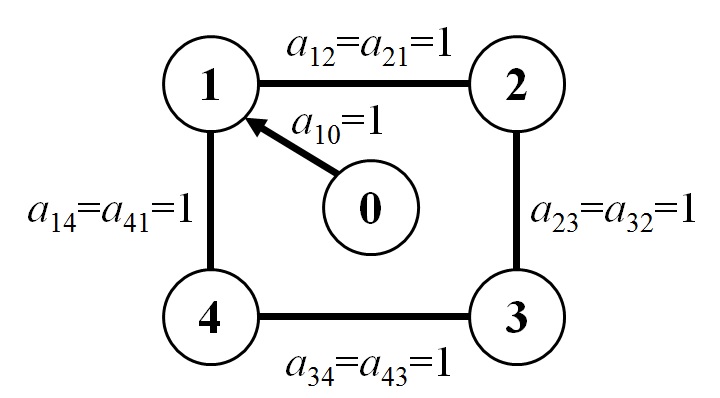
Figure 1: Communication graph of the leader-following system

In the following, the performance of the proposed distributed control methods are demonstrated through a simulated leader-following spacecraft system with four identical rigid spacecraft as followers. The leader’s attitude trajectory is described by $Q_{0}(0)=\textbf{1}$ and $\omega_{0}(t)=0.01[\sin(\Omega_{0}t),\cos(\Omega_{0}t),\sin(\Omega_{0}t)]^{T}$ rad/s, where $\Omega_{0}=0.01$ rad/s. The inertia of the follower spacecraft is given by $J_{i}=\textup{diag}(10,8,12)\,\textup{kg}\cdot\textup{m}^{2}$, $i\in\mathbb{I}_{n}$. Three numerical examples are presented, namely, 1) simulations without any uncertainty, 2) simulations with communication and measurement delays as well as external disturbances, and 3) simulations with time-varying topologies. The simulations are conducted in MATLAB/Simulink using the default integrator ode45 with a maximum step size of 0.001 s.

V-A Simulations without Any Uncertainty

In this section, simulations are conducted with zero disturbance and instantaneous communication between neighboring spacecraft. Assume that the communication graph $\bar{G}$ is fixed and all nonzero edge weights are given in Fig. 1. The measurement and communication frequencies of each spacecraft are both set to 100 Hz. The initial attitudes and angular velocities of the four followers are given by

$$\begin{matrix}\begin{bmatrix}Q_{1}^{T}(0)\\ Q_{2}^{T}(0)\\ Q_{3}^{T}(0)\\ Q_{4}^{T}(0)\end{bmatrix}&=&\begin{bmatrix}0&1&0&0\\ 0&0&-1&0\\ 0.6164&0.5&-0.6&0.1\\ -0.8426&-0.2&0.3&0.4\end{bmatrix}\end{matrix}$$

$$\begin{matrix}\begin{bmatrix}\omega_{1}^{T}(0)\\ \omega_{2}^{T}(0)\\ \omega_{3}^{T}(0)\\ \omega_{4}^{T}(0)\end{bmatrix}&=&\begin{bmatrix}0.2&0.2&0.2\\ -0.1&-0.1&-0.1\\ 0.4&0.4&0.4\\ -0.3&-0.3&0.3\end{bmatrix}\end{matrix}\,\textup{rad/s}$$

The first set of simulations assume that the attitude and angular velocity of each follower are available. Controller (23) and the distributed observer given in (7)-(10) are applied. The corresponding control parameters are summarized in Table I. Figure 2 shows the estimation errors of the leader’s quaternion, angular velocity, and acceleration in terms of their respective 2-norms. As shown by Fig. 2, the proposed distributed observer exhibits fast transient and each follower recovers the leader’s attitude, angular velocity, and acceleration within 5 s. Since both $P_{0}$ and $-P_{0}$ represent the leader’s attitude, Fig. 3 compares the responses of $\|P_{i}-P_{0}\|$ and $\|P_{i}+P_{0}\|$. At the beginning $P_{4}$ is much closer to $-P_{0}$ but the observer still stabilizes $P_{4}$ through a longer path to $P_{0}$ instead of $-P_{0}$. Therefore, the unwinding phenomenon occurred in the distributed observer. Fortunately, this problem does not degrade the performance of the consensus controllers due to their global stabilizing feature, as shown by Figs. 4 and 5 later. Figure 4 depicts the time histories of the attitude tracking error $\eta_{i0}(t)$, 2-norm of the angular velocity tracking error $\|\omega_{i0}(t)\|_{2}$, and the control torque component $\tau_{i1}$. It can be seen that the proposed full-state feedback consensus scheme successfully aligns the attitude of each follower with the dynamic leader through the shortest path in finite-time.

Next, the angular velocity measurements are removed from all followers and the velocity-free controller (27) is simulated under the same initial conditions. The control gains are shown in Table I. Figure 5 presents the responses of $\eta_{i0}(t)$, $\|\omega_{i0}(t)\|_{2}$ and $\tau_{i1}$. The followers also reach an agreement with the leader in finite time, though there is no angular velocity measurements. Compared to the full-sate feedback case, the angular velocity tracking error in Fig. (5) exhibits increased transients. This is mainly caused by the weakened damping effect due to the lack of velocity measurements for feedback control.

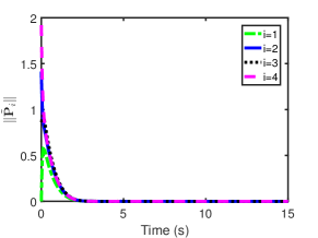
(a)

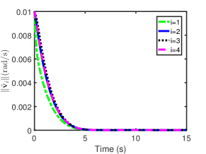
(b)

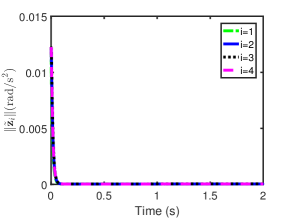
(c)

Figure 2: Response of the distributed observer without any uncertainty: (a) $\|\tilde{P}_{i}\|_{2}$, (b) $\|\tilde{v}_{i}\|_{2}$, and (c) $\|\tilde{z}_{i}\|_{2}$

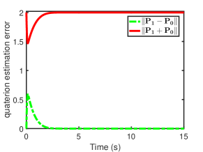
(a)

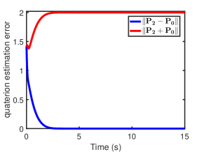
(b)

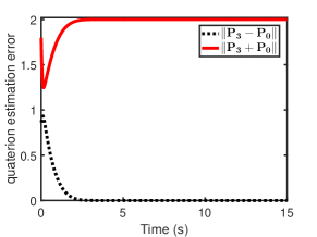
(c)

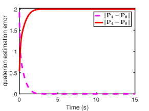
(d)

Figure 3: The leader’s attitude estimation error $\|P_{i}-P_{0}\|$ and $\|P_{i}+P_{0}\|$ , $i\in\mathbb{I}_{4}$

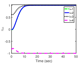
(a)

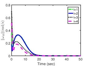
(b)

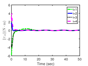
(c)

Figure 4: Simulation results using full-state feedback without any uncertainty: (a) $\eta_{i0}$, (b) $\|\tilde{\omega}_{i0}\|_{2}$, and (c) $\tau_{i1}$

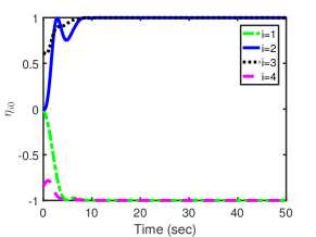
(a)

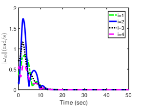
(b)

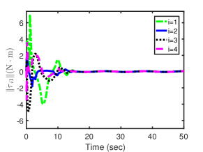
(c)

Figure 5: Simulation results using attitude-only feedback without any uncertainty: (a) $\eta_{i0}$, (b) $\|\tilde{\omega}_{i0}\|_{2}$, and (c) $\tau_{i1}$

V-B Simulations with Time Delays and Disturbances

In order to examine the robustness of the proposed methods, the measurement and communication updates of each spacecraft are delayed by 0.01 s. Additionally, we add a nonzero disturbance torque $d_{i}(t)=0.02[\cos(\theta_{i}t),\sin(\theta_{i}t),-\sin(\theta_{i}t)]^{T}\,\text{N}\cdot\text{m}$, where $\theta_{i}=2\pi/(40+5i)$, $i\in\mathbb{I}_{n}$, to the $i$-th spacecraft. The control parameters remain the same as the previous example while the initial conditions of the four followers are renewed to

$$\begin{matrix}\begin{bmatrix}Q_{1}^{T}(0)\\ Q_{2}^{T}(0)\\ Q_{3}^{T}(0)\\ Q_{4}^{T}(0)\end{bmatrix}&=&\begin{bmatrix}0.3162&0.1&-0.8&0.5\\ -0.1732&-0.5&0.6&-0.6\\ 0.7416&0.5&-0.2&-0.4\\ -0.6557&0.5&-0.4&0.4\end{bmatrix}\end{matrix}$$

$$\begin{matrix}\begin{bmatrix}\omega_{1}^{T}(0)\\ \omega_{2}^{T}(0)\\ \omega_{3}^{T}(0)\\ \omega_{4}^{T}(0)\end{bmatrix}&=&\begin{bmatrix}0.2&-0.1&0.4\\ -0.5&0.6&-0.6\\ -0.5&0.4&-0.2\\ -0.1&-0.6&0.1\end{bmatrix}\end{matrix}\,\textup{rad/s}$$

The simulation results of the distributed observer and full-state feedback controller are presented in Figures 6 and 7. In particular, Fig. 6 shows the estimation errors of the leader’s quaternion, angular velocity, and acceleration in terms of their respective 2-norms while Fig. 7 plots the time histories of $\eta_{i0}(t)$, $\|\omega_{i0}(t)\|_{2}$, and $\tau_{i1}$. In spite of the time delays and external disturbances, the proposed distributed observer still maintains fast transient and each follower obtains the leader’s trajectory with high accuracy within 5 s. The full-state feedback controller successfully synchronizes the attitude of each follower with the dynamic leader (Figs. 7a and 7b). From Fig. 7c, it can be observed that jumps occur in the control torques of followers 2 and 4 as time approaches 1 s while the control torques of followers 1 and 3 remain continuous during the entire control phase. Figure 8 presents the responses of $\eta_{i0}(t)$, $\|\omega_{i0}(t)\|_{2}$ and $\tau_{i1}$ for the attitude-only feedback controller. Similarly to the full-state feedback case, the control torques of followers 2 and 4 switched once before 1 s to change the rotation direction (Fig. 8c). By means of controller (27), the followers reach an agreement with the leader while avoiding the unwinding phenomenon, despite the absence of angular velocity feedback (Figs. 8a and 8b). The simulation results shows that the proposed methods possess some robustness to small time delays and disturbances.

(a)

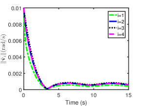
(b)

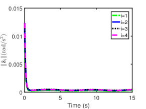
(c)

Figure 6: Response of the distributed observer with time delays and disturbances: (a) $\|\tilde{P}_{i}\|_{2}$, (b) $\|\tilde{v}_{i}\|_{2}$, and (c) $\|\tilde{z}_{i}\|_{2}$

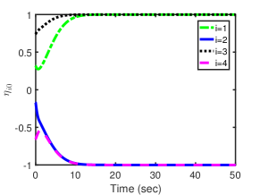
(a)

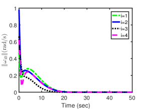
(b)

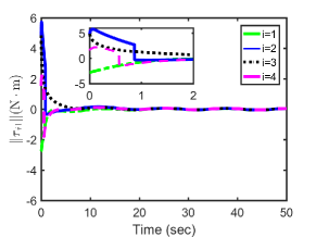
(c)

Figure 7: Simulation results using full-state feedback with time delays and disturbances: (a) $\eta_{i0}$, (b) $\|\tilde{\omega}_{i0}\|_{2}$, and (c) $\tau_{i1}$

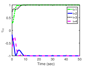
(a)

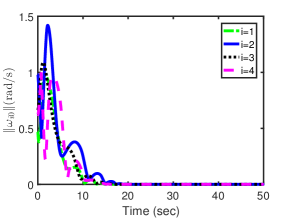
(b)

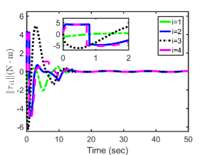
(c)

Figure 8: Simulation results using attitude-only feedback with time delays and disturbances: (a) $\eta_{i0}$, (b) $\|\tilde{\omega}_{i0}\|_{2}$, and (c) $\tau_{i1}$

V-C Simulations with Time-Varying Topologies

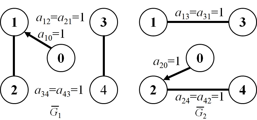
Figure 9: Communication graph of the leader-following system

Although the design in this paper and the previous two examples both assume fixed communication topologies among the multi-spacecraft system, it is still interesting the see how the proposed methods behave with time-varying communication topologies. An example is shown in Fig. 9, the graph $\bar{G}(t)$ has two possible topologies $\bar{G}_{1}$ and $\bar{G}_{2}$. Let $\bar{G}(t)=\bar{G}_{1}$ for $t\in[mt_{D},mt_{D}+0.5t_{D})$ and $\bar{G}(t)=\bar{G}_{2}$ for $t\in[mt_{D}+0.5t_{D},(m+1)t_{D})$, where $t_{D}=0.2$ s and $m=0,1,2,\cdots$. Clearly, the graph $\bar{G}(t)$ is not connected at any moment but the union graph $\bigcup_{t\in[t,t+t_{D})}\bar{G}(t)$ is connected for any $t\geq 0$. Hence, $\bar{G}(t)$ satisfies the joint strong connectivity [1], a condition that is usually employed to guarantee consensus in multi-agent systems with time-varying topologies.

In order to clearly see the effect of the switching topology, simulations are conducted without external disturbance and time delays in measurements and communications. The observer and controller gains are given in Table I while the initial attitudes and angular velocities remain the same as those in Section V.B. The simulation results are presented in Figs. 10–12, showing the responses of the distributed observer, the full-state feedback controller, and the attitude-only controller, respectively. It can be seen that the estimation errors and attitude tracking errors are still convergent with the considered switching topologies. The numerical results inspire us to conjecture that the proposed distributed observer and controller also applies to time-varying topologies satisfying the joint strong connectivity. A rigorous proof of this conjecture is left for future research.

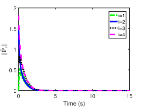
(a)

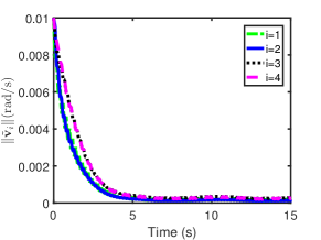
(b)

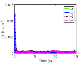
(c)

Figure 10: Response of the distributed observer with time-varying topologies: (a) $\|\tilde{P}_{i}\|_{2}$, (b) $\|\tilde{v}_{i}\|_{2}$, and (c) $\|\tilde{z}_{i}\|_{2}$

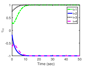
(a)

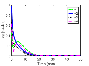
(b)

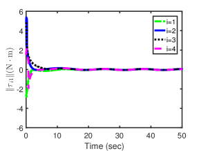
(c)

Figure 11: Simulation results using full-state feedback with time-varying topologies: (a) $\eta_{i0}$, (b) $\|\tilde{\omega}_{i0}\|_{2}$, and (c) $\tau_{i1}$

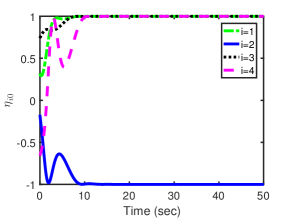
(a)

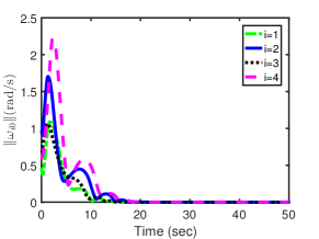
(b)

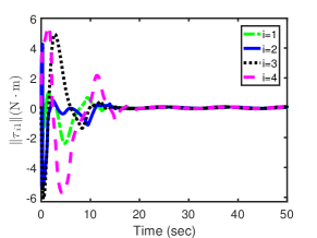
(c)

Figure 12: Simulation results using attitude-only feedback with time-varying topologies: (a) $\eta_{i0}$, (b) $\|\tilde{\omega}_{i0}\|_{2}$, and (c) $\tau_{i1}$

VI Conclusions

Quaternion-based attitude consensus schemes were proposed for a group of leader-following spacecraft with an undirected and connected communication graph among the followers. Instrumental in our approach is a nonlinear distributed observer for the leader’s states, which establishes second-order sliding modes for attitude and angular velocity estimation errors and hence recovers the leader’s trajectory in finite time for each follower. By appropriately integrating the observer and two quaternion-based hybrid homogeneous controllers originally developed for single spacecraft, global group attitude agreement was obtained in finite time respectively with full-state measurements and attitude-only measurements. It is worth noting that the proposed distributed observer allows any reference trajectories with bounded time derivatives and can also be combined with many other single-spacecraft attitude controllers to achieve cooperative attitude tracking while pursuing different performance.

Appendix A Proof of Lemmas II.4 and II.5

Proof of Lemma II.4. The first identity of Lemma II.4 can be verified by direct computations and hence is omitted. According the definition of $E(\cdot)$ in (1), it follows that

$$E^{T}(Q^{\prime})Q=-\eta q^{\prime}+\eta^{\prime}q-q^{\prime}\times q=-\textup{vec}(Q^{*}\circ{Q^{\prime}}),$$

which is the transpose of the second identity of Lemma II.4. As a special case, letting $Q=Q^{\prime}$ yields ${Q^{T}}E(Q)=0$.

Proof of Lemma II.5. Next, applying Lemma II.4 one can derive

$$\begin{split}\sum_{i=1}^{n}\sum_{j=1}^{n}b_{ij}{Q_{j}^{T}}E(Q_{i})&=-\sum_{i=1}^{n}\sum_{j=1}^{n}b_{ij}\textup{vec}^{T}(Q_{j}^{*}\circ{Q_{i}})\\ &=-\sum_{j=1}^{n}\sum_{i=1}^{n}b_{ji}\textup{vec}^{T}(Q_{i}^{*}\circ{Q_{j}}).\end{split}$$ (29)

Invoking $b_{ij}=b_{ji}$ and $-\textup{vec}^{T}(Q_{i}^{*}\circ{Q_{j}})=\textup{vec}^{T}(Q_{j}^{*}\circ{Q_{i}})$, it follows from (29) that

$$\sum_{i=1}^{n}\sum_{j=1}^{n}b_{ij}{Q_{j}^{T}}E(Q_{i}) =\sum_{i=1}^{n}\sum_{j=1}^{n}b_{ij}\textup{vec}^{T}(Q_{j}^{*}\circ{Q_{i}})$$

$$=-\sum_{i=1}^{n}\sum_{j=1}^{n}b_{ij}{Q_{j}^{T}}E(Q_{i}),$$

which implies $\sum_{i=1}^{n}\sum_{j=1}^{n}b_{ij}{Q_{j}^{T}}E(Q_{i})=0$.

Appendix B Proof of Theorem III.1

The proof is divided into four steps by showing the convergence of the sliding mode differentiator and $z_{i}$, $v_{i}$, and $P_{i}$ successively.
Step 1: the convergence of (17). When $a_{i0}=0$ (i.e., no direct access to the leader), it follows from (10) that $y_{i}(t)=w_{i}(t)=0$ and $\tilde{w}_{i}=-\dot{\omega}_{0}$. When $a_{i0}=1$ (i.e., direct access to the leader), applying Lemma II.2 to (17) implies that $w_{i}(t)\to z_{0}(t)=\dot{\omega}_{0}(t)$ in a finite time $t_{r}$, i.e, $A_{0}\tilde{w}(t)=0$ for $t\geq t_{r}$.
Step 2: the convergence of $z_{i}$. Consider a Lyapunov function candidate

$$V_{z}=\frac{1}{2}\tilde{z}^{T}(H\otimes I_{3})\tilde{z}$$

which satisfies $V_{z}\geq 0$ and $V_{z}=0$ if and only if $\tilde{z}=0$, since $H$ is positive definite according to Lemma II.1. The time derivative of $V_{z}$ along (16) is computed as

$$\begin{array}[]{cll}\dot{V}_{z}&=&\tilde{z}^{T}(H\otimes I_{3})\dot{\tilde{z}}\\ {}\hfil&=&z_{s}^{T}[-\lambda_{3}\textup{sgn}(z_{s}-A_{0}\tilde{w})-\textbf{1}_{n}\otimes{\dot{z}_{0}}]\end{array}$$ (30)

Note that

$$\begin{array}[]{cll}\dot{V}_{z}&\leq&(\lambda_{3}+\gamma_{3})\|z_{s}\|_{2}\\ {}\hfil&\leq&(\lambda_{3}+\gamma_{3})\bar{\sigma}(H)\|\tilde{z}\|_{2}\\ {}\hfil&\leq&c_{w}\sqrt{V_{z}}\\ {}\hfil&{}&\text{with}\,c_{w}=(\lambda_{3}+\gamma_{3})\bar{\sigma}(H)\sqrt{\frac{2}{\underline{\sigma}(H)}}\end{array}$$

where $\underline{\sigma}(H\otimes I_{3})=\underline{\sigma}(H)$ and $\bar{\sigma}(H\otimes I_{3})=\bar{\sigma}(H)$ are utilized in the above derivations. Invoking the comparison principle [35] then implies that $\tilde{z}(t)$ remains bounded for $t<t_{r}$. For $t\geq t_{r}$, $A_{0}\tilde{w}(t)=0$ and (30) becomes

$$\begin{split}\dot{V}_{z}&=z_{s}^{T}[-\lambda_{3}\textup{sgn}(z_{s})-\textbf{1}_{n}\otimes{\dot{z}_{0}}]\\ &\leq-\lambda_{3}\|z_{s}\|_{1}+\|\dot{z}_{0}\|_{\infty}\|z_{s}\|_{1}\\ &\leq-(\lambda_{3}-\gamma_{3})\|z_{s}\|_{1}\end{split}$$ (31)

where $\dot{z}_{0}=\ddot{\omega}_{0}$ and $\|\ddot{\omega}_{0}\|\leq\gamma_{3}$ are used in deriving (31). $\forall x\in\mathbb{R}^{n}$, Lemma II.3 can be used to show that

$$\|x\|_{2}\leq\|x\|_{1}\leq\sqrt{n}\|x\|_{2}$$

Noting $\underline{\sigma}(H\otimes I_{3})=\underline{\sigma}(H)$ and $\bar{\sigma}(H\otimes I_{3})=\bar{\sigma}(H)$, one obtains $0.5{\underline{\sigma}(H)}\|\tilde{z}\|_{2}^{2}\leq V_{z}\leq 0.5{\bar{\sigma}(H)}\|\tilde{z}\|_{2}^{2}$ and

$$\|z_{s}\|_{1}\geq\|z_{s}\|_{2}=\|(H\otimes I_{3})\tilde{z}\|_{2}\geq\underline{\sigma}(H)\|\tilde{z}\|_{2}.$$

It then follows from (31) that

$$\dot{V}_{z}\leq-c_{z}\sqrt{V_{z}},\;\textup{with}\;c_{z}=(\lambda_{3}-\gamma_{3})\underline{\sigma}(H)\sqrt{\frac{2}{\bar{\sigma}(H)}}.$$

which implies, according to the comparison principle , that $\tilde{z}(t)$ (or, equivalently, $z(t)$) is uniformly bounded and $\tilde{z}(t)=0$ for all $t\geq T_{z}$, where

$$T_{z}=\frac{2\sqrt{V_{z}(\tilde{z}(0))}}{c_{z}}+t_{r}.$$

Step 3: the convergence of $v_{i}$. Similarly, consider the time derivative of $V_{v}=\tilde{v}^{T}(H\otimes I_{3})\tilde{v}/2$ along (15):

$$\dot{V}_{v}=\tilde{v}^{T}(H\otimes I_{3})\dot{\tilde{v}}=-\lambda_{2}v_{s}^{T}\textup{sgn}^{\beta_{2}}(v_{s})+v_{s}^{T}\tilde{z}.$$ (32)

Recall that (31) implies ${V}_{z}(\tilde{z}(t))\leq{V}_{z}(\tilde{z}(0))$ and thus ${\|\tilde{z}(t)\|_{2}}\leq{\gamma_{z}}\triangleq\sqrt{2V_{z}(\tilde{z}(0))/{\underline{\sigma}(H)}}$. In addition, $\underline{\sigma}(H){\|\tilde{v}\|_{2}}\leq\|v_{s}\|_{2}\leq\bar{\sigma}(H){\|\tilde{v}\|_{2}}$ and $0.5{\underline{\sigma}(H)}\|\tilde{v}\|_{2}^{2}\leq V_{v}\leq 0.5{\bar{\sigma}(H)}\|\tilde{v}\|_{2}^{2}$. It then follows from (32) that $\dot{V}_{v}\leq v_{s}^{T}\tilde{z}\leq{\gamma_{z}\|v_{s}\|_{2}}\leq{c_{v0}\sqrt{V_{v}}}$, where $c_{v0}=\gamma_{z}\bar{\sigma}(H)\sqrt{{2}/{\underline{\sigma}(H)}}$, and thus

$$V_{v}(t)\leq\Gamma_{v}(t)\triangleq\left[0.5c_{v0}t+\sqrt{V_{v}(\tilde{v}(0))}\right]^{2},$$

which implies that $\tilde{v}(t)$ cannot escape in finite time and for $t\in[T_{z},\infty)$ (32) reduces to $\dot{V}_{v}=-\lambda_{2}v_{s}^{T}\textup{sgn}^{\beta_{2}}(v_{s})$. Note that $\forall x\in\mathbb{R}^{n}$, Lemma II.3 implies $x^{T}\textup{sgn}^{\beta_{2}}(x)=\sum_{i=1}^{n}|x_{i}|^{1+\beta_{2}}\geq(\sum_{i=1}^{n}|x_{i}|^{2})^{(1+\beta_{2})/2}$. It then follows that

$$\begin{array}[]{cc}\begin{split}\dot{V}_{v}&\leq-\lambda_{2}{\|v_{s}\|_{2}^{1+\beta_{2}}}\\ &\leq-c_{v}V_{v}^{\frac{1+\beta_{2}}{2}}\end{split},&c_{v}=\lambda_{2}\left[\frac{2\underline{\sigma}^{2}(H)}{\bar{\sigma}(H)}\right]^{\frac{1+\beta_{2}}{2}}.\end{array}$$ (33)

and hence $\tilde{V}_{v}(t)\leq\Gamma_{v}(T_{z})$. Noting $\|v\|_{2}\leq\|\tilde{v}\|_{2}+\sqrt{n}\|v_{0}\|_{2}$ and $\|v_{0}\|_{2}\leq\sqrt{3}\gamma_{1}$, one can deduce that $\|\tilde{v}(t)\|_{2},\|v(t)\|_{2}\leq\gamma_{v}$, where $\gamma_{v}=\sqrt{2\Gamma_{v}(T_{z})/{\underline{\sigma}(H)}}+\sqrt{3n}\gamma_{1}$. Noting $0<(1+\beta_{2})/2<1$ and applying again the comparison principle, it follows that $\tilde{v}(t)\to 0$ in a finite time $T_{v}\geq T_{z}$ satisfying $T_{v}-T_{z}\leq{2V_{v}^{(1-\beta_{2})/{2}}(\tilde{v}(T_{z}))}/{c_{v}(1-\beta_{2})}$. Furthermore, an estimation of $T_{v}$ can be obtained as

$$T_{v}\leq T_{z}+\frac{2\Gamma_{v}^{(1-\beta_{2})/2}(T_{z})}{c_{v}(1-\beta_{2})}.$$

Step 4: the convergence of $P_{i}$. The proof can be performed in a manner similar to Step 2. More precisely, we first show the absence of finite escape time for $\tilde{P}(t)$ and then verify the convergence of the reduced system of (14) for $t\geq T_{v}$. To this end, consider a Lyapunov function candidate $V_{p}=\tilde{P}^{T}(H\otimes I_{4})\tilde{P}/2$ and its time derivative along (14):

$$\begin{split}\dot{V}_{p}&=\tilde{P}^{T}(H\otimes I_{4})\dot{\tilde{P}}\\ &=-\lambda_{1}P_{s}^{T}\textup{sgn}^{\beta_{1}}(P_{s})+\frac{1}{2}\sum_{i=1}^{n}P_{si}^{T}[E(\tilde{P}_{i})v_{i}+E(P_{0})\tilde{v}_{i}].\end{split}$$ (34)

Since $\tilde{v}(t)$ and $v(t)$ are uniformly bounded, there exists a constant $\gamma_{v}\geq 0$ such that $\|\tilde{v}(t)\|_{2},\|v(t)\|_{2}\leq\gamma_{v}$. Invoking Lemma II.4 and noting $\|P_{0}\|_{2}=\|Q_{0}\|_{2}=1$, the following inequalities can be shown:

$$\begin{array}[]{rll}P_{si}^{T}E(\tilde{P}_{i})v_{i}&\leq&\|P_{si}\|_{2}\|E(\tilde{P}_{i})\|_{2}\|v_{i}\|_{2}\\ {}\hfil&\leq&\gamma_{v}\|P_{s}\|_{2}\|\tilde{P}_{i}\|_{2}\leq\gamma_{v}\bar{\sigma}(H)\|\tilde{P}\|_{2}^{2},\\ P_{si}^{T}E(P_{0})\tilde{v}_{i}&\leq&\gamma_{v}\bar{\sigma}(H)\|\tilde{P}\|_{2}\\ {}\hfil&\leq&\gamma_{v}\bar{\sigma}(H)[0.25+\|\tilde{P}\|_{2}^{2}].\end{array}$$

It then follows from (34) that $\dot{V}_{p}\leq c_{p0}V_{p}+c_{p1}$, where $c_{p0}={2n\gamma_{v}\bar{\sigma}(H)}/{\underline{\sigma}(H)}$ and $c_{p1}={n\gamma_{v}\bar{\sigma}(H)}/{8}$. Invoking the comparison principle leads to $V_{p}(t)\leq c_{p2}e^{c_{p0}t}-c_{p1}/c_{p0}$, where $c_{p2}=V_{p}(\tilde{P}(0))+c_{p1}/c_{p0}$, and thus $\tilde{P}(t)$ has no finite escape time. For $t\in[T_{v},\infty)$, it follows that $\tilde{v}(t)=0$ and $v_{i}(t)=v_{0}$, $i\in\mathbb{I}_{n}$, and (34) reduces to

$$\begin{split}\dot{V}_{p}&=-\lambda_{1}P_{s}^{T}\textup{sgn}^{\beta_{1}}(P_{s})+\frac{1}{2}\sum_{i=1}^{n}P_{si}^{T}E(\tilde{P}_{i})v_{0}.\end{split}$$

In addition, we can deduce by means of (12) and Lemmas II.4 and II.5 that

$$\begin{split}\sum_{i=1}^{n}P_{si}^{T}E(\tilde{P}_{i})v_{0}&=\sum_{i=1}^{n}\sum_{j=1}^{n}a_{ij}(\tilde{P}_{i}-\tilde{P}_{j})^{T}E(\tilde{P}_{i})v_{0}\\ &=-\sum_{i=1}^{n}\sum_{j=1}^{n}a_{ij}\tilde{P}_{j}^{T}E(\tilde{P}_{i})v_{0}=0\end{split}$$

As a result, derivations similar to (33) can be used to show that $\dot{V}_{p}\leq-c_{p}V_{p}^{(1+\beta_{1})/{2}}$ holds for $t\in[T_{v},\infty)$, where $c_{p}=\lambda_{1}\left[{2\underline{\sigma}^{2}(H)}/{\bar{\sigma}(H)}\right]^{(1+\beta_{1})/{2}}$. Therefore, $\tilde{P}(t)$ (and thus $P(t)$) is uniformly bounded and $\tilde{P}(t)\to 0$ in a finite time $T_{p}\geq T_{v}$ satisfying $T_{p}-T_{v}\leq{2V_{p}^{(1-\beta_{1})/{2}}(\tilde{P}(T_{v}))}/{c_{p}(1-\beta_{1})}$. An estimation of $T_{p}$ is derived as

$$T_{p}\leq T_{v}+\frac{2\left[c_{p2}e^{c_{p0}T_{v}}-c_{p1}/c_{p0}\right]^{\frac{1-\beta_{1}}{2}}}{c_{p}(1-\beta_{1})}.$$ (35)

Summarizing all the above arguments follows the uniform boundedness of $(P_{i}(t),v_{i}(t),z_{i}(t))$ and $(P_{i}(t),v_{i}(t),\\ z_{i}(t))=(Q_{0}(t),\omega_{0}(t),\dot{\omega}_{0}(t))$ for $t\geq T_{p}$, $i\in{\mathbb{I}_{n}}$, thus concluding the results of Theorem III.1.

Appendix C Proof of Lemma IV.1

Given $Q=[\eta,q^{T}]^{T}\in\mathbb{R}^{4}$, it is clear that $\bar{\kappa}_{1}(Q,\alpha)$ is continuous with respect to $Q$ if $\eta\neq\|Q\|_{2}$. In addition, the following identities are straightforward

$$\begin{array}[]{c}\eta^{2}+\|q\|_{2}^{2}=\|Q\|_{2}^{2},\\ 2\|Q\|_{2}(\|Q\|_{2}-\eta)=(\|Q\|_{2}-\eta)^{2}+\|q\|_{2}^{2}.\end{array}$$

It then follows that $\sqrt{2\|Q\|_{2}(\|Q\|_{2}-\eta)}\geq\|q\|_{2}$ and thus

$$\|\bar{\kappa}_{1}(Q,\alpha)\|_{2}\leq{\|q\|_{2}^{1-\alpha}}=\left(\sqrt{\|Q\|_{2}^{2}-\eta^{2}}\right)^{1-\alpha}$$

Therefore, we have

$$\|\bar{\kappa}_{1}(Q,\alpha)\|_{2}\leq\|Q\|_{2}^{1-\alpha}\,\text{and}\,\lim_{\eta\to\|Q\|_{2}}\bar{\kappa}_{1}(Q,\alpha)=0$$

which implies that $\bar{\kappa}_{1}(Q,\alpha)$ is continuous at $\eta=\|Q\|_{2}$ and thus on $\mathbb{R}^{4}$.

Appendix D Proof of Theorem IV.1

Since $u_{i}(\hat{\mathbf{x}}_{fi}(t))=u_{i}(\mathbf{x}_{fi}(t))$ for $t\geq T_{p}$, we only need to show that there is no finite escape time for the closed-loop trajectory $(Q_{i0}(t),\omega_{i0}(t))$. Note that $Q_{i0}(t)\in\mathbb{S}^{3}$ is trivially bounded. Next, consider the positive-definite function $V_{i}=\omega_{i0}^{T}J_{i}\omega_{i0}/2$. For $\hat{\mathbf{x}}_{fi}\in\hat{C}_{fi}$, its time derivative along (5) and (23) is computed as

$$\dot{V}_{i}=\omega_{i0}^{T}[\hat{u}_{fi}-u_{fi}-k_{pi}\bar{\kappa}_{1}(h_{i}\hat{Q}_{i0},1-\alpha_{pi})-k_{di}\textup{sat}_{\alpha_{di}}(\hat{\omega}_{i0})].$$ (36)

Noting that $\|R(\hat{Q}_{i0})\|_{2}=\|\hat{Q}_{i0}\|_{2}^{2}$ and $\|\hat{Q}_{i0}\|_{2}=\|P_{i}\|_{2}$, Assumption II.2 and Lemma IV.1 together with the uniform boundedness of $(P_{i},v_{i},z_{i})$ can then be used to show the uniform boundedness of all terms involved in the bracket of (36). Hence, there exists a constant $\gamma_{u}>0$ such that $\dot{V}_{i}\leq\gamma_{u}\|\omega_{i0}\|_{2}\leq c_{i}\sqrt{V_{i}}$, where $c_{i}=\gamma_{u}\sqrt{2/\underline{\sigma}(J_{i})}$. Invoking the comparison principle and recalling the continuity of $\omega_{i0}(t)$ over jumps, it follows that $\omega_{i0}(t)$ is bounded for $0\leq t<T_{p}$. When $t\geq T_{p}$, $u_{i}(\hat{\mathbf{x}}_{fi}(t))=u_{i}(\mathbf{x}_{fi}(t))$ and the closed-loop equations reduce to a globally finite-time stable system, according to Theorem 3.1 in [20]. Therefore, the statements of Theorem IV.1 follow.

References

• [1] J. Thunberg, W. Song, E. Montijano, Y. Hong, and X. Hu, “Distributed attitude synchronization control of multi-agent systems with switching topologies,” Automatica, vol. 50, pp. 832––840, 2014.
• [2] M. C. VanDyke and C. D. Hall, “Decentralized coordinated attitude control within a formation of spacecraft,” Journal of Guidance, Control, and Dynamics, vol. 29, no. 5, pp. 1101––1109, 2006.
• [3] A. Abdessameud and A. Tayebi, “Attitude synchronization of a group of spacecraft without velocity measurements,” IEEE Transactions on Automatic Control, vol. 54, no. 11, pp. 2642––2648, 2009.
• [4] D. V. Dimarogonas, P. Tsiotras, and K. J. Kyriakopoulos, “Leader-follower cooperative attitude control of multiple rigid bodies,” Systems and Control Letters, vol. 58, no. 6, pp. 429––435, 2009.
• [5] C. G. Mayhew, R. G. Sanfelice, J. Sheng, M. Arcak, and A. R. Teel, “Quaternion-based hybrid feedback for robust global attitude synchronization,” IEEE Transactions on Automatic Control, vol. 57, no. 8, pp. 2122––2127, 2012.
• [6] W. Ren, “Distributed cooperative attitude synchronization and tracking for multiple rigid bodies,” IEEE Transactions on Control Systems Technology, vol. 18, no. 2, pp. 383––392, 2010.
• [7] Z. Meng, W. Ren, and Z. You, “Decentralised cooperative attitude tracking using modified rodriguez parameters based on relative attitude information,” International Journal of Control, vol. 83, no. 12, pp. 2427––2439, 2010.
• [8] A.-M. Zou, “Distributed attitude synchronization and tracking control for multiple rigid bodies,” IEEE Transactions on Control Systems Technology, vol. 22, no. 2, pp. 1329––1346, 2014.
• [9] A.-M. Zou, A. H. J. de Ruiter, and K. D. Kumar, “Distributed finite-time velocity-free attitude coordination control for spacecraft formations,” Automatica, vol. 67, pp. 46––53, 2016.
• [10] Y. Cao, W. Ren, and Z. Meng, “Decentralized finite-time sliding mode estimators and their applications in decentralized finite-time formation tracking,” Systems and Control Letters, vol. 59, no. 9, pp. 522––529, 2010.
• [11] H. Bai, M. Arcak, and J. T. Wen, “Rigid body attitude coordination without inertial frame information,” Automatica, vol. 44, no. 12, pp. 3170––3175, 2008.
• [12] H. Cai and J. Huang, “The leading-following attitude control of multiple rigid spacecraft systems,” Automatica, vol. 50, pp. 1109––1115, 2014.
• [13] ——, “Leader-following attitude consensus of multiple rigid body systems by attitude feedback control,” Automatica, vol. 69, pp. 87––92, 2016.
• [14] W. Ren, “Formation keeping and attitude alignment for multiple spacecraft through local interactions,” AIAA Journal of Guidance, Control and Dynamics, vol. 30, no. 2, pp. 633––638, 2007.
• [15] H. Du, S. Li, and C. Qian, “Finite-time attitude tracking control of spacecraft with application to attitude synchronization,” IEEE Transactions on Automatic Control, vol. 56, no. 11, pp. 2711––2717, 2011.
• [16] J. Lawton and R. W. Beard, “Synchronized multiple spacecraft rotations,” Automatica, vol. 38, no. 8, pp. 1359––1364, 2002.
• [17] S. P. Bhat and D. S. Bernstein, “A topological obstruction to continuous global stabilization of rotational motion and the unwinding phenomenon,” Systems and Control Letters, vol. 39, no. 1, pp. 63––70, 2000.
• [18] N. A. Chaturvedi, A. K. Sanyal, and N. H. McClamroch, “Rigid-body attitude control,” IEEE Control Systems Maggzine, vol. 31, no. 3, pp. 30–51, 2011.
• [19] Y. Igarashi, T. Hatanaka, M. Fujita, and M. W. Spong, “Passivity-based attitude synchronization in se(3),” IEEE Transactions on Control Systems Technology, vol. 17, no. 15, pp. 1119–1133, 2009.
• [20] H. Gui and G. Vukovich, “Global finite-time attitude tracking via quaternion feedback,” Systems and Control Letters, vol. 97, pp. 176–183, 2016.
• [21] Y. Hong, G. Yang, L. Bushnell, and H. Wang, “Global finite-time stabilization: From state feedback to output feedback,” in Proceedings of the 39th IEEE Conference on Decision and Control, Sydney, Australia, 2000, pp. 2908––2913.
• [22] C. G. Mayhew, R. G. Sanfelice, and A. R. Teel, “Quaternion-based hybrid control for robust global attitude tracking,” IEEE Transactions on Automatic Control, vol. 56, no. 11, pp. 2555––2566, 2011.
• [23] Y. Hong, J. Hu, and L. Gao, “Tracking control for multi-agent consensus with an active leader and variable topology,” Automatica, vol. 42, no. 7, pp. 1177––1182, 2006.
• [24] V. Utkin, “On convergence time and disturbance rejection of super-twisting control,” IEEE Transactions on Automatic Control, vol. 58, no. 8, pp. 2013––2017, 2013.
• [25] G. H. Hardy, J. E. Littlewood, and G. Polya, Inequalities.   U. K.: Cambridge University Press, 1952.
• [26] A. F. Filippov, Differential Equations with Discontinuous Right-Hand Side.   Dordrecht, The Netherlands: Kluwer, 1988.
• [27] A. Levant, “Higher-order sliding modes, differentiation and output-feedback control,” International Journal of Control, vol. 76, no. 7–9, pp. 924––941, 2003.
• [28] M. Izadi and A. K. Sanyal, “Rigid body attitude estimation based on the lagrange-d’alembert principle,” Automatica, vol. 50, no. 10, pp. 2570–2577, 2014.
• [29] J. Bohn, A. K. Sanyal, and E. A. Butcher, “Unscented state estimation for rigid body attitude motion with a finite-time stable observer,” in Proceedings of the 55th IEEE Conference on Decision and Control, Las Vegas, NV, USA, 2016, pp. 4698–4703.
• [30] J. Bohn and A. K. Sanyal, “Almost global finite-time stabilization of rigid body attitude dynamics using rotation matrices,” International Journal of Robust and Nonlinear Control, vol. 26, pp. 2008–2022, 2016.
• [31] A. Tayebi, “Unit quaternion-based output feedback for the attitude tracking problem,” IEEE Transactions on Automatic Control, vol. 53, no. 6, pp. 1516––152, 2008.
• [32] Z. Chen and J. Huang, “Attitude tracking and disturbance rejection of rigid spacecraft by adaptive control,” IEEE Transactions on Automatic Control, vol. 54, no. 3, pp. 600––605, 2009.
• [33] A. H. J. de Ruiter, “Spacecraft attitude tracking with guaranteed performance bounds,” AIAA Journal of Guidance, Control and Dynamics, vol. 36, no. 4, pp. 1214––1221, 2013.
• [34] H. Gui and G. Vukovich, “Finite-time angular velocity observers for rigid-body attitude tracking with bounded inputs,” Int. J. Robust. Nonlinear Control, vol. 27, pp. 15–38, 2017.
• [35] H. K. Khalil, Nonlinear Systems, 3rd ed.   Upper Saddle River, NJ: Prentice-Hall, 2002, pp. 303–334.