Evidence combination for a large number of sources

Abstract

The theory of belief functions is an effective tool to deal with the multiple uncertain information. In recent years, many evidence combination rules have been proposed in this framework, such as the conjunctive rule, the cautious rule, the PCR (Proportional Conflict Redistribution) rules and so on. These rules can be adopted for different types of sources. However, most of these rules are not applicable when the number of sources is large. This is due to either the complexity or the existence of an absorbing element (such as the total conflict mass function for the conjunctive-based rules when applied on unreliable evidence). In this paper, based on the assumption that the majority of sources are reliable, a combination rule for a large number of sources, named LNS (stands for Large Number of Sources), is proposed on the basis of a simple idea: the more common ideas one source shares with others, the more reliable the source is. This rule is adaptable for aggregating a large number of sources among which some are unreliable. It will keep the spirit of the conjunctive rule to reinforce the belief on the focal elements with which the sources are in agreement. The mass on the empty set will be kept as an indicator of the conflict. Moreover, it can be used to elicit the major opinion among the experts. The experimental results on synthetic mass functions verify that the rule can be effectively used to combine a large number of mass functions and to elicit the major opinion.

I Introduction

The theory of belief functions (also called Dempster–Shafer Theory, DST) provides effective tools to modele the uncertain information and to combine them using a combination rule. One of the classical combination rule in the belief function framework is the Dempster’s rule [1]. But this rule has been criticized because of its unexpected behavior under some situations enlightened by the famous Zadeh’s example. Smets proposed a modification of Dempster’s rule, often called “conjunctive rule”, where the empty set can be assigned with a non-null mass under the Transferable Belief Model (TBM) [2]. In fact the conjunctive rule is equivalent to the Dempster rule without the normalization process. It has a fast and clear convergence towards a solution.

Smets supports that the mass on the empty set, called also global conflict, can play a role of alarm [2]. When the global conflict is high, it indicates that there is strong disagreement among the sources of mass functions to be fused. However, as observed in [3, 4], the mass on the empty set is not sufficient to exactly describe the conflict since it includes an amount of auto-conflict [5]. Even if the sources are reliable, they can be of high conflict in sense of the mass assigned to the empty set. When using the conjunctive rule, even if there is only a small amount of concordant evidence, the total conflict mass function, i.e. $m(\emptyset)=1$ will be an absorbing element. Consequently, when combining a large number of (incompatible) mass functions using the conjunctive rule, the global conflict may tend to 1. This makes it impossible to reveal the cause of high global conflict. We do not know whether it is due to the sources to fuse or caused by the absorption power of the empty set [3]. In other words, even the combined mass function by the conjunctive rule is $m(\emptyset)\approx 1$, the proposition that the sources are highly conflicting may be incorrect.

In order to rectify the drawbacks of the classical Dempster’s rule and conjunctive rule, many approaches have been made through the modification of the combination rule. However, most of them are not efficient when applied on a large number of sources either due to the ineffective way to handle conflict or the high complexity of the computation. Moreover, the major opinion among all the participants is not easy to found. In some applications such as crowdsourcing, there are usually a large number of sources. An important problem for crowdsourcing systems is to identify the experts who tend to answer the questions correctly among participants. Finding the reliable workers in the system can improve the quality of knowledge one can extract from crowds. One of the most commonly used assumptions in crowdsourcing systems is that the majority of participants can give correct answers. Thus if the major opinion among the participants could be elicited, the reliable workers can be easily found.

We propose in this paper, a conjunctive-based combination rule, named $\mathrm{LNS}$ (stands for Large Number of Sources), in order to aggregate a large number of mass functions. This rule is based on the idea that combining mass functions from different sources is similar to combining opinions from multiple stake-holders in group decision-making. Hence, the more one’s opinion is consistent with the other experts, the more reliable the source is. To build our rule, we assume that all the mass functions available are separable mass functions. A separable mass function can be expressed by a group of simple support mass functions, such as non-dogmatic mass functions. In many applications, the mass assignments are directly in the form of Simple Support Functions (SSF) [6]. Hence, we can group the SSFs in such a way that sources in the same group have the same focal elements or have focal element without conflict. Mass functions in each small group are first fused and then discounted according to the proportions of SSFs in each group. After that the number of mass functions to fuse is the number of groups which is independent of the number of sources. Therefore, the problem brought by the absorbing element (the empty set) using the conjunctive rule can be avoided.

The rest of this paper is organized as follows. In Section 2, some basic knowledge of belief function theory is briefly introduced. The proposed evidence combination approach is presented in detail in Section 3. Numerical examples are employed to compare different combination rules and show the effectiveness of $\mathrm{LNS}$ rule in Section 4. Finally, Section 5 concludes the paper.

II Background

II-A Basic knowledge on the theory of belief functions

We consider $\Theta=\{\theta_{1},\theta_{2},\ldots,\theta_{n}\}$ such as the discernment frame. A mass function is defined on the power set $2^{\Theta}=\{A:A\subseteq\Theta\}$. The mass function $m:2^{\Theta}\rightarrow[0,1]$ is said to be a Basic Belief Assignment (BBA) on $\text{2}^{\Theta}$, if it satisfies:

$$\sum_{A\subseteq\Theta}m(A)=1.$$ (1)

If $m(A)>0$, with $A\in 2^{\Theta}$, $A$ is called a focal element, and the set of focal elements is denoted by $\mathcal{F}$.

The frame of discernment $\Theta$ can also be a focal element. If $\Theta$ is a focal element, the mass function is called non-dogmatic. The mass assigned to the frame of discernment, $m(\Theta)$, is interpreted as a degree of ignorance. In the case of total ignorance, $m(\Theta)=1$. This mass function is also called a vacuous mass function. If there is only one focal element, i.e. $m(A)=1,A\subset\Theta$, the mass function is categorical. Another special case of assignment is named consonant mass functions, where the focal elements include each other as a subset, i.e. if $A,B\in\mathcal{F},A\subset B~{}\text{or}~{}B\subset A$.

In order to combine information sources assumed reliable and cognitively independent, the conjunctive combination is usually used, given by:

$$m_{\mathrm{conj}}(X)=(\operatornamewithlimits{\text{\scalebox{1.4}{\tiny{$\cap$}}⃝}}_{j=1,\cdots,S}m_{j})(X)=\sum\limits_{Y_{1}\cap\cdots\cap Y_{S}=X}\prod_{j=1}^{S}m_{j}(Y_{j}),$$ (2)

where $m_{j}(Y_{j})$ is the mass allocated to $Y_{j}$ by expert $j$. Another kind of conjunctive combination is Dempster’s rule [7] given by:

$$m_{\mathrm{Dempster}}(X)=\begin{cases}0&\text{if}~{}X=\emptyset,\\ \frac{m_{\mathrm{conj}}(X)}{1-m_{\mathrm{conj}}(\emptyset)}&\text{otherwise}.\end{cases}$$ (3)

The item $\kappa\triangleq m_{\mathrm{conj}}(\emptyset)$ is generally called Dempster’s degree of conflict of the combination or the inconsistency of the combination.

The disjunctive rule [8] can be used if we only assume that at least one of the sources is reliable.

If information sources are dependent the cautious rule [9] can be applied. Cautious combination of $S$ non-dogmatic mass functions $m_{j},j=1,2,\cdots,S$ is defined by the BBA with the following weight function:

$$w(A)=\mathop{\wedge}\limits_{j=1}^{S}w_{j}(A),~{}~{}A\in 2^{\Theta}\setminus\Theta.$$ (4)

We thus have

$$m_{\mathrm{Cautious}}(X)=\operatornamewithlimits{\text{\scalebox{1.4}{\tiny{$\cap$}}⃝}}_{A\subsetneq\Theta}A^{\mathop{\wedge}\limits_{j=1}^{S}w_{j}(A)},$$ (5)

where $A^{w_{j}(A)}$ is the simple support function focused on $A$ with weight function $w_{j}(A)$ issued from the canonical decomposition of $m_{j}$. Note also that $\wedge$ is the min operator. Moreover, in the case of dependant sources, the average combination rule can be choosen.

In order to manage the $\kappa$ value by redistributing it on partial ignorance, the Dubois and Prade rule ($\mathrm{DP}$ rule) [10], can be applied. It can be seen as a mixed conjunctive and disjunctive rule.

Moreover the $\mathrm{PCR6}$ proposed by [5] is one of the most popular rule to combine hight conflicting sources.

II-B Discounting process based on source-reliability

When the sources of evidence are not completely reliable, a discounting operation proposed by [6] can be applied. Denote the reliability degree of mass function $m$ by $\alpha\in[0,1]$, then the discounting operation can be defined as:

$$m^{{}^{\prime}}(A)=\begin{cases}\alpha\times m(A)&\forall A\subset\Theta,\\ 1-\alpha+\alpha\times m(\Theta)&\text{if}~{}A=\Theta.\end{cases}$$ (6)

If $\alpha=1$, the evidence is completely reliable and the BBA will remain unchanged. On the contrary, if $\alpha=0$, the evidence is completely unreliable. In this case the so-called vacuous belief function, $m(\Theta)=1$ can be got. It describes our total ignorance.

Before evoking the discounting process, the reliability of each sources should be known. One possible way to estimate the reliability is to use confusion matrices [11]. Generally, the goal of discounting is to reduce global conflict before combination. One can assume that the conflict comes from the unreliability of the sources. Therefore, the source reliability estimation is to some extent linked to the estimation of conflict between sources.

Hence, Martin et al. proposed to use a conflict measure to evaluate the relative reliability of experts [3]. Once the degree of conflict is computed, the relative reliability of the source can be computed accordingly. Suppose there are $S$ sources, $\mathcal{S}=\{s_{1},s_{2},\cdots,s_{S}\}$, the reliability discounting factor $\alpha_{j}$ of source $s_{j}$ can be defined as follows:

$$\alpha_{j}=f\left(\mathrm{Conf}\left(s_{j},\mathcal{S}\right)\right),$$ (7)

where $\mathrm{Conf}\left(s_{j},\mathcal{S}\right)$ quantifies the degree that source $s_{j}$ conflicts with the other sources in $\mathcal{S}$, and $f$ is a decreasing function. The following function is suggested by the authors:

$$\alpha_{j}=\left(1-\mathrm{Conf}\left(s_{j},\mathcal{S}\right)^{\lambda}\right)^{\frac{1}{\lambda}},$$ (8)

where $\lambda>0$.

II-C Simple support functions

Suppose $m$ is a BBA defined on the frame of discernment $\Theta$. If there exists a subset $A\subseteq\Theta$ such that $m$ could be expressed in the following form:

$$m(X)=\begin{cases}w&X=\Theta,\\ 1-w&X=A,\\ 0&\text{otherwise}.\end{cases}$$ (9)

where $w\in\left[0,1\right]$, then the belief function related to BBA $m$ is called a Simple Support Function (SSF) (also called simple mass function) [6] focused on $A$. Such a SSF can be denoted by $A^{w}(\cdot)$ where the exponent $w$ of the focal element $A$ is the basic belief mass (bbm) given to the frame of discernment $\Theta$, $m(\Theta)$. The complement of $w$ to 1, i.e. $1-w$, is the bbm allocated to $A$ [12]. If $w=1$ the mass function represents the total ignorance, if $w=0$ the mass function is a categorical BBA on $A$.

A belief function is separable if it is a SSF or if it is the conjunctive combination of some SSFs [13]. In the work of [13], this kind of separable masses is called u-separable where “u” stands for “unnormalized”, indicating the conjunctive rule is the unnormalized version of Dempster-Shafer rule. The set of separable mass functions is not obvious to obtain. It is easy to see consonant mass functions (the focal elements are nested) are separable.Smets [12] defined the Generalized Simple Support Function (GSSF) by relaxing the weight $w$ to $[0,\infty)$. Those GSSFs with $w\in(1,\infty)$ are called Inverse Simple Support Functions (ISSF). He proved all non-dogmatic mass functions are separable if one uses GSSFs.

III A combination rule for a large number of mass functions

The conjunctive combination rule tries to reinforce the belief on the focal elements with which most of the sources agree. However, in this rule, the empty set is an absorbing element. When combing inconsistent BBAs, the mass assigned to the empty set tends quickly to 1 with the increasing number of sources [3]. Consequently, when using Dempster rule, the gap between $\kappa$ and 1 may rapidly exceed machine precision, even if the combination is valid theoretically. In that case the fused BBAs by the conjunctive rules (normalized or not) and the pignistic probability are inefficient due to the limitation of machine precision. Moreover, the conjunctive combination rule assumes that all the sources are reliable, which is difficult to reach or to verify in real applications.

In the theory of belief functions, the idea to the reinforce belief and the alarm role of the empty set in the conjunctive rule are essential. In order to propose a rule which can be applicable when the number of mass functions to combine is large and keep the previous behavior, the following assumptions are made:

• The majority of sources are reliable;

• The larger extent one source is consistent with others, the more reliable the source is;

• The sources are cognitively independent [8].

Based on these assumptions, the proposed rule will discount the mass functions according to the number of sources providing BBAs with the same focal elements. The discounting factor is directly given by the proportion of mass functions with the same focal elements. As a result, the rule will give more importance to the groups of mass functions that are in a domain, and it is free of auto-conflict [5]. This procedure can be used to elicit of the majority opinion.

The simple support mass functions are considered here. In this case, the mass functions can be grouped in the light of their focal elements (except the frame $\Theta$). To make the rule applicable on separable mass functions, the decomposition process should be performed to decompose each BBA into simple support mass functions. In most of applications, the basic belief can be defined using separable mass functions, such as simple support functions [14] and consonant mass functions [15].

Hereafter we describe the proposed $\mathrm{LNS}$ rule for simple support functions, and then an approximation calculation method of $\mathrm{LNS}$ rule is suggested.

III-A Combination of many simple support functions

Suppose that each evidence is represented by a SSF. Then all the BBAs can be divided into at most $2^{n}$ groups (where $n=|\Theta|$). It is easy to see that there is no conflict at all in each group because of consistency. The focal elements of the SSF are singletons and $\Theta$ itself. For the combination of BBAs inside each group, the conjunctive rule can be employed directly. Then the fused BBAs are discounted according to the number of mass functions in each group. Finally, the global combination of the BBAs of different groups is preformed also using the conjunctive rule. Suppose that all BBAs are defined on the frame of discernment

$$\Theta=\{\theta_{1},\theta_{2},\cdots,\theta_{n}\},$$

and denoted by

$$m_{j}=(A_{i})^{w_{j}},j=1,\cdots,S,i=1,2,\cdots,c,$$

where $c\leq 2^{n}$. The detailed process of the combination is listed as follows. Our proposed rule called $\mathrm{LNS}$ for Large Number of Sources rule is composed of the four following steps:

1. Cluster the simple BBAs into $c$ groups based on their focal element $A_{i}$. For the convenience, each class is labeled by its corresponding focal element.

2. Combine the BBAs in the same group. Denote the combined BBA in group $A_{k}$ by SSF $\hat{m}_{k}=(A_{k})^{\hat{w}_{k}}$, $k=1,2,\cdots,c$. For the conjunctive combination rule we have:

   $$\hat{m}_{k}=\operatornamewithlimits{\text{\scalebox{1.4}{\tiny{$\cap$}}⃝}}_{j=1,\cdots,s_{k}}m_{j}=(A_{k})^{\displaystyle\prod_{j=1}^{s_{k}}w_{j}}$$ (10)

   where the number of BBAs in group $A_{k}$ is $s_{k}$. In order to consider the total ignorance as a neutral element of the rule, if $A_{k}=\Theta$ we allow $s_{k}=0$.

3. Reliability-based discounting. Suppose the fused BBA of all the mass functions in $A_{k}$ be $\hat{m}_{k}$. At this time, each group can be regarded as a source, and there are $c$ sources in total. The reliability of one source can be estimated by comparing to the group of sources. In our opinion, the reliability of source $A_{k}$ is related to the proportion of BBAs in this group. The larger the number of BBAs in group $A_{k}$ is, the more reliable $A_{k}$ is. Then the reliability discounting factor of $\hat{m}_{k}$, denoted by $\alpha_{k}$, can be defined as:

   $$\alpha_{k}=\frac{s_{k}}{\displaystyle\sum_{i=1}^{c}s_{i}}.$$ (11)

   Another version of the discounting factor can be determined by a factor taking into account the precision of the group:

   $$\alpha_{k}=\frac{\beta_{k}^{\eta}s_{k}}{\displaystyle\sum_{i=1}^{c}\beta_{i}^{\eta}s_{i}},$$ (12)

   where

   $$\beta_{k}=\frac{|\Theta|}{|A_{k}|}.$$ (13)

   Parameter $\eta$ can be used to adjust the precision of the combination results. The larger the value of $\eta$ is, the less imprecise the resulting BBA is. The discounted BBA of $\hat{m}_{k}$ can be denoted by SSF $\hat{m}_{k}^{{}^{\prime}}=(A_{k})^{\hat{w}_{k}^{{}^{\prime}}}$ with $\hat{w}_{k}^{{}^{\prime}}=1-\alpha_{k}+\alpha_{k}\hat{w}_{k}$. As we can see, when the number of BBAs in one group is larger, $\alpha$ is closer to 1. That is to say, the fused mass in this group is more reliable.

4. Global combine the fused BBAs in different groups using the conjunctive rule:

   $$m_{\mathrm{LNS}}=\operatornamewithlimits{\text{\scalebox{1.4}{\tiny{$\cap$}}⃝}}_{k=1,\cdots,c}\hat{m}_{k}^{\prime}=\operatornamewithlimits{\text{\scalebox{1.4}{\tiny{$\cap$}}⃝}}_{k=1,\cdots,c}(A_{k})^{\hat{w}_{k}^{{}^{\prime}}}$$ (14)

The previous mentioned methods in Section II-B to estimate reliability are much more complex than the proposed method here. Indeed, usually the distance between BBAs should be calculated or a special learning process is required. In $\mathrm{LNS}$ rule, to evaluate the reliability discounting factor, we only need to count the number of SSFs in each group. But other reliability estimation methods can also be used.

In the last step of combination, as the number of mass functions that takes part in the global combination is small (at most $2^{n}$), other combination rules such as $\mathrm{DP}$ rule [10] and PCR rules [5] are also possible in practice instead of Eq. (14).

III-B LNS properties

The proposed rule is commutative, but not associative. The rule is not idempotent, but there is no absorbing element. The vacuous mass function is a neutral element of the $\mathrm{LNS}$ rule.

There are four steps when applying $\mathrm{LNS}$ rule: decomposition (not necessary for simple support mass functions), inner-group combination, discounting and global combination. The $\mathrm{LNS}$ rule has the same memory complexity as some other rules such as conjunctive, $\mathrm{Dempster}$ and cautious rules if all the rules are combined globally using FMT method. Only $\mathrm{DP}$ and $\mathrm{PCR6}$ rules have higher memory complexity because of the partial conflict to manage. Suppose the number of mass functions to combine is $S$, and the number of elements in the frame of discernment is $n$. The complexity for decomposing mass functions to SSFs is $O(Sn2^{n})$. For combining the mass functions in each group, due to the structure of the simple support mass functions, we only need to calculate the product of the masses on only one focal element $\Theta$. Thus the complexity is $O(S)$. The complexity of the discounting is $O(2^{n})$. In the process of global combination, the BBAs are all SSFs. If we use the Fast Möbuis Transform method, the complexity is $O(n2^{n})$. Moreover there are at most $2^{n}$ mass functions participating the following discounting and global conjunctive combination processes. Since in most application cases with a large number of mass functions, we have $2^{n}\ll S$, the last two steps are not very time-consuming. The total complexity of $\mathrm{LNS}$ is $O(Sn2^{n}+S+2^{n}+n2^{n})$ and so is equivalent to $O(Sn2^{n})$.

We remark here that one of the assumptions of $\mathrm{LNS}$ rule is that the majority of sources are reliable. However, this condition is not always satisfied in every applicative context. Consider here an example with two sensor technologies: TA and TB. The system has two TA-sensors ($S_{1}$ and $S_{2}$), and one TB-sensor $S_{3}$. Suppose also a parasite signal causes TA sensors to malfunction. In this situation, the majority of sensors are unreliable, and we could not get a good result if the $\mathrm{LNS}$ rule is used directly as $\mathrm{LNS}(S_{1},S_{2},S_{3})$ at this time. Actually there is an underlying hierarchy in the sources of information, $\mathrm{LNS}$ rule could be evoked according to the hierarchy, such as $\mathrm{LNS}(\mathrm{LNS}(S_{1},S_{2}),S_{3})$. We will study that more in the future work.

IV Experiments

To illustrate the behavior of the proposed combination rule $\mathrm{LNS}$ and to compare with other classical rules, several experiments will be conducted here. Some different types of randomly generated mass functions will be used. The function RandomMass in R package ibelief [16] is adopted to generate random mass functions.

Experiment 1. In the crowdsourcing applications, all the users can provide some imprecise and uncertain answers. But only a few are trusty. The elicitation of the majority opinion is very important to identify the experts. Assume that the answers by different uses are in the form of the mass functions over the same discernment frame $\Theta=\{\theta_{1},\theta_{2},\theta_{3}\},$ denoted by $m_{j},j=1,2,\cdots,6$. The assignments of all the mass functions are as follows:

$$m_{1}:m_{1}(\{\theta_{2}\})=0.9,~{}m_{1}(\Theta)=0.1,$$

$$m_{2}:m_{2}(\{\theta_{1}\})=0.1,~{}m_{2}(\Theta)=0.9,$$

$$m_{3}:m_{3}(\{\theta_{1}\})=0.2,~{}m_{3}(\Theta)=0.8,$$

$$m_{4}:m_{4}(\{\theta_{1}\})=0.3,~{}m_{4}(\Theta)=0.7,$$

$$m_{5}:m_{5}(\{\theta_{1}\})=0.1,~{}m_{5}(\Theta)=0.9,$$

$$m_{6}:m_{6}(\{\theta_{1}\})=0.2,~{}m_{6}(\Theta)=0.8.$$

As can be seen from the above equations, there are five out of six mass functions ($m_{2},m_{3},m_{4},m_{5},m_{6}$) assigning a large value on $\theta_{1}$, while $m_{1}$ delivers a function strongly committed to another solution. It indicates that the first source is obviously different from the other five sources.

The combination results by conjunctive rule, $\mathrm{Dempster}$ rule, disjunctive rule, $\mathrm{DP}$ rule, $\mathrm{PCR6}$ rule, cautious rule, average rule and the proposed $\mathrm{LNS}$ rule are depicted in Table I. As can be observed, the conjunctive rule assigns most of the belief to the empty set, regarding the sources as highly conflictual. $\mathrm{Dempster}$ rule, $\mathrm{DP}$ rule, $\mathrm{PCR6}$ rule and average rule redistribute all the global conflict to other focal elements. Disjunctive rule gives the total ignorance mass functions. Cautious rule and the proposed $\mathrm{LNS}$ rule keep some of the conflict and redistribute the remaining. From the original six BBAs, we can see that there are five mass functions supporting $\{\theta_{1}\}$, while only one supporting $\{\theta_{2}\}$. The six mass functions are not conflicting, because the majority of evidence shows the preference of $\{\theta_{1}\}$. We consider here source 1 is not reliable since it contradicts with all the other sources. But the belief given to $\{\theta_{2}\}$ is more than that to $\{\theta_{1}\}$ when using $\mathrm{Dempster}$, $\mathrm{DP}$, $\mathrm{PCR6}$, and the cautious rule, which indicates that these rules are not robust to the unreliable evidence. The result by the average rule gives equal evidence to $\{\theta_{1}\}$ and $\{\theta_{2}\}$. The obtained fused BBA by the proposed rule assigns the largest mass to focal element $\{\theta_{1}\}$, which is consistent with the intuition. It keeps a certain level of global conflict, and at the same time reflects the superiority of $\{\theta_{1}\}$ compared with $\{\theta_{2}\}$. From the results we can see that only the $\mathrm{LNS}$ rule can correctly elicit the major opinion.

TABLE I: The combination of six masses. For the names of columns, $\theta_{ij}$ is used to denote $\{\theta_{i},\theta_{j}\}$.

	Conjunctive	DS	Disjunctive	DP	PCR6	Cautious	Average	$\mathrm{LNS}$
$\emptyset$	0.57341	0.00000	0.00000	0.00000	0.00000	0.27000	0.00000	0.07964
$\theta_{1}$	0.06371	0.14935	0.00000	0.06371	0.10644	0.03000	0.15000	0.45129
$\theta_{2}$	0.32659	0.76558	0.00000	0.32659	0.45139	0.63000	0.15000	0.07036
$\theta_{12}$	0.00000	0.00000	0.00011	0.08165	0.00000	0.00000	0.00000	0.00000
$\theta_{3}$	0.00000	0.00000	0.00000	0.00000	0.00000	0.00000	0.00000	0.00000
$\theta_{13}$	0.00000	0.00000	0.00000	0.00000	0.00000	0.00000	0.00000	0.00000
$\theta_{23}$	0.00000	0.00000	0.00000	0.00000	0.00000	0.00000	0.00000	0.00000
$\Theta$	0.03629	0.08506	0.99989	0.03629	0.44217	0.07000	0.70000	0.39871

Experiment 2. We test here the influence of parameters $\eta$ and $\beta$ in $\mathrm{LNS}$ rule. Simple support mass functions are utilized in this experiment. Suppose that the discernment frame under consideration is $\Theta=\{\theta_{1},\theta_{2},\theta_{3}\}$. Three types of SSFs are adopted. First $s_{1}=60$ and $s_{2}=50$ SSFs with focal element $\{\theta_{1}\}$ and $\{\theta_{2}\}$ respectively (the other focal element is $\Theta$) are uniformly generated, and then $s_{3}=50$ SSFs with focal element $\theta_{23}\triangleq\{\theta_{2},\theta_{3}\}$ are generated. The value of masses are randomly generated. Different values of $\eta$ ranging from 0 to 6 are used to test. The mass values in the fused BBA by $\mathrm{LNS}$ varying with $\eta$ are displayed in Figure 1, and the corresponding pignistic probabilities are shown in Figure 2.

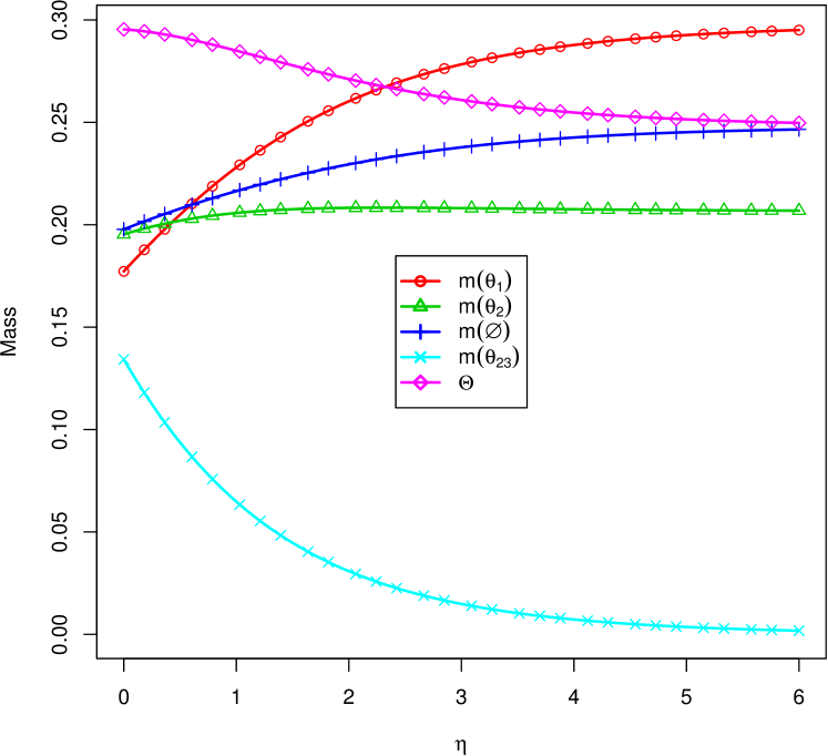
Figure 1: The BBA after the combination for three types of SSFs using $\mathrm{LNS}$ rule. The mass functions are generated randomly, and $\mathrm{LNS}$ rule is evoked with different values of $\eta$ ranging from 0 to 6.

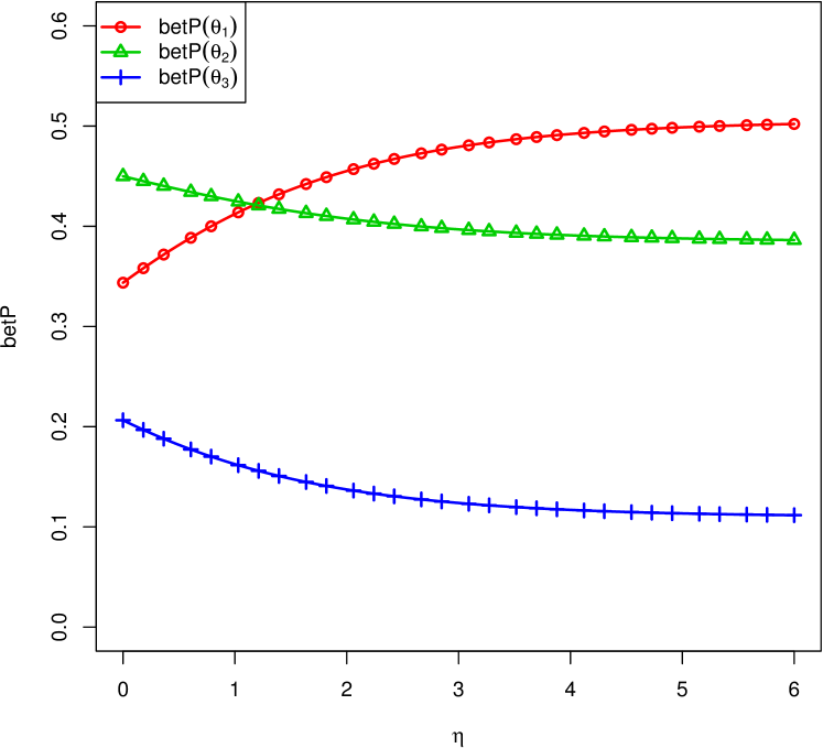
Figure 2: The Pignistic probability after the Combination for three types of SSFs using $\mathrm{LNS}$ rule. The mass functions are generated randomly, and $\mathrm{LNS}$ rule is evoked with different values of $\eta$ ranging from 0 to 6.

From these figures, we can see that $\eta$ can have some effects on the final decision. Figure 1 shows that with the increasing of $\beta$, the mass function assigned to the singleton focal elements increases. On the contrary, the mass given to the focal element whose cardinality is bigger than one decreases. In fact parameter $\beta$ in $\mathrm{LNS}$ aims at weakening the imprecise evidence which gives only positive mass to focal elements with high cardinality, and the exponent $\eta$ allows to control the degree of discounting. If $\eta$ is larger, we give more weights to the sources of evidence whose focal elements are more specific, and more discount will be committed to the imprecise evidence. As a result, in the experiment when $\eta$ is larger than 1.2, $\mathrm{BetP}(\theta_{1})>\mathrm{BetP}(\theta_{2})$ (Figure 2). At this time the mass functions with focal element $\{\theta_{2},\theta_{3}\}$ make little contribution to the fusion process, while the final decision mainly depends on the other two types of simple support mass functions with singletons as focal elements.

In real applications, $\eta$ could be determined based on specific requirement. This work is not specially focusing on how to determine $\eta$, thus in the following experiment we will set $\eta=1$ as default.

Experiment 3. The goal of this experiment is to show how Dempster’s degree of conflict is dealt with by most of rules when combining a large number of conflicting sources.

In this experiment, the frame of discernment is set to $\Theta=\{\theta_{1},\theta_{2}\}$. Assume that there are only 2 focal elements on each BBA. One is the whole frame $\Theta$, and the other is any of the singletons ($\{\theta_{1}\}$ or $\{\theta_{2}\}$). The number of BBAs which have the focal element $\{\theta_{1}\}$ is set to $s_{1}$, while that with $\{\theta_{2}\}$ is $s_{2}$. We fix the value of $s_{2}$, and let $s_{1}=t*n_{2}$, with $t$ a positive integer. We generate $S=s_{1}+s_{2}$ such kind of BBAs randomly, but only withholding the BBAs for which the mass value assigned to $\{\theta_{1}\}$ or $\{\theta_{2}\}$ is greater than 0.5.

Four values of $t$ are considered here: $t=1,2,3,4$. If $t=1$, $s_{1}=s_{2}=S/2$. If $t=2$, the number of mass functions supporting $\{\theta_{1}\}$ is two times of that supporting $\{\theta_{2}\}$, and so on. The global conflict (mass given to the empty set) after the combination with different values of $s_{2}$ for the four cases is displayed in Figures 3–6 respectively. The mass assigned to the focal element $\{\theta_{1}\}$ with different combination approaches is shown in Figures 7–10.

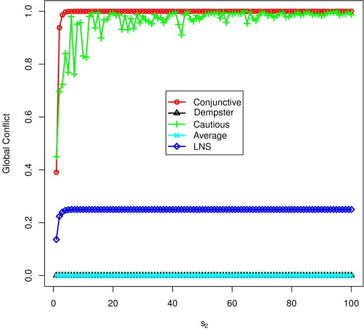
Figure 3: The global conflict after the combination with $s_{1}=s_{2}$.

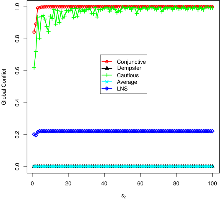
Figure 4: The global conflict after the combination with $s_{1}=2*s_{2}$.

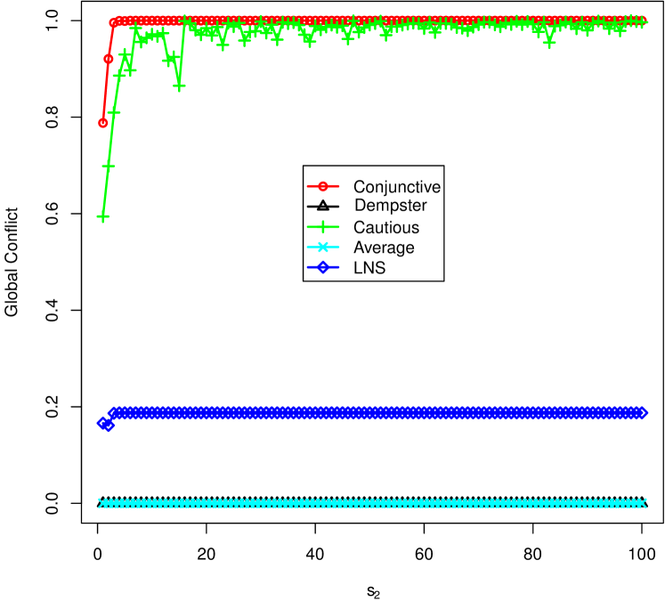
Figure 5: The global conflict after the combination with $s_{1}=3*s_{2}$.

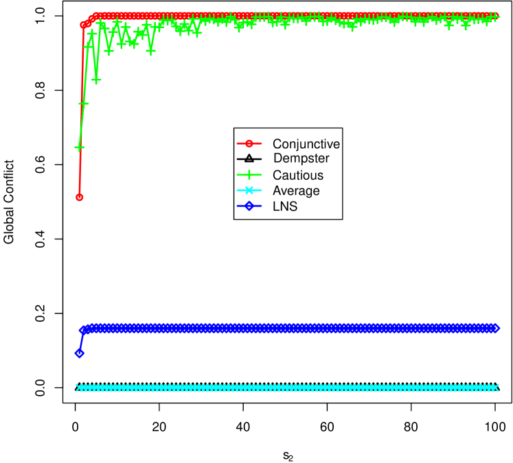
Figure 6: The global conflict after the combination with $s_{1}=4*s_{2}$.

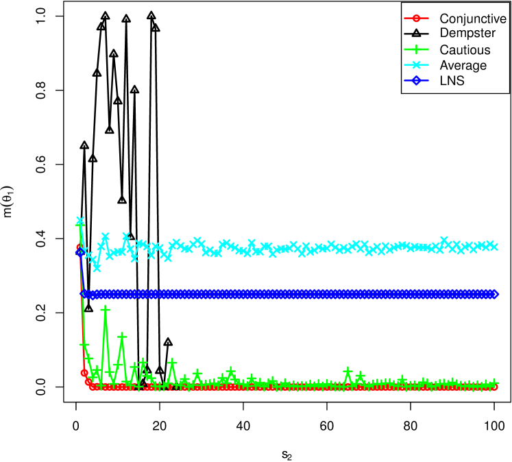
Figure 7: The mass on $\{\theta_{1}\}$ after the combination with $s_{1}=s_{2}$.

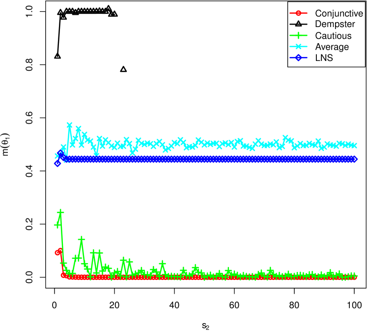
Figure 8: The mass on $\{\theta_{1}\}$ after the combination with $s_{1}=2*s_{2}$.

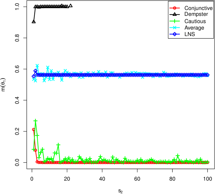
Figure 9: The mass on $\{\theta_{1}\}$ after the combination with $s_{1}=3*s_{2}$.

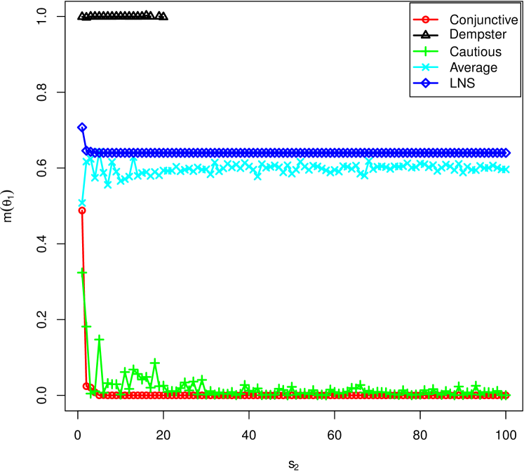
Figure 10: The mass on $\{\theta_{1}\}$ after the combination with $s_{1}=4*s_{2}$.

It is intuitive that when $t$ becomes larger, the global conflict should be smaller and we should give more belief to the focal element $\{\theta_{1}\}$. From Figures 3–10 we can see that only the results by $\mathrm{LNS}$ rule are in accordance with this common sense. The simple average rule assigns larger BBA to $\{\theta_{1}\}$, but it does not keep any conflict. $\mathrm{Dempster}$ rule could not work at all when $s_{2}$ is larger than 20, as it regards these BBAs as highly conflict. Although the conjunctive rule and cautious rule could work when combining a larger number of mass functions, the obtained fused mass function is $m(\emptyset)\approx 1$, which is useless for decision in practical.

From Figures 3–6, we can see a kind of limit of the global conflict for the $\mathrm{LNS}$ rule. In fact, the mass on the empty set for this rule is also depending on the size of the frame of discernment and more directly on the number of groups created in the first step of the rule. The limit value of the global conflict will tend to 1 with the increase of the size of discernment when considering only categorical BBAs on different singletons.

V Conclusion

There is usually a lot of uncertain information in big data applications. The theory of belief functions is a flexile framework to deal with imprecise and uncertain information, especially it provides many ways for the task of information fusion. However, although lots of combination rules have been designed in recent years in this framework, most of them are not applicable when the number of source to combine is quite large due to the complexity or the existing absorbing element.

We propose here a new combination rule, named $\mathrm{LNS}$ rule, preserving the principle of the conjunctive rule. This rule first groups the mass functions according to their set of focal elements (without auto-conflict). After the inner combination, the mass functions in each group can be summarized by one mass function. The reliability of the source is estimated by the proportion of BBAs in one group. Therefore, after discounting the mass function of each group by the reliability factor, the final combination can be proceeded by the conjunctive rule (or another rule according to the application).

The $\mathrm{LNS}$ rule is able to combine a large number of mass functions. The only existing method applicable for a large number of sources is the average rule. However, that rule may give more importance to few sources with a high belief (even if the source is not reliable). It cannot capture the conflict between the sources. The proposed rule has a reasonable complexity (lower than the $\mathrm{DP}$ and $\mathrm{PCR6}$ rules). Moreover, it can provide reasonable combination results and can be used to elicit the major opinion. This is of practical value in the crowdsourcing system.

Overall, this work provides a perspective for the application of belief functions on big data. We will study how to apply $\mathrm{LNS}$ rule on the problems of social network and crowdsourcing in the future research work.

References

- [1] P. Smets, “Analyzing the combination of conflicting belief functions,” Information Fusion, vol. 8, pp. 387–412, 2007.
- [2] ——, “The combination of evidence in the transferable belief model,” Pattern Analysis and Machine Intelligence, IEEE Transactions on, vol. 12, no. 5, pp. 447–458, 1990.
- [3] A. Martin, A.-L. Jousselme, and C. Osswald, “Conflict measure for the discounting operation on belief functions,” in Information Fusion, 2008 11th International Conference on. IEEE, 2008, pp. 1–8.
- [4] S. Destercke and T. Burger, “Toward an axiomatic definition of conflict between belief functions,” Cybernetics, IEEE Transactions on, vol. 43, no. 2, pp. 585–596, 2013.
- [5] A. Martin and C. Osswald, “Human experts fusion for image classification,” Information & Security: An International Journal, Special issue on Fusing Uncertain, Imprecise and Paradoxist Information (DSmT), vol. 20, pp. 122–143, 2006.
- [6] G. Shafer, A mathematical theory of evidence. Princeton University Press, 1976.
- [7] A. P. Dempster, “Upper and lower probabilities induced by a multivalued mapping,” The annals of mathematical statistics, pp. 325–339, 1967.
- [8] P. Smets, “Belief functions: the disjunctive rule of combination and the generalized bayesian theorem,” International Journal of approximate reasoning, vol. 9, no. 1, pp. 1–35, 1993.
- [9] T. Denœux, “The cautious rule of combination for belief functions and some extensions,” in Information Fusion, 2006 9th International Conference on. IEEE, 2006, pp. 1–8.
- [10] D. Dubois and H. Prade, “Representation and combination of uncertainty with belief functions and possibility measures,” Computational Intelligence, vol. 4, no. 3, pp. 244–264, 1988.
- [11] A. Martin, “Comparative study of information fusion methods for sonar images classification,” in Information Fusion, 2005 8th International Conference on, vol. 2. IEEE, 2005, pp. 7–pp.
- [12] P. Smets, “The canonical decomposition of a weighted belief,” in 14th International Joint Conference on Artificial Intelligence, vol. 95, 1995, pp. 1896–1901.
- [13] T. Denœux, “Conjunctive and disjunctive combination of belief functions induced by nondistinct bodies of evidence,” Artificial Intelligence, vol. 172, no. 2, pp. 234–264, 2008.
- [14] ——, “A –nearest neighbor classification rule based on dempster-shafer theory,” Systems, Man and Cybernetics, IEEE Transactions on, vol. 25, no. 5, pp. 804–813, 1995.
- [15] D. Dubois and H. Prade, “Consonant approximation of belief functions,” International Journal of Approximate Reasoning, vol. 4, no. 5-6, pp. 419–449, 1990.
- [16] K. Zhou and A. Martin, ibelief: Belief Function Implementation, 2015, R package version 1.2. [Online]. Available: http://CRAN.R-project.org/package=ibelief