Attacks and Infections in Percolation Processes

Abstract

We discuss attacks and infections at propagating fronts of percolation processes based on the extended general epidemic process. The scaling behavior of the number of the attacked and infected sites in the long time limit at the ordinary and tricritical percolation transitions is governed by specific composite operators of the field-theoretic representation of this process. We calculate corresponding critical exponents for tricritical percolation in mean-field theory and for ordinary percolation to 1-loop order. Our results agree well with the available numerical data.

I Introduction

A very basic and largely open question in percolation theory is following Gra2012 : what are the scaling properties of the number of the attacked and infected sites at propagating fronts of percolation processes in the long time limit? Here, we study this question in the framework of dynamical field theory of percolation.

To set the stage, to introduce concepts and define terms, it is helpful to think initially in terms of the lattice model known as the extended general epidemic process (EGEP) JMS04 . Usually, dynamical percolation theory is based on the general epidemic process (GEP) Mol77 ; Bai75 ; Mur89 ; Gra83 ; Ja85 ; CaGra85 ; JaTa05 . Several years ago, we generalized the GEP to the EGEP to allow, besides critical percolation, for tricritical and first-order percolation transitions, which had been predicted earlier from simulations in the context of depinning transitions of driven surfaces in random media at zero temperature robbinsEtAl . Simulations also showed that tricritical and first-order percolation disappear below three spatial dimensions in random media depinning DroDa98 as well as in direct simulations of the EGEP BiPaGra2012 .

The EGEP can be viewed as an extension of the well known susceptible-infected-removed (SIR) model kerMcK1927 and is also referred to as the susceptible-weak-infected-removed (SWIR) model. It is given by the reaction scheme

$$S(\mathbf{n})+I(\mathbf{m})\quad \overset{\alpha}{\longrightarrow}\quad I(\mathbf{n})+I(\mathbf{m})\,,$$ (1a)

$$S(\mathbf{n})+I(\mathbf{m})\quad \overset{\beta}{\longrightarrow}\quad W(\mathbf{n})+I(\mathbf{m})\,,$$ (1b)

$$W(\mathbf{n})+I(\mathbf{m})\quad \overset{\gamma}{\longrightarrow}\quad I(\mathbf{n})+I(\mathbf{m})\,,$$ (1c)

$$I(\mathbf{n})\quad \overset{\lambda}{\longrightarrow}\quad R(\mathbf{n})\,.$$ (1d)

with reaction rates $\alpha$, $\beta$, $\gamma$, and $\lambda$. $S$, $W$, $I$, and $R$ respectively denote susceptible, weak, ill (activated), and removed (dead, immune, the debris) individuals on nearest neighbor sites $\mathbf{n}$ and $\mathbf{m}$. A susceptible individual may be infected by an ill neighbor (agent) with rate $\alpha$ [reaction (1a)], or it may be weakened without becoming ill with rate $\beta$ [reaction (1b)]. An attack is defined as any such attempt to either infect or weaken a susceptible neighbor. A further contact of a weak individual with an agent leads then to an infection with rate $\gamma>\alpha$ [reaction (1c)]. By these contagions, the disease spreads diffusively footnote1 . Agents die with a rate $\lambda$ [reaction (1d)]. Figure 1 shows a sketch of the process.

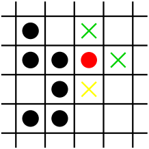
Figure 1: Part of a planar or spherical percolation front propagating from left to right. Red: an activated cell (the agent), black: inactive agents, green: susceptible sites, yellow: weakened site. Both, the susceptible sites and the weakened site, are attackable. In the next time step the agent is deactivated, and zero, one, two or three of the attackable places become agents. Note the asymmetry of the number of the attackable sites in the direction of the propagating front.

As mentioned above, the EGEP features first order, second order and tricritical phase transitions depending on the reaction rates. The second order transition belongs to the universality class of dynamic isotropic percolation (dIP), and the tricitical transition belongs to the universality class of tricritical dynamic isotropic percolation (TdIP). Through previous field theoretic studies Ja85 ; CaGra85 ; JMS04 , much is known about the critical behavior of these universality classes. Most notably, the basic critical exponents such as exponents of order parameters, correlation length and the dynamical exponent have been calculated to 2-loop order.

In the following, we use the physical picture emanating from the EGEP to identify operators in the field theory of dIP and TdIP that describe the scaling properties of the number of the attacked and infected sites in the long time limit. It turns out that these operators are composite operators (local products of fields and their derivatives) whose scaling behavior is not described by the known basic critical exponents of dIP and TdIP. We calculate the scaling exponents of these composite operators for the tricritical percolation transition in mean-field (MF) theory and for the ordinary percolation transition to 1-loop order and we compare our results with the available numerical data.

II Dynamical percolation and the extended general epidemic process

Here, we briefly review some of the basics of dIP, TdIP and the EGEP to provide some more background information, in particular, on their interrelation.

II.1 The essence of isotropic percolation

The essence of isotropic percolation processes can be summarized by four statements describing the universal features of the evolution of such processes on a homogeneous substrate. Let us use the language of an epidemic. Denoting the density of the agents (the activated substrate) $I$ by $n(\mathbf{r},t)$ and the density of the debris $R$ by $m(\mathbf{r},t)$, these four statements read:

1. There is a manifold of absorbing states with $n\equiv 0$ and corresponding distributions of $m$ depending on the history of $n$. All these absorbing states correspond to the extinction of the epidemic.

2. The substrate becomes activated (infected) depending on the density of agents and the density of the debris. This mechanism introduces memory into the process. The debris ultimately stops the disease locally. However, it is possible that the activation is strengthened by the debris through some mechanism (e.g. prior sensibilization of the substrate by an exposure to the agents).

3. The process (the disease) spreads out diffusively by contamination. The agents become deactivated to immune debris after a short time.

4. There are no other slow variables. Microscopic degrees of freedom can be summarized into a local noise or Langevin force $\zeta(\mathbf{r},t)$ respecting the first statement (i.e., the noise cannot generate agents).

The general form of a Langevin equation formulating these statements is

$$\lambda^{-1}\dot{n} =\nabla^{2}n+R(n,m)\,n+\zeta\,,$$ (2a)

$$m(\mathbf{r},t) =\lambda\int_{-\infty}^{t}n(\mathbf{r},t^{\prime})\,dt^{\prime}\,,$$ (2b)

where $\lambda$ is a kinetic coefficient and the Gaussian noise correlation reads

$$\overline{\zeta(\mathbf{r},t)\zeta(\mathbf{r}^{\prime},t^{\prime})}=\lambda^{-1}Q\big{(}n,m\big{)}\,\delta(\mathbf{r}-\mathbf{r}^{\prime})\,\delta(t-t^{\prime})\,.$$ (3)

The dependence of the rate $R(n,m)$ on the density of the debris $m(\mathbf{r},t)$ describes memory of the process mentioned above. We are interested primarily in the behavior of the process close to percolation, where $n$ and $m$ are small allowing for polynomial expansions $R(n,m)=-(\tau+g_{1}m+g_{2}m^{2}+\ldots)n$, $Q(n,m)=(g_{3}+\ldots)n$. We will revisit this Langevin equation in Sec. II.3.

II.2 The EGEP

When the EGEP takes place on a finite lattice, the manifold of states without any agent is inevitably absorbing. Whether a single initial agent leads to an everlasting epidemic in an infinite system depends on the ratio $\alpha/\lambda$. With $\lambda$ fixed and $\beta=0$, there is a certain value $\alpha=\alpha_{c}$ such that for all $\alpha>\alpha_{c}$ an eternal epidemic (a pandemic) occurs. The probability $P(\alpha)$ for the occurrence of a pandemic as a function of $\alpha$ goes to zero continuously at the critical point $\alpha_{c}$. The behavior of the process near this critical point is in the universality class of dIP.

As we have shown JMS04 , the occurrence of the weak individuals gives rise to an instability that can lead to a discontinuous transition and compact growth of the epidemic if $\gamma$ is greater than a critical value $\gamma_{c}(\alpha,\beta)$. In the enlarged three-dimensional phase space spanned by $\alpha$, $\beta$, and $\gamma$ with fixed $\delta$, there exists a critical surface associated with the usual continuous percolation transition and a surface of first order transitions characterized by a finite jump in the probability $P(\alpha,\beta,\gamma)$ for the occurrence of a pandemic. These two surfaces of phase transitions meet at a line of tricritical points determined in MF theory by

$$\gamma=\gamma_{c}=\alpha(1+\alpha/\beta)\,,\quad\alpha=\alpha_{c}=1/z\,,$$ (4)

where $z$ is the coordination number of the lattice. The behavior of the process near these tricritical points is in the universality class of TdIP. Rather precise numerical verifications of some of the predictions of Ref. JMS04 have been made by Bizhani, Paczuski and Grassberger BiPaGra2012 . These authors also showed that first order and tricritical percolation disappears below three dimensions.

A MF description of the EGEP can be derived by treating the reaction equations (1) as deterministic equations without fluctuations. The latter is described by the system of differential equations

$$\dot{S}(\mathbf{n},t) =-(\alpha+\beta)S(\mathbf{n},t)\Sigma I(\mathbf{n},t)\,,$$ (5a)

$$\dot{W}(\mathbf{n},t) =\bigl{[}\beta S(\mathbf{n},t)-\gamma W(\mathbf{n},t)\bigr{]}\Sigma I(\mathbf{n},t)\,,$$ (5b)

$$\dot{I}(\mathbf{n},t) =\bigl{[}\alpha S(\mathbf{n},t)+\gamma W(\mathbf{n},t)\bigr{]}\Sigma I(\mathbf{n},t)$$

$$-\lambda I(\mathbf{n},t)\,,$$ (5c)

$$\dot{R}(\mathbf{n},t) =\lambda I(\mathbf{n},t)$$ (5d)

governing the dynamics of the different kinds of individuals. Here, $$\Sigma X(\mathbf{n},t):=\sum_{\mathbf{m}}^{nn(\mathbf{n})}X(\mathbf{m},t) \mathbf{n} X$$ denotes the summation over the nearest neighbors of of a quantity defined on lattice points. At each lattice site there is the additional constraint

$$S(\mathbf{n},t)+W(\mathbf{n},t)+I(\mathbf{n},t)+R(\mathbf{n},t)=1\,,$$ (6)

if initially $S(\mathbf{n},0)=1$, $W(\mathbf{n},0)=I(\mathbf{n},0)=R(\mathbf{n},0)=0$. Thus, $S(\mathbf{n},t)$, $W(\mathbf{n},t)$, $I(\mathbf{n},t)$, and $R(\mathbf{n},t)$ can be interpreted as the probabilities of finding the corresponding state at a site $\mathbf{n}$ at time $t$. Note that this constraint is a defining feature of the EGEP. It is valid beyond MF theory.

Equations (5a) and (5b) are readily integrated as functions of $\Sigma R(\mathbf{n},t)=\sum_{\mathbf{m}}^{nn(\mathbf{n})}R(\mathbf{m},t)$. We obtain

$$S(\mathbf{n},t)=\exp\bigl{[}-(\alpha+\beta)\Sigma R(\mathbf{n},t)\bigr{]}$$ (7)

and

$$W(\mathbf{n},t) =\frac{\beta}{\alpha+\beta-\gamma}\Big{\{}\exp\bigl{[}-\gamma\Sigma R(\mathbf{n},t)\bigr{]}$$

$$-\exp\bigl{[}-(\alpha+\beta)\Sigma R(\mathbf{n},t)\bigr{]}\Big{\}}\,,$$ (8)

where the time scale $\lambda$ has been set to unity for simplicity. In a continuum approximation of the lattice points, $\mathbf{n}\rightarrow\mathbf{x}$, the occupation numbers $S$, $W$, $I$, and $R$ change into corresponding densities. We set $R(\mathbf{n},t)\rightarrow m(\mathbf{x},t)$, $I(\mathbf{n},t)\rightarrow n(\mathbf{x},t)\sim\dot{m}(\mathbf{x},t)$, $\Sigma I(\mathbf{n},t)\rightarrow zn(\mathbf{x},t)+l^{2}\nabla^{2}n(\mathbf{x},t)$ with $l$ being a length proportional to the lattice constant. Equation (5c) together with the solutions (7) and (8) then produces the mean field equation of motion of the EGEP ,

$$\frac{\partial n(\mathbf{x},t)}{\partial t} =\Bigg{\{}\frac{(\alpha+\beta)(\alpha-\gamma)}{\alpha+\beta-\gamma}\exp\bigl{[}-(\alpha+\beta)zm(\mathbf{x},t)\bigr{]}$$

$$+\frac{\beta\gamma}{\alpha+\beta-\gamma}\,\exp\bigl{[}-\gamma zm(\mathbf{x},t)\bigr{]}\Bigg{\}}zn(\mathbf{x},t)$$

$$-n(\mathbf{x},t)+\alpha l^{2}\nabla^{2}n(\mathbf{x},t)$$

$$=-\Big{\{}(1-z\alpha)+z^{2}\bigl{[}\alpha(\alpha+\beta)-\beta\gamma\bigr{]}m(\mathbf{x},t)$$

$$+O(m(\mathbf{x},t)^{2})\Big{\}}n(\mathbf{x},t)+\alpha l^{2}\nabla^{2}n(\mathbf{x},t)\,.$$ (9)

These MF equations should be compared with the deterministic part of the Langevin-equation (2). In MF approximation, $\tau$ is proportional to $(1-z\alpha)$, and $g_{1}$ is proportional to $\bigl{(}\alpha(\alpha+\beta)-\beta\gamma\bigr{)}$ and $g_{2}$ and $g_{3}$ are finite positive quantities. Hence $\tau$ vanishes at the percolation threshold, and in addition $g_{1}$ is zero at the tricritical point.

II.3 Response functional

Now, we return to the Langevin-equation (2). Reformulating it as a dynamic response functional Ja76 ; DeDo76 ; Ja92 ; Uwe14 leads to JMS04

$$\mathcal{J}=\int d^{d}x\int dt\,\lambda\tilde{n}\big{(} \lambda^{-1}\partial_{t}-\nabla^{2}+\tau+g_{1}m$$

$$+g_{2}m^{2}-g_{3}\tilde{n}\big{)}n\,,$$ (10)

where $\tilde{n}(\mathbf{x},t)$ is the response field. This response functional as it stands is strictly speaking not a minimal field theoretical model at this stage as we have kept it general enough to encompass both the dIP and the TdIP universality classes. We will review the parameter settings and rescalings that take us to either universality class specifically in a moment. For the ease of the argument, we will refer to $\mathcal{J}$ as the EGEP response functional.

Of course, this dynamic functional can be also derived by pursuing other approaches. For example, one could proceed from the MF equations of motion of the EGEP (9) and incorporate fluctuations by adding an absorbing noise source $\zeta(\mathbf{x},t)$. This again leads to the full set of equations (2,3), and finally to the EGEP response functional (10). Or, as some readers might prefer, one can recast the master-equation corresponding to the reaction scheme of the SWIR (1) as a coherent state path integral (CSPI)-action Doi76 ; GraSche80 ; Pel84 ; Ca97 ; Ca08 ; Uwe14 ; TaHoVo05 ; Wie15 and then integrate out the coherent fields corresponding to $S$, $W$, and $R$ followed by a naïve continuum approximation. After switching to number densities as field variables via the Grassberger transformation and deletion of irrelevant operators, see e.g. JaTa05 , one also arrives at the functional (10). However, we prefer the more universal approach outlined in Sec. II.1 that boils down to a purely mesoscopic stochastic formulation based on the correct order parameters identified through physical insight in the nature of the critical phenomenon JMS04 .

The EGEP response functional contains a redundant parameter. This redundancy is connected to the rescaling transformation

$$n \rightarrow b\,n\,,\quad\tilde{n}\rightarrow b^{-1}\tilde{n}\,,$$ (11a)

$$g_{1} \rightarrow b^{-1}g_{1}\,,\quad g_{2}\rightarrow b^{-2}g_{2}\,,\quad g_{3}\rightarrow bg_{3}\,,$$ (11b)

($b$ is some scaling parameter,) that leaves $\mathcal{J}$ invariant. Note that the combinations $g_{1}g_{3}$ and $g_{2}g_{3}^{2}$ are invariant under this transformation.

At the tricritical point, where $g_{1}$ vanishes in MF theory, we fix the redundancy by choosing $b=g_{3}^{-1}$, and for convenience we abbreviate $g=g_{2}g_{3}^{2}$. There are two critical parameters, namely $\tau$ and $\sigma=g_{1}g_{3}$. The fields scale as $\tilde{n}\sim\mu^{2}$, $n\sim\mu^{d-2}$, and $m\sim\mu^{d-4}$ where $\mu$ is the inverse scaling length and $d$ is the spatial dimension. The scaling of the coupling constant $g\sim\mu^{2(5-d)}$ shows that the upper critical dimension is $d_{c}=5$.

Away from the tricritical point, $g_{1}$ is a finite quantity and $g_{2}$ becomes irrelevant. We chose $b=\sqrt{g_{1}/g_{3}}$ and set $\sqrt{g_{1}g_{3}}=g$. The stochastic response functional is invariant under the reflection transformation $m(\mathbf{x},t)\leftrightarrow-\tilde{n}(\mathbf{x},-t)$. The naïve scaling is given by $\tilde{n}\sim m\sim\mu^{(d-2)/2}$, $n\sim\mu^{(d+2)/2}$, and $g\sim\mu^{(6-d)/2}$ with $d_{c}=6$ as the upper critical dimension of percolation.

For the MF phase diagram of the EGEP in terms of universal quantities, see Fig. 1 of Ref. JMS04 . Our critical parameter $\sigma$ here corresponds to $-f$ there.

Further details on the field theory of the EGEP at the tricritical and the percolation point can be found in Refs. Ja85 ; JaTa05 ; JMS04 . For completeness and for later use, we close our brief review of the EGEP by restating the renormalization scheme that we have applied in the past:

$$n \rightarrow\mathring{n}=Z^{1/2}n\,,\quad\mathring{\tilde{n}}\rightarrow\tilde{n}=\tilde{Z}^{1/2}\tilde{n}\,,$$ (12a)

$$m \rightarrow\mathring{m}=\tilde{Z}^{1/2}m\,,\quad\lambda\rightarrow\mathring{\lambda}=(\tilde{Z}/Z)^{1/2}\lambda\,,$$ (12b)

$$\tau \rightarrow\mathring{\tau}=\tilde{Z}^{-1}Z_{\tau}\tau+\mathring{\tau}_{c}\,,\quad g^{2}\rightarrow\mathring{g}^{2}=G_{\varepsilon}^{-1}\tilde{Z}^{-3}Z_{u}u\mu^{6-d}\,,$$ (12c)

where $G_{\varepsilon}=\Gamma(1+\varepsilon)/(4\pi)^{d/2}$ and the open circles indicate unrenormalized quantities.

III Attacks and Infections: Observables

How to measure attacks and infections near the spreading percolation front? Let us go back to the lattice formulation of the EGEP. At a lattice point $\mathbf{n}$ occupied by an agent, the probability that there are attackable (susceptible or weak) individuals at a neighboring site is

$$S+W=1-z\alpha R+\cdots\,,$$ (13)

where we have retained only the leading terms. Accounting for the probability $I(\mathbf{n})$ that site $\mathbf{n}$ is actually occupied by an agent, the probability of attacks in or against the direction $\bm{\delta}$ of the propagating front is

$$A_{\pm}(\mathbf{n})=I(\mathbf{n})\bigl{[}1-z\alpha R(\mathbf{n\pm}\bm{\delta})\bigr{]}\,,$$ (14)

The total number of attacks is therefore proportional to leading order to the probability of agents $I(\mathbf{n})$ as one would expect since the agents have fractal dimensions. The main quantity of interest is the difference between attacks in and against the direction of spreading,

$$A_{+}(\mathbf{n})-A_{-}(\mathbf{n}) =z\alpha I(\mathbf{n})\bigl{[}R(\mathbf{n-}\bm{\delta})-R(\mathbf{n+}\bm{\delta})\bigr{]}$$

$$\approx-z\alpha I(\mathbf{n})\bm{\delta}\cdot\mathbf{\nabla}R(\mathbf{n})\,.$$ (15)

In the continuum approximation, the corresponding mean value of the difference-number of attacks per agent at the spreading front is therefore proportional to the attack-ratio

$$\mathcal{A}(\mathbf{x},t)=\bm{\delta}\cdot\frac{\langle n(\mathbf{x},t)\nabla m(\mathbf{x},t)\rangle}{\langle n(\mathbf{x},t)\rangle}\,.$$ (16)

What is the corresponding infection-ratio $\mathcal{I}(\mathbf{x},t)$? The rate of infections of a neighbor of an agent at lattice point $\mathbf{n}$ is given by the combination

$$\alpha S+\gamma W=\alpha-\bigl{[}\alpha(\alpha+\beta)-\beta\gamma\bigr{]}R+O(R^{2})\,.$$ (17)

At the threshold of ordinary percolation, the coefficient $\sigma=\bigl{(}\alpha(\alpha+\beta)-\beta\gamma\bigr{)}$ is a finite positive quantity, and the infection probability (17) is proportional to the probability of attacks (13) to leading order. Thus we find

$$\mathcal{I}_{perc}(\mathbf{x},t)\sim\mathcal{A}_{perc}(\mathbf{x},t)\,.$$ (18)

At the tricritical point, however, $\sigma$ is zero. Thus the infection probability (17) is determined by the second order term $\sim R^{2}$. We obtain therefore

$$\mathcal{I}_{tric}(\mathbf{x},t)=\bm{\delta}\cdot\frac{\langle n(\mathbf{x},t)\nabla m(\mathbf{x},t)^{2}\rangle}{\langle n(\mathbf{x},t)\rangle}\,,$$ (19)

and a different infection-ratio

$$\mathcal{I}_{tric}(\mathbf{x},t)\not\sim\mathcal{A}_{tric}(\mathbf{x},t)\,.$$ (20)

IV Attacks and Infections: Scaling Behavior

Our discussion in the previous section implies that the scaling behavior of attacks and infections is determined by the operator products $n(\mathbf{x},t)\nabla m(\mathbf{x},t)$ and $n(\mathbf{x},t)\nabla m(\mathbf{x},t)^{2}$. Here, we will study their behavior under the renormalization group.

As a prelude, we first extract the MF scaling behavior. At the ordinary percolation transition, naïve scaling gives $n\nabla m\sim\mu^{d+1}$ which together with $n\sim\mu^{d/2+1}$ leads to $\mathcal{I}_{perc}=\mathcal{A}_{perc}\sim\mu^{d/2}$. At the percolation front, we have $\mathbf{x}\sim t^{z}$ if the percolation starts near $\mathbf{x}=0$ at time $t=0$. With $\mathbf{x}\sim\mu^{-1}$ and the naïve $z=2$, we therefore obtain $\mathcal{I}_{perc}=\mathcal{A}_{perc}\sim t^{-d/4}$. Hence the MF scaling behavior at and above the upper critical dimension $d_{c}=6$ is

$$\mathcal{I}_{perc}^{(mf)}\sim\mathcal{A}_{perc}^{(mf)}\sim t^{-3/2}$$ (21)

in full agreement with Grassbergers simulations Gra2012 . At the tricritical point, the same type of reasoning leads to

$$\mathcal{I}_{tric}^{(mf)}\sim t^{-3/2}\,,\quad\mathcal{A}_{tric}^{(mf)}\sim t^{-1}$$ (22)

at and above the upper critical dimension $d_{c}=5$. Again the scaling exponents here are in full agreement with the available simulation results Gra2012 .

Now, we determine the anomalous contributions to the scaling exponents arising below the upper critical dimension. Here we will focus on the ordinary percolation transition. At the tricritical point, one typically has to work to two-loop order to get the leading anomalous contributions which is beyond the scope of the present paper.

Under the renormalization process, the composite operator $n\nabla m$ induces several other operators. In minimal renormalization (dimensional regularization in conjunction with minimal subtraction), the induced operators that we have to worry about are local products of $n$, $m$, $\tilde{n}$ and their derivatives with equal or lower naïve dimension and same symmetries and conservation properties as $n\nabla m$. Since the factor $n$ can only induce operators which vanish with $n$, and the factor $\tilde{n}$ operators which vanish with $\tilde{n}$, the complete list of independent composite operators that we have to include in our calculation reads

$$(\mathcal{O}_{1},\ldots,\mathcal{O}_{7})= (n\nabla m,n\nabla\tilde{n},\nabla(nm),\nabla(n\tilde{n}),\nabla n,$$

$$\nabla\nabla^{2}n,\nabla\partial_{t}n)\,.$$ (23)

In general, all the operators mix under the action of the renormalization group and therefore it takes a matrix $Z_{\alpha\beta}$ of renormalization factors,

$$[\mathcal{O}]_{\alpha}=\sum_{\beta}Z_{\alpha\beta}\mathcal{O}_{\beta}\,.$$ (24)

to remove all superficial divergencies. To calculate this matrix, one can augment the response functional with the additional interaction

$$\delta\mathcal{J} =\int d^{d}x\int dt\,\mathring{\lambda}\sum_{\alpha}\mathring{f}_{\alpha}\mathcal{\mathring{O}}_{\alpha}$$

$$=\int d^{d}x\int dt\,\lambda\sum_{\alpha,\beta}f_{\alpha}Z_{\alpha\beta}\mathcal{O}_{\beta}$$

$$=\int d^{d}x\int dt\,\lambda\sum_{\alpha}f_{\alpha}[\mathcal{O}]_{\alpha}\,,$$ (25)

and then determine all the components of the renormalization matrix from the relation between bare coupling constants $\mathring{f}_{\alpha}$ and their renormalized counterparts $f_{\alpha}$.

Note, however, that the operators $m\nabla n$ and $\tilde{n}\nabla n$ are given by combinations of the others. The total derivatives of $nm$ and $n\tilde{m}$, as well as their renormalizations are related to the last two operators in the list through insertions of the so-called equation of motions $\delta\mathcal{J}/\delta\tilde{n}$ and $\delta\mathcal{J}/\delta n$. Of course, the renormalizations of the bare $\mathcal{\mathring{O}}_{5}$ to $\mathcal{\mathring{O}}_{7}$ are given by the renormalization constant $Z$. Taken together, these observations imply that the matrix $Z_{\alpha\beta}$ has trigonal structure, $Z_{\alpha\beta}=0$ if $\alpha>\beta$. Thus, to calculate the scaling exponent of $\mathcal{O}_{1}=n\nabla m$, the only new [i.e., not already contained in the renormalization scheme (12c)] renormalization factor that we have to extract is $Z_{11}$. In other words, although $\mathcal{O}_{1}$ induces a bunch of other operators, these do not in turn have an impact on its scaling behavior and can therefore be discarded (as long as we focus on the scaling of $\mathcal{O}_{1}$ only). In a different context, we have referred to operators of this kind as master operators SteJa2000 .

For the actual calculation of $Z_{11}$, we proceed as follows. Keeping only $f_{1}\neq 0$, we find $Z_{11}$ from

$$\tilde{Z}\mathring{f}_{\alpha} =f_{1}Z_{1\alpha}\,,\quad\alpha=1,\ldots,4\,,$$

$$\tilde{Z}^{1/2}\mathring{f}_{\alpha} =f_{1}Z_{1\alpha}\,,\quad\alpha=5,\ldots,7\,.$$ (26)

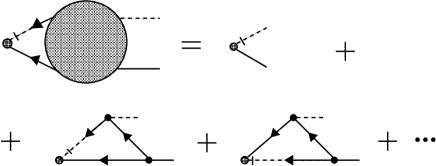
Figure 2: Diagrams needed for calculation the scaling exponent of $\mathcal{O}_{1}$ to 1-loop order.

Our 1-loop calculation, see the diagrams in Fig. 2, yields

$$\Gamma_{\mathcal{O}_{1}}=\lambda f_{1}\left(Z_{11}+\frac{u}{2\varepsilon}+\ldots\right)\mathcal{O}_{1}\,,$$ (27)

where the ellipsis denote terms that are finite for $\varepsilon=6-d\rightarrow 0$. We obtain

$$Z_{11}=1-\frac{u}{2\varepsilon}+O(u^{2})\,.$$ (28)

The renormalization of $\mathcal{O}_{1}$ in detail reads

$$[\mathcal{O}]_{1}=\sum_{\beta}Z_{1\beta}\mathcal{O}_{\beta}=(Z\tilde{Z})^{-1/2}Z_{11}\mathcal{\mathring{O}}_{1}+\ldots\,,$$ (29)

where the ellipsis here denotes the combination of the other $\mathcal{O}_{\beta}$ that is not required for the calculation of the scaling dimension of the attack-ratio. Applying the renormalization-group differential operator

$$\mathcal{D}_{\mu}\cdots:=\left.\mu\frac{\partial\cdots}{\partial\mu}\right|_{0}=\Bigg{(}\mu\frac{\partial}{\partial\mu}+\beta\frac{\partial}{\partial u}+\zeta\lambda\frac{\partial}{\partial\lambda}+\kappa\tau\frac{\partial}{\partial\tau}\Bigg{)}\cdots\,,$$ (30)

to the attack-ratio (the RG-functions $\beta$, $\zeta$, and $\kappa$ can be found in Refs. Ja85 ; JaTa05 ), we get

$$\bigl{(}\mathcal{D}_{\mu}-\omega_{1}\bigr{)}\mathcal{A}_{perc}(\mathbf{x},t,\tau;u,\lambda,\mu)=0\,,$$ (31)

with the exponent $\omega_{1}=\omega_{11}$ at the fixed point $u=u_{\ast}=2\varepsilon/7+O(\varepsilon^{2})$ given by

$$\omega_{1}=\mathcal{D}_{\mu}\ln(Z_{11}/\tilde{Z}^{1/2})=\frac{7}{12}u+O(u^{2})=\frac{\varepsilon}{6}+O(\varepsilon^{2})\,.$$ (32)

Dimensional analysis of $\mathcal{A}_{perc}$ yields

$$\mathcal{A}_{perc}(\mathbf{x},t,\tau;u,\lambda,\mu)=\mu^{d/2}\mathcal{A}_{perc}(\mu\mathbf{x},\lambda\mu^{2}t,\mu^{-2}\tau;u,1,1)\,.$$ (33)

Together with the solution of the RGG (31)

$$\mathcal{A}_{perc}(\mathbf{x},t,\tau;u,\lambda,\mu)=l^{\omega_{1}}\mathcal{A}_{perc}(\mathbf{x},t,l^{\kappa}\tau;u_{\ast},l^{\zeta}\lambda,l\mu)\,,$$ (34)

at the fixed point with $l$ being the dimensionless flow-parameter, we obtain

$$\mathcal{A}_{perc}(\mathbf{x},t,\tau;u,\lambda,\mu)$$

$$=l^{\omega_{1}+d/2}\mathcal{A}_{perc}(l\mathbf{x},l^{z}t,l^{-1/\nu}\tau;u_{\ast},\lambda,\mu)$$

$$=t^{-\alpha_{\mathcal{A}}}F(\mathbf{x}/t^{1/z},\tau t^{1/\nu z})\,,$$ (35)

where $F$ is some scaling function, for the scaling behavior of the attack-ratio. Its scaling exponent is

$$\alpha_{\mathcal{A}}=\Bigg{(}\frac{d}{2}+\omega_{1}\Bigg{)}/z=\frac{3}{2}\Bigg{[}1-\frac{\varepsilon}{36}+O(\varepsilon^{2})\Bigg{]}\,,$$ (36)

where we used the expansion $z=2-\varepsilon/6+O(\varepsilon^{2})$.

Finally, we compare our result to the available numerical data. Currently, we know of such data only for $d=2$, where $\alpha_{\mathcal{A}}=0.518$ Gra2012 . Extrapolating our 1-loop result for $\alpha_{\mathcal{A}}$ as it stands down to $d=2$ is problematic, of course. Thus, we resort to one of the established procedures for improving $\varepsilon$-expansion results, namely rational approximation. The general idea behind this technique is to augment an $\varepsilon$-expansion with higher order terms to incorporate additional information. To this end, we note that in one-dimensional percolation, the attack-ratio is independent of time: microscopically it is simply $1$. Hence, we know rigorously that $\alpha_{\mathcal{A}}=0$ in $d=1$. We incorporate this feature into our result by multiplying the right hand side of Eq. (36) with the factor $\bigl{[}1-(\varepsilon/5)^{2}\bigr{]}$ resulting in the interpolation formula

$$\alpha_{\mathcal{A}}=\frac{3(d-1)}{10}\Bigg{(}1+\frac{31}{180}\varepsilon\Bigg{)}\,.$$ (37)

Note that the extra factor was set up with $\varepsilon$ appearing quadratically and that therefore Eq. (36) and (37) are in absolute agreement to first order in $\varepsilon$ as they should. For $d=2$, our interpolation produces $\alpha_{\mathcal{A}}=0.507$ which is satisfyingly close to the numerical result stated above.

V Concluding Remarks

In summary, we have discussed attacks and infections at percolating fronts based on renormalized dynamical field theory of the EGEP. Important observables measuring these attacks and infections are related to composite operators of this theory that had not been studied hitherto. For the ordinary percolation transition, we calculated the corresponding anomalous exponents to 1-loop order. For the tricritical percolation transition, one has to go at minimum to 2-loop order to get anomalous contributions beyond MF theory. We leave this interesting and challenging problem for future work.

- (1) P. Grassberger private communication, unpublished.
- (2) H.K. Janssen, M. Müller, and O. Stenull, Phys. Rev. E 70, 026114 (2004).
- (3) P. Grassberger, Math. Biosci. 63, 157 (1983).
- (4) D. Mollison, J.R. Stat. Soc. B 39, 283 (1977).
- (5) N.T.J. Bailey, The Mathematical Theory of Infectious Diseases, (Griffin, London, 1975)
- (6) J.D. Murray, Mathematical Biology, (Springer, Berlin 1989).
- (7) H.K. Janssen, Z. Phys. B: Cond. Mat. 58, 311 (1985).
- (8) J.L. Cardy and P. Grassberger, J. Phys. A: Math. Gen. 18, L267 (1985).
- (9) H.K. Janssen and U.C. Täuber, Ann. Phys. (NY) 315, 147 (2005).
- (10) M. Cieplak and M. O. Robbins, Phys. Rev. Lett. 60, 2042 (1988); N. Martys, M. Cieplak, and M. O. Robbins, ibid. 66, 1058 (1991); N. Martys, M. O. Robbins, and M. Cieplak, Phys. Rev. B 44, 12294 (1991); H. Ji and M. O. Robbins, ibid. 46, 14519 (1992); C. S. Nolle, B. Koiller, N. Martys, and M. O. Robbins, Phys. Rev. Lett. 71, 2074 (1993)
- (11) B. Drossel and K. Dahmen, Euro. Phys. J. B 3, 485 (1998).
- (12) G. Bizhani, M. Paczuski, and P. Grassberger, Phys. Rev. E 86, 011128 (2012).
- (13) W. O. Kermack and A. G. McKendrick , Proc. R. Soc. A 115, 700 (1927).
- (14) Note it is not the infected individuals but the disease as a whole that spreads diffusively.
- (15) H.K. Janssen, Z. Phys. B: Cond. Mat. 23, 377 (1976); R. Bausch, H.K. Janssen, and H. Wagner, Z. Phys. B: Cond. Mat. 24, 113 (1976); H.K. Janssen, in Dynamical Critical Phenomena and Related Topics (Lecture Notes in Physics, Vol. 104), edited by C.P. Enz, (Springer, Heidelberg, 1979).
- (16) C. De Dominicis, J. Phys. (France) Colloq. 37, C247 (1976); C. De Dominicis and L. Peliti, Phys. Rev. B 18, 353 (1978).
- (17) H.K. Janssen, in From Phase Transitions to Chaos, edited by G. Györgyi, I. Kondor, L. Sasvári, and T. Tél, (World Scientific, Singapore, 1992).
- (18) U. C. Täuber, Critical Dynamics - A Field Theory Approach to Equilibrium and Non-Equilibrium Scaling Behavior (Cambridge: Cambridge University Press, 2014).
- (19) M. Doi, J. Phys. A 9, 1465, 1479 (1976).
- (20) P. Grassberger and P. Scheunert, Fortschr. Phys. 28, 547 (1980).
- (21) L. Peliti, J. Phys. (France) 46, 1469 (1985).
- (22) J. Cardy, in: Proceedings of Mathematical Beauty of Physics, ed. J.-B. Zuber, Adv. Ser. in Math. Phys. 24, 113 (1997).
- (23) J. Cardy, in: Non-equilibrium Statistical Mechanics and Turbulence, London Math. Soc. Lecture Note Ser. 355, Cambridge University Press, 108 (2008).
- (24) For a critical discussion, which also concerns the appearance of the ‘diffusion noise’ term , see U.C. Täuber, M. Howard, and B.P Vollmayr-Lee, J. Phys. A 38 R79 (2005).
- (25) K.J. Wiese, Phys. Rev. E 93, 042117 (2016).
- (26) O. Stenull and H.K. Janssen, Europhys. Lett. 51, 539 (2000).