Covariations in ecological scaling laws fostered by
community dynamics

Abstract

Scaling laws in ecology, intended both as functional relationships among ecologically-relevant quantities and the probability distributions that characterize their occurrence, have long attracted the interest of empiricists and theoreticians. Empirical evidence exists of power laws associated with the number of species inhabiting an ecosystem, their abundances and traits. Although their functional form appears to be ubiquitous, empirical scaling exponents vary with ecosystem type and resource supply rate. The idea that ecological scaling laws are linked had been entertained before, but the full extent of macroecological pattern covariations, the role of the constraints imposed by finite resource supply and a comprehensive empirical verification are still unexplored. Here, we propose a theoretical scaling framework that predicts the linkages of several macroecological patterns related to species’ abundances and body sizes. We show that such framework is consistent with the stationary state statistics of a broad class of resource-limited community dynamics models, regardless of parametrization and model assumptions. We verify predicted theoretical covariations by contrasting empirical data and provide testable hypotheses for yet unexplored patterns. We thus place the observed variability of ecological scaling exponents into a coherent statistical framework where patterns in ecology embed constrained fluctuations.

A prototypical example of ecological scaling law is the species-area relationship (SAR) on which island biogeography is based [1]. It states that the number of species $S$ inhabiting disjoint ecosystems increases as a power of their area, i.e. $S\propto A^{z}$, where $z$ is the SAR scaling exponent. The widespread interest in scaling laws [2, 3, 4, 5, 6, 7, 8] lies in their intrinsic predictive power, e.g. the use of SAR to forecast how many species might go extinct if the available habitat shrinks or is fragmented into smaller unconnected parts. Precise estimates of the scaling exponents’ values are thus crucial. Empirical evidence, however, shows that they vary considerably across ecosystems [9, 10, 11], suggesting that exponents of scaling ecological laws are far from universal, although the power-law form proves remarkably robust (Fig. 1).

Scaling patterns in ecology have mostly been studied within independent ecosystems, leading to canonical estimates of scaling exponents which may not be simultaneously achievable in a single ecosystem due to extant and consistency constraints. Although ecological scaling laws have historically been treated as disconnected, it is instructive to show by a simple example that they are functionally related. Consider a community hosted within a resource-limited ecosystem of area $A$ whose $i$-th species is characterized by abundance $n_{i}$ and typical body mass $m_{i}$. Empirical evidence suggests that the following patterns can be described at least approximately by power laws, disregarding possible cutoffs at large sizes: i) the community size spectrum [12, 9, 13, 7], $s(m)\propto m^{-\eta}$, i.e., the fraction of individuals of body mass $m$ regardless of species; ii) the distribution of species’ typical body masses [14, 5] $P(m)\propto m^{-\delta}$ and iii) the average abundance of a species with typical body mass $m$, $\langle n|m\rangle\propto m^{-\gamma}$ (Damuth’s law [3, 15] or local size-density relationship [7]). A back-of-the-envelope calculation suggests that the total number of individuals of mass $m$ (regardless of species) is the product of the number of species with typical mass $m$ and the average abundance of a species with typical mass $m$ (i.e., $s(m)\propto P(m)\langle n|m,A\rangle$). Thus, the scaling exponents must satisfy the consistency relationship:

$$\eta=\delta+\gamma,$$ (1)

which proves that exponents measured in the same ecosystem are not independent, unlike exponents measured in disparate ones. This example and a few others identified in earlier works [13, 16, 17, 18] and in the context of MaxEnt [19] highlight the need for a framework that comprehensively accounts for linking relationships among macroecological scaling laws.

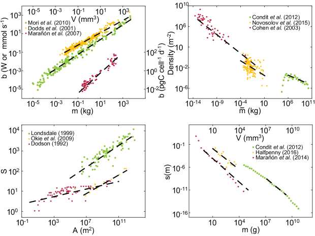
Figure 1: Empirical evidence of scaling ecological patterns in different ecosystems: forests (green), terrestrial (yellow) and aquatic ecosystems (magenta). Regression lines are linear least square fits of log-transformed data. A) Kleiber’s law: metabolic rates in $\mu$mol $s^{-1}$ (forests), W (terrestrial ecosystems), pgC cell^-1 d^-1 (aquatic ecosystems). Size in kg (forests and terrestrial ecosystems) and in $\mu$m³ (aquatic ecosystems); B) Damuth’s Law ($\bar{m}$ is a species’ mean mass); C) SAR; D) Community size-spectrum: size in g (forests and terrestrial ecosystems) and $\mu$m³ (aquatic ecosystems). See SI (section 2) for scaling exponents estimates/errors. References to the datasets are provided in Table S2.

Results

Here, we show that supply limitation imposes precise constraints on macroecological patterns, along with consistency relationships such as (1). Assuming that individual resource consumption (metabolic) rates under field conditions, $b$, relate to body mass $m$ via Kleiber’s law [2, 20, 21], i.e. $b=cm^{\alpha}$ (with $\alpha\leq 1$, $c$ constant), we argue that the constraint placed on the total community consumption rate $B$ by the finiteness of available resources translates into constraints on sustainable body sizes and abundances. To show this, we move from a scaling ansatz for the joint probability $P(n,m|A)dndm$ of finding a species of abundance $n\in[n,n+dn]$ and typical mass $m\in[m,m+dm]$ within an ecosystem of area $A$, that postulates correlated fluctuations in mass and abundance for any species. Such joint distribution, which we term the ‘fundamental distribution’, must be viable in the sense that its marginals must reproduce the empirical scaling observed in the field. Our conclusion (Methods, SI) is that a general, yet analytically tractable to some extent, form for $P(n,m|A)$ is:

$$P(n,m|A)=(\delta-1)m^{-\delta}n^{-1}G\Bigl{(}\frac{n}{\langle n|m,A\rangle}\Bigr{)}$$ (2)

where:

$$P(m|A)=(\delta-1)m^{-\delta}$$ (3)

is the probability density of finding a species of typical mass $m\in[m,m+dm]$,

$$P(n|m,A)=n^{-1}G\Bigl{(}\frac{n}{\langle n|m,A\rangle}\Bigr{)}$$ (4)

is the probability density of finding a species of abundance $n\in[n,n+dn]$ among those of mass $m$ and

$$\langle n|m,A\rangle=m^{-\gamma}A^{\Phi}h\left(\frac{m}{A^{\lambda}}\right)$$ (5)

is the average abundance of a species of typical mass $m$ within an ecosystem of area $A$. The properties of $G$ and $h$ are described in the Methods and in the SI (section 1.3).

Eqs. (2–5), through their marginals and moments, give rise to the empirically-observed set of macroecological scaling laws (SI section 1), namely: the SAR, $S\propto A^{z}$; Damuth’s law, $\langle n|m,A\rangle\propto A^{\Phi}m^{-\gamma}$, where the $A$ dependency is an addition to the original relationship proposed by Damuth; the community size-spectrum $s(m|A)\propto m^{-\eta}$; the species’ mass distribution $P(m|A)\propto m^{-\delta}$; the scaling of the total biomass, $M\propto A^{\mu}$; the scaling of the total abundance [22], $N\propto A^{\nu}$; the scaling of the largest organism’s mass [23, 8], $m_{\max}\propto A^{\xi}$; the relative species’ abundance (RSA) [24], defined as the probability of finding a species with abundance $n$; Taylor’s law [25, 26], linking mean and variance of a species’ abundance as $\langle n^{2}\rangle-\langle n\rangle^{2}\propto\langle n\rangle^{\beta}$. Note that the SAR and the scaling of $N$ and $M$ with $A$ are predictions (i.e., not assumptions) of our framework which follow from the imposed constraint on shared resources.

In addition to Eq. 1, the scaling framework predicts the following exact relationships among scaling exponents:

$$z=1-\Phi-\max\{0,\lambda(1+\alpha-\eta)\}$$ (6)

$$\mu=1+\max\{0,\lambda(2-\eta)\}-\max\{0,\lambda(1+\alpha-\eta)\}$$ (7)

$$\nu=1-\max\{0,\lambda(1+\alpha-\eta)\}$$ (8)

$$\xi=\frac{z}{\delta-1}$$ (9)

where $\lambda$ accounts for a finite-size effect in Damuth’s law: $\langle n|m,A\rangle=A^{\Phi}m^{-\gamma}h(m/A^{\lambda})$, with $\lim_{x\to 0}h(x)=\mbox{const}$ and $\lim_{x\to\infty}h(x)=0$ (Methods). The exponent $\beta$ does not appear because its value is found to be independent from other exponents [26] (Methods). Only $5$ of the $10$ observable exponents are thus independent. (6) implies, in any ecosystem where $z>0$, as observed for forests [27], mammals [8] and lizards [28], that $\Phi<1$ and therefore species’ densities decrease with increasing area. (9) is compatible with the linking relationship derived in Southwood et al. [16], which is shown here to be one component of a broader set of linking relationships (SI section 1.9). Also, area-independent constraints to the maximum size of an organism may lead to a breakdown of Eq. 9 at large $A$ (SI, section 1.8.3).

To corroborate the validity of our framework, we investigated a broad class of stochastic models for the dynamics of a community limited by resource supply which is assumed to be proportional to the ecosystem area (Methods and SI section 3). Despite major changes in the speciation dynamics and regardless of parametrization, all models are compatible with the finite-size scaling structure of $P(n,m|A)$ and therefore reproduce both the macroecological laws reported above and their covariations.

The empirical verification of all the relationships (1, 6–9) would require the simultaneous measurement within the same ecosystem of all scaling exponents. Unfortunately, such a comprehensive dataset does not seem to exist to date. Therefore, we searched for empirical data that would allow verifying, at least partially, Eqs. (1,6–9). We found that (1) is verified within the errors in the tropical forests datasets of Barro Colorado Island (BCI, see Fig. 2) [29] and of the Luquillo forest [30] (Methods and SI section 2.2.1). (6) is verified within the errors in a dataset of lizard population densities on 64 islands worldwide (LIZ) [28] (SI section 2.2.2). Finally, (9) is verified within one standard error in a dataset of mammal body sizes in several islands in Sunda Shelf (SSI) [8] (Methods and SI section 2.2.3). All the empirical tests performed are summarized in table S11.

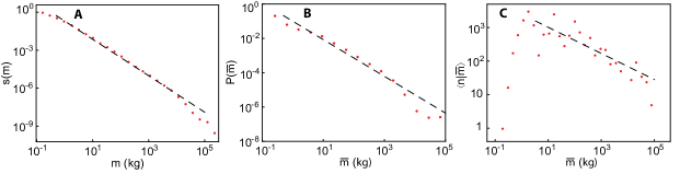
Figure 2: Empirical evidence of scaling patterns in Barro Colorado Island [29], seventh census: A) Community size-spectrum, i.e. the probability distribution of individuals’ mass regardless of species (red dots), B) Distribution of species mean masses $P(\bar{m})$ (red dots), C) Damuth’s law, i.e. the average abundance $\langle n|\bar{m},A\rangle$ of a species of mean mass $\bar{m}$ (red dots), where each point is the average abundance over bins of logarithmic size. Dashed black lines show power-functions with exponents as in Table S3. Details on exponents’ estimates are reported in the Methods and SI (section 2.2.1).

Discussion

The theoretical framework proposed here rationalizes the observed variability of ecological exponents across ecosystems. Jointly with empirical evidence, our framework supports the tenet that scaling exponents may vary across ecosystems but must satisfy consistency relationships that result in exact covariations of ecological patterns. When applying scaling laws, for example in conservation, care should be exerted not to combine exponents measured in different settings, which may not satisfy the relationships (1, 6–9) leading to misled predictions for unmeasured patterns.

Our framework adopts the minimum set of hypotheses allowing to reproduce widespread macroecological patterns found in empirical data, without compromising analytical tractability. Such analytical tractability is important in this context because it highlighs the relationships among macroecological patterns in simple terms, i.e. via algebraic relationships among their scaling exponents. However, there may be empirical examples where some of the patterns considered here deviate from pure power-laws. The framework presented here already comprises cut-offs in the community size-spectrum and in Damuth’s law, allowing deviation from pure power-law behavior at large body sizes, and can be generalized to describe more complex ecological settings. For example, one can account for the fact that individuals’ body sizes within the same species are characterized by intra-specific distributions [31]. Such generalization of the framework bears no modification to the linking relationships among macroecological laws, unless intra-specific size-distribution are heavy-tailed, in which case corrections apply (SI section 1.8.4 and 1.8.5). One can also account for curvatures in Kleiber’s law [32, 33, 34, 35], which are found to induce curvatures in the species-area relationship (SI section 1.8.1). A cut-off or a non-power-law form for $P(m|A)$ can also be considered (SI section 1.8.6). Finally, the assumption that all individuals share the same resources would imply that our results apply to single trophic levels. However, we show in the SI (section 1.8.2) how our framework can be extended to describe multi-trophic systems. In the most general scenario in which the dependence of $P(m|A)$ on $m$ and $\langle n|m,A\rangle$ on $m$ and $A$ cannot be expressed as in (3) and (5) (which, however, are compatible with several empirical case studies) nor described by the generalizations treated in the SI section 1.8.6, one would have to rely on numerical methods to derive the covariations between macroecological patterns, following the same route adopted in our theoretical investigation. We anticipate that generalizations of Eqs. (1,6–9) would hold in this scenario, although they would be expressed as integral equations in terms of the probability distributions introduced above. The next step in the study of co-varying ecological patterns is the identification of the mechanisms that determine the values of the independent exponents. For example, theoretical evidence [36] suggests that the value of $z$ is affected by topological constraints posed by the ecological substrate.

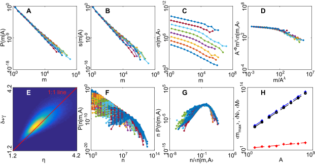
Figure 3: Scaling patterns from the basic community dynamics model (Methods). Different colors refer to different values of $A=10^{i}$, from $i=1$ (lower blue curve in panel C) to $i=8$ (upper blue curve in panel C). Panels A, B, C and f show respectively $P(m|A)$, $s(m|A)$, $\langle n|m,A\rangle$ and $P(n|m,A)$ at stationarity. Panels D and G show collapses of $\langle n|m,A\rangle$ and $P(n|m,A)$. Eqs. (4-5) are verified because the curves $nP(n|m,A)$ versus $n/\langle n|m,A\rangle$ collapse on the same curve for different $A$ (panel G), and so do the curves $m^{\gamma}A^{-\Phi}\langle n|m,A\rangle$ versus $m/A^{\lambda}$ (panel D). Panel E: density histogram plot of $\eta$ vs $\delta+\gamma$ at different times. Panel H: scaling of $\langle m_{\max}\rangle$ (red crosses and dashed lines), $\langle N\rangle$ (black dots and dashed lines) and $\langle M\rangle$ vs $A$ (blue crosses and dashed lines).

Methods

The fundamental distribution $P(n,m|A)$

We consider an ecosystem of area $A$. We assume that the minimum viable mass for an organism is $m_{0}>0$ independent of $A$, so that $P(n,m|A)$ is zero for $m<m_{0}$. We measure mass and area in units of $m_{0}$ and of a reference unit area $a_{0}$, so that $m$ and $A$ are dimensionless. To comply with empirical evidence [14, 5], we assume that $P(m|A)$ is a power function of $m$ (Eq. 3): $P(m|A)=(\delta-1)m^{-\delta}$, where $\delta>1$ ensures integrability (see also the SI (section 1.8.6)). For $P(n|m,A)$, in accordance with the community dynamics models and with the empirical observation of Damuth’s law, we posit (Eq. 4): $P(n|m,A)=n^{-1}G\left(n/{\langle n|m,A\rangle}\right)$, where $G(x)$ is such that $\int_{0}^{\infty}x^{j}G(x)dx<\infty$ for $j=-1,0,1$ and (Eq. 5) $\langle n|m,A\rangle=m^{-\gamma}A^{\Phi}h({m}/{A^{\lambda}})$ is the average abundance of a species of typical mass $m$ in an ecosystem of area $A$. The properties of $G$ ensure that $\int_{0}^{\infty}dn\ n\ P(n|m,A)=\langle n|m,A\rangle$, that is, Damuth’s law is reproduced. The factor $n^{-1}$ in (4) is discussed in the SI. The function $h(x)$ describes an $A$-dependent cutoff on the abundances as observed in simulations of stochastic models of community dynamics (see, e.g., Fig. 3C). $h(x)$ is such that $h(x)=o\left(x^{-2+\delta+\gamma}\right)$ as $x\to\infty$ to ensure convergence of the moments we are interested in and $\lim_{x\rightarrow 0}h(x)=h_{0}$ constant to yield a power law regime before the cut-off. Eqs. (2–5) constitute our ansatz on the scaling form of $P(n,m|A)$.

Derivation of scaling ecological laws

Eq. (2) can be used to compute the scaling of the ($j$,$k$)-th moment with $A$ exactly (see SI section 1.6 for the detailed computation) as:

$$\begin{split}I_{j,k}&=\int_{1}^{\infty}\int_{0}^{\infty}n^{j}m^{k}P(n,m|A)dndm\\ &\propto A^{j\Phi+\max\{0,\lambda(1+k-\delta-j\gamma)\}}.\end{split}$$ (10)

Scaling laws are derived from Eq. 10 as follows:

i) Species-Area Relationship. The total number of species $S$ is linked to the area $A$ via the constraint $B\propto A$ (SI sections 1.1 and 1.2). The total metabolic rate of the community is:

$$B\propto S\ I_{1,\alpha}=S\int_{1}^{\infty}\int_{0}^{\infty}nm^{\alpha}P(n,m|A)dndm.$$ (11)

where we have used Kleiber’s law. The hypothesis $B\propto A$ (SI sections 1.1 and 1.2) leads to:

$$S\propto A^{z},\mbox{ with }z=1-\Phi-\max\{0,\lambda(1+\alpha-\delta-\gamma)\},$$ (12)

which corresponds to Eq. 6. Note that, if $z>0$, this equation predicts that species’ densities decrease with increasing $A$ (recall that $\langle n|m,A\rangle\propto A^{\Phi}$ with $\Phi<1$). This can be understood through a heuristic argument: if $N\propto A^{\nu}$ with $\nu\leq 1$ and $S\propto A^{z}$, it follows that the average abundance per species scales sub-linearly as $\langle n|A\rangle=N/S\propto A^{\nu-z}$. Such scaling of $\langle n|A\rangle$ with $A$ is retained by the average abundance conditional on body size, $\langle n|m,A\rangle$, and thus back-of-the-envelope calculations suggest $\Phi=\nu-z$, which coincides with Eq. 6 and (12), given Eq. 8. This result is a novel prediction of our framework and implies that species’ densities decrease with ecosystem area. Note also that we refer here to the so-called island SAR [37], obtained by counting species inhabiting disjoint patches of land (e.g. islands, lakes or, in general, areas separated by environmental barriers from the surroundings which we can think of as closed ecosystems) rather than to nested SARs where areas are sub-patches of a single larger domain [38, 39]. The two SARs are quite different, as the nested SAR is related to the spatial distribution of individuals, while the island SAR stems from complex eco-evolutionary dynamics shaping the community;

ii) Damuth’s law is traditionally intended as the scaling of the average density of a species, ${\langle n|m,A\rangle}/{A}$, with its typical mass $m$. However, as discussed in i), the density of a species depends on the inhabited area, as found for example in our empirical analyses of the LIZ dataset [28] (see SI section 2.2.4). Thus, we consider here a generalized version of Damuth’s law, relating the average abundance $\langle n|m,A\rangle$ to the typical mass of the species and to the area of the ecosystem $A$. Indeed, in our framework the average abundance of a species of characteristic mass $m$ in an ecosystem of area $A$ is:

$$\begin{split}\langle n|m,A\rangle&=\int_{0}^{\infty}nP(n|m,A)dn\\ &=\int_{0}^{\infty}G\left[\frac{nm^{\gamma}}{A^{\Phi}}\frac{1}{h\left({m}/{A^{\lambda}}\right)}\right]dn\\ &=A^{\Phi}m^{-\gamma}h\left(\frac{m}{A^{\lambda}}\right)\int_{0}^{\infty}G\left(x\right)dx\\ &\propto A^{\Phi}m^{-\gamma}h\left(\frac{m}{A^{\lambda}}\right),\end{split}$$ (13)

where the properties of $G$ ensure the convergence of the integral. The average abundance of a species of mass $m$, thus, has a power-law dependence on $m$ and $A$, as found in empirical data, and an $A$-dependent cutoff at large masses provided by the function $h$, as shown by our community dynamics models (Fig. 3C).

iii) Scaling of total biomass. The total biomass can be computed as:

$$\begin{split}M&=S\langle nm\rangle=S\ I_{11}\\ &\propto A^{1+\max\{0,\lambda(2-\delta-\gamma)\}-\max\{0,\lambda(1+\alpha-\delta-\gamma)\}},\end{split}$$ (14)

yielding Eq. 7 of the main text.

iv) Scaling of total number of individuals. The total number of individuals $N$ in the ecosystem is given by:

$$N=S\langle n\rangle=S\ I_{10}\propto A^{1-\max\{0,\lambda(1+\alpha-\delta-\gamma)\}},$$ (15)

yielding Eq. 8 of the main text.

v) Community size-spectrum. The size spectrum $s(m|A)$ is the probability that a randomly sampled individual (regardless of its species) has mass in $[m,m+dm]$ and is therefore equal to:

$$\begin{split}s(m|A)&=\frac{S}{N}\int_{0}^{\infty}nP(n,m|A)\ dn\\ &\propto A^{-\max\{0,\lambda(1-\delta-\gamma)\}}m^{-\delta-\gamma}h\left(\frac{m}{A^{\lambda}}\right)\\ &=m^{-\delta-\gamma}h\left(\frac{m}{A^{\lambda}}\right),\end{split}$$ (16)

where we have used (12) and (15), $\delta>1$ and the properties of $G$ ensure the convergence of the integral. The size spectrum has a power-law dependence on $m$ and we can identify $\eta=\gamma+\delta$, corresponding to Eq. 1. Furthermore, $s(m|A)$ displays a cutoff at $m\propto A^{\lambda}$.

vi) Scaling of the maximum body mass. The maximum body mass observed in an ecosystem is $m_{\max}$ such that $S\int_{m_{\max}}^{\infty}P(m|A)dm=1$, that is, the maximum mass extracted in $S$ samples drawn from $P(m|A)$ (see also the discussion in the SI section 1.9). Substituting $S\propto A^{z}$ we find $\int_{m_{\max}}^{\infty}x^{-\delta}dx\propto A^{-z}$, leading to:

$$m_{\max}\propto A^{\frac{z}{\delta-1}},$$ (17)

which implies $z=\xi(\delta-1)$, i.e. Eq. 9.

vii) Taylor’s law. Its exponent is given by:

$$\beta=\frac{\log\langle n^{2}\rangle_{m}}{\log\langle n\rangle_{m}}=2+O\left(\frac{1}{\log(A)}\right).$$ (18)

In the large area limit $\beta=2$ which is the value typically found empirically [26]. Note that this computation of Taylor’s law corresponds to the so-called ‘spatial Taylor’s law’ and not to its temporal counterpart [26], in which case empirical estimates typically report values of $\beta\in[1,2]$. Deviations from $\beta=2$ may arise from the logarithmic correction in Eq. 18 and from the fact that the scaling of the variance (which is the second cumulant) and the second moment may differ [26].

viii) Relative Species Abundance. It is the distribution of species’ abundances:

$$P(n|A)=\int_{1}^{\infty}\ P(n,m|A)dm.$$ (19)

There has been much interest in its analytical form. In our theoretical framework, $P_{RSA}$ cannot be computed in the general case where the exact form of $h$ and $G$ is unknown. SI (section 1.7) reports an approximate analytical computation for a particular choice of the two functions satisfying the required properties, yielding a RSA with a tail well approximated by a lognormal.

Data analysis

Equation 1. We verified Eq. 1 on censuses of Barro Colorado Island (BCI) [29, 40, 41] (Fig. 2) and of the Luquillo forest [30] (Fig. S4). Tree diameters were converted into mass using an established allometric relationship between mass and diameter [42, 43], $m\propto d^{8/3}$. For each species, we used the mean mass of its individuals as our estimate of the typical species’ mass $\bar{m}$. To account for possible deviations from the power-law behavior at small and large values of $\bar{m}$ we performed a maximum-likelihood estimation (SI section 2.2.1) of $\delta$ and $\eta$ by considering only the species with mass larger than a lower cutoff and by accounting for possible finite-size effects at large $\bar{m}$ in the form of a cut-off function (SI section 2.2.1). The estimation of the exponent $\gamma$ of Damuth’s law in tropical forest datasets is affected by the sampling protocol and a correction is required to avoid sampling bias (SI section 2.2.1). In our analysis, we used the fifth, sixth and seventh censuses of BCI and the five censuses of the Luquillo forest available online in the Center for Tropical Forest Science dataset collection. All censuses satisfy the relationship (1) within the errors. Whereas BCI censuses appear very similar to each other (and therefore also the exponent values estimated in different censuses, see Table S3), the Luquillo forest appears to be more dynamic (we note that the forest was hit by a major hurricane between the second and the third censuses), with values of $\gamma$ decreasing in time after $1998$ (second census, see Table S4). Because the estimate of $\delta$ remains constant, our framework would predict via Eq. 1 that $\eta$ would also decrease in time, and this is found to be true. Finally, we note that both the BCI and the Luquillo datasets reject the linking relationship $\eta=\delta$ predicted earlier by a scaling framework [17] which is not capable of reproducing Damuth’s law (Fig. S2).

Equation 6. Eq. 6 is verified within one standard error in a dataset gathering population densities of several species of lizards on 64 islands worldwide (LIZ) [28], with areas ranging from 10^-1 to 10⁵ km², where $\Phi=0.78\pm 0.08$, $z=0.17\pm 0.01$(mean$\pm$SE, $R^{2}=0.46$) and $\max\{0,\lambda(1+\alpha-\eta)\}=0$ because $\alpha\leq 1$ and $\eta=\delta+\gamma=1.98\pm 0.07$ (mean$\pm$SE), see Table S5 and Fig. S8 of the SI. Details of the fitting procedures and further discussion of the results can be found in section SI 2.2.2.

Equation 9. To test the validity of Eq. 9 we used a dataset of mammals species presence/absence data on several islands in Sunda Shelf (SSI) [8], covering more than four orders of magnitude in island areas. The SAR and the scaling of the maximum body mass with the area were fitted by linear least-square regression on log-transformed data, while $P(m|A)$ was fitted by maximum-likelihood [44]. Scaling exponents in this dataset are reported in Table S6. Eq. 9 is verified in the SSI dataset within the errors, with $z=0.23\pm 0.02$ (mean$\pm$SE, $R^{2}=0.93$), $\delta=1.6\pm 0.2$ (mean$\pm$SE) and $\xi=0.49\pm 0.09$ (mean$\pm$SE, $R^{2}=0.76$).

Stochastic models of community dynamics

We developed several community dynamics models accounting for the constraint on resource supply rate and incorporating empirically observed allometric relationships for the dependence of vital rates on individuals’ body sizes [4]. In all our models, the birth and death rates at which an individual of a species of mass $m_{i}$ and abundance $n_{i}$ is born or dies are, respectively:

$$\begin{split}u_{i}&=m_{i}^{-\theta}n_{i},\\ v_{i}&=\left[v_{0}+(1-v_{0})c\frac{\sum_{j}n_{j}m_{j}^{\alpha}}{\mathcal{R}}\right]m_{i}^{-\theta}n_{i},\end{split}$$ (20)

and thus the per-capita growth rate of species $i$ is $\frac{u_{i}-v_{i}}{n_{i}}=(1-v_{0})\left[1-\frac{c}{\mathcal{R}}{\sum_{j}n_{j}m_{j}^{\alpha}}\right]m_{i}^{-\theta}$, which is equal to zero when $c\sum_{j}n_{j}m_{j}^{\alpha}=\mathcal{R}\propto A$, where $\mathcal{R}$ is the resource supply rate. At the stationary state, therefore, the total rate of resource consumption of the community fluctuates around $\mathcal{R}$ but the ecological dynamics continues and determines species’ abundances through the constraints imposed by resources and by physiological rates. Speciation was implemented in several ways (SI section 3), in order to test the robustness of our results to changes in the models’ assumptions. We investigated models where we fixed the total number of species $S\propto A^{z}$ (SI section 3.1) and models where $\langle S\rangle\propto A^{z}$ is an emergent property of the community dynamics (SI section 3.2). By performing data-collapses (Fig. 3) of $P(m|A)$, $P(n|m,A)$ and $\langle n|m,A\rangle$ calculated using model data, we verified that they all comply with Eqs. (2–5). We note that the scaling exponents in Eqs. (1,6–9) depend on model specifications, but the scaling properties of the fundamental distribution $P(n,m|A)$ specified in Eqs. (2–5) always hold.

Basic community dynamics model

In this section we describe the simplest model of community dynamics that reproduces the set of empirically-observed macroecological laws reported in the main text. We shall refer to such model as the basic model. Variations of the basic model assumptions, the exploration of parameters’ space and other models are discussed in the SI (section 3).

In the basic model, each species speciates with probability $w$ per unit time (i.e., species-specific speciation events are Poisson-distributed with rate $w$). At each speciation event, a species is selected at random and a random fraction of individuals from such species is assigned to a new species $j$. The mass of the new species is obtained from the mass of the parent species as $m_{j}=\max\{m_{0};qm_{i}\}$ where $q$ is extracted from a lognormal distribution with mean and variance equal to unity so that the descendant has, on average, the same mass of the parent species. The maximum in the expression for $m_{j}$ ensures that the bound on the minimum mass $m_{0}$ that a species can attain is satisfied. The mass of the parent species is left unchanged. Species’ masses thus undergo a process that is a combination of a multiplicative bounded process, known to produce power-laws [45, 46], and of the birth/death dynamics.

The number of species $S$ is set to a constant value proportional to the area: $S=10A^{z}$. Although the number of species in natural ecosystems may fluctuate in time, fixing it in the basic model allows us to vary the scaling exponent $z$ to effectively account for relevant ecological and evolutionary processes not included in the model which may affect the value of $z$ in natural ecosystems (SI, section 3.4). Note that fixing the number of entities in the model (here, $S$) is a common approximation in many related fields, such as population genetics (e.g., the Wright-Fisher model [47] with fixed population size $N$) and neutral and metacommunity theory [39]. To maintain $S$ constant, we imposed that each extinction event causes a speciation event. Viceversa, at each speciation event, extinction is enforced on a species selected at random with probability inversely proportional to its abundance (i.e., more abundant species are less likely to go extinct) and proportional to the power $-\theta$ of its mass, which accounts for the fact that ecological rates are faster for smaller species. A variation on this extinction rule is discussed in the SI (section 3.1.2). Models where $\langle S\rangle\propto A^{z}$ is an emergent random variable are discussed in the SI (section 3.2).

The total number of individuals $N=\sum_{i=1}^{S}n_{i}$ and the total biomass $M=\sum_{i=1}^{S}n_{i}m_{i}$ are not fixed in the basic model (nor in the other models discussed in the SI section 3), but fluctuate in time around mean values that depend on the models’ parameters and, most importantly, on the ecosystem area $A$. In other words, the mean biomass and the mean total abundance are given by a balance between birth, death and speciation events, with the constraint of resource supply limitation set by the ecosystem area $A$. The model thus allows to study the scaling of the total number of individuals and the total biomass as functions of $A$.

The distribution $P(m|A)$ exhibits power-law behavior in $m$ ((3)) (Fig. 3A). The size spectrum is also a power-law across several orders of magnitude (Fig. 3B). The curves $\langle n|m,A\rangle$ exhibit power-law behavior in $m$ and $A$ with a cutoff at large $m$ (Fig. 3C). Data collapse (Fig. 3D) shows that its functional form is the one given by Eq. 5. In fact, the curves $m^{\gamma}A^{-\Phi}\langle n|m,A\rangle$ plotted versus $m/A^{\lambda}$ collapse onto the same curve for different values of $A$. Moreover, Fig. 3F shows that the curves $nP(n|m,A)$ versus $n/\langle n|m,A\rangle$ collapse onto the same curve for different values of $m$ and $A$, implying that Eq. 4 holds. The mean total biomass $\langle M\rangle$, the mean total abundance $\langle N\rangle$ and the mean maximum mass $\langle m_{\max}\rangle$ were measured for each value of $A$ as the means across sampling times and are power functions of $A$. Parameter values used to generate the simulation data reported in Fig. 3 are reported in the SI, section 3.1.1. The stochastic model was simulated via a Gillespie tau-leap algorithm with estimated midpoint technique [48], with time step $\tau=1$.

Because the ansatz for the fundamental distribution $P(n,m|A)$ given by Eqs. (2–5) holds, the linking relationships among exponents (Eqs. 1,6–9) are satisfied at steady state by the basic model and by the other models studied in the SI (section 3). The linking relationship $\eta=\delta+\gamma$ is satisfied by the mean values of the exponents, and the density scatter-plot computed counting the occurrences of the pairs $(\eta,\delta+\gamma)$ during the temporal evolution of the community dynamics model (Fig. 3E, shown are simulation data for the largest area value) is peaked along the 1:1 line. Thus, Eq. 1 is satisfied, on average, during the temporal evolution of the community dynamics model.

A broad range of empirical evidence (see SI section 2) shows that ecological patterns are compatible with the predictions of our framework, which also agrees with heuristic calculations as shown in the main text and above. Thus, we hypothesize that our scaling framework describes not only the basic community dynamics model described here and the models described in the SI (section 3), but more generally any ecosystem subject to the constraint of finite resource supply rate. Further discussions on the specificity of our community dynamics models and the generality of our scaling framework are provided in the SI (sections 3.3 and 3.4). The basic model is thus arguably the simplest of a class of models that share the same scaling properties of the fundamental distribution, which in turn imply the same covariations of ecological patterns. This is akin to the concept of universality class [49, 50], applied to the scaling form rather than to the exponents of the joint probability distribution and of ecological scaling laws.

References

- [1] MacArthur RH, Wilson EO (1963) An equilibrium theory of insular zoogeography. Evolution 17, 373–387.
- [2] Kleiber M (1932) Body size and metabolism. Hilgardia 6, 315–353.
- [3] Damuth J (1981) Population density and body size in mammals. Nature 290, 699–700.
- [4] Brown JH, Gillooly JF, Allen AP, Savage VM, West GB (2004) Toward a metabolic theory of ecology. Ecology 85, 1771–1789.
- [5] Marquet PA, et al. (2005) Scaling and power-laws in ecological systems. J. Exp. Biol. 208, 1749–1769.
- [6] Solé R, Bascompte J (2006) Self-Organization in Complex Ecosystems (Princeton University Press, Princeton).
- [7] White EP, Ernest SKM, Kerkhoff AJ, Enquist BJ (2007) Relationships between body size and abundance in ecology. Trends Ecol. Evol. 22, 323–330.
- [8] Okie JG, Brown JH (2009) Niches, body sizes, and the disassembly of mammal communities on the Sunda Shelf islands. Proc. Natl Acad. Sci. USA 106 (2), 19679–19684.
- [9] Cavender-Bares KK, Rinaldo A, Chisholm SW (2001) Microbial size spectra from natural and nutrient enriched ecosystems. Limnol. Oceanogr. 46, 778–789.
- [10] Finkel ZV, Irwin AJ, Schofield O (2004) Resource limitation alters the 3/4 size scaling of metabolic rates in phytoplankton. Marine Ecology Progress Series 273, 269–279.
- [11] Marañón E (2015) Cell Size as a Key Determinant of Phytoplankton Metabolism and Community Structure. Ann. Rev. Marine Science 7, 241–264.
- [12] Sheldon RW, Prakash A, Sutcliffe H (1972) The size distribution of particles in the ocean. Limnol. Oceanogr. 17, 327–340.
- [13] Rinaldo A, Maritan A, Cavender-Bares KK, Chisholm SW (2002) Cross-scale ecological dynamics and microbial size spectra in marine ecosystems. P. Roy. Soc. B: Bio 269, 2051–2059.
- [14] Marquet PA, Taper ML (1998) On size and area: Patterns of mammalian body size extremes across landmasses. Evol. Ecol. 12, 127–139.
- [15] Marquet PA, Navarrete SA, Castilla JC (1990) Scaling Population Density to Body Size in Rocky Intertidal Communities. Science 250, 1125–1127
- [16] Southwood TRE, May RM, Sugihara G (2006) Observations on related ecological exponents. Proc. Natl Acad. Sci. USA 103, 6931–6933.
- [17] Banavar JR, Damuth J, Maritan A, Rinaldo A (2007) Scaling in ecosystems and the linkage of macroecological laws. Phys. Rev. Lett. 98, 068104.
- [18] Grilli J, Bassetti B, Maslov S, Cosentino Lagomarsino M (2012) Joint scaling laws in functional and evolutionary categories in prokaryotic genomes. Nucleic Acids Res. 40, 530–540.
- [19] Harte J (2011) Maximum Entropy and Ecology. A Theory of Abundance, Distribution, and Energetics. (Oxford Univ Press, Oxford).
- [20] West GB, Brown JH, Enquist BJ (1997) A General Model for the Origin of Allometric Scaling Laws in Biology. Science 276, 122–126.
- [21] Banavar JR, Maritan A, Rinaldo A (1999) Size and form in efficient transportation networks. Nature 399, 130–132.
- [22] Hubbell SP (2001) The Unified Neutral Theory of Biodiversity and Biogeography (MPB-32) (Princeton Univ Press, Princeton)
- [23] Burness GP, Diamond J, Flannery T (2001) Dinosaurs, dragons, and dwarfs: the evolution of maximal body size. Proc. Natl Acad. Sci. USA 98, 14518–14523.
- [24] Preston FW (1948) The Commonness, And Rarity, of Species. Ecology 29, 254–283.
- [25] Cohen JE, Xu M, Schuster WSF (2012) Allometric scaling of population variance with mean body size is predicted from Taylor’s law and density-mass allometry. Proc. Natl Acad. Sci. USA 109, 15829–15834.
- [26] Giometto A, Formentin M, Rinaldo A, Cohen JE, Maritan A (2015) Sample and population exponents of generalized Taylor’s law. Proc. Natl. Acad. Sci. USA 112, 7755–7760.
- [27] Lonsdale WM (1999) Global Patterns of Plants Invasions and the Concept of Invasibility. Ecology 80, 1522–1536.
- [28] Novosolov M, Rodda GH, Feldman A, Kadison AE, Dor R, Meiri S (2015) Power in numbers. The evolutionary drivers of high population density in insular lizards. Global Ecol. Biogeogr. 25, 87–95.
- [29] Condit R, Lao S, Pérez R, Dolins SB, Foster R, Hubbell S (2012) Barro Colorado Forest Census Plot Data (Version 2012).
- [30] Zimmerman JK, Comita LS, Thompson J, Uriarte M, Brokaw N (2010) Patch dynamics and community metastability of a subtropical forest: compound effects of natural disturbance and human land use. Landscape Ecology 25, 1099–1111.
- [31] Giometto A, Altermatt F, Carrara F, Maritan A, Rinaldo A (2013) Scaling body size fluctuations. Proc. Natl Acad. Sci. USA 110, 4646–4650.
- [32] Kolokotrones T, Savage V, Deeds EJ, Fontana W (2010) Curvature in metabolic scaling. Nature 464, 753–756.
- [33] Mori S, et al. (2010) Mixed-power scaling of whole-plant respiration from seedlings to giant trees. Proc. Natl Acad. Sci. USA 107, 1447–1451.
- [34] Marañón E, et al. (2013) Unimodal size scaling of phytoplankton growth and the size dependence of nutrient uptake and use. Ecol. Lett. 16, 371–379.
- [35] Banavar JR, Cooke TJ, Rinaldo A, Maritan A (2014) Form, function, and evolution of living organisms. Proc. Natl Acad. Sci. USA 111, 3332–7.
- [36] Bertuzzo E, et al. (2011) Spatial effects on species persistence and implications for biodiversity. Proc. Natl Acad. Sci. USA 108, 4346–4351.
- [37] Preston FW (1962) The Canonical Distribution of Commonness and Rarity: Part I. Ecology 43, 185–215.
- [38] Harte J, Smith AB, Storch D (2009) Biodiversity scales from plots to biomes with a universal species-area curve. Ecol. Lett. 12, 789–797.
- [39] Azaele S, et al. (2016) Statistical mechanics of ecological systems: neutral theory and beyond. Rev. Mod. Phys. 88, 035003.
- [40] Condit R (1998) Tropical Forest Census Plots. (Springer-Verlag and R. G. Landes Company, Berlin, Germany, and Georgetown, Texas).
- [41] Hubbell SP, et al. (1999) Light-gap disturbances, recruitment limitation, and tree diversity in a neotropical forest. Science 283, 554–557.
- [42] Enquist B, Niklas KJ (2001) Invariant scaling relations across tree-dominated communities. Nature 410, 655–660.
- [43] Simini F, Anfodillo T, Carrer M, Banavar JR, Maritan A (2010) Self-similarity and scaling in forest communities. Proc. Natl Acad. Sci. USA 107, 7658–62.
- [44] Clauset A, Shalizi CR, Newman MEJ (2009) Power-Law Distributions in Empirical Data. SIAM Review 51, 661.
- [45] Solomon S, Levy M (1996) Spontaneous scaling emergence in generic stochastic systems. Int. J. Mod. Phys. C 07, 745–751.
- [46] Didier S, Rama C (1997) Convergent multiplicative processes repelled from zero: Power laws and truncated power laws. J. Phys. I France 7, 431–444.
- [47] Wright S (1931) Evolution in mendelian populations. Genetics 16, 97–159.
- [48] Gillespie DT (2001) Approximate accelerated stochastic simulation of chemically reacting systems. J. Chem. Phys. 115, 1716–1733.
- [49] Stanley HE (1999) Scaling, universality, and renormalization: Three pillars of modern critical phenomena. Rev. Mod. Phys. 71, S358–S366.
- [50] Stanley HE, Amaral L (2000) Scale invariance and universality: organizing principles in complex systems. Physica A 281, 60–68.