On computing distributions of products of non-negative independent random variables

Abstract.

We introduce a new functional representation of probability density functions (PDFs) of non-negative random variables via a product of a monomial factor and linear combinations of decaying exponentials with complex exponents. This approximate representation of PDFs is obtained for any finite, user-selected accuracy. Using a fast algorithm involving Hankel matrices, we develop a general numerical method for computing the PDF of the sums, products, or quotients of any number of non-negative independent random variables yielding the result in the same type of functional representation. We present several examples to demonstrate the accuracy of the approach.

1. Introduction

Consider two non-negative independent random variables $X$ and $Y$ with probability density functions (PDFs) $f$ and $g$. It is well known that the PDFs of their sum, $X+Y$, is given by the convolution

(1.1) $$s\left(t\right)=\int_{0}^{t}f\left(t-y\right)g(y)dy,$$

the PDF $p$ of their product, $XY$, is given by

(1.2) $$p\left(t\right)=\int_{0}^{\infty}\int_{0}^{\infty}f\left(x\right)g\left(y\right)\delta\left(xy-t\right)dxdy,\,\,t\geq 0,$$

where $\delta$ is the delta function, or alternatively, as

(1.3) $$p\left(t\right)=\int_{0}^{\infty}f\left(x\right)g\left(t/x\right)\frac{1}{x}dx,$$

and the PDF $q$ of their quotient, $X/Y$, is given by

(1.4) $$q\left(t\right) = \int_{0}^{\infty}\int_{0}^{\infty}f\left(x\right)g\left(y\right)\delta\left(\frac{x}{y}-t\right)dxdy$$

$$= \int_{0}^{\infty}f\left(ty\right)g\left(y\right)ydy,\,\,t\geq 0.$$

In this paper we introduce a new approximate representation of PDFs of non-negative random variables via a product of a monomial factor and a linear combination of decaying exponentials with complex exponents. Importantly, representing PDFs in this form allows us to evaluate these integrals numerically so that the resulting PDFs have the same functional representation as the original PDFs and, thus, can be used in further computations. Essentially, we provide algorithms to represent the PDF of a non-negative random variable within any user-selected accuracy via an optimal linear combination of Gamma-like distributions with a common shape parameter and possibly a complex valued rate parameter (with a negative real part). By optimal we understand a linear combination with minimal number of terms for a given accuracy. We note that while in principle it is possible to use a representation with only a linear combination of decaying and oscillatory exponentials, introducing an additional monomial factor to account for a possible rapid change of the PDF near zero makes the approximation significantly more efficient.

Among the operations on random variables mentioned above, computing the PDF of their product is particularly difficult. It is well known (see e.g. [27]) that the Mellin transform of $p$ in (1.3) is equal to the product of the Mellin transforms of $f$ and $g$ (the function $p$ is the so-called Mellin convolution of $f$ and $g$). However, numerical implementation of the Mellin transform has not resulted in a reliable numerical method. The only universal method currently available for computing the PDF of the product of two non-negative independent random variables relies on a Monte-Carlo type approach, where one samples the individual PDFs, computes their products, and collects enough samples to achieve certain accuracy in the computation of $p$ in (1.3). However, due to the slow convergence of such methods (typically $1/\sqrt{N}$, where $N$ is the number of samples) achieving high accuracy is not feasible.

Over the years, for particular PDFs $f$ and $g$, there have been a number of results showing that $p$ may be computed using special functions or a series expansion [13, 28, 23, 24, 10, 29, 26]. While such results are appropriate for specific distributions, they do not provide a universal method to compute $p$.

Our representation of PDFs of non-negative random variables differs significantly from the one we developed for random variables on the real line in [9]. For real-valued random variables with smooth PDFs (except possibly at a finite number of points where they can have integrable singularities), we use the approximation via multiresolution Gaussian mixtures in [9]. In contrast, our new representation is tailored to non-negative random variables and accounts for the boundary point (that is, zero) near which PDFs can be rapidly changing.

Our approach relies on several algorithms to construct, for a given accuracy, a (near) optimal representation of functions via a linear combination of exponentials. These algorithms have their mathematical foundation in the seminal AAK theory for optimal rational approximations in the infinity norm [2, 3, 4]. This theory relies on properties of infinite Hankel matrices (Hankel operators) constructed from the functions to be approximated. Practical algorithms use finite Hankel matrices and their singular value decomposition as in [21, 18, 19, 20] or (a related) con-eigenvalue decomposition as in [6, 16]. These algorithms effectively use analysis-based approximations rather than a straightforward optimization and are well suited for our purposes.

We introduce our representation for PDFs and derive PDFs for sums, products and quotients of two random variables in this representation in Section 2. In Section 3 we briefly describe algorithms we use for computing a near optimal representation of functions via a linear combination of exponentials as well as a fast algorithm for computing the Singular Value Decomposition (SVD) of a low rank Hankel matrix. We illustrate our approach by numerical examples presented in Section 4 and, in Section 5, we show that expectations of functions of non-negative random variables are easily evaluated using our new representation of their PDFs. Finally, we briefly discuss further work in Section 6.

2. Representation of PDFs of sums, products and quotients of non-negative independent random variables

For a user-selected accuracy $\epsilon$, we approximate the PDF $f_{X}$ of a non-negative random variable $X$ as

(2.1) $$\left|f_{X}\left(x\right)-f\left(x\right)\right|\leq\epsilon,\,\,\,x>0,$$

where

(2.2) $$f\left(x\right)=x^{\alpha-1}\sum_{m=1}^{M}a_{m}e^{-\xi_{m}x},\,\,\,\mathcal{R}e\left(\xi_{m}\right)>0,\,\,\,\,\alpha>0,$$

and $M$ is as small as possible. Given two non-negative independent random variables $X$ with PDF (2.2) and $Y$ with PDF

(2.3) $$g\left(y\right)=y^{\beta-1}\sum_{n=1}^{N}b_{n}e^{-\eta_{n}y},\,\,\,\mathcal{R}e\left(\eta_{m}\right)>0,\,\,\,\,\beta>0,$$

we demonstrate that the PDFs of their sum $X+Y$, product $XY$ and quotient $X/Y$ can be represented in the same functional form thus enabling a numerical calculus of non-negative random variables. We note that while in some cases it may be possible to avoid using the explicit factor $x^{\alpha-1}$ in (2.2), this factor significantly reduces the number of terms required if $f$ has a rapid change near the origin.

In this section we derive formulas (in terms of special functions) for the results of these operations on independent random variables with PDFs of the form (2.2) and (2.3). Then, in Section 3, we show how to obtain the approximation of $f_{X}$ (and similarly, of $g_{Y}$) in our desired functional form (2.2) and how to convert the results of operations on them back into the same functional form.

We start by deriving the PDF of the sum $s$ of two non-negative independent random variables $X$ and $Y$. We show that

Lemma 2.1.

The PDFs in (1.1) of the sum of two non-negative independent random variables $X$ and $Y$, with PDFs $f$ and $g$ in (2.2) and (2.3), can be written as

$$s\left(t\right)=t^{\alpha+\beta-1}r\left(t\right),$$

where

(2.4) $$r\left(t\right)=\frac{\Gamma\left(\alpha\right)\Gamma\left(\beta\right)}{\Gamma\left(\alpha+\beta\right)}\sum_{m=1}^{M}a_{m}e^{-\xi_{m}t}\sum_{n=1}^{N}b_{n}\,{}_{1}F_{1}\left(\beta,\alpha+\beta;\left(\xi_{m}-\eta_{n}\right)t\right),$$

$\Gamma$ is the gamma function and $\,{}_{1}F_{1}$ is the confluent hypergeometric function,

$$\,{}_{1}F_{1}\left(a,b;z\right)=1+\frac{a}{b}\frac{z}{1!}+\frac{a\left(a+1\right)}{b\left(b+1\right)}\frac{z^{2}}{2!}+\frac{a\left(a+1\right)\left(a+2\right)}{b\left(b+1\right)\left(b+2\right)}\frac{z^{3}}{3!}\dots.$$

Proof.

The result follows using [14, Formula 3.383.1],

$$s\left(t\right) = \int_{0}^{t}\left(t-y\right)^{\alpha-1}\left(\sum_{m=1}^{M}a_{m}e^{-\xi_{m}\left(t-y\right)}\right)y^{\beta-1}\left(\sum_{n=1}^{N}b_{n}e^{-\eta_{n}y}\right)dy$$

$$= \sum_{m=1}^{M}\sum_{n=1}^{N}a_{m}b_{n}e^{-\xi_{m}t}\int_{0}^{t}\left(t-y\right)^{\alpha-1}y^{\beta-1}e^{\left(\xi_{m}-\eta_{n}\right)y}dy$$

$$= t^{\alpha+\beta-1}r\left(t\right),$$

and replacing the beta function $B\left(x,y\right)$ in [14, Formula 3.383.1] via its functional relation with the gamma function [14, Formula 8.384.1],

$$B\left(x,y\right)=\frac{\Gamma\left(x\right)\Gamma\left(y\right)}{\Gamma\left(x+y\right)}.$$

∎

Remark.

The fact that the sum is independent of the order of $X$ and $Y$, $p_{X+Y}=p_{Y+X}$, follows from Kummer’s first transformation of $\,{}_{1}F_{1}$ [5, p. 191].

Next we show how to compute the PDF of the product $p$ of two non-negative independent random variables $X$ and $Y$.

Lemma 2.2.

The PDF $p$ in (1.3) of the product of two non-negative independent random variables $X$ and $Y$, with PDFs $f$ and $g$ in (2.2) and (2.3), can be written as

(2.5) $$p\left(t\right)=p_{\left(\alpha+\beta-2-\left|\alpha-\beta\right|\right)/2}\left(t\right)=t^{\left(\alpha+\beta-2-\left|\alpha-\beta\right|\right)/2}v\left(t\right),$$

where

(2.6) $$v\left(t\right)=2\sum_{m=1}^{M}\sum_{n=1}^{N}a_{m}b_{n}\left(\frac{\eta_{n}}{\xi_{m}}\right)^{\left(\alpha-\beta\right)/2}t^{\left|\alpha-\beta\right|/2}K_{\left|\alpha-\beta\right|}\left(2\sqrt{t\xi_{m}\eta_{n}}\right)$$

and $K$ is the modified Bessel function of the second kind.

Proof.

We rewrite (1.3) as

(2.7) $$p\left(t\right)=t^{\beta-1}\sum_{m=1}^{M}\sum_{n=1}^{N}a_{m}b_{n}\int_{0}^{\infty}x^{\alpha-\beta-1}e^{-\xi_{m}x}e^{-\eta_{n}\frac{t}{x}}dx.$$

From [14, 3.471.9] and using that $K_{-\nu}=K_{\nu}$, we have

$$\int_{0}^{\infty}x^{\nu-1}e^{-\left(\xi x+\eta t/x\right)}dx=2\left(\frac{\eta t}{\xi}\right)^{\frac{\nu}{2}}K_{\left|\nu\right|}\left(2\sqrt{t\eta\xi}\right),\,\,\,\mathcal{R}e\left(\xi\right)>0\,\,\,\mbox{and}\,\,\,\mathcal{R}e\left(\eta\right)>0,$$

where, in our case, $\nu=\alpha-\beta$. We thus obtain

$$p\left(t\right) = 2t^{\beta-1}\sum_{m=1}^{M}\sum_{n=1}^{N}a_{m}b_{n}\left(\frac{\eta_{n}t}{\xi_{m}}\right)^{\left(\alpha-\beta\right)/2}K_{\left|\alpha-\beta\right|}\left(2\sqrt{t\xi_{m}\eta_{n}}\right)$$

$$= 2t^{\left(\alpha+\beta-2\right)/2}\sum_{m=1}^{M}\sum_{n=1}^{N}a_{m}b_{n}\left(\frac{\eta_{n}}{\xi_{m}}\right)^{\left(\alpha-\beta\right)/2}K_{\left|\alpha-\beta\right|}\left(2\sqrt{t\xi_{m}\eta_{n}}\right).$$

In order to determine the behavior of $K_{\left|\alpha-\beta\right|}\left(2\sqrt{t\xi_{m}\eta_{n}}\right)$ near $t=0$, we first use [12, 13.6.10] to write

$$K_{\left|\nu\right|}(z)=\sqrt{\pi}(2z)^{\left|\nu\right|}e^{-z}U(\frac{1}{2}+\left|\nu\right|,1+2\left|\nu\right|,2z).$$

The asymptotics of the function $U(\frac{1}{2}+\left|\nu\right|,1+2\left|\nu\right|,2z)$ near $z=0$ is fully described in [1, 13.5.6-12] for different parameters $\left|\nu\right|$. For $\alpha\neq\beta$ we obtain the asymptotics of $K_{\left|\alpha-\beta\right|}\left(\sqrt{t}\right)$ near $t=0$ as

$$K_{\left|\alpha-\beta\right|}\left(\sqrt{t}\right)\sim t^{-\left|\alpha-\beta\right|/2}.$$

Factoring out $t^{\left(\alpha+\beta-2\right)/2-\left|\alpha-\beta\right|/2}$, we obtain (2.5) so that the function $v$ has at most a logarithmic singularity at zero. Indeed, if $\alpha\neq\beta$ then $v$ has a finite value at $t=0$ whereas if $\alpha=\beta$ then the modified Bessel function $K_{0}$ has a logarithmic singularity at $t=0$. ∎

Remark 2.3.

If in Lemma 2.2 the exponents in the representations of $f$ and $g$ (see (2.2) and (2.3)), satisfy $\mathcal{R}e\left(\xi_{m}\eta_{n}\right)>0$ for all $m,n$, there is a simpler expression for the function $v$ in (2.6). Using the integral

(2.8) $$2^{p+1}\left(\frac{y}{x}\right){}^{p}K_{p}\left(xy\right)=\int_{-\infty}^{\infty}e^{-x^{2}e^{\tau}/4-y^{2}e^{-\tau}+p\tau}d\tau,$$

(see [8, Eq. 36]) and setting $x=2\sqrt{\xi_{m}\eta_{n}}$, $y=\sqrt{t}$, and $p=\left|\alpha-\beta\right|$, we have

(2.9) $$2t^{\left|\alpha-\beta\right|/2}K_{\left|\alpha-\beta\right|}\left(2\sqrt{t\xi_{m}\eta_{n}}\right)=\left(\xi_{m}\eta_{n}\right)^{\left|\alpha-\beta\right|/2}\int_{-\infty}^{\infty}e^{-\xi_{m}\eta_{n}e^{\tau}-te^{-\tau}+\left|\alpha-\beta\right|\tau}d\tau.$$

Assuming $\alpha\geq\beta$, we obtain

(2.10) $$v\left(t\right)=\sum_{m=1}^{M}\sum_{n=1}^{N}a_{m}b_{n}\eta_{n}^{\left|\alpha-\beta\right|/2}\int_{-\infty}^{\infty}e^{-\xi_{m}\eta_{n}e^{\tau}-te^{-\tau}+\left|\alpha-\beta\right|\tau}d\tau$$

or

(2.11) $$v\left(t\right)=\int_{-\infty}^{\infty}\sigma\left(\tau\right)e^{-te^{-\tau}}d\tau,$$

where

(2.12) $$\sigma\left(\tau\right)=\sum_{m=1}^{M}\sum_{n=1}^{N}a_{m}b_{n}\eta_{n}^{\left|\alpha-\beta\right|}e^{-\xi_{m}\eta_{n}e^{\tau}+\left|\alpha-\beta\right|\tau}.$$

Assuming $\beta>\alpha$, we have

$$\sigma\left(\tau\right)=\sum_{m=1}^{M}\sum_{n=1}^{N}a_{m}b_{n}\xi_{m}^{\left|\alpha-\beta\right|}e^{-\xi_{m}\eta_{n}e^{\tau}+\left|\alpha-\beta\right|\tau},$$

and combining both cases, obtain

$$\sigma\left(\tau\right)=\sum_{m=1}^{M}\sum_{n=1}^{N}a_{m}b_{n}\left(\text{sign}\left(\alpha-\beta\right)\frac{\eta_{n}-\xi_{m}}{2}+\frac{\eta_{n}+\xi_{m}}{2}\right)^{\left|\alpha-\beta\right|}e^{-\xi_{m}\eta_{n}e^{\tau}+\left|\alpha-\beta\right|\tau}.$$

In order to represent the PDF $p$ of the product in the form (2.2), we need to approximate $v\left(t\right)$ as a linear combination of exponentials. With that goal and following [8], we first discretize (2.11) using the trapezoidal rule. Since the approximation obtained via this discretization may have an excessive number of terms, we can then use the algorithm in [16] to minimize their number.

Finally, we show how to compute the PDF of the quotient $q$ of two non-negative independent random variables $X$ and $Y$.

Lemma 2.4.

The PDF $q$ in (1.3) of the quotient $X/Y$ of two non-negative independent random variables $X$ and $Y$, with PDFs $f$ and $g$ in (2.2) and (2.3), can be written as

(2.13) $$q\left(t\right)=t^{\alpha-1}w\left(t\right),$$

where

(2.14) $$w\left(t\right)=\Gamma\left(\alpha+\beta\right)\sum_{m=1}^{M}\sum_{n=1}^{N}a_{m}b_{n}\left(\xi_{m}t+\eta_{n}\right)^{-\alpha-\beta}.$$

Proof.

We rewrite (1.4) as

(2.15) $$q\left(t\right)=t^{\alpha-1}\sum_{m=1}^{M}\sum_{n=1}^{N}a_{m}b_{n}\int_{0}^{\infty}y^{\alpha+\beta-1}e^{-\xi_{m}ty}e^{-\eta_{n}y}dy.$$

Using

$$\int_{0}^{\infty}y^{\nu-1}e^{-\gamma y}dy=\gamma^{-\nu}\Gamma\left(\nu\right),\,\,\,\mathcal{R}e\left(\nu\right)>0,\,\,\,\mathcal{R}e\left(\gamma\right)>0,$$

we arrive at the result. ∎

Since we would like to maintain the form (2.2) of the PDFs of the sum $s$, product $p$ and quotient $q$, we seek their representation as

$$s\left(t\right)=t^{\alpha+\beta-1}\sum_{k=1}^{J_{1}}c_{k}^{\left(1\right)}e^{-\omega_{k}^{\left(1\right)}t},\,\,\,\mathcal{R}e\left(\omega_{k}^{\left(1\right)}\right)>0,$$

$$p\left(t\right)=t^{\left(\alpha+\beta-2-\left|\alpha-\beta\right|\right)/2}\sum_{k=1}^{J_{2}}c_{k}^{\left(2\right)}e^{-\omega_{k}^{\left(2\right)}t},\,\,\,\mathcal{R}e\left(\omega_{k}^{\left(2\right)}\right)>0,$$

and

$$q\left(t\right)=t^{\alpha-1}\sum_{k=1}^{J_{3}}c_{k}^{\left(3\right)}e^{-\omega_{k}^{\left(3\right)}t},\,\,\,\mathcal{R}e\left(\omega_{k}^{\left(3\right)}\right)>0$$

where the number of terms $J_{1}$, $J_{2}$, and $J_{3}$ are (near) optimal in each of these constructions. We solve this approximation problem by first sampling at equally spaced nodes the functions $r$, $v$ or $w$ of Lemmas 2.1-2.4, forming a Hankel matrix with these samples, and then applying the algorithms described in the next section.

In what follows, we denote by $v$ the function that we seek to approximate by a linear combination of decaying and possibly oscillatory exponentials,

(2.16) $$\left|v\left(t\right)-\sum_{k=1}^{M}c_{k}e^{-\omega_{k}t}\right|\leq\epsilon,\,\,\,\mathcal{R}e\left(\omega_{k}\right)>0,$$

where the number of terms, $M$, is as small as possible.

3. Algorithms for computing exponential representations

Numerical approximation of functions by exponentials can be understood as a finite dimensional version of AAK theory [2, 3, 4]; this connection has been addressed in e.g. [6, 7, 16]. Here we only briefly describe algorithms already developed for this purpose. We show how to compute the exponents $\omega_{k}$ and coefficients $c_{k}$ in (2.16) from $2N+1$ equispaced samples $v_{n}=v\left(Rn/\left(2N\right)\right)$, $n=0,\ldots,2N$, where the range $R$ and the step size $R/\left(2N\right)$ are chosen so that $v\left(t\right)$ is sufficiently over-sampled and $\left|v\left(t\right)\right|<\epsilon$, $t\geq R$. Thus, we solve the discretized problem

(3.1) $$\left|v\left(\frac{R}{2N}n\right)-\sum_{k=1}^{M}c_{k}\gamma_{k}^{n}\right|\leq\epsilon,\,\,\,\left|\gamma_{k}\right|<1,$$

where we seek nodes $\gamma_{k}$ and coefficients $c_{k}$ so that the number of terms $M$ is minimal. The exponents $\omega_{k}$ in (2.16) are related to the nodes $\gamma_{k}$ by

$$\gamma_{k}=e^{-\frac{R}{2N}\omega_{k}}.$$

Currently there are two algorithms for obtaining the approximation (3.1); both use the Hankel matrix constructed from the samples $v_{n}$, $H=\left[v_{i+j}\right]_{i,j=0}^{N}$(see [21, 18, 19, 20] and [6, 25]).

We first present the key steps of the so-called HSVD (or matrix pencil) algorithm [21, 18, 19, 20]. In Algorithm 1, $X^{\dagger}$ denotes the pseudo-inverse of the matrix $X$, $X\left(m:n,:\right)$ denotes the sub-matrix consisting of rows $m$ through $n$, $X=\left(\mathbf{x}_{1}\dots\mathbf{x}_{M}\right)$ denotes the matrix consisting of the column vectors $\mathbf{x}_{1}$, $\mathbf{x}_{2}$, … $\mathbf{x}_{M}$ and $\mathbf{v}$ denotes the vector of samples, $\mathbf{v}=\left(v_{0},\dots,v_{2N}\right)$.

Algorithm 1 Computing exponential representations I

1. For a desired accuracy $\epsilon$, compute $M$ con-eigenvectors and corresponding con-eigenvalues of $H=\left[v_{i+j}\right]_{i,j=0}^{N},$ $H\mathbf{u}_{m}=\sigma_{m}\overline{\mathbf{u}}_{m}$, $m=0,\ldots,M-1$, where $\sigma_{0}\geq\sigma_{1}\geq\dots\geq\sigma_{M-1}\geq\sigma_{M}$, such that $\sigma_{M}/\sigma_{0}<\epsilon$. A solution to this problem is guaranteed by Tagaki’s factorization [17] and may be reduced to finding the SVD of $H$.

2. Form the $M\times M$ matrix $U_{3}=U_{1}^{\dagger}U_{2}$ , where $U=\left(\mathbf{u_{0}}\dots\mathbf{u}_{M-1}\right)$, $U_{1}=U\left(0:N-1,1:M\right)$, and $U_{2}=U\left(1:N,1:M\right)$.

3. Compute the $M$ eigenvalues of $U_{3}$. They coincide with the nodes $\gamma_{k}$ in (3.1).

4. Compute the coefficients $c_{k}$ in (3.1) via $\mathbf{c}=V^{\dagger}\mathbf{v}$, where $V$ is the $\left(2N+1\right)\times M$ Vandermonde matrix of entries $V_{nk}=\gamma_{k}^{n}$, $k=1,\ldots,M$ and $n=0,\ldots,2N$.

An alternative algorithm, described below as Algorithm 2, was introduced in [6] (see also [8, 16, 25]); it relies on solving a con-eigenvalue problem for the Hankel matrix $H$ (solution of which is guaranteed by Tagaki’s factorization [17]) and may be reduced to finding the Singular Value Decomposition (SVD) of $H$. Unlike Algorithm 1, it requires a single con-eigenvector of the same Hankel matrix as in Algorithm 1. We have implemented and used both algorithms.

Algorithm 2 Computing exponential representations II

1. Given $\epsilon$, the desired accuracy, compute the con-eigenvector $\mathbf{u}_{M}$ and the corresponding con-eigenvalue $\sigma_{M}$ of $H=\left[v_{i+j}\right]_{i,j=0}^{N}$, $H\mathbf{u}_{M}=\sigma_{M}\overline{\mathbf{u}}_{M}$, such that $\sigma_{M}/\sigma_{0}<\epsilon$, where $\sigma_{0}$ is the largest con-eigenvalue. A solution is guaranteed by Tagaki’s factorization [17] and may be reduced to finding the $M+1$ singular vector of $H$.

2. Compute the roots $\gamma_{j}$ of the polynomial

   (3.2) $$u(z)=\sum_{l=0}^{N}u_{l}z^{l},$$

   where $\mathbf{u}_{M}=\left\{u_{l}\right\}_{l=0}^{N}$.

3. The exponents $\omega_{k}$ in equation (2.16) are defined by the roots $\gamma_{k}$ inside the unit disk via $\omega_{k}=-\frac{2N}{R}\log(\gamma_{k})$, where $\log$ is the principal value of the logarithm.

4. Compute the coefficients $c_{k}$ in (3.1) via $\mathbf{c}=V^{\dagger}\mathbf{v}$, where $V$ is the $\left(2N+1\right)\times M$ Vandermonde matrix of entries $V_{nk}=\gamma_{k}^{n}$, $k=1,\ldots,M$ and $n=0,\ldots,2N$.

Importantly, we implemented a fast SVD solver for Step $1$ of Algorithms 1 and 2 using the randomized approach developed in [11, 22, 15] and the fact that Hankel matrices can be applied in $\mathcal{O}\left(N\log\left(N\right)\right)$ operations using the Fast Fourier Transform (FFT). We describe it as Algorithm 3 and note that the number $M$ of singular vectors needed to achieve accuracy $\epsilon$ is usually unknown. If $M$ is chosen correctly, then the smallest pivots computed in Step 2 of Algorithm 3 will be less than $\epsilon$. However, if all pivots are greater than $\epsilon$, then by doubling $M$, Steps 1 and 2 of Algorithm 3 can be repeated until the desired size of pivots is achieved.

Algorithm 3 Computing fast SVD of a low rank Hankel matrix

1. Apply the Hankel matrix $H$ to $M^{\prime}$ random normally distributed vectors $Y$, where $M^{\prime}\geq M+p$, to obtain the $N+1\times M^{\prime}$ matrix $L=HY$. Here $p$ is the so-called oversampling parameter, essentially a constant, see [15] for details. This step requires $\mathcal{O}\left(MN\log N\right)$ operations.

2. Compute the rank revealing (pivoted) QR decomposition of the matrix $L=QR$, where $Q$ is $N+1\times M^{\prime}$. This step requires $\mathcal{O}\left(M^{2}N\right)$ operations.

3. Apply the adjoint Hankel matrix $H^{*}$ to $Q$ to obtain $H^{*}Q$, an $N+1\times M^{\prime}$ matrix. This step requires $\mathcal{O}\left(MN\log N\right)$ operations.

4. Compute the SVD of $H^{*}Q=U\Sigma V^{*}$, so that $H=QV\Sigma U^{*}$. Since the Hankel matrix $H$ has a Tagaki’s decomposition, $H=\overline{U}\Sigma U^{*}$, the computed matrix $U$ may differ from the one in the Tagaki’s factorization by a factor in the form of a diagonal matrix with diagonal elements of modulus one. This unknown factor does not play a role in Step 2 of Algorithm 1 as it cancels out. The $N+1\times M^{\prime}$ matrix $\overline{U}$ is the desired matrix for Step 2 of Algorithm 1. This step requires $\mathcal{O}\left(M^{2}N\right)$ operations.

The Fast SVD construction in Algorithm 3 reduces the overall cost of Algorithms 1 and 2 to $\mathcal{O}\left(MN\log\left(N\right)+M^{2}N\right)$ operations, where the (implicit) constant is small. Since in our application $M\ll N$ (e.g. $M=20$), the cost of the algorithm is essentially linear in the number of samples $N$. In our experience, the choice of the singular value $\sigma_{M}$, $\sigma_{M}/\sigma_{0}<\epsilon$, in Algorithm 1 and 2 always results in an $\mathcal{O}\left(\epsilon\right)$ error bound.

We note that we can always check the approximation error a posteriori, using e.g. the already computed values $v_{n}=v\left(Rn/\left(2N\right)\right)$, and select a smaller singular value, if necessary. The connection between the accuracy $\epsilon$ and the ratio of the $M$th and the largest singular values, $\sigma_{M}/\sigma_{0}$ in Algorithms 1 and 2 is one of the key features of AAK theory [2, 3, 4] for semi-infinite Hankel matrices.

Remark 3.1.

The function $v$ in (2.16) may change rapidly near zero (e.g. it can have a logarithmic singularity at zero) so that it requires sampling with a small step size. Due to the equally spaced sampling of $v$ (see (3.1)), the size of the matrix $H$ in Algorithms 1 and 2 can be large. Although we have a fast algorithm for computing the SVD of a large matrix (Algorithm 3), we can instead apply Algorithm 1 or 2 several times using first a coarse sampling (sufficient in an interval away from zero) and then subtracting the result from $v$ so that the essential support of the difference is reduced. Specifically, given a function $v\left(t\right)$ with $\left|v\left(t\right)\right|<\epsilon$, $t\geq R$, we approximate it by $\tilde{v}\left(t\right)$,

(3.3) $$\tilde{v}\left(t\right)=\sum_{i=1}^{K}\tilde{v}_{i}\left(t\right),$$

where each $\tilde{v}_{i}\left(t\right)$ is obtained using Algorithms 1 or 2 by sampling the function $v_{i}$

$$v_{i}\left(t\right)=v\left(t\right)-\sum_{j=1}^{i-1}\tilde{v}_{j}\left(t\right),\ \ \ i=1,\ldots K$$

on the interval $\left[0,b_{i}\right]$, with $b_{1}=R,$ and $b_{k}<b_{k-1}$, $i=2,\ldots,K$.

For instance, in Example 4.1.1 this procedure was applied on the intervals $\left[0,100\right]$, $\left[0,1\right]$ and $\left[0,10^{-2}\right]$ using $N=2000$ each time. The result was accurate within the selected $\epsilon$ the first time on the interval $\left[1,100\right]$, the second time on $\left[10^{-2},1\right]$, and finally on $\left[10^{-4},10^{-2}\right]$. The resulting approximation (3.3) is accurate on the interval $\left[10^{-4},100\right]$ (see Figure 4.2).

4. Examples of computing PDFs of products of random variables

4.1. Accuracy tests

In a few cases, the PDFs of the product of positive random variables are available analytically; we use those cases to demonstrate the accuracy of our algorithm.

4.1.1. Product of two Gamma random variables

The PDF of the Gamma distribution is given by

(4.1) $$f^{\gamma}\left(x;\alpha,\beta\right)=\frac{\beta^{\alpha}}{\Gamma\left(\alpha\right)}x^{\alpha-1}e^{-\beta x},$$

where $\alpha>0$ and $\beta>0$ are called the shape and rate parameters. Worth noting are two special cases of the Gamma distribution: when $\alpha=1$ it is called exponential distribution, when $\beta=1/2$ it is known as chi-squared distribution. We also note that the PDF of the Gamma distribution is already in the form (2.2) that we want to maintain. For Gamma-distributed random variables $X\sim f^{\gamma}(x;2,2)$ and $Y\sim f^{\gamma}(x;3,2)$ we compute the PDF $p_{Z}$ of their product, $Z=XY$. The product PDF is available analytically as $p\left(t\right)=32t^{3/2}K_{1}\left(4\sqrt{t}\right)$, where $K_{1}$ is a modified Bessel function of the second kind. Using (2.5) we compute the PDF of the product $p_{Z}$ and compare it with the analytic result $p$. The PDFs of the random variables $X$ and $Y$ are displayed in Figure 4.1 and the error, defined as

(4.2) $$\epsilon\left(x\right)=\log_{10}\left(\left|p_{Z}\left(10^{x}\right)-p(10^{x})\right|\right),\,\,\,-5\leq x\leq 1,$$

is shown in Figure 4.2.

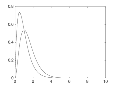
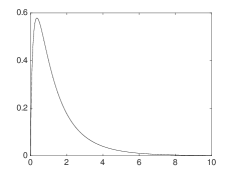
Figure 4.1. PDFs of the random variables $X$ and $Y$ (left) and PDF of the product random variable $Z=XY$ in Example 4.1.1 (right).

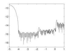
Figure 4.2. Error curve $\epsilon\left(x\right)$ (see (4.2)) in Example 4.1.1. Algorithm 2 was applied three times to obtain this result (see Remark 3.1).

4.1.2. Product of Nakagami random variables

The distributions of the product of Nakagami random variables have applications in wireless communication systems [29]. The PDF of a Nakagami distributed random variable is given by

(4.3) $$f^{\mathcal{N}}\left(x;m,\Omega\right)=\frac{2m^{m}}{\Gamma\left(m\right)\Omega^{m}}x^{2m-1}e^{-\frac{m}{\Omega}x^{2}},$$

where $m\geq 1/2$ and $\Omega>0$ are called the shape and spread parameters; as is well known, the Nakagami distribution is related to the Gamma and Chi distributions. In this example, we compute the PDFs of the product of two, four and eight Nakagami distributed random variables. Given the random variable $X\sim f^{\mathcal{N}}\left(x,1,1\right)=2xe^{-x^{2}}$ (see Figure 4.5), we first employ either Algorithm 1 or 2 on the Gaussian part of $f^{\mathcal{N}}$, $g\left(x\right)=2e^{-x^{2}}$, to obtain its approximation, $\tilde{g}\left(x\right)$, in the form (2.2) with $\alpha=1$. To obtain $\tilde{g}$ it is sufficient to sample $g$ on the interval $x\in\left[0,6\right]$ and use Algorithm 2 to solve (3.1) with $R=6$ and $N=500$, where we set $\epsilon=10^{-11}$. In Figure 4.3 we display the error,

(4.4) $$\epsilon\left(x\right)=\log_{10}\left(\left|g\left(10^{x}\right)-\tilde{g}(10^{x})\right|\right),\,\,\,-12\leq x\leq 1,$$

of the approximation via $\tilde{g}(x)$. Figure 4.4 shows the location of the complex nodes $\xi_{m}$ in the resulting representation of $\tilde{g}(x)$.

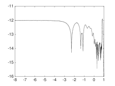
Figure 4.3. Error curve $\epsilon\left(x\right)$ (see (4.4)) in Example 4.1.2.

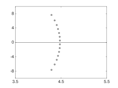
Figure 4.4. Complex nodes $\xi_{m}$ in the representation of $\tilde{g}(x)$ in Example 4.1.2. Horizontal and vertical axes correspond to $\mathcal{R}e\left(\xi_{m}\right)$ and $\mathcal{I}m\left(\xi_{m}\right)$, respectively.

After obtaining an accurate approximation $f_{X}$ of $f^{\mathcal{N}}$, using $\tilde{g}$ in the form (2.2), we compute the PDF $p_{Y}$ of the random variable $Y=X^{2}$ using (2.7) and display it in Figure 4.5. The exact product PDF is available analytically as $p\left(x\right)=4xK_{0}\left(2x\right)$, where $K_{0}$ is modified Bessel function of the second kind. The error,

(4.5) $$\epsilon\left(x\right)=\log_{10}\left(\left|p_{Y}\left(10^{x}\right)-p(10^{x})\right|\right),\,\,\,-8\leq x\leq 1,$$

is displayed in Figure 4.6. Figure 4.7 shows the location of the complex nodes $\xi_{m}$ in the representation of $p_{Y}$.

Using the computed PDF $p_{Y}$, we compute the PDF $p_{Z}$ of the product of four Nakagami distributed random variables, $Z=Y^{2}=X^{4}$ (see Figure 4.8). Likewise, we compute the PDF $p_{W}$ of the product of eight Nakagami random variables and display the result in Figure 4.9.

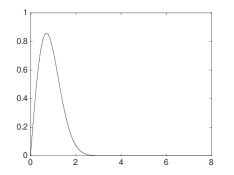
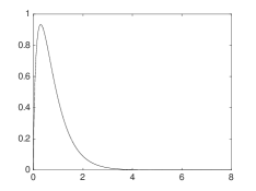
Figure 4.5. PDF of the random variable $X$ (left) and PDF of the product random variable $Y=X^{2}$ in Example 4.1.2 (right).

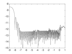
Figure 4.6. Error curve $\epsilon\left(x\right)$ (see (4.5)) in Example 4.1.2. Algorithm 2 was applied four times to obtain this result (see Remark 3.1).

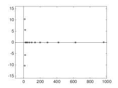
Figure 4.7. Complex nodes $\xi_{m}$ in the representation of the PDF $p_{Y}$ in Example 4.1.2. Horizontal and vertical axes correspond to $\mathcal{R}e\left(\xi_{m}\right)$ and $\mathcal{I}m\left(\xi_{m}\right)$, respectively.

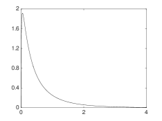
Figure 4.8. PDF of the random variable $Z=X^{4}$ in Example 4.1.2.

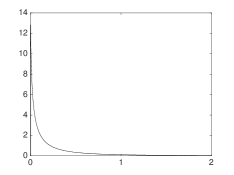
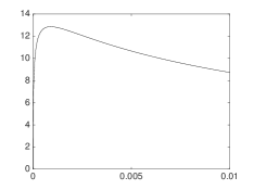
Figure 4.9. PDF of the random variable $W=X^{8}$ on the interval $x\in\left[0,2\right]$ (left) and on the interval $x\in\left[0,0.1\right]$ in Example 4.1.2 (right).

4.1.3. Product of Lomax and Gamma random variables

As another example, we compute the PDF of the product of a Gamma distributed random variable with PDF given by (4.1) and a Lomax distributed random variable with PDF given by

$$f^{\ell}\left(x;\alpha,\lambda\right)=\frac{\alpha}{\lambda}\left(1+\frac{x}{\lambda}\right)^{-\left(\alpha+1\right)},$$

where $\alpha>0$ and $\lambda>0$ are called the shape and scale parameters. In this example we use the Gamma distributed random variable $X\sim f^{\gamma}\left(x;3,2\right)$ and the Lomax distributed random variable $Y\sim f^{\ell}\left(y;5,2\right)$, and compute the PDF $p_{Z}$ of the product $Z=XY$. We illustrate the PDFs of the random variables $X$, $Y$, and $Z$ in Figure 4.10.

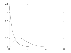
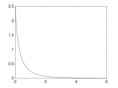
Figure 4.10. PDFs of the random variables $X$ and $Y$ (left) and the PDF of the product random variable $Z=XY$ in Example 4.1.3 (right).

4.1.4. Product of Weibull and Nakagami random variables

Next we consider the Weibull distributed random variable with PDF given by

$$f^{w}\left(x;\lambda,k\right)=\frac{k}{\lambda}\left(\frac{x}{\lambda}\right)^{k-1}e^{-\left(\frac{x}{\lambda}\right)^{k}},\,\,\,x\geq 0,$$

where $k>0$ and $\lambda>0$ are called the shape and scale parameters. We use a Weibull distributed random variable $X\sim f^{w}\left(x;1,1.5\right)$ and the random variable $Y$ obtained in Example 4.1.2 (the product of two Nakagami random variables), and compute the PDF $p_{Z}$ of the product $Z=XY$. We display the results in Figure 4.11.

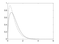
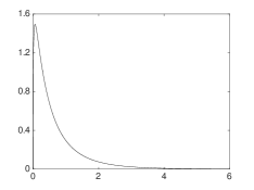
Figure 4.11. PDFs of the random variables $X$ and $Y$ (left) and the PDF of the product random variable $Z=XY$ in Example 4.1.4 (right).

4.1.5. Quotient of Nakagami and Gamma random variables

Finally, we compute the PDFs $p_{Z_{1}}$ and $p_{Z_{2}}$ of the quotients $Z_{1}=X/Y$ and $Z_{2}=Y/X$ of Nakagami and Gamma random variables $X$ and $Y.$ Given random variables $X\sim f^{\mathcal{N}}\left(x;1,1\right)$ as in Example 4.1.2 and $Y\sim f^{\gamma}\left(y,3,2\right)$ as in Example 4.1.1, we compute the PDFs of their ratios and display the results in Figure 4.12.

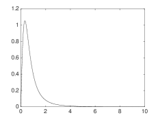
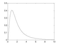
Figure 4.12. PDFs of the random variables $Z_{1}=X/Y$ (left) and $Z_{2}=Y/X$ (right) in Example 4.1.5.

4.1.6. Heavy-tailed distribution

Our approach remains valid for heavy-tailed distributions. As an example, let us consider a random variable $X$ with the standard Cauchy distribution,

(4.6) $$f_{exact}\left(x\right)=\frac{1}{\pi}\frac{1}{1+x^{2}}$$

and compute the distribution for $\left|X\right|^{2}$. In this case the integral defining the PDF of $\left|X\right|^{2}$ is evaluated explicitly,

(4.7) $$p_{exact}\left(t\right) = \int_{\mathbb{R}}\int_{\mathbb{R}}f\left(x\right)f\left(y\right)\delta\left(t-\left|x\right|\left|y\right|\right)dxdy$$

$$= \frac{4}{\pi^{2}}\int_{0}^{\infty}\int_{0}^{\infty}\frac{1}{1+x^{2}}\frac{1}{1+y^{2}}\delta\left(t-xy\right)dxdy$$

$$= \frac{4}{\pi^{2}}\int_{0}^{\infty}\frac{1}{1+x^{2}}\frac{1}{t^{2}+x^{2}}xdx$$

$$= \frac{4}{\pi^{2}}\frac{\log\left(t\right)}{t^{2}-1},$$

which allows us to estimate the error of our numerical approach. We start by approximating the Cauchy distribution (4.6) via exponentials in the form (2.2). Using the Laplace transform, we have

(4.8) $$f_{exact}\left(x\right)=\frac{1}{\pi}\int_{0}^{\infty}e^{-x\tau}\sin\left(\tau\right)d\tau=\frac{1}{\pi}\int_{-\infty}^{\infty}e^{-xe^{s}+s}\sin\left(e^{s}\right)ds.$$

Unfortunately, discretizing this integral directly via the trapezoidal rule requires too many terms to achieve an accurate approximation for small values of $x$. Therefore, we discretize (4.8) only to approximate the tail of (4.6). We obtain

(4.9) $$\left|f_{exact}\left(x\right)-f_{tail}\left(x\right)\right|\leq\epsilon,\,\,\,x\in\left[7.4748,\infty\right),$$

where

$$f_{tail}\left(x\right)=h_{0}\sum_{j=M}^{N}e^{-xe^{s_{j}}+s_{j}}\sin\left(e^{s_{j}}\right)$$

with $s_{j}=jh_{0}$, $h_{0}=0.25$, $M=-70$ and $N=5$, and achieve accuracy $\epsilon\approx 10^{-15}$. We then consider the difference $f_{head}\left(x\right)=f_{exact}\left(x\right)-f_{tail}\left(x\right)$ in the interval $\left[0,7.4748\right]$ and use Algorithms 1 or 2 to obtain an approximation for $f_{head}\left(x\right)$ with $15$ terms. Finally, we remove all terms of $f_{head}\left(x\right)+f_{tail}\left(x\right)$ with weights less than $0.33\cdot 10^{-12}$ leaving $73$ terms in the resulting approximation of $f_{exact}\left(x\right)$. In Figure 4.13 we display the exponents and the error of the resulting approximation,

(4.10) $$\mbox{err}_{f}\left(s\right)=\log_{10}\left(\left|f_{exact}\left(10^{s}\right)-f_{tail}\left(10^{s}\right)-f_{head}\left(10^{s}\right)\right|+10^{-20}\right),\,\,\,s\in\left[-15,6\right].$$

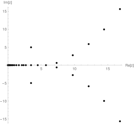
Figure 4.13. The $73$ exponents of the approximation of the PDF (4.6) (left) and log-log plot of the resulting approximation error (4.10) (right).

To compute an approximation for the distribution of $\left|X\right|^{2}$, we use $p\left(t\right)$ in Lemma 2.2 where $\alpha=\beta=1$ and, thus,

(4.11) $$p\left(t\right)=v\left(t\right)=2\sum_{m=1}^{M}\sum_{n=1}^{N}a_{m}b_{n}K_{0}\left(2\sqrt{t\xi_{m}\eta_{n}}\right).$$

In order to find an exponential approximation for $p\left(t\right)$, we first use $40,000$ equally spaced points with step size $h=2$ to discretize (4.11) and use Algorithms 1 or 2 to approximate the “tail” of $p$. The resulting approximation with $30$ terms is valid in the interval $\left[9.18,\infty\right)$. We then consider the difference $p_{head}^{1}\left(t\right)=p\left(t\right)-\widetilde{p}_{tail}\left(t\right)$ in the interval $\left[10^{-4},9.18\right]$, discretize $p_{head}^{1}\left(t\right)$ in this interval using $100,000$ equally spaced points, and use one of the mentioned algorithms to obtain an approximation for $p_{head}^{1}\left(t\right)$ with $40$ terms. We then consider $p_{head}^{2}\left(t\right)=p\left(t\right)-\widetilde{p}_{tail}\left(t\right)-p_{head}^{1}\left(t\right)$ in the interval $\left[10^{-7},0.5814\cdot 10^{-3}\right]$, discretize $p_{head}^{2}\left(t\right)$ in this interval using $50,000$ equally spaced points, and again use Algorithms 1 or 2 to obtain an approximation for $p_{head}^{2}\left(t\right)$ with $25$ terms. In Figure 4.14 we display the error of the final approximation with $95$ terms,

(4.12) $$\mbox{err}_{p}\left(y\right)=\log_{10}\left(\left|p_{exact}\left(10^{y}\right)-\widetilde{p}_{tail}\left(10^{y}\right)-p_{head}^{1}\left(10^{y}\right)-p_{head}^{2}\left(10^{y}\right)\right|+10^{-20}\right),$$

where $y\in\left[-7,8\right]$. We note that in this example we were not seeking an optimal representation of the form (2.2) of the distribution for $\left|X\right|^{2}$.

Figure 4.14. Log-log plot of the error (4.12) of approximating the PDF (4.7) with $95$ terms.

5. Computing expectations of functions of random variables

An important use of representing the PDF $p_{Z}$ of a non-negative random variable in the proposed functional form is to compute, for a function $u$, the expectation of the variable $u\left(Z\right)$,

(5.1) $$\mbox{E}\left[u\left(Z\right)\right]=\int_{0}^{\infty}u\left(x\right)p_{Z}\left(x\right)dx.$$

If the function $u$ is given analytically, i.e. we can evaluate it at any point, the fact that we have a functional representation of $p_{Z}$ allows us to use an appropriate quadrature to evaluate this integral to any desired accuracy. Moreover, if the function $u$ admits a representation via exponentials (which can be computed via Algorithms 1 or 2), the expectation (5.1) can be evaluated explicitly. If only samples of the function $u$ are provided, then we can treat $p_{Z}$ as a weight and construct a quadrature with nodes at locations where the values of $u$ are available. If the function $u$ is a monomial, i.e. when computing the moments of random variable $Z$, we can use the explicit integral

$$\int_{0}^{\infty}x^{\alpha-1}e^{-\eta x}dx=\eta^{-\alpha}\Gamma\left(\alpha\right),\ \ \mathcal{R}e\left(\eta\right)>0,\ \ \alpha>0.$$

For example, given the PDF of a random variable $Z$ in the form (2.2), we compute its first moment $m_{1}$ as

$$m_{1}=\Gamma\left(\alpha+1\right)\sum_{l=1}^{M}a_{l}\xi_{l}^{-\left(\alpha+1\right)},$$

and its second moment $m_{2}$ as

$$m_{2}=\Gamma\left(\alpha+2\right)\sum_{l=1}^{M}a_{l}\xi_{l}^{-\left(\alpha+2\right)}-m_{1}.$$

We note that while our algorithms do not guarantee that the moments are preserved exactly, the accuracy of the resulting moments is controlled by the overall accuracy of the approximation. In particular, we can always enforce $\int_{0}^{\infty}p_{Z}\left(x\right)dx=1$ by imposing an additional linear constrain on the coefficients $a_{l}$ of the exponential approximation.

6. Conclusions and further work

For any user-selected accuracy, we have developed an approximate representation of non-negative random variables (2.2) that allow us to compute the PDFs of their sums, products and quotients in the same functional form. The monomial factor in the functional form in (2.2) is chosen to accommodate a possible rapid change of the PDFs of non-negative random variables near zero.

We demonstrated accuracy and efficiency of the resulting numerical calculus of PDFs on several numerical examples. In order to account for the boundary at zero, we use a different representation of the PDFs of non-negative random variables than our previous construction for random variables defined on the whole real line [9]. Clearly, Gaussian mixtures used in [9] do not have support restricted to the positive real axis and, thus, could not yield an efficient representation.

While there are clear advantages to our new approach for computing PDFs in comparison with Monte Carlo-type methods, we do not compare the two in this paper. We plan to address such comparison elsewhere in the context of practical applications.

References

- [1] M. Abramowitz and I. A. Stegun. Handbook of mathematical functions. Dover Publications, 9 edition, 1970.
- [2] V. M. Adamjan, D. Z. Arov, and M. G. Kreĭn. Infinite Hankel matrices and generalized Carathéodory-Fejér and I. Schur problems. Funkcional. Anal. i Priložen., 2(4):1–17, 1968.
- [3] V. M. Adamjan, D. Z. Arov, and M. G. Kreĭn. Infinite Hankel matrices and generalized problems of Carathéodory-Fejér and F. Riesz. Funkcional. Anal. i Priložen., 2(1):1–19, 1968.
- [4] V. M. Adamjan, D. Z. Arov, and M. G. Kreĭn. Analytic properties of the Schmidt pairs of a Hankel operator and the generalized Schur-Takagi problem. Math. USSR Sbornik, 15(1):34–75, 1971.
- [5] G. E. Andrews, R. Askey, and R. Roy. Special functions, volume 71 of Encyclopedia of Mathematics and its Applications. Cambridge University Press, Cambridge, 1999.
- [6] G. Beylkin and L. Monzón. On approximation of functions by exponential sums. Appl. Comput. Harmon. Anal., 19(1):17–48, 2005.
- [7] G. Beylkin and L. Monzón. Nonlinear inversion of a band-limited Fourier transform. Appl. Comput. Harmon. Anal., 27(3):351–366, 2009.
- [8] G. Beylkin and L. Monzón. Approximation of functions by exponential sums revisited. Appl. Comput. Harmon. Anal., 28(2):131–149, 2010.
- [9] G. Beylkin, L. Monzón, and I. Satkauskas. On computing distributions of products of random variables via Gaussian multiresolution analysis. Appl. Comput. Harmon. Anal., 2017. doi: 10.1016/j.acha.2017.08.008, see also arXiv:1611.08580.
- [10] Y. Chen, G. K. Karagiannidis, H. Lu, and N. Cao. Novel approximations to the statistics of products of independent random variables and their applications in wireless communications. IEEE Transactions on Vehicular Technology, 61(2):443–454, 2012.
- [11] H. Cheng, Z. Gimbutas, P.-G. Martinsson, and V. Rokhlin. On the compression of low-rank matrices. SIAM Journal of Scientific Computing, 205(1):1389–1404, 2005.
- [12] NIST Digital Library of Mathematical Functions. http://dlmf.nist.gov/, Release 1.0.13 of 2016-09-16. F. W. J. Olver, A. B. Olde Daalhuis, D. W. Lozier, B. I. Schneider, R. F. Boisvert, C. W. Clark, B. R. Miller and B. V. Saunders, eds.
- [13] B. Epstein. Some applications of the Mellin transform in statistics. The Annals of Mathematical Statistics, pages 370–379, 1948.
- [14] I. S. Gradshteyn and I. M. Ryzhik. Table of integrals, series, and products. Elsevier/Academic Press, Amsterdam, eighth edition, 2015. Translated from the Russian, Translation edited and with a preface by Daniel Zwillinger and Victor Moll, Revised from the seventh edition [MR2360010].
- [15] N. Halko, P.-G. Martinsson, and J. A. Tropp. Finding structure with randomness: probabilistic algorithms for constructing approximate matrix decompositions. SIAM Review, 53(2):217–288, 2011.
- [16] T. S. Haut and G. Beylkin. Fast and accurate con-eigenvalue algorithm for optimal rational approximations. SIAM J. Matrix Anal. Appl., 33(4):1101–1125, 2012. doi: 10.1137/110821901.
- [17] R. A. Horn and C. R. Johnson. Matrix analysis. Cambridge University Press, Cambridge, 1990.
- [18] Y. Hua and T.K. Sarkar. Matrix pencil method and its performance. In Proceedings of the International Conference on Acoustics, Speech, and Signal Processing, volume 4, pages 2476–2479, 1988.
- [19] Y. Hua and T.K. Sarkar. Matrix pencil method for estimating parameters of exponentially damped/undamped sinusoids in noise. IEEE Transactions on Acoustics, Speech, and Signal Processing, 38(5):814–824, 1990.
- [20] Y. Hua and T.K. Sarkar. On SVD for estimating generalized eigenvalues of singular matrix pencil in noise. IEEE Transactions on Signal Processing, 39(4):892–900, 1991.
- [21] S.Y. Kung, K.S. Arun, and D.V. Bhaskar Rao. State-space and singular-value decomposition-based approximation methods for the harmonic retrieval problem. Journal of the Optical Society of America, 73(12):1799–1811, 1983.
- [22] E. Liberty, F. Woolfe, P-G. Martinsson, V. Rokhlin, and M. Tygert. Randomized algorithms for the low-rank approximation of matrices. Proc. Natl. Acad. Sci. USA, 104(51):20167–20172, 2007.
- [23] Z.A. Lomnicki. On the distribution of products of random variables. Journal of the Royal Statistical Society. Series B (Methodological), pages 513–524, 1967.
- [24] S. Nadarajah and S. Kotz. On the product and ratio of Gamma and Weibull random variables. Econometric Theory, 22(02):338–344, 2006.
- [25] M. Reynolds, G. Beylkin, and L. Monzón. Rational approximations for tomographic reconstructions. Inverse Problems, 29(6):065020, 23pp, 2013.
- [26] M. Shakil and B.M. Kibria. On the product of Maxwell and Rice random variables. Journal of Modern Applied Statistical Methods, 6(1):212–218, 2007.
- [27] M.D. Springer. Algebra of Random Variables. John Wiley & Sons, 1979.
- [28] M.D. Springer and W.E. Thompson. The distribution of products of independent random variables. SIAM Journal on Applied Mathematics, 14(3):511–526, 1966.
- [29] Z. Zheng, L. Wei, J. Hamalainen, and O. Tirkkonen. Approximation to distribution of product of random variables using orthogonal polynomials for lognormal density. IEEE Communications Letters, 16(12):2028–2031, 2012.