Stochastic Gradient Descent for Relational Logistic Regression via
Partial Network Crawls
Abstract
Research in statistical relational learning has produced a number of methods for learning relational models from large-scale network data. While these methods have been successfully applied in various domains, they have been developed under the unrealistic assumption of full data access. In practice, however, the data are often collected by crawling the network, due to proprietary access, limited resources, and privacy concerns. Recently, we showed that the parameter estimates for relational Bayes classifiers computed from network samples collected by existing network crawlers can be quite inaccurate, and developed a crawl-aware estimation method for such models (Yang, Ribeiro, and Neville, 2017). In this work, we extend the methodology to learning relational logistic regression models via stochastic gradient descent from partial network crawls, and show that the proposed method yields accurate parameter estimates and confidence intervals.
1 Introduction
There has been a great deal of interest in learning statistical models that can represent and reason about relational dependencies (see e.g., Getoor and Taskar, 2007). For example, political views are often correlated among friends in social networks. While much work has been done in the relational learning community to develop models and algorithms for estimation and inference in networks, a primary assumption underlying these works is that a full network is available for learning. With access to the full network, one could perform stochastic gradient descent (SGD) in the usual manner, and the learned parameters will asymptotically converge to the desired parameter estimates (Robbins and Monro, 1951; Bottou and Le Cun, 2005; Bach, 2014).
However, the network datasets used to study relational models are typically samples of a larger network. In particular, it is often the case that researchers do not have random access to the full network structure and that sampling is only possible via repeated crawling from a node to its neighbors—a procedure that tends to result in biased samples (Kurant, Markopoulou, and Thiran, 2011; Ribeiro and Towsley, 2012). As a result, naively performing SGD using these partial crawls may also suffer from unknown biases. Part of this work shows that such crawled data could indeed lead to biased parameter estimates in real-world scenarios.
Recently, we showed that estimating the parameters in a relational Bayes classifier (RBC) (Neville, Jensen, and Gallagher, 2003; Macskassy and Provost, 2007) using data from widely used network sampling methods—such as snowball sampling, forest-fire (Leskovec and Faloutsos, 2006), random walks, and Metropolis-Hastings random walk (Gjoka et al., 2010)—could lead to biased parameter estimates (Yang, Ribeiro, and Neville, 2017). We then corrected for such estimation bias in the RBC by exploiting a general crawling method introduced by Avrachenkov, Ribeiro, and Sreedharan (2016) that produces unbiased estimates with statistical guarantees.
In this work, we extend the methodology to develop a crawl-based SGD procedure for relational logistic regression (RLR). The proposed method is guaranteed to obtain unbiased estimates of the log-likelihood function and its gradients over the full network (with finite variance), which allows SGD to converge to the correct parameter values for sufficiently small learning rates (Robbins and Monro, 1951). Furthermore, we show how to construct confidence intervals of the estimated parameters, which enables practitioners to assess the statistical significance of features in the model.
Summary of Contributions
-
•
We derive a crawl-based SGD method for learning the RLR model from partial network crawls, and prove that the proposed method yields unbiased estimates of the log-likelihood function and its gradients over the full network.
-
•
We demonstrate how to construct confidence intervals of the estimated parameters by exploiting the independence properties of the network samples.
-
•
We conduct experiments on several large network datasets, and demonstrate that the proposed methodology achieves consistently lower error in parameter estimates and higher coverage probabilities of confidence intervals.
2 Problem Definition
The goal of this work is to develop a stochastic estimation algorithm for the relational logistic regression (RLR) model in large social networks under an access-restricted scenario. In particular, we are interested in accurately estimating model parameters in order to effectively assess the importance of relational features involving the neighbors of a node.111In Yang, Ribeiro, and Neville (2017), we also referred to the parameters in a relational model as peer effects.
We assume that random access to the full network structure is not available, and that the network can only be accessed via crawling. Specifically, we assume (i) the availability of a seed node in the network, (ii) the ability to query for the attributes of a sampled node, and (iii) the ability to transition to neighbors of a sampled node.
Given such an access pattern, and assuming that the full network cannot be crawled, the task is to accurately estimate the model parameters by learning an RLR model over the sampled network. If we refer to the estimates that a learning algorithm would obtain from the full network as global estimates and those from the sampled network as sample estimates, then the ideal method should produce (i) unbiased sample estimates (w.r.t. the global estimates), and (ii) accurate assessments of the uncertainty associated with the sample estimates (e.g., confidence intervals).
3 Background and Related Work
Denote a graph by , where is the set of vertices and is the set of edges. For a node , denote its neighbors by and its degree by . Finally, let denote the indicator function.
Network Sampling Algorithms
We note that under a crawl-based scenario, any technique involving random node/edge selection will be infeasible.
Snowball sampling (BFS) traverses the network via a breadth-first search. Forest fire (FF) (Leskovec and Faloutsos, 2006) samples (“burns”) a random fraction of a node’s neighbors, and repeats this process recursively for each “burned” neighbor. Random walk sampling (RW) performs a random walk on the network by transitioning from the current node to a randomly selected neighbor at every step. Metropolis-Hastings random walk (MH) (Gjoka et al., 2010) sets the transition probability from node to as if and if , which yields a uniform stationary distribution over nodes.
Random walk tour sampling (TS) (Avrachenkov, Ribeiro, and Sreedharan, 2016) is a recently proposed method that exploits the regenerative properties of random walks. Given an initial seed node, the algorithm first performs a short random walk to collect a set of seed nodes , and then proceeds to sample a sequence of random walk tours. Specifically, the -th random walk tour starts from a sampled node and transitions through a sequence of nodes until it returns to a node . The algorithm repeats this process to sample such tours, denoted . Since the successive returns to a seed node in act as renewal epochs, the renewal reward theorem (Brémaud, 1999) guarantees that sample statistics computed from each tour will be independent.
Relational Learning Models
Relational learning models (see e.g., Getoor and Taskar, 2007) extend traditional supervised learning methods to the relational domain, in which training examples (such as nodes in a social network) are no longer i.i.d. (independent and identically distributed).
Relational logistic regression (RLR) (see e.g., Kazemi et al., 2014) predicts the target class of a node using aggregated features constructed from the class label and attributes of its neighbors. A typical aggregation function is proportion, which takes the proportion of neighbors that possess a particular class label or feature value. Let be a set of aggregated features for node that involve either the attributes of or the attributes/class label of its neighbors . Let be the class label of node . The RLR model employs the soft-max function to predict :
where are the weights for class that need to be estimated from the network.
Related Work
In our previous work (Yang, Ribeiro, and Neville, 2017), we showed that the class priors and conditional probability distributions (CPDs) in a relational Bayes classifier (RBC) can be unbiasedly estimated under the same crawl-based scenario that we consider here. In this work, we extend the methodology to the estimation of RLR models using a crawl-based SGD method. Note that RLR forms a more expressive model family which poses a more challenging estimation task—in fact, the CPDs in an RBC can be implicitly represented by features in an RLR model. Furthermore, statistical significance tests (e.g., and deviance tests) for the parameter estimates in an RLR model have been extensively studied (see e.g., Agresti, 2002) in the literature, which offer tools for feature selection and model comparison.
4 Proposed Methodology
Given an unobserved network , the tasks are (i) to estimate the parameters in a relational model by crawling the network from an initial set of seed nodes , and (ii) to assess the uncertainty associated with the estimates . To this end, we outlined the following procedure for crawl-based estimation of relational models in large-scale networks (Yang, Ribeiro, and Neville, 2017):
- missingfnum@@desciitemCrawling
-
Crawl the network using a sampling method.
- missingfnum@@desciitemEstimation
-
Estimate parameters from the crawled network.
- missingfnum@@desciitemCalibration
-
Compute confidence intervals for the estimates.
For the crawling phase, we shall employ the random walk tour sampling algorithm (see Section 3). Next, we discuss the details of our proposed stochastic estimation and calibration methodology for relational logistic regression (RLR).
Relational Model Estimation
Recall that RLR utilizes a multinomial logistic regression model to define conditional probability of the label of node given its observed attributes and the attributes/class label of its neighbors . Let be a set of aggregated features for node that is computed from its neighbors . In practice, to reduce the node-querying cost, we can estimate the aggregated features stochastically by taking a uniform sample of the neighbors . The log-likelihood for the RLR model is given by
| (1) |
where are the weights for class .
In general, we do not have any guarantees on the quality of the parameter estimates obtained from a crawled network. However, if the sample were collected using the tour sampling algorithm, we propose applying Theorem 1 to accurately estimate the parameters in an RLR model.
Theorem 1 (RLR crawl-based SGD)
Given the sampled random walk tours , the following estimates for the log-likelihood of Eq. (1) and its gradients are unbiased:
| (2) | ||||
| (3) |
where denotes the total number of outgoing edges from the seed nodes, and
Proof
We defer the proof to the Appendix.
We can learn the weights of an RLR model by minimizing the negative
log-likelihood via stochastic gradient descent using the
estimates of Eq. (3).
While Theorem 1 shows that the log-likelihood over the full network
and its gradients can be unbiasedly estimated, we note that the current result
does not directly imply bounds on the approximation error of the resulting parameter estimates.
Empirically, our experiments suggest that the parameter estimates are quite accurate.
Calibration of Estimated Parameters
To construct confidence intervals for the estimated parameters, we propose to utilize bootstrap resampling (Efron, 1979). In fact, this step can be performed as sampling progresses—by monitoring the confidence intervals, the practitioner can determine adaptively if more samples need to be collected.
For tours sampling, since the estimates computed from each tour are independent, we can perform bootstrapping by treating the tours individually, sample with replacement, compute an estimate over the bootstrap sample, and repeat this process. We can then compute empirical confidence intervals over the bootstrap estimates. Algorithm 1 describes the bootstrapping algorithm we use to compute confidence intervals for the parameters in a general relational model. For convenience, denote the nodes sampled in the -th tour by .
Among all the crawling methods under examination, tours sampling is the only approach capable of producing theoretically justified confidence intervals via resampling. This is due to the fact that BFS, FF, RW, and MH do not provide a list of node/edge samples that yield i.i.d. estimates of the model parameters.
5 Experimental Evaluation
Dataset Description
We perform experiments on five different attributed network datasets. As a preprocessing step, we take the giant component of all networks. Table 1 shows the summary statistics for each network after processing.
| Dataset | Attributes | Class Prior Distribution | ||
|---|---|---|---|---|
| 14,643 | 336,034 | PoliticalView | Conservative: 28.40%, Otherwise: 71.60% | |
| Friendster-Large | 3,146,011 | 47,660,702 | Age | [16, 26): 35.02%, [26, 28): 16.27%, [28, 32): 22.56%, [32: 100): 26.15% |
| Gender | Female: 46.99%, Male: 53.01% | |||
| Status | Single: 67.21%, In a Relationship: 19.06%, Married: 12.60%, Domestic Partner: 1.13% | |||
| Friendster-Small | 1,120,930 | 19,342,990 | Age | [16, 26): 44.53%, [26, 28): 14.96%, [28, 32): 21.28%, [32, 100): 19.23% |
| Gender | Female: 45.39%, Male: 54.61% | |||
| Status | Single: 62.01%, In a Relationship: 20.29%, Married: 16.50%, Domestic Partner: 1.21% | |||
| Zodiac | Capricorn: 7.74%, Virgo: 8.27%, Libra: 8.60%, Gemini: 8.11%, | |||
| Scorpio: 8.31%, Leo: 8.88%, Taurus: 8.79%, Sagittarius: 8.58%, | ||||
| Cancer: 8.15%, Aquarius: 8.97%, Pisces: 7.83%, Aries: 7.77% | ||||
| Communications | 855,172 | 5,269,278 | Comm. | Yes: 6.09%, No: 93.91% |
| Computers | 855,172 | 5,269,278 | Computers | Yes: 17.34%, No: 82.66% |
Facebook is a snapshot of the Purdue University Facebook network consisting of users who have listed their political views (whether or not they declare to be conservative).
Friendster-Large (Fri.-L.) and Friendster-Small (Fri.-S.) are processed from the entire Friendster social network crawl (Mouli et al., 2017). For Fri.-L., we take the subgraph containing all users with age, gender, and marital status listed in their profiles. For Fri.-S., we also include zodiac. We discretized the age attribute into four interval classes.
The observations we make are not restricted to social networks. We also experiment on two citation networks, Communications (Comm.) and Computers, both constructed from the NBER patent citations dataset (Hall, Jaffe, and Trajtenberg, 2001).222While the edges in the citation networks are directed, we treat them as undirected edges in the experiments for simplicity. The label of each patent indicates whether it was filed in a category related to comm. (computers).
Experiment Setup
In each run of the simulation, we randomly select 50% nodes in the network to have observed labels, and the task is to infer the labels of the remaining nodes. Next, a labeled node is randomly selected as the seed node to initiate crawling for all the sampling methods.333In practice, one could always avoid querying unlabeled nodes; thus, we set all methods to crawl directly on the labeled subgraph. In practice, querying a node will be associated with a certain cost, and we strictly control for the number of unique node-queries. For each method, we keep track of the parameter estimates and bootstrap confidence intervals as crawling progresses. We perform 10 runs of the simulation, and report the average performance and standard errors for all methods.
Evaluation Criteria
We measure the performance of the various network crawling methods in terms of:
-
•
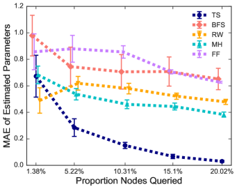
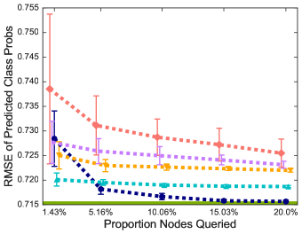
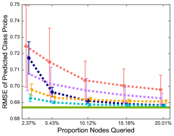
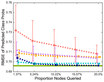
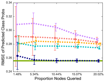
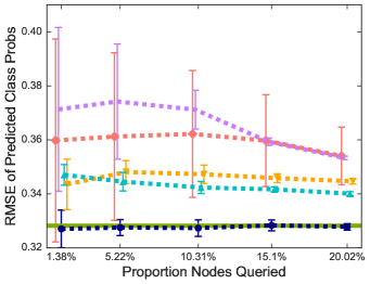
The quality of the RLR parameter estimates learned from a network sample crawled using that method. Specifically, we measure (i) the mean-absolute-error (MAE) between the sample estimate computed from the crawled sample and the global estimate computed from the entire graph, and (ii) the root-mean-square-error (RMSE) of the predicted class probabilities for the unlabeled nodes444 When predicting the class label for an unlabeled node, in addition to the attributes and class label of its neighbors, the attributes (but not the class label) of the unlabeled node are also available. using an RLR model equipped with the sample estimates.
-
•
The quality of the confidence intervals obtained from the crawled sample, as measured by the coverage probability.
Evaluation of Estimation Performance
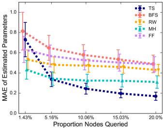
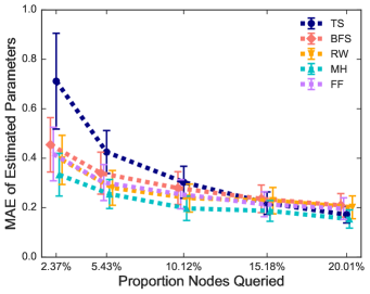
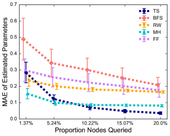
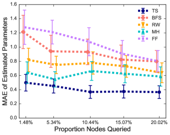
Figure 1 shows the quality of the estimated parameters vs. the proportion of queried nodes as crawling progresses.555For the Friendster results, the parenthesized attribute denotes the class label used for the prediction task, while all other attributes are used as features. The solid line in the RMSE plots correspond to the prediction error obtained using the global estimates. The plots are jittered horizontally to prevent the error bars from overlapping. We observe that across all datasets, tour sampling (TS) consistently achieves smaller MAE in the estimated model parameters as well as lower RMSE in the predicted class probabilities. Also note that MH and RW usually outperfom FF and BFS.
For numerical stability reasons, we utilized either or regularization in our experiments. Since our interest is in accurately estimating model parameters, we set the regularization parameter to be very small () in both cases. Not surprisingly, regularization results in sparser parameter estimates. Also note that the unbiased estimators we proposed for TS automatically scales up the estimate of the log-likelihood and its gradients to match that of the full-network, whereas those obtained using conventional sampling methods would depend on the size of the crawled sample.
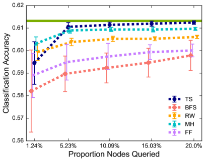
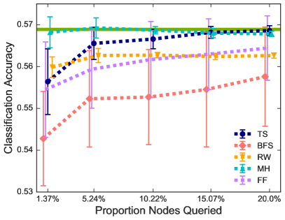
Comparing the learning curves for the parameter estimates MAE with those of the RMSE of predicted class probabilities as well as the classification accuracy, we notice that the required sample size to achieve reasonable prediction performance can be much smaller than the sample size required to accurately estimate model parameters. Figure 2 also shows that more accurate parameter estimates do not necessarily translate to improved classification accuracy, as in some cases biased parameter estimates may lead to better generalization performance.
Evaluation of Calibration Performance
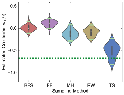
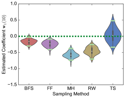
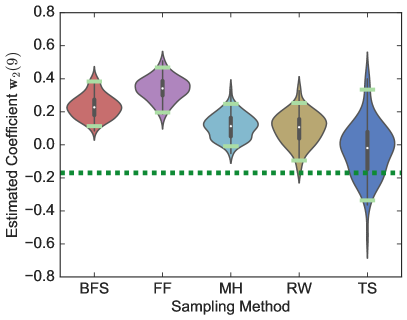
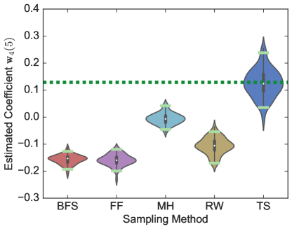
Figure 3 shows the estimated bootstrap sampling distributions for several model parameters.666For BFS, FF, RW, and MH, we perform bootstrapping directly on the sampled nodes by treating each node as an i.i.d. instance. We observe that TS is the only method consistently capturing the global parameter values.
To assess the calibration performance of each method, we compute 95% confidence intervals for the RLR parameters across 200 repeated trials, and calculate their empirical coverage probability (i.e., the proportion of trials in which the estimated confidence interval contains the global estimate) as well as average interval width. Table 2 shows the results when 15% of each network have been crawled. We observe that the coverage probability for TS is higher than every other method across all datasets.777Notice that in some cases, even TS does not achieve the nominal 95% coverage probability, possibly due to small errors in the parameter estimates when the crawling proportion is relatively low. Furthermore, regularization introduces an additional source of bias. In particular, notice that the coverage probabilities of RLR- are significantly lower than that of RLR- across all methods, which is due to the shrinkage effect of the penalty that results in parameter estimates with small values to be shrunk to exactly zero.
| (Coverage Probability, Average Interval Width) | ||||||
|---|---|---|---|---|---|---|
| Model | Dataset | BFS | FF | MH | RW | TS |
| RLR- | Fri.-L. (Age) | (0.0842, 0.1849) | (0.0801, 0.1940) | (0.1887, 0.2439) | (0.1615, 0.2674) | (0.7142, 0.5313) |
| RLR- | Fri.-L. (Gender) | (0.0714, 0.0757) | (0.0741, 0.0986) | (0.1278, 0.0979) | (0.1019, 0.1177) | (0.5239, 0.2167) |
| RLR- | Fri.-L. (Status) | (0.1946, 0.2636) | (0.1470, 0.2500) | (0.4548, 0.3876) | (0.3179, 0.3577) | (0.7479, 0.7591) |
| RLR- | Fri.-S. (Gender) | (0.4825, 0.2523) | (0.4810, 0.2886) | (0.7307, 0.3941) | (0.6346, 0.4384) | (0.7443, 0.8247) |
| RLR- | Comm. | (0.0000, 0.1475) | (0.0000, 0.1205) | (0.0000, 0.1817) | (0.0000, 0.1888) | (0.6240, 0.4346) |
| RLR- | Computers | (0.0000, 0.1008) | (0.0000, 0.1034) | (0.0000, 0.1268) | (0.0000, 0.1206) | (0.2500, 0.3595) |
| RLR- | Fri.-L. (Age) | (0.1393, 0.1739) | (0.1912, 0.1897) | (0.3687, 0.2457) | (0.3392, 0.2590) | (0.8321, 0.5160) |
| RLR- | Fri.-L. (Gender) | (0.1429, 0.0824) | (0.1429, 0.0863) | (0.3641, 0.0977) | (0.3552, 0.1045) | (0.9996, 0.2282) |
| RLR- | Fri.-L. (Status) | (0.3090, 0.2576) | (0.3055, 0.2765) | (0.5339, 0.3391) | (0.4078, 0.3331) | (0.8707, 0.7261) |
| RLR- | Fri.-S. (Gender) | (0.5508, 0.2606) | (0.6001, 0.2858) | (0.6722, 0.3909) | (0.7502, 0.4220) | (0.9568, 0.6578) |
| RLR- | Comm. | (0.0000, 0.1464) | (0.0000, 0.1556) | (0.0000, 0.2026) | (0.0000, 0.2100) | (1.0000, 0.5279) |
| RLR- | Computers | (0.0000, 0.1099) | (0.0000, 0.1296) | (0.0000, 0.1522) | (0.0000, 0.1462) | (1.0000, 0.3480) |
6 Conclusion and Future Work
In this work, we developed a stochastic gradient descent method for learning relational logistic regression models from large-scale networks via partial crawling. We proved that the proposed method yields unbiased estimates of the log-likelihood and its gradients over the full graph, and demonstrated how to construct confidence intervals of the model parameters. Our experiments showed that the proposed method produces more accurate parameter estimates and confidence intervals compared to naively learning models from data collected by existing crawlers.
Estimation of Templated Relational Models
One line of future work would be to extend our stochastic estimation method to the family of templated relational models, such as relational Markov networks (RMNs) (Taskar, Abbeel, and Koller, 2002), Markov logic networks (MLNs) (Domingos and Richardson, 2004), and relational dependency networks (RDNs) (Neville and Jensen, 2007) under the same crawl-based scenario examined in this work.
Notice that RLR can be viewed as a direct analog of MLNs where the weighted logic formulas are used to define conditional instead of joint probabilities. More generally, when the cliques in RMNs and MLNs are defined over connected subgraphs up to size three, we expect that the full log-likelihood can be unbiasedly estimated by extending our proposed methodology. However, learning RMNs and MLNs that contain higher-order clique structures would be more challenging.
For RDNs, the estimation procedure depends on the specific local conditional model one employs. Our previous work (Yang, Ribeiro, and Neville, 2017) can be used to learn RDNs when the RBC is used to model the local conditional probability distributions (CPDs), and the current work has addressed the case when RLR is used as the local model component. Another possible choice for the local model consist of relational probability trees (RPTs) (Neville et al., 2003). Similar to RLR, RPTs also utilize aggregation functions to construct node-centric features. While these aggregated features can be stochastically estimated in the same way as in RLR, learning the full tree structure becomes difficult due to the greedy partitioning procedure involved.
Impact of Sampling on Collective Inference
Finally, we note that in this work we utilize non-collective inference on the full graph—that is, when predicting an unlabeled node, we do not utilize the predictions made for its unlabeled neighbors, and instead treat their class labels as missing. Although collective inference has been shown to improve classification accuracy, it also introduces inference error (Xiang and Neville, 2011). In this work, we have mainly focused on examining the impact of crawling on learning, but future work should investigate the more complex interplay between sampling, learning, and inference.
Acknowledgements
This research is supported by NSF under contract numbers IIS-1149789, IIS-1546488, IIS-1618690, and by the Army Research Laboratory under Cooperative Agreement Number W911NF-09-2-0053.
Appendix A Proofs of Theorems
Proof of Theorem 1. It will be convenient to define the function
| (4) |
Recall that our goal is to estimate
| (5) |
where can be computed explicitly. Notice that888Recall that for undirected graphs, the edge-set contains both copies of each edge—i.e., if and only if .
| (6) |
Given the random walk tours , we estimate using , where
| (7) |
Here, denotes the total number of outgoing edges from the seed nodes, and the last equality follows from Eq. (4). Plugging the estimate into Eq. (5), we arrive at the full estimate of :
| (8) |
Moreover, the gradients of can be estimated by
| (9) |
To show that the estimates of Eqs. (8) and (8) are unbiased, it suffices to show that for all , is an unbiased estimate of , since the sample average will also be unbiased, and the gradient is a linear operator. More formally, we prove that for any , we have
| (10) |
Notice that the random walk tour sampling algorithm (cf. Section 3) is equivalent to a conventional random walk conducted on a virtual multi-graph formed by treating all the seed nodes in as a single “super-node” while retaining all outgoing edges. Thus, the degree of the super-node is . The sampling process, viewed as a random walk on , constitutes a renewal process in which a renewal occurs when the walk returns to the super-node (thereby completing a tour). For the -th tour , define its reward as
where and are two adjacent vertices in . By the Markov property, both the tour lengths and the rewards are i.i.d. sequences. Let
be the number of renewals (visits to the super-node) up to sampling the -th node in the random walk. Then the renewal reward theorem (Brémaud, 1999, Chapter 3, Theorem 4.2) implies that
| (11) |
Let be the edge-set of . The stationary probability of a random walk on are given by , and the transition probability from to is given by . Therefore,
| (12) |
and the mean recurrence time is . Joining Eq. (11) and Eq. (12), and multiplying by on both sides, we have that
Finally, taking the sum over all yields Eq. (7),
which concludes our proof.
References
- Agresti (2002) Agresti, A. 2002. Categorical data analysis. Wiley Series in Probability and Statistics. John Wiley.
- Avrachenkov, Ribeiro, and Sreedharan (2016) Avrachenkov, K.; Ribeiro, B.; and Sreedharan, J. K. 2016. Inference in OSNs via lightweight partial crawls. In Proceedings of the ACM SIGMETRICS International Conference on Measurement and Modeling of Computer Science, 165–177.
- Bach (2014) Bach, F. 2014. Adaptivity of averaged stochastic gradient descent to local strong convexity for logistic regression. Journal of Machine Learning Research 15(1):595–627.
- Bottou and Le Cun (2005) Bottou, L., and Le Cun, Y. 2005. On-line learning for very large data sets. Applied Stochastic Models in Business and Industry 21(2):137–151.
- Brémaud (1999) Brémaud, P. 1999. Markov chains : Gibbs fields, Monte Carlo simulation and queues. Texts in Applied Mathematics. Springer.
- Domingos and Richardson (2004) Domingos, P., and Richardson, M. 2004. Markov logic: A unifying framework for statistical relational learning. In Proceedings of the ICML-2004 Workshop on Statistical Relational Learning and its Connections to Other Fields, 49–54.
- Efron (1979) Efron, B. 1979. Bootstrap methods: Another look at the Jackknife. Annals of Statistics 7(1):1–26.
- Getoor and Taskar (2007) Getoor, L., and Taskar, B. 2007. Introduction to Statistical Relational Learning. The MIT Press.
- Gjoka et al. (2010) Gjoka, M.; Kurant, M.; Butts, C. T.; and Markopoulou, A. 2010. Walking in Facebook: A case study of unbiased sampling of osns. In Proceedings of the 29th Conference on Information Communications (INFOCOM), 2498–2506.
- Hall, Jaffe, and Trajtenberg (2001) Hall, B. H.; Jaffe, A.; and Trajtenberg, M. 2001. The NBER patent citation data file: Lessons, insights and methodological tools.
- Kazemi et al. (2014) Kazemi, S. M.; Buchman, D.; Kersting, K.; Natarajan, S.; and Poole, D. 2014. Relational logistic regression. In Proceedings of the 14th International Conference on the Principles of Knowledge Representation and Reasoning (KR), 548–557.
- Kurant, Markopoulou, and Thiran (2011) Kurant, M.; Markopoulou, A.; and Thiran, P. 2011. Towards unbiased BFS sampling. IEEE Journal on Selected Areas in Communications 29(9):1799–1809.
- Leskovec and Faloutsos (2006) Leskovec, J., and Faloutsos, C. 2006. Sampling from large graphs. In Proceedings of the 12th ACM SIGKDD International Conference on Knowledge Discovery and Data Mining (KDD), 631–636.
- Macskassy and Provost (2007) Macskassy, S. A., and Provost, F. J. 2007. Classification in Networked Data: A Toolkit and a Univariate Case Study. Journal of Machine Learning Research 8:935–983.
- Mouli et al. (2017) Mouli, S. C.; Naik, A.; Ribeiro, B.; and Neville, J. 2017. Identifying user survival types via clustering of censored social network data. arXiv:1703.03401.
- Neville and Jensen (2007) Neville, J., and Jensen, D. 2007. Relational Dependency Networks. Journal of Machine Learning Research 8:653–692.
- Neville et al. (2003) Neville, J.; Jensen, D. D.; Friedland, L.; and Hay, M. 2003. Learning relational probability trees. In Proceedings of the 9th ACM SIGKDD International Conference on Knowledge Discovery and Data Mining (KDD), 625–630.
- Neville, Jensen, and Gallagher (2003) Neville, J.; Jensen, D.; and Gallagher, B. 2003. Simple estimators for relational Bayesian classifers. In Proceedings of the 3rd IEEE International Conference on Data Mining (ICDM), 609–612.
- Ribeiro and Towsley (2012) Ribeiro, B., and Towsley, D. 2012. On the estimation accuracy of degree distributions from graph sampling. In Proceedings of the 51st IEEE Conference on Decision and Control (CDC), 5240–5247.
- Robbins and Monro (1951) Robbins, H., and Monro, S. 1951. A stochastic approximation method. Annals of Mathematical Statistics 22(3):400–407.
- Taskar, Abbeel, and Koller (2002) Taskar, B.; Abbeel, P.; and Koller, D. 2002. Discriminative probabilistic models for relational data. In Proceedings of the 18th Conference on Uncertainty in Artificial Intelligence (UAI), 485–492.
- Xiang and Neville (2011) Xiang, R., and Neville, J. 2011. Understanding propagation error and its effect on collective classification. In Proceedings of the 11th IEEE International Conference on Data Mining (ICDM), 834–843.
- Yang, Ribeiro, and Neville (2017) Yang, J.; Ribeiro, B.; and Neville, J. 2017. Should we be confident in peer effects estimated from partial crawls of social networks? In Proceedings of the 11th International AAAI Conference on Web and Social Media (ICWSM), 708–711.