Small-scale Intensity Mapping: Extended halos as a Probe of the
Ionizing Escape Fraction and Faint Galaxy Populations during Reionization

Abstract

We present a new method to quantify the value of the escape fraction of ionizing photons, and the existence of ultra-faint galaxies clustered around brighter objects during the epoch of cosmic reionization, using the diffuse Ly$\alpha$, continuum and H$\alpha$ emission observed around galaxies at $z\sim 6$. We model the surface brightness profiles of the diffuse halos considering the fluorescent emission powered by ionizing photons escaping from the central galaxies, and the nebular emission from satellite star-forming sources, by extending the formalisms developed in Mas-Ribas & Dijkstra (2016) and Mas-Ribas et al. (2017). The comparison between our predicted profiles and Ly$\alpha$ observations at $z=5.7$ and $z=6.6$ favors a low ionizing escape fraction, $f_{\rm esc}^{\rm ion}\sim 5\%$, for galaxies in the range $-19\gtrsim M_{\rm UV}\gtrsim-21.5$. However, uncertainties and possible systematics in the observations do not allow for firm conclusions. We predict H$\alpha$ and rest-frame visible continuum observations with JWST, and show that JWST will be able to detect extended (a few tens of kpc) fluorescent H$\alpha$ emission powered by ionizing photons escaping from a bright, $L~{}\hbox to0.0pt{$>$\hss}{\lower 4.30554pt\hbox{$\sim$}}5L^{*}$, galaxy. Such observations can differentiate fluorescent emission from nebular emission by satellite sources. We discuss how observations and stacking of several objects may provide unique constraints on the escape fraction for faint galaxies and/or the abundance of ultra-faint radiation sources.

1. Introduction

A fundamental question in the quest for understanding the Epoch of Reionization (EoR) is the amount of ionizing radiation released by primeval galaxies into the intergalactic medium (IGM), which is at present dominated by two major unknowns:

First, the fraction of ionizing photons escaping the interstellar (ISM) and circumgalactic (CGM) media, i.e., the ionizing escape fraction, which is impossible to measure directly at $z\gtrsim 4$ as the IGM becomes fully opaque to ionizing radiation. Various indirect alternative approaches, including relations between the gas covering fraction and reddening (e.g., Jones et al., 2012; Leethochawalit et al., 2016; Reddy et al., 2016), H$\beta$ line equivalent width and UV spectral slope (Zackrisson et al., 2013, 2016), or the analysis of the Ly$\alpha$ spectral line profile (Dijkstra et al., 2016; Verhamme et al., 2016) have been proposed, but the values for the escape fraction remain within the fairly broad range $0.3\gtrsim f_{\rm esc}^{\rm ion}\gtrsim 0.01$. Additionally, measurements of the Thomson scattering optical depth to the CMB have placed the ‘galaxy population averaged’ ionizing escape fraction value within the range $f_{\rm esc}^{\rm ion}\sim 0.1-0.2$ (e.g., Robertson et al., 2015; Mitra et al., 2016; Sun & Furlanetto, 2016).

Second, the number density of faint (down to $-M_{\rm UV}\sim 12-10$) galaxies which are often invoked to reach the total ionizing photon budget required for reionization. The existence and nature of these objects is still highly uncertain: indirect constraints on their abundance arise from, e.g., lensing, local dwarf galaxies and/or Gamma-Ray Burst (GRB) rates studies (Kistler et al., 2009; Trenti et al., 2010; Robertson & Ellis, 2012; Kistler et al., 2013; Robertson et al., 2013; Bouwens et al., 2015; Yue et al., 2016; Weisz & Boylan-Kolchin, 2017).

In this paper, we propose that extended emission observed around star-forming galaxies can provide valuable new insights into both these two unknowns.

Diffuse extended Ly$\alpha$ emission (Ly$\alpha$ halos; LAHs) around star-forming galaxies is practically ubiquitous at redshifts $2\lesssim z\lesssim 6$ (Steidel et al., 2011; Matsuda et al., 2012; Momose et al., 2014; Wisotzki et al., 2016; Xue et al., 2017, although see Feldmeier et al. 2013; Jiang et al. 2013 for non detections). In addition, observations at redshifts $0\lesssim z\lesssim 2.5$ demonstrate the (omni-) presence of H$\alpha$ halos, whose extent is usually smaller than that of LAHs but significantly larger than the region observed in UV continuum (Hayes et al., 2013; Matthee et al., 2016; Sobral et al., 2017). The main mechanism responsible for the diffuse halos is still not clear, and it is possible that different mechanisms dominate at different distances from the center of the galaxies.

We showed in Mas-Ribas & Dijkstra (2016) that close to star-forming galaxies, $r\sim 20-30$ physical kpc, fluorescent radiation powered by ionizing radiation escaping from the ISM may contribute up to $50-60\%$ to the total Ly$\alpha$ surface brightness observed by Matsuda et al. (2012) at $z=3.1$. These values depend in detail on the adopted CGM model and parameters for the central galaxy. At larger distances from the central galaxy, the predicted fluorescent surface brightness profiles lie below the observations. We therefore assessed the contribution of nebular emission produced ‘in-situ’ in satellite sources clustered around the central galaxy in Mas-Ribas et al. (2017). These satellites would be too faint to be resolved individually, but their integrated emission may be detectable, analogously to the method of ‘intensity mapping’ (see Fonseca et al., 2017, and references therein), but here applied to much smaller scales. In general, these models matched the Ly$\alpha$ profiles observed by Matsuda et al. (2012) and Momose et al. (2014) at $z=3.1$ remarkably well for different clustering prescriptions. The UV continuum profiles, however, appeared usually a factor $1.5-3$ above the data, and we required a significant evolution of the Ly$\alpha$ rest-frame equivalent width with UV magnitude of the sources to recover the observed values.

Our previous work ignored scattering, because this is extremely sensitive to the physical properties, distribution and morphology of the neutral gas, all of which are difficult - and still impossible - to model or simulate from first principles (see McCourt et al., 2016). Irrespective of these uncertainties, we expect scattering to smoothen out the surface brightness profiles close to the center, a few tens of pkpc. We do not expect scattering to affect the profiles at larger distances (see, e.g., Laursen & Sommer-Larsen, 2007; Steidel et al., 2011; Dijkstra & Kramer, 2012; Lake et al., 2015).

Finally, gravitational ‘cooling radiation’ can give rise to extended Ly$\alpha$ emission (Haiman et al., 2000; Dijkstra & Loeb, 2009; Goerdt et al., 2010; Faucher-Giguère et al., 2010; Rosdahl & Blaizot, 2012; Lake et al., 2015), although predicting the cooling luminosity is highly uncertain (e.g., Yang et al., 2006; Cantalupo et al., 2008; Faucher-Giguère et al., 2010). For the typical halo masses hosting Lyman alpha emitters (LAEs), cooling luminosities appear to fall below the observed luminosity in halos (Rosdahl & Blaizot, 2012), therefore we expect cooling not to be dominant.

We demonstrated in Mas-Ribas et al. (2017) that comparing the surface brightness profiles of the Ly$\alpha$, H$\alpha$ and continuum emission can disentangle the significance of each mechanism. This is because the ‘size’ of the halos is connected to the physical properties of the CGM and the radiative processes affecting the Ly$\alpha$, H$\alpha$ and continuum radiation. In detail, continuum radiation (UV & VIS) has mostly a stellar origin and is not affected by radiative transfer effects (scattering), thus precisely tracing the star-forming regions. H$\alpha$ photons arise as a by-product of the recombination of ionized hydrogen, which mostly occurs in the HII regions of the ISM (we refer to this as the ‘nebular component’), but also in gas in the CGM that has been ionized by (ionizing) photons that escaped from the ISM (we refer to this as the ‘fluorescent component’). Ly$\alpha$ emission occurs mostly in the same regions as H$\alpha$ but it is a resonant transition, which allows the Ly$\alpha$ photons to scatter through neutral hydrogen gas, travelling large distances if they do not encounter and are destroyed by dust. In addition, cooling radiation from cold gas being accreted onto the galaxy can give rise to more extended Ly$\alpha$ emission compared to H$\alpha$, even in the absence of scattering. The required surface brightness levels to detect extended emission at wavelengths other than Ly$\alpha$ are challenging (observations of extended H$\alpha$ emission are usually at redshifts where we do not have access to Ly$\alpha$). Deeper observations from the ground, in combination with observations by the James Webb Space Telescope (JWST; Gardner et al., 2006) can provide us with a more complete spectral coverage of extended emission.

In this paper, we apply the formalisms we developed in previous works to redshifts $z\sim 6$, corresponding to the end of the epoch of reionization. We expect the fluorescent effect of the central galaxy to clearly dominate the surface brightness profiles close to the center because the contribution of the satellite sources depends linearly on the cosmic star formation rate, which at these redshifts is much lower than at $z\sim 3$. This is important because our fluorescent profiles are sensitive to the properties of the central galaxy and the CGM, specifically to the escape fraction of ionizing photons and neutral gas covering factor. At larger distances, the nebular signature of the satellite sources, if present, may overcome that of the central galaxy, thus providing evidence for their existence and relevance to the reionization process. In § 2, we summarize the formalism for the calculation of the surface brightness profiles. In § 3, we present our results for Ly$\alpha$ (§ 3.1), and the observational strategy and predicted H$\alpha$ and continuum surface brightness profiles (§ 3.2). Our findings are discussed and we conclude in § 4.

We assume a flat $\Lambda$CDM cosmology with values ${\rm\Omega_{\Lambda}=0.7}$, ${\rm\Omega_{m}}=0.3$ and ${\rm H_{0}=68\,km\,s^{-1}\,Mpc^{-1}}$.

2. Formalism

We decompose the total line emission surface brightness profile at impact parameter $b$ from the central galaxy into two components,

$$SB(b)=SB^{\rm cen}(b)+SB^{\rm sat}(b)~{},$$ (1)

where $SB^{\rm cen}(b)$ denotes the fluorescent component (discussed in § 2.1), and $SB^{\rm sat}(b)$ the nebular component of satellite sources (discussed in § 2.2).

2.1. Surface Brightness from the Central Galaxy:
Fluorescent emission

Following Mas-Ribas & Dijkstra (2016), we compute the fluorescent surface brightness due to the central galaxy as

$$SB^{\rm cen}(b)=\frac{2}{(1+z)^{4}}\int_{b}^{\infty}\frac{r\,{\rm d}r}{\sqrt{r^{2}\,-\,b^{2}}}\,C\,\dot{n}_{\rm ion}(r)\,f_{c}(r)\,f_{\rm esc}^{\rm ion}(r)~{}.$$ (2)

Here, $\dot{n}_{\rm ion}(r)$ denotes the total rate at which ionizing photons are produced by the central galaxy divided by $4\pi r^{2}$, and $C$ represents the H$\alpha$ and Ly$\alpha$ energy emitted per ionizing photon and unit of solid angle (see § 2.1.1). The term $f_{c}(r)$ is the radial gas covering factor, which quantifies the spatial distribution of neutral gas in the CGM, and $f_{\rm esc}^{\rm ion}(r)$ denotes the ionizing photon escape fraction (see § 2.1.2). In practice, we set the upper limit of the integral in Eq. 2 to 100 physical kpc. This choice is somewhat arbitrary and motivated by the virial radius of the dark matter halo hosting the central galaxies. We tested that variations of a few tens of kpc around this value do not alter our results. We assume that line emission produced by fluorescence escapes with $100\%$ efficiency. Values other than this, rescale linearly our central galaxy profiles.

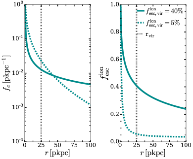
Figure 1.— Left panel: Radial profiles of neutral gas covering factor, which denotes the number of self-shielding clumps along a differential length at a distance $r$ from the central galaxy. Right panel: Profiles for the escape fraction of ionizing photons, i.e., the fraction of the total number of photons reaching a distance $r$ without being absorbed or destroyed. The solid and dashed dark cyan lines represent the two CGM models, parametrized accounting for the value of the escape fraction at the virial radius (denoted as dashed vertical line).

2.1.1 Central Galaxy, $C$ and $\dot{n}_{\rm ion}(r)$

We consider a $5L^{*}$ galaxy at $z=6.17$ for our calculations, which corresponds to $M_{\rm UV}\simeq-22.2$ adopting the fitting formula for $M^{*}$ from Kuhlen & Faucher-Giguère 2012 (their FIT model). We require a bright galaxy for the fluorescent component to dominate above the possible nebular satellite signal and avoid contamination, and at a level that can yield a good signal-to-noise ratio (S/N) for the observations. As we will show later, targeting fainter galaxies would require the stack of several objects or averaging the signal in larger radial bin sizes in order to obtain reasonable S/N. However, brighter galaxies are rare, and the probability of finding one in the field of view (FOV) considered in our calculations becomes undesirably small (see § 3.2.1). The conversion factor between UV luminosity and star formation rate (SFR) for high redshift by Madau & Dickinson (2014),

$$L_{\rm UV}{\rm[erg\,s^{-1}\,Hz^{-1}]}=8.7\times 10^{27}\,{\rm SFR}\,{\rm[M_{\odot}\,yr^{-1}]}~{},$$ (3)

yields a SFR $\sim 41.4\,{\rm M_{\odot}\,yr^{-1}}$ for the central galaxy. We have not considered additional dust attenuation for this calculation because we expect the effect of dust at these redshifts to be low (see section 3.1.3 in Madau & Dickinson, 2014, for further discussion). This assumption results in a lower limit for the SFR and, in turn, for the surface brightness which depends linearly on SFR.

The SFR then determines the total production rate of ionizing photons as (Robertson et al., 2013),

$$\dot{N}_{\rm ion}\,{\rm[photons\,s^{-1}]}=1.38\times 10^{53}\,{\rm SFR\,[M_{\odot}\,yr^{-1}]}~{},$$ (4)

which we use to compute $n_{\rm ion}(r)$ as

$$\dot{n}_{\rm ion}(r)=\frac{\dot{N}_{\rm ion}}{4\pi r^{2}}~{}.$$ (5)

We assume that each ionizing photon is converted into H$\alpha$ and Ly$\alpha$ with an efficiency that is set by case-B recombination. Under this assumption, the parameter $C$ for Ly$\alpha$ and H$\alpha$ is

$$C\,{\rm[erg\,sr^{-1}]}=\frac{1}{4\pi}\,\frac{\alpha_{\rm X}^{\rm eff}}{\alpha_{\rm B}}\,h\nu_{X}~{}.$$ (6)

The fraction $\alpha_{\rm X}^{\rm eff}/\alpha_{\rm B}$ denotes the number of line photons per ionizing photon (X takes on ‘H$\alpha$’ or ‘Ly$\alpha$’), and equals $0.68$ for Ly$\alpha$ and $0.45$ for H$\alpha$. In detail, both the production rate of ionizing photons and the conversion efficiency into H$\alpha$ and Ly$\alpha$ line photons depend on the IMF, metallicity, stellar populations, etc., at these redshifts (Raiter et al., 2010; Mas-Ribas et al., 2016, see also the discussion in Mas-Ribas et al. 2017). The factors $h\nu_{X}$ and $1/4\pi$ account for the energy and isotropic emission of the line photons, respectively.

2.1.2 CGM, $f_{c}(r)$ and $f_{\rm esc}^{\rm ion}(r)$

The characteristics of the CGM at the redshifts of reionization are not known. We parametrize our ignorance by considering the two most extreme CGM models at $z=3.1$ developed in Mas-Ribas & Dijkstra (2016). In these models, the CGM is composed of a spherically symmetric distribution of neutral hydrogen clumps embedded within a hot medium. The distribution of clumps is characterized by the cold gas covering fraction, $f_{c}(r)$, which denotes the number of neutral clumps along a differential length, at a distance $r$ from the central galaxy. The escape fraction of ionizing photons is distance dependent in our models, and relates to the covering fraction as $f_{\rm esc}^{\rm ion}(r)={\rm exp}[-\int_{0}^{r}f_{c}(r){\rm d}r]$. To stress, this parameter represents the escape fraction of ionizing photons out to a distance $r$. Our calculations assume a $100\%$ escape fraction at $r=0$, but our results scale linearly with this value. We parametrize the two CGM models using the value of the escape fraction of ionizing photons at the virial radius of the central galaxy ($\sim 25$ pkpc, for a dark matter halo $M_{h}\sim 1.5\times 10^{11}\,{\rm M_{\odot}}$), and describe them below:

1. $f_{\rm esc,vir}^{\rm ion}=40\%$: This CGM model derives from that proposed by Steidel et al. (2010), where the neutral hydrogen clumps are in pressure equilibrium with a radially accelerating outflowing hot medium. The dark cyan solid lines in the left and right panels of Figure 1 display the gas covering factor and ionizing escape fraction profiles, respectively. This model produces an escape fraction at the virial radius of $40\%$.

2. $f_{\rm esc,vir}^{\rm ion}=5\%$: This CGM model is obtained after applying an inverse Abelian transformation to the two-dimensional neutral hydrogen covering factor from the simulations by Rahmati et al. (2015), in order to obtain a radial dependent covering factor (see Mas-Ribas & Dijkstra 2016 for this transformation). The corresponding profiles are represented by the dashed dark cyan lines in the left and right panels of Figure 1. The escape fraction in this model reaches a value $\sim 5\%$ at the virial radius.

Figure 1 shows that the radial dependence of the escape fraction is mostly driven by the covering factor profile in the first $\sim 50$ pkpc from the central galaxy. The left panel shows that the covering factor in the $f_{\rm esc,vir}^{\rm ion}=40\%$ model is smaller at those distances, which yields a smoother decrease of the ionizing escape fraction in this case. Conversely, the escape fraction profile for the $f_{\rm esc,vir}^{\rm ion}=5\%$ model reaches a low value rapidly at $r\sim 25$ pkpc since the covering fraction decreases slowly with radial distance.

2.2. Surface Brightness from Satellite Sources:
Nebular radiation

We calculate the Ly$\alpha$ and H$\alpha$ surface brightness of the satellite sources as in Mas-Ribas et al. (2017),

$$SB^{\rm sat}(b)=\frac{2}{(1+z)^{4}}\int_{b}^{\infty}\epsilon_{X}[1+\xi_{X}(r)]f_{\rm esc,X}\,\frac{r{\rm d}r}{\sqrt{r^{2}-b^{2}}}~{},$$ (7)

where $\epsilon_{X}$ refers to the average cosmic emissivity for Ly$\alpha$ or H$\alpha$ (see § 2.2.1), $\xi_{X}$ is the correlation function for the corresponding radiation (see § 2.2.2), and $f_{\rm esc,X}$ denotes the escape fraction from the satellites for the transition ${\rm X}$. We (arbitrarily) set a fiducial value $f_{\rm esc,X}=40\%$, but also explore the broad ranges $0.2\geq f_{\rm esc,X}\geq 0.7$ and $0.1\geq f_{\rm esc,X}\geq 1.0$, because the escape fraction is not known at these high redshifts, especially for faint satellite sources, and is linked to the uncertain presence of dust, which likely affects more the Ly$\alpha$ photons than those of H$\alpha$ due to radiative transfer effects and the frequency dependence of the attenuation curve. We again limit the integral to 100 pkpc, and enable the presence of satellites at distances above 10 pkpc.

In addition to nebular Ly$\alpha$ and H$\alpha$ radiation, the satellite sources will also produce continuum radiation associated to star formation, which will result in an overall extended continuum profile. We calculate the visible (rest-frame, VIS) continuum surface brightness profile from that of H$\alpha$ as

$$SB_{\rm VIS}(b)=\frac{(1+z)}{\rm EW_{H\alpha}}\frac{\lambda_{\rm H{\alpha}}^{2}}{c}\,SB_{\rm H\alpha}^{\rm sat}(b)~{}.$$ (8)

We assume a fiducial H$\alpha$ line equivalent width (rest-frame) ${\rm EW_{H\alpha}=300\,\,{\rm\AA}}$, considering the observations by Mármol-Queraltó et al. 2016 (and references therein), and also explore the ranges $450\geq{\rm EW_{H\alpha}\,(\AA)\geq 150}$ and $700\geq{\rm EW_{H\alpha}\,(\AA)\geq 50}$. The parameters $\lambda_{\rm H\alpha}$ and $c$ denote the rest-frame H$\alpha$ wavelength and the speed of light, respectively and, combined with the term $(1+z)$, yield a surface brightness per unit frequency.

2.2.1 Emissivity, $\epsilon$

To obtain the average H$\alpha$ cosmic emissivity for the satellite population, we calculate the cosmic SFR density at the redshift of interest using equation 2 in Robertson et al. (2015), which considers radiation from sources down to $M_{\rm UV}\sim-13$, and assume that the SFR for the satellites equals this value. In reality, the SFR for the satellites will be a fraction of total cosmic star formation, but its value is unknown and degenerate with the escape fraction of H$\alpha$ photons (e.g., Trenti et al., 2012). We finally use the relation by Kennicutt & Evans (2012),

$$L_{\rm H\alpha}\,{\rm[erg\,s^{-1}]}=1.86\times 10^{41}\,{\rm SFR\,[M_{\odot}\,yr^{-1}]}~{},$$ (9)

to obtain the average volumetric emissivity for H$\alpha$ radiation. We consider that the emissivity for Ly$\alpha$ will simply be a factor $8.1$ higher, which is the proper intrinsic ratio between the volume emissivities for Ly$\alpha$ and H$\alpha$ computed from the tables in Osterbrock (1989), consistent with the approach adopted in Eq. 6, and noting again the dependence of this value on dust content.

2.2.2 Clustering, $\xi(r)$

We adopt a power-law two-point correlation function for the clustering of satellite sources around the bright central galaxy, with correlation length $r_{0}=3.79\,{\rm Mpc\,h^{-1}}$ and power-law index $\alpha=-1.8$, as reported by Harikane et al. (2016), for their sample of LBG galaxies with average magnitude $\langle M_{\rm UV}\rangle=-19.3$ at $z=5.9$. In Mas-Ribas et al. (2017) we used another clustering prescription because, at small distances, the departures from a power-law by the data of Ouchi et al. (2010) at $z=3.1$ were significant. In the current case, however, the power-law approach is consistent within 1$\sigma$ with the data by Harikane et al. (2016), which extend up to $\sim 12$ pkpc from the central galaxy. We consider the same bias for the H$\alpha$ radiation and the satellite sources because radiative transfer effects, i.e., scattering, are not present for the case of H$\alpha$ (Mas-Ribas et al., 2017). We adopt these same values for the satellite clustering when comparing with the LAE data by Momose et al. (2014) and Jiang et al. (2013), owing to the broad range of uncertainties and overlap of values between the correlation lengths from $z=5.7$ to $z=6.8$ in the different data samples of LAEs and LBGs in Ouchi et al. (2010) and Harikane et al. (2016), respectively. Possible variations of the clustering of sources and/or radiation are engulfed in the large range explored for the escape fraction described above.

3. Results

We present below our results. In § 3.1, we apply and compare our analytical models to the observational Ly$\alpha$ data by Momose et al. (2014) and Jiang et al. (2013) at $z=5.7$ and $z=6.6$. In § 3.2, we detail a potential JWST observational strategy (§ 3.2.1), and present the predicted H$\alpha$ and VIS continuum surface brightness profiles at $z=6.17$ (§ 3.2.2).

3.1. Ly$\alpha$

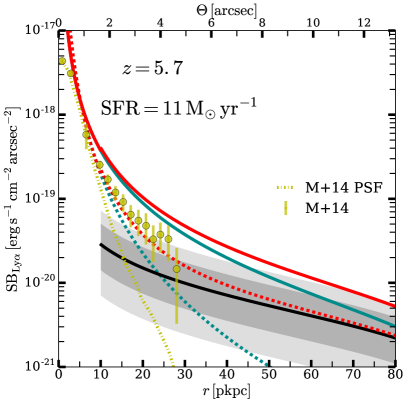
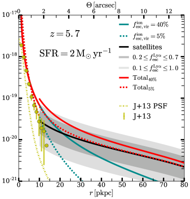
Figure 2.— Comparison between our predicted Ly$\alpha$ surface brightness profiles and the observational data by Momose et al. 2014 (their mean values, M+14, left panel) and Jiang et al. 2013 (J+13, right panel) at $z=5.7$. The yellow points with uncertainties denote the observed profiles and the yellow dashed lines the PSFs. The profiles of the $f_{\rm esc,vir}^{\rm ion}=40\%$ ($f_{\rm esc,vir}^{\rm ion}=5\%$) CGM models are displayed as the solid (dashed) dark cyan lines. The solid black line and shaded grey bands represent the fiducial model for the profiles of the satellites and the different escape fraction ranges, respectively. The solid (dashed) red lines denote the total (central + satellite) profiles for the $40\%$ ($5\%$) CGM models. The SFRs for the central galaxies are quoted in every panel. In general, the low escape fraction models result in a better match to both data sets, although the contribution of satellites is unclear (see text).

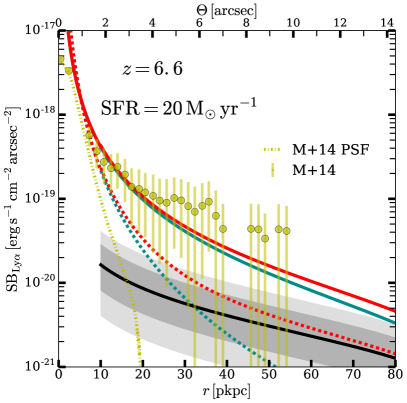
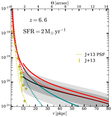
Figure 3.— Same as Figure 2 but at $z=6.6$. In this case, the data by Momose et al. (2014) seems to be better matched by the model with high ionizing escape fraction, although the error bars are consistent with the two CGM models within 1$\sigma$ for most of the data points, and the possibility for the presence of artifacts in the observations is elevated (see text). As at $z=5.7$, the data by Jiang et al. (2013) favors the low escape fraction model and discards the contribution from satellites.

Figures 2 and 3 display the comparison between our predicted Ly$\alpha$ surface brightness profiles and the observational data at $z=5.7$ and $z=6.6$, respectively, by Momose et al. 2014 (their mean values, left panels) and Jiang et al. 2013 (right panels). The yellow data points and error bars denote the data and uncertainties, and the yellow dashed lines the point-spread functions (PSFs) quoted by these authors. In general, the data by Momose et al. show significant extended emission well beyond the PSF. Jiang et al. argue that the extended emission in their observations is due to the fact that the central galaxy is resolved, but not to the presence of an extended halo. The Ly$\alpha$ data by Jiang et al. corresponds to the stack of 43 (40) LAEs at $z=5.7$ ($z=6.6$), a subsample selected from the observations by Ouchi et al. (2008, 2010); Kashikawa et al. (2011), reaching a surface brightness limit $\sim 1.2\times 10^{-19}\,{\rm erg\,s^{-1}\,{\rm cm}^{-2}\,arcsec^{-2}}$. The stacked profiles in Momose et al. arise from 397 (119) LAEs at $z=5.7$ ($z=6.6$), selected from the parent sample of observations by Ouchi et al. (2008, 2010), and reach similar (within a factor $\sim 2$) Ly$\alpha$ surface brightness limits compared to the Jiang et al. data. The two datasets of overlapping (but different) galaxy samples do not agree with each other; Momose et al. attributes the lack of extended emission in the analysis by Jiang et al. to the small sample size.

To obtain consistent comparisons, we calculate the star formation rates for the central galaxy in the observed data sets as follows: We integrate the corresponding UV continuum surface brightness profiles by Momose et al. 2014 (their figure 3) to calculate the UV luminosity and then use Eq. 3 to obtain the SFRs. Since the UV surface brightness profiles or galaxy sample are not available in Jiang et al. (2013), we calculate the ratio between the integrated Ly$\alpha$ surface brightness profiles in the inner regions, where the central galaxy dominates, in Momose et al. (2014) and Jiang et al. (2013), and assume these Ly$\alpha$ ratios to be the same as for the SFRs. At $z=5.7$, integrating up to a distance of 4 (1) arcsec, the ratio is $\sim 5.5$ ($\sim 4$). At $z=6.6$, the same upper limits for the integral result in ratios $\sim 12.8$ and $\sim 6.6$, respectively. For simplicity, we set the ratios to 5.5 and 10 at $z=5.7$ and $z=6.6$, respectively, and stress that the results depend linearly on these parameters.

The dark cyan solid (dashed) lines in Figures 2 and 3 denote the surface brightness profiles for the $f_{\rm esc,vir}^{\rm ion}=40\%$ ($f_{\rm esc,vir}^{\rm ion}=5\%$) CGM models, with the SFR of the central galaxy quoted in each panel. The black lines and shaded grey areas represent the profiles for the fiducial model and the two ranges of nebular radiation escape fraction, respectively, for the satellite sources. The red solid (dashed) lines represent the total, central + satellite galaxies, surface brightness profiles for the $40\%$ ($5\%$) CGM models.

At $z=5.7$ (Figure 2), both data sets are better matched by the low escape fraction CGM model, despite the factor $5.5$ between the respective SFRs. The contribution of satellites appears, however, unclear: For the Jiang et al. data (right panel), the match to the observations is the best when satellites are ignored while, for the Momose et al. case (left panel), the satellites provide the necessary signal to reach the observed values at distances $r\gtrsim 15$ pkpc.

At $z=6.6$ (Figure 3), the data by Jiang et al. (right panel) is better reproduced by the low escape fraction CGM model again but, contrary to the previous findings, for the Momose et al. data (left panel), even the high escape fraction model lies below the observations in this case, and the contribution of the satellite sources is not enough to approach the observed levels. However, the uncertainties in the data by Momose et al. here are significantly large, resulting in the low escape fraction model being at a $\lesssim 1\sigma$ level for most of the data points. The high observed profile might be a consequence of the high star formation rate, ${\rm SFR\sim 20\,M_{\odot}\,yr^{-1}}$, but it is more likely that the observations below $\sim 1-2\times 10^{-19}\,{\rm erg\,s^{-1}\,{\rm cm}^{-2}\,arcsec^{-2}}$ are mostly driven by systematic effects, as tested by Momose et al. 2014 (their section 3.2 and figure 8).

Taking into account the possible systematic effects in the data by Momose et al. (2014) at $z=6.6$, the low ionizing escape fraction CGM model, $f_{\rm esc,vir}^{\rm ion}=5\%$, seems to be the most consistent one with the observed Ly$\alpha$ profiles in general, regardless the average SFR values for the central galaxies, which cover the corresponding magnitude range $-19\gtrsim M_{\rm UV}\gtrsim-21.5$. If this result is confirmed, these galaxies would not have contributed significantly to the reionization process, and a large population of fainter galaxies with a high ionizing escape fraction would be necessary. However, the presence of satellite sources is never required by the data in Jiang et al. (2013), and only at distances $r\gtrsim 15-20$ physical kpc from the central galaxy by the observations of Momose et al. (2014), where the uncertainties and possible systematic effects are important. The apparent discrepancy between the two different data-sets prevents us from drawing firm conclusions. We present below the H$\alpha$ and visual continuum predicted profiles and JWST observations, which will constitute additional probes, and will further extend this discussion in § 4.

3.2. H$\alpha$ and VIS

We present below the predicted H$\alpha$ and visible (VIS) continuum surface brightness profiles (§ 3.2.2), and the approach we adopt for future JWST observations of these extended halos (§ 3.2.1). Contrary to Ly$\alpha$, the H$\alpha$ transition is not resonant, implying that the H$\alpha$ photons do not scatter the neutral hydrogen gas. This characteristic facilitates the interpretation of the H$\alpha$ profiles compared to those of Ly$\alpha$: H$\alpha$ photons, either come from star formation or fluorescence, thus tracing their production sites.

3.2.1 H$\alpha$ & VIS: JWST Observational Strategy

We consider the near infrared camera, NIRCam, instrument onboard JWST for our observations, with a field of view ${\rm FOV=9.68}\,{\rm arcmin^{2}}$. We perform the calculations at $z=6.17$ for the H$\alpha$ radiation to match the position of the F470N narrow-band (NB) filter, with a band width (BW) ${\rm BW=0.051\,\mu}$m, and centered at $4.708\,\mu$m observer-frame. For the visible continuum, we adopt the filter F410M, with ${\rm BW=0.438\,\mu}$m, and centered at $4.082\,\mu$m, corresponding to a rest-frame wavelength $\sim 5693\,{\rm\AA}$. In both cases, we consider a total observing time $t_{\rm exp}=10^{5}$ s. We compute the sky background at $4.708\,\mu$m following the technical note http://www.stsci.edu/~tumlinso/nrs_sens_2852.pdf (Eq. 22), resulting in a surface brightness $SB_{\rm sky}=6\,\mu{\rm Jy\,arcsec^{-2}\,(\sim 22\,mag\,arcsec^{-2})}$.

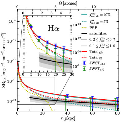
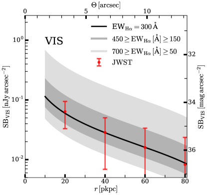
Figure 4.— Left panel: Radial surface brightness profiles with physical distance for one $5L^{*}$ galaxy. The solid (dashed) dark cyan lines denote the H$\alpha$ profiles of the $f_{\rm esc,vir}^{\rm ion}=40\%$ ($f_{\rm esc,vir}^{\rm ion}=5\%$) CGM models. The black line represents the profile from the satellite sources considering $f_{\rm esc}^{\rm H\alpha}=40\%$, while the grey shaded areas denote the ranges $0.2\geq f_{\rm esc}^{\rm H\alpha}\geq 0.7$ and $0.1\geq f_{\rm esc}^{\rm H\alpha}\geq 1.0$. The solid (dashed) red line denotes the total (central + satellite) profile for the $40\%$ ($5\%$) CGM model, and the blue and green data points with their uncertainty, are the predicted corresponding JWST observations for these total profiles. The inset figure zooms in the inner $r\leq 30$ pkpc. The green vertical lines denoting uncertainties in the observations are slightly shifted from the original position to facilitate the visualization. Right panel: Radial visible (VIS) continuum profile due to the satellite sources, obtained after stacking the images of $\sim 18\,L>0.1L^{*}$ galaxies detected in one NIRCam pointing. The black solid line denotes the fiducial model (${\rm EW_{H\alpha}=300\,\,{\rm\AA}}$), and the shaded regions the equivalent width ranges $450\geq{\rm EW_{H\alpha}\,(\AA)\geq 150}$ and $700\geq{\rm EW_{H\alpha}\,(\AA)\geq 50}$. The observations and uncertainties are displayed in red.

Following Mas-Ribas et al. 2017 (Appendix B), we derive the uncertainties in the observations from the signal-to-noise ratio (S/N), computed as ${\rm S/N}=N_{s}/\sqrt{N_{s}+N_{\rm sky}}$, where $N_{s}$ and $N_{\rm sky}$ are the azimuthally integrated source and sky photon number counts, respectively, defined as

$$N_{s} = \frac{f_{\rm H\alpha}}{h\,\nu_{\rm H\alpha}^{\rm obs}}\,{\rm A_{aper}}\,\eta\,t_{\rm exp}~{},$$ (10)

$$N_{\rm sky} = \frac{f_{\rm sky}}{h\,\nu_{\rm H\alpha}^{\rm obs}}\,{\rm BW}\,{\rm A_{aper}}\,\eta\,t_{\rm exp}~{}.$$ (11)

The aperture for JWST is ${\rm A_{aper}=25\,m^{2}}$, and $\eta=0.469\,(0.274)$ is the total system throughput for the continuum (line) filter. The terms ${f_{\rm H\alpha}}$ and ${f_{\rm sky}}$ are the source and sky fluxes, respectively, resulting from the integration of the surface brightness over the area of the corresponding radial annulus around the central galaxy, and ${h\nu_{\rm H\alpha}^{\rm obs}}$ denotes the H$\alpha$ photon energy at the observer frame, $z=6.17$. We include the term BW in the sky background and VIS calculations because the sky and continuum are in units of flux density. We have not accounted for other systematics or noise effects in this simple calculation but we have checked that our S/N results are in broad agreement with those produced using the JWST on-line Time Exposure Calculator (ETC).

We obtain the profile driven by the PSF as follows: We compute the encircled energy (EE) radial profile for the narrow band F470N filter with the publicly available package WebbPSF, and convolve it with the total H$\alpha$ luminosity produced by the central galaxy, assumed to be a point source. We plot the resulting PSF profile as the yellow dashed line in Figure 4, after applying the luminosity distance and geometric factors to transform the luminosity into surface brightness.

To obtain a high S/N for the H$\alpha$ profiles, it would be desirable to observe the brightest possible galaxies, $L~{}\hbox to0.0pt{$>$\hss}{\lower 4.30554pt\hbox{$\sim$}}10L^{*}$, but these objects are sufficiently rare that it is unlikely to find one in a single JWST NIRCam pointing (observation). Fainter objects, $L\sim L^{*}$, result in larger number densities but, in this case, the signal from possible satellites easily overcomes that of the central galaxy, contaminating the escape fraction measurements. In addition, the stacking of a large number of these objects would be required to reach a good S/N, introducing possible systematics from the complex stacking methodology, and increasing the number of JWST pointings, i.e., observing time. We consider the case of observing one $5L^{*}$ galaxy previously detected by a wide-field spectroscopic or NB imaging survey covering an area in the sky of 10 deg². We adopt these numbers as a compromise between the number of $5L^{*}$ objects in the volume adopted, $\sim 2$ when integrating the UV luminosity function at $z=6.17$ with the parameters from the fitting formula by Kuhlen & Faucher-Giguère 2012 ($M_{\rm UV}^{*}=-20.374$, $\phi^{*}=9.5\times 10^{\rm-4}\,{\rm Mpc^{-3}\,mag^{-1}}$, and $\alpha=-1.85$), the required observing time, and the S/N.

The signal from the satellite sources is independent of the brightness of the central galaxy, assuming that the clustering is similar for a range of galaxy luminosities. We consider the stacked image of $\sim 18\,L>0.1L^{*}\,(M_{\rm{UV}}<-18)$ galaxies for the calculation of the visible continuum observation, which is the number of objects present in the NIRCam FOV (a single pointing).

3.2.2 H$\alpha$ & VIS: Predicted Surface Brightness Profiles

We present the resulting H$\alpha$ and continuum surface brightness profiles, considering one $5L^{*}$ and eighteen $L>0.1L^{*}$ galaxies, respectively, at $z=6.17$. The analysis of the continuum will be useful to probe the satellite contribution for both, assessing their existence and separating their contribution from that of the central galaxy. The left panel in Figure 4 displays the surface brightness profiles for H$\alpha$, where the dark cyan solid (dashed) line denotes the predictions for the $f_{\rm esc,vir}^{\rm ion}=40\%$ ($f_{\rm esc,vir}^{\rm ion}=5\%$) CGM model for the central galaxy. The black line represents the fiducial profile for the satellite sources at $r\geq 10$ pkpc, considering $f_{\rm esc}^{\rm H\alpha}=40\%$, and the grey shaded areas represent the ranges $0.2\geq f_{\rm esc}^{\rm H\alpha}\geq 0.7$ and $0.1\geq f_{\rm esc}^{\rm H\alpha}\geq 1.0$. The solid (dashed) red line denotes the total (central + satellites) profile for the $40\%$ ($5\%$) CGM model, and the blue and green error bars represent the uncertainties in the JWST observations described in the previous section for the corresponding total profiles. The yellow dashed line denotes the PSF profile. The inset figure zooms into the range $5\lesssim r\lesssim 30$ pkpc. The right panel shows the surface brightness profiles and observations of the visible continuum from the satellite galaxies, for the fiducial model (${\rm EW_{H\alpha}=300\,\,{\rm\AA}}$), and the equivalent width ranges $450\geq{\rm EW_{H\alpha}\,(\AA)\geq 150}$ and $700\geq{\rm EW_{H\alpha}\,(\AA)\geq 50}$. The red data and error bars denote the JWST observations, which present detections up to $\sim 40$ pkpc from the center of the galaxy.

The left panel in Figure 4 indicates that JWST observations will be able to probe the surface brightness profiles up to distances $r\sim 50$ pkpc for the case of the $f_{\rm esc}^{\rm ion}\sim 40\%$ model. These observations would imply that a significant fraction of the ionizing radiation from galaxies reaches large distances from the center, contributing to the reionization of the intergalactic medium (IGM). Instead, a low ionizing escape fraction similar to the $f_{\rm esc}^{\rm ion}\sim 5\%$ model, results in a profile detectable up to $r\sim 15$ pkpc. This result would indicate that most of the ionizing radiation does not escape beyond the CGM, thus not contributing significantly to cosmic reionization.

The fluorescent profile of the central galaxies, especially for the low ionizing escape fraction cases, might be contaminated by the PSF and the nebular radiation from the satellite sources. Observations of the VIS continuum profile will contribute differentiating between the two processes. A steep (almost non-existent) continuum profile beyond the central galaxy would imply that satellite radiation (and sources) are not important, and the extended profiles are driven by fluorescence. Conversely, an extended continuum signal would imply the presence of star formation (satellite sources) in the halo of the central galaxy, and would allow for the investigation of the nature and contribution of these faint source population to reionization. It is likely that the faint sources are too faint to be individually detected but their collective emission would produce the observable predicted profile, resembling the intensity mapping methodology. The right panel in Figure 4, however, demonstrates that the observation and stacking of several sources is necessary to obtain high S/N and differentiate between the different escape fraction scenarios for the satellite sources. Alternatively, larger radial bins sizes than the ones adopted here would provide higher S/N values at the cost of spatial resolution.

4. Discussion and Conclusion

We have proposed that extended emission around galaxies at $z\sim 6$ can be used to constrain the escape fraction of the ionizing radiation and/or the presence of faint satellite galaxies during the late stages of cosmic reionization. We have predicted radial surface brightness profiles which include the contribution from (i) fluorescent emission powered by ionizing radiation leaking from the central galaxy (as in Mas-Ribas & Dijkstra, 2016, for two different CGM prescriptions), and (ii), nebular emission from faint satellite sources that possibly resided within the halo of the central galaxies (as in Mas-Ribas et al., 2017). We have compared our predictions with observations of Ly$\alpha$ halos at $z=5.7$ and $z=6.6$, and have also predicted H$\alpha$ and visible continuum surface brightness profiles which may be detectable within future JWST observations.

We present and discuss our findings below:

• Our comparison of models to observations favors the model with a very low escape fraction of ionizing radiation, $f_{\rm esc}^{\rm ion}\sim 5\%$, from galaxies within the range of magnitudes $-19\gtrsim M_{\rm UV}\gtrsim-21.5$. This scenario implies that these galaxies do not contribute significantly to the reionization process. Therefore, if galaxies are the major contributors to the reionization process, as recently restated by Parsa et al. (2017), a large population of faint sources with a high ionizing escape fraction is necessary.

• The presence of faint satellite sources is unclear. Two out of four comparisons with current Ly$\alpha$ data indicate that satellite sources might contribute to the extended Ly$\alpha$ emission, but the effect of systematics and uncertainties in the observations do not allow for a clear conclusion. Given the required existence of faint sources driven by the low escape fraction results, if the presence of satellite sources around brighter galaxies is ruled out by the observations, this might imply that the population of faint objects is spread out within the intergalactic medium, making its detection more challenging.

• JWST will be able to probe the ionizing escape fraction from one bright, $L~{}\hbox to0.0pt{$>$\hss}{\lower 4.30554pt\hbox{$\sim$}}5L^{*}$, galaxy up to distances of a few tens of pkpc from the center. Fainter galaxies and/or a high signal-to-noise ratio for the continuum observations require the observation and stacking of several objects.

We stress that we have adopted and extrapolated two CGM models that were derived to match observables at redshifts around $z\sim 3$. The validity of our results, therefore, depends on the ability of these two models to realistically describe the medium surrounding $z\sim 6$ galaxies. While a more detailed parametrization of the CGM at high redshift (if currently feasible) is beyond the scope of our work, future observations of extended emission together with absorption studies (e.g., Dijkstra & Kramer, 2012; Hennawi & Prochaska, 2013; Prochaska et al., 2013, see also Steidel et al. 2010, 2011) will clearly enable us to use our proposed method to further constrain the escape fraction.

The prospects for doing this experiment at lower redshifts, $z\sim 3-4$, are interesting as the surface brightness for emission lines depends on redshift as $(1+z)^{4}$. However, the contribution from satellites can be more important at these low redshifts and overlap with the signal from the central galaxy (Mas-Ribas et al., 2017). At $z\sim 3.5$, we may be also benefiting from the observations by HETDEX (Hill et al., 2008) or MUSE (Bacon et al., 2014), for constraints on Ly$\alpha$ halos. While the escape fraction of ionizing photons at $z\sim 3.5$ is not directly relevant for reionization, using our approach may provide new insights for constraining $f_{\rm esc}^{\rm ion}$ and, in turn, the physical properties of the circumgalactic medium.

References

- Bacon et al. (2014) Bacon, R., Vernet, J., Borisova, E., et al. 2014, The Messenger, 157, 13
- Bouwens et al. (2015) Bouwens, R. J., Illingworth, G. D., Oesch, P. A., et al. 2015, ApJ, 803, 34
- Cantalupo et al. (2008) Cantalupo, S., Porciani, C., & Lilly, S. J. 2008, ApJ, 672, 48
- Dijkstra et al. (2016) Dijkstra, M., Gronke, M., & Venkatesan, A. 2016, ApJ, 828, 71
- Dijkstra & Kramer (2012) Dijkstra, M., & Kramer, R. 2012, MNRAS, 424, 1672
- Dijkstra & Loeb (2009) Dijkstra, M., & Loeb, A. 2009, MNRAS, 400, 1109
- Faucher-Giguère et al. (2010) Faucher-Giguère, C.-A., Kereš, D., Dijkstra, M., Hernquist, L., & Zaldarriaga, M. 2010, ApJ, 725, 633
- Feldmeier et al. (2013) Feldmeier, J. J., Hagen, A., Ciardullo, R., et al. 2013, ApJ, 776, 75
- Fonseca et al. (2017) Fonseca, J., Silva, M. B., Santos, M. G., & Cooray, A. 2017, MNRAS, 464, 1948
- Gardner et al. (2006) Gardner, J. P., Mather, J. C., Clampin, M., et al. 2006, Space Sci. Rev., 123, 485
- Goerdt et al. (2010) Goerdt, T., Dekel, A., Sternberg, A., et al. 2010, MNRAS, 407, 613
- Haiman et al. (2000) Haiman, Z., Spaans, M., & Quataert, E. 2000, ApJL, 537, L5
- Harikane et al. (2016) Harikane, Y., Ouchi, M., Ono, Y., et al. 2016, ApJ, 821, 123
- Hayes et al. (2013) Hayes, M., Östlin, G., Schaerer, D., et al. 2013, ApJL, 765, L27
- Hennawi & Prochaska (2013) Hennawi, J. F., & Prochaska, J. X. 2013, ApJ, 766, 58
- Hill et al. (2008) Hill, G. J., Gebhardt, K., Komatsu, E., et al. 2008, in Astronomical Society of the Pacific Conference Series, Vol. 399, Panoramic Views of Galaxy Formation and Evolution, ed. T. Kodama, T. Yamada, & K. Aoki, 115
- Jiang et al. (2013) Jiang, L., Egami, E., Fan, X., et al. 2013, ApJ, 773, 153
- Jones et al. (2012) Jones, T., Stark, D. P., & Ellis, R. S. 2012, ApJ, 751, 51
- Kashikawa et al. (2011) Kashikawa, N., Shimasaku, K., Matsuda, Y., et al. 2011, ApJ, 734, 119
- Kennicutt & Evans (2012) Kennicutt, R. C., & Evans, N. J. 2012, ARAA, 50, 531
- Kistler et al. (2009) Kistler, M. D., Yüksel, H., Beacom, J. F., Hopkins, A. M., & Wyithe, J. S. B. 2009, ApJL, 705, L104
- Kistler et al. (2013) Kistler, M. D., Yuksel, H., & Hopkins, A. M. 2013, ArXiv e-prints, arXiv:1305.1630
- Kuhlen & Faucher-Giguère (2012) Kuhlen, M., & Faucher-Giguère, C.-A. 2012, MNRAS, 423, 862
- Lake et al. (2015) Lake, E., Zheng, Z., Cen, R., et al. 2015, ArXiv e-prints, arXiv:1502.01349
- Laursen & Sommer-Larsen (2007) Laursen, P., & Sommer-Larsen, J. 2007, ApJL, 657, L69
- Leethochawalit et al. (2016) Leethochawalit, N., Jones, T. A., Ellis, R. S., Stark, D. P., & Zitrin, A. 2016, ApJ, 831, 152
- Madau & Dickinson (2014) Madau, P., & Dickinson, M. 2014, ARAA, 52, 415
- Mármol-Queraltó et al. (2016) Mármol-Queraltó, E., McLure, R. J., Cullen, F., et al. 2016, MNRAS, 460, 3587
- Mas-Ribas & Dijkstra (2016) Mas-Ribas, L., & Dijkstra, M. 2016, ApJ, 822, 84
- Mas-Ribas et al. (2016) Mas-Ribas, L., Dijkstra, M., & Forero-Romero, J. E. 2016, ApJ, 833, 65
- Mas-Ribas et al. (2017) Mas-Ribas, L., Dijkstra, M., Hennawi, J. F., et al. 2017, ApJ, 841, 19
- Matsuda et al. (2012) Matsuda, Y., Yamada, T., Hayashino, T., et al. 2012, MNRAS, 425, 878
- Matthee et al. (2016) Matthee, J., Sobral, D., Oteo, I., et al. 2016, MNRAS, 458, 449
- McCourt et al. (2016) McCourt, M., Oh, S. P., O’Leary, R. M., & Madigan, A.-M. 2016, ArXiv e-prints, arXiv:1610.01164
- Mitra et al. (2016) Mitra, S., Choudhury, T. R., & Ferrara, A. 2016, ArXiv e-prints, arXiv:1606.02719
- Momose et al. (2014) Momose, R., Ouchi, M., Nakajima, K., et al. 2014, MNRAS, 442, 110
- Osterbrock (1989) Osterbrock, D. E. 1989, Astrophysics of gaseous nebulae and active galactic nuclei
- Ouchi et al. (2008) Ouchi, M., Shimasaku, K., Akiyama, M., et al. 2008, ApJS, 176, 301
- Ouchi et al. (2010) Ouchi, M., Shimasaku, K., Furusawa, H., et al. 2010, ApJ, 723, 869
- Parsa et al. (2017) Parsa, S., Dunlop, J. S., & McLure, R. J. 2017, ArXiv e-prints, arXiv:1704.07750
- Prochaska et al. (2013) Prochaska, J. X., Hennawi, J. F., Lee, K.-G., et al. 2013, ApJ, 776, 136
- Rahmati et al. (2015) Rahmati, A., Schaye, J., Bower, R. G., et al. 2015, ArXiv e-prints, arXiv:1503.05553
- Raiter et al. (2010) Raiter, A., Schaerer, D., & Fosbury, R. A. E. 2010, A&A, 523, A64
- Reddy et al. (2016) Reddy, N. A., Steidel, C. C., Pettini, M., Bogosavljević, M., & Shapley, A. E. 2016, ApJ, 828, 108
- Robertson & Ellis (2012) Robertson, B. E., & Ellis, R. S. 2012, ApJ, 744, 95
- Robertson et al. (2015) Robertson, B. E., Ellis, R. S., Furlanetto, S. R., & Dunlop, J. S. 2015, ApJL, 802, L19
- Robertson et al. (2013) Robertson, B. E., Furlanetto, S. R., Schneider, E., et al. 2013, ApJ, 768, 71
- Rosdahl & Blaizot (2012) Rosdahl, J., & Blaizot, J. 2012, MNRAS, 423, 344
- Sobral et al. (2017) Sobral, D., Matthee, J., Best, P., et al. 2017, MNRAS, 466, 1242
- Steidel et al. (2011) Steidel, C. C., Bogosavljević, M., Shapley, A. E., et al. 2011, ApJ, 736, 160
- Steidel et al. (2010) Steidel, C. C., Erb, D. K., Shapley, A. E., et al. 2010, ApJ, 717, 289
- Sun & Furlanetto (2016) Sun, G., & Furlanetto, S. R. 2016, MNRAS, 460, 417
- Trenti et al. (2012) Trenti, M., Perna, R., Levesque, E. M., Shull, J. M., & Stocke, J. T. 2012, ApJL, 749, L38
- Trenti et al. (2010) Trenti, M., Stiavelli, M., Bouwens, R. J., et al. 2010, ApJL, 714, L202
- Verhamme et al. (2016) Verhamme, A., Orlitova, I., Schaerer, D., et al. 2016, ArXiv e-prints, arXiv:1609.03477
- Weisz & Boylan-Kolchin (2017) Weisz, D. R., & Boylan-Kolchin, M. 2017, ArXiv e-prints, arXiv:1702.06129
- Wisotzki et al. (2016) Wisotzki, L., Bacon, R., Blaizot, J., et al. 2016, A&A, 587, A98
- Xue et al. (2017) Xue, R., Lee, K.-S., Dey, A., et al. 2017, ApJ, 837, 172
- Yang et al. (2006) Yang, Y., Zabludoff, A. I., Davé, R., et al. 2006, ApJ, 640, 539
- Yue et al. (2016) Yue, B., Ferrara, A., & Xu, Y. 2016, MNRAS, 463, 1968
- Zackrisson et al. (2013) Zackrisson, E., Inoue, A. K., & Jensen, H. 2013, ApJ, 777, 39
- Zackrisson et al. (2016) Zackrisson, E., Binggeli, C., Finlator, K., et al. 2016, ArXiv e-prints, arXiv:1608.08217