How fast is mass-segregation happening in hierarchical formed embedded star clusters?

Abstract

We investigate the evolution of mass segregation in initially sub-structured young embedded star clusters with two different background potentials mimicking the gas. Our clusters are initially in virial or sub-virial global states and have different initial distributions for the most massive stars: randomly placed, initially mass segregated or even inverse segregation. By means of N-body simulation we follow their evolution for $5$ Myr. We measure the mass segregation using the minimum spanning tree method $\Lambda_{\rm MSR}$ and an equivalent restricted method. Despite this variety of different initial conditions, we find that our stellar distributions almost always settle very fast into a mass segregated and more spherical configuration, suggesting that once we see a spherical or nearly spherical embedded star cluster, we can be sure it is mass segregated no matter what the real initial conditions were. We, furthermore, report under which circumstances this process can be more rapid or delayed, respectively.

1 Introduction

Mass segregation (MS) has been detected in embedded star clusters (Lada et al., 1996; Hillenbrand, 1997; Hillenbrand & Hartmann, 1998; Bonatto & Bica, 2006; Chen et al., 2007; Er et al., 2013), i.e., that the most massive stars are more centrally concentrated. Advances in observations have shown that star clusters form sub-structured (Larson, 1995; Elmegreen, 2000; Testi et al., 2000; Williams, 2000; Cartwright & Whitworth, 2004; Gutermuth et al., 2005; Schmeja & Klessen, 2006; Carpenter & Hodapp, 2008; Schmeja et al., 2008) and this has also been supported by simulations (Klessen & Burkert, 2000, 2001; Bate et al., 2003; Bonnell et al., 2003; Bate, 2009; Offner et al., 2009; Girichidis et al., 2012; Dale et al., 2012). Observations also show that stars form dynamically cool (sub-virial state) (Peretto et al., 2006, 2007; Proszkow & Adams, 2009) and this property is supported by hydrodynamical simulations of star formation (Klessen & Burkert, 2000; Offner et al., 2009; Maschberger et al., 2010). A sub-virial initial state quickly erases primordial substructure, producing a smooth and more spherical cluster (Allison et al., 2009).

The process to form a segregated cluster can be dynamical (McMillan et al., 2007; Allison et al., 2009; Yu et al., 2011) and fast for cool and sub-structured clusters (Allison et al., 2010; Parker et al., 2016) reaching some level of MS in $\sim 1$ Myr. Primordial MS is also possible, as a result of the star formation process (Zinnecker, 1982; Murray & Lin, 1996; Elmegreen & Krakowski, 2001; Klessen, 2001a; Bonnell et al., 2001; Bonnell & Bate, 2006) where the massive stars tend to form in the centre of the star-forming regions because of higher accretion rates in the central parts or as a result of competitive accretion (Larson, 1982; Murray & Lin, 1996; Bonnell et al., 1997). The later has been used to explain very high levels of MS in very young objects, when dynamical processes are not fast enough to explain the observed MS (Bonnell & Davies, 1998; Raboud & Mermilliod, 1998). On the other hand Parker et al. (2015) pointed out that primordial mass segregation rarely occurs if massive stars form by competitive accretion.

In this paper, we show the evolution of MS for young embedded star clusters, which form hierarchical out of fractal initial distributions (similar to Parker et al., 2014), but under the influence of two different background (BG) potentials and their importance depending on the locations of the massive stars. We start our simulations after the end of the star formation process where the dynamics of the stars become important.

In Section 2 we present the method and the different initial conditions that we explore. We continue in Section 3 with the presentation of the results of our $N$-body simulations. In Section 4 we discuss our results focusing on the different evolution of MS depending on the initial conditions. We conclude in Section 5.

2 Method and Initial Conditions

2.1 Initial conditions of the stars

The stars are initially placed in a fractal distribution.

We use the method of Goodwin & Whitworth (2004) to generate initially sub-structured distributions. This method defines a cube of size $N_{\rm div}=2$ in which the fractal is created. This cube is the first-generation parent which is divided in $N^{3}_{\rm div}$ sub-cubes (in our case $N^{3}_{\rm div}=8$). Each sub-node, called child, can turn into a parent for a next generation with a probability of $N^{D-3}_{\rm div}$ where $D$ is the fractal dimension, for which we choose a $D=1.6$. The probability to become a parent is clearly ruled by the value of the fractal dimension. For lower values of $D$ less children turn into parents and so a more sub-structured distribution is produced. On the other hand, a value of $D=3$ corresponds to an uniform distribution. The not surviving children are removed, then a small noise (displacement from the centre of the cell of a few per cent of the cell-size) is added to the remaining survivals to prevent an artificial grid-like structure and finally they become parents for the next step. The mature children are divided into $N^{3}_{\rm div}$ new children of which again, using a probability of $N^{(D-3)}_{\rm div}$, become a parent. The process is repeated until the number of children reaches a larger number than the number of particles.

The velocities of the parents follow a Gaussian with a mean of zero and the children inherit the velocity from the parent including a random component that decreases with each new generation. That way stars in the same area or clump have similar velocities and are not flying in completely different directions. The velocities get later scaled to obtain the desired virial ratio (see further below).

We change the random seed value to produce different fractal distributions with a maximum radius of $1.5$ pc.

To the distribution of positions and velocities from the previous step we assign masses using the modified initial mass function of Kroupa (2002), following:

$$N(M) \varpropto \begin{cases}M^{-1.30}&\forall\ m_{0}\leq M/{\rm M}_{\odot}<m_{1}\\ M^{-2.30}&\forall\ m_{1}\leq M/{\rm M}_{\odot}<m_{2}\\ M^{-2.35}&\forall\ m_{2}\leq M/{\rm M}_{\odot}<m_{3}\end{cases}$$ (1)

with $m_{0}=0.08$, $m_{1}=0.5$, $m_{2}=1.0$, $m_{3}=50$ M_⊙. The distribution is modified in the sense that we avoid the sub-stellar mass range (below $0.08$ M_⊙ for brown dwarfs). The total mass of stars is $\sim 500$ M_⊙ for $\sim 1000$ stars which are common values for these kind of objects (Piskunov et al., 2008).

,

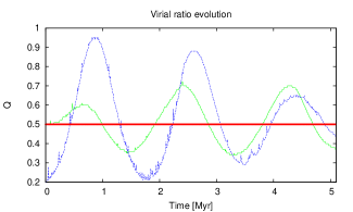
Figure 1: Example of the evolution of the virial ratio for a fractal distribution. The green solid line shows the oscillations for a fractal starting from a pseudo virial equilibrium ($Q_{\rm init}=0.5$) and the blue dashed line shows the changes for the same fractal now starting from a cool state ($Q_{\rm init}=0.2$). Horizontal line denotes the virial equilibrium value of $Q=0.5$

, ,

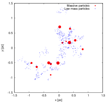
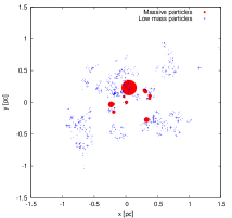
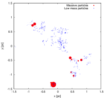
Figure 2: Examples of the three different initial distributions of massive stars assumed in this work (shown in 2D). Red filled circles are high-mass stars ($M\geq 4$ M_⊙) and blue points are low-mass stars ($M<4$ M_⊙). The sizes of circles and points are proportional to the mass of the stars. Left panel: initial fractal with random placement of the masses (NO-SEG). Central panel: initial fractal with inside-out segregation (SEG-IN), i.e. the highest mass stars are in the centre of the distribution. Right panel: initial fractal with outside-in segregation (SEG-OUT), i.e. the highest mass are furthest away from the centre.

In our simulations, we investigate the influence of the initial virial ratio as well. The virial ratio is defined as:

$$Q = \frac{T}{|\Omega|},$$ (2)

i.e. the ratio between kinetic ($T$) and potential ($\Omega$) energy. We start our simulations with values of $Q_{\rm init}=0.2$ and $Q_{\rm init}=0.5$. The values we achieve by re-scaling the kinetic energy, changing the velocities of all stars in a proportional manner.

A value of $Q=0.5$ usually signifies that the system is in virial equilibrium, i.e. it is stable and should not be subject to changes. This is only true for well populated spherical systems and not for the sub-structured distributions, we are using.

Our stellar distributions try to re-arrange themselves into a smaller in size but close to spherical distribution. This produces an initial compression, reaching higher values of $Q$ and then oscillating around the virial state until a stable spherical shape is produced. Starting with a value of $Q_{\rm init}=0.2$ will produce a strong compression, reaching even higher values of $Q$ than in the previous case and then oscillating around the virial state as well, erasing the fractal distribution even faster. An example of this process is shown in Fig. 1. The green dashed line shows the evolution of a fractal with $Q_{\rm init}=0.5$ and the blue solid line for the same fractal now starting with $Q_{\rm init}=0.2$.

We use three different sets of initial distributions for the massive stars. As a massive star we define all stars with $M\geq 4$ M_⊙. Stars less massive are regarded as low-mass stars in our investigation.

The different distribution can be described as follows:

• In the first set we place the masses randomly throughout the fractal distributions, and we refer to this configuration as not segregated: NO-SEG.

• In the second set we force all massive stars to be located within $0.5$ pc and we call it initially mass segregated: SEG-IN.

• In the third set, we locate all massive stars at radii larger than $1.0$ pc to mimic inverse mass-segregation: SEG-OUT.

The SEG-OUT case is very unlikely but we analyze it to test the accepted trend of MS occurring no matter the initial conditions. In Fig. 2 we show the projected distribution of one representative fractal for each initial massive star distribution. Red filled circles are high-mass stars and blue points are low-mass stars. The different sizes of circles and points are proportional to the mass of the stars. The left panel shows an initial fractal with NO-SEG placements of the masses. The central panel is an initial fractal with SEG-IN configuration. The right panel shows the initial fractal with SEG-OUT placement. The number of high-mass stars is ruled by the random sampling of the IMF, but we ensure that in each random realization at least eight massive stars are present.

2.2 Mimicking the gas distribution

To explore the impact of the distribution of gas, we mimic the remaining gas by using two different analytic background (BG) potentials.

For the first set of simulations we use a Plummer potential (Plummer, 1911):

$$\rho(r) = \frac{3{M}_{\rm Pl}}{4\pi R_{\rm Pl}^{3}}\left(1+\frac{r^{2}}{R^{2}_{\rm Pl}}\right)^{-\frac{5}{2}}$$

$$M(r) = M_{\rm Pl}\frac{r^{3}}{R^{3}_{\rm Pl}}\left(1+\frac{r^{2}}{R^{2}_{\rm Pl}}\right)^{-\frac{3}{2}}$$ (3)

$$\Phi(r) = -\frac{GM_{\rm Pl}}{R_{\rm Pl}}\left(1+\frac{r^{2}}{R^{2}_{\rm Pl}}\right)^{-\frac{1}{2}}$$

with ${M}_{\rm Pl}$ and $R_{\rm Pl}$ the Plummer Mass and Plummer radius respectively.

The second set of simulations follows a uniform density profile of the form:

$$\rho(r) = \frac{3M_{\rm tot}}{4\pi r^{3}_{\rm c}}$$

$$M(r) = M_{\rm tot}\frac{r^{3}}{r^{3}_{\rm c}}$$ (4)

$$\Phi(r) = \frac{GM_{\rm tot}}{2r^{3}_{\rm c}}\left(r^{2}-3r_{\rm c}^{2}\right)$$

with ${M}_{\rm tot}$ the total mass of the sphere. The radius of the uniform sphere is given by $r_{c}$.

We choose $M_{\rm Pl}=3472$ M_⊙ and $R_{\rm Pl}=1.0$ pc. For uniform case we have $M_{\rm tot}=3455$ M_⊙ and $r_{\rm c}=1.8$ pc. Both distributions ensure that we have exactly a gas-mass of $M_{\rm gas}(1.5{\rm pc})=2000$ M_⊙ within the stellar distribution, which extends out to a radius of $1.5$ pc. As we have $\sim 500$ M_⊙ in stars, this ensures a star formation efficiency (SFE) of $\epsilon=0.2$.

2.3 The $\Lambda_{\rm MSR}$ parameter

There are many methods to measure MS in a cluster, for example the minimum spanning tree method $\Lambda_{\rm MSR}$ (Allison et al., 2009), the $\sum_{\rm LDR}$ method (Maschberger & Clarke, 2011) and a technique where every distance of the most massive stars to the centre of each group is measured (Kirk & Myers, 2011; Kirk et al., 2014).

Some methods were tested by Parker & Goodwin (2015) resulting, in many cases, in contradictory results as they define MS differently. The authors concluded that the $\Lambda_{\rm MSR}$ method is able to measure MS not only in the classical cases but it is also very efficient and produces reliable results for sub-structured regions.

Based on this study we use the $\Lambda_{\rm MSR}$ method in our investigation. One advantage in using this method, especially for clusters with substructures, is that it is not necessary to define a centre, where the density is highest. In a sub-structured distribution, one might not have a clear high density centre or even worse two or more over-densities within the cluster. Another advantage is that this method includes an associated error, giving information of how reliable the measurement of the MS is.

This method measures the length of the minimum spanning tree (MST; shortest connection between all stars of the sample without crossings) of the $N$ most massive stars $l_{\rm massive}$ and compares it with the MST of the same number of low-mass stars. As we have many combination possibilities as there are many more low-mass stars present, we choose in total $1600$ different random samples of low-mass stars and calculate a mean length of their MSTs $\langle l_{\rm norm}\rangle$ as well as the respective standard deviation $\sigma_{\rm norm}$:

$$\Lambda_{\rm MSR} = \frac{\langle l_{\rm norm}\rangle}{l_{\rm massive}}\pm\frac{\sigma_{\rm norm}}{l_{\rm massive}}$$ (5)

where $\Lambda_{\rm MSR}$ is the degree of MS. $\Lambda_{\rm MSR}\sim 1$ indicates no MS, $\Lambda_{\rm MSR}>>1$ indicates strong MS and $\Lambda_{\rm MSR}<1$ means inverse MS.

In our study we use $N=8$, as this is the minimum number of high mass stars in our samples of the IMF.

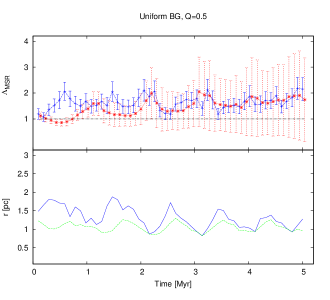
Figure 3: Example of one fractal with an initial mass distribution SEG-OUT, $Q_{\rm init}=0.5$ and an uniform BG. Top panel shows the evolution of $\Lambda_{\rm MSR}$ as red dashed line and stars. The evolution of the $\Lambda_{\rm rest}$ method is denoted with the blue solid line and plus signs. For clarity the $\Lambda_{\rm MSR}$ symbols are slightly shifted in time. The bottom panel compares the evolution of $r_{8}$ (blue solid line) and the value of $R_{h}$ (green dashed line).

2.4 Restricted minimum spanning tree method ($\Lambda_{\rm rest}$)

The measurements of $\Lambda_{\rm MSR}$ can be very sensitive to low mass stars getting kicked out due to strong two-body interactions increasing the values of $l_{\rm norm}$. This can be fixed to some degree, repeating the measurements for $l_{\rm norm}$ many times (in our case $1600$; see above).

A different source of error, can be the escape of one massive star from the cluster, increasing the length of $l_{\rm massive}$ significantly. A similar effect has a massive star, e.g. in the SEG-OUT configuration, on a rather circular orbit around the cluster, i.e. not taking part in any interactions and therefore not subject to any process driving it towards the centre.

Trying to avoid these problems, we restrict the measurements of $\Lambda_{\rm MSR}$ by three conditions:

1. For the determination of $l_{\rm massive}$ we use all massive stars inside of the half-mass radius ($R_{\rm h}$).

2. If it is not possible to find at least eight of the massive stars inside of $R_{\rm h}$, we increase the search radius until we find the eighth massive star $r_{8}$ and base the determination of MS on this radius.

3. For the determination of $l_{\rm norm}$ we only use low-mass stars inside of $2r_{8}$, which can be equal to $2R_{\rm h}$, when at least eight of the massive stars are inside of $R_{\rm h}$.

This restricted method we call $\Lambda_{\rm rest}$. We compare the values obtained from this restricted method with the unrestricted ones (see Sect. 2.3) in all our simulations.

In Fig. 3, we show the evolution for a fractal with initial mass distribution SEG-OUT as an example. In the top panel we show the evolution of $\Lambda_{\rm MSR}$ in red stars connected by a dashed line and $\Lambda_{\rm rest}$ as blue plus-signs connected by a solid line. In the bottom panel we show the evolution of $R_{\rm h}$ (green dashed line) and $r_{8}$ (blue solid line) for the same simulation.

First, we note that towards the end of the simulation both methods give within the errors the same final result which is somewhat reassuring. At the start of the simulation we see significant differences between the two methods. The unrestricted method shows a very low value of MS, as expected for an inside-out simulation, reaching a value of two (a significant value for MS) after more than $2$ Myr and leveling out at a final value of about two. In contrary the restricted method shows a level of MS which is increasing immediately, reaching a value above two in about half a Myr. Furthermore, the unrestricted method shows much larger error-bars.

How can we understand this behaviour? This simulation has more than 8 massive stars ($12$). If some stars are not taking part in MS (as explained above) or get ejected, the range of values for $\Lambda_{\rm MSR}$ can be large leading to a large dispersion of the results reflected in the error-bars. It also gives us the expected low values to begin with, as we are starting with the high-mass stars in the outskirts of the cluster. The restricted method focuses on the innermost $N=8$ stars and shows that they are moving almost immediately to the centre. Both methods show strong oscillations of the $\Lambda$ values, leveling off after about $3$ Myr, showing within the errors slightly higher values for the restricted method than for the unrestricted.

What is the ’true’ value of MS? We would argue, there is no ’correct’ value for the MS, as it depends on your point of view. If you focus on the inner parts of the newly formed cluster only, you will detect a sufficient level of MS almost immediately after just half a Myr (as shown with the restricted results). But, if you have the whole region, in which the stars have formed, in sight, then you detect ejected stars and stars orbiting the new cluster at larger distances, giving you a whole range of MS values, depending on the sample of high-mass stars you pick (large error-bars at the end of the simulation for the unrestricted method). This ambiguity is also visible in the difference between $r_{8}$ and $R_{\rm h}$. In the SEG-OUT simulations we see that $r_{8}$ is always larger than $R_{\rm h}$ and only at later stages they start to agree.

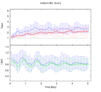
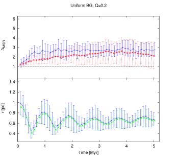
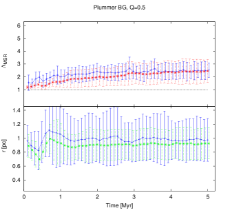
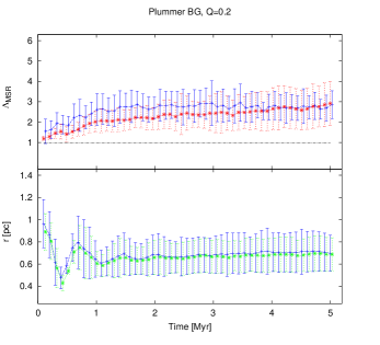
Figure 4: Results for NO-SEG, i.e. the masses are distributed randomly throughout the whole fractal. In contrary to Fig.3 each data-point is a mean value calculated from ten different random realisations. Top row panels show the results for a uniform background and the lower row panels for the Plummer background. Left panels are the simulations with $Q_{\rm init}=0.5$, i.e. starting in ’pseudo-virial equilibrium’ and right panels show the simulations where velocities are reduced to obtain $Q_{\rm init}=0.2$. In each panel the top half shows the evolution of $\Lambda_{\rm MSR}$ (red stars and dashed lines) and $\Lambda_{\rm rest}$ (blue plus signs and solid lines). In the lower halves of the panels we show the evolution of $R_{\rm h}$ (green dashed line) and $r_{8}$ (blue solid line).

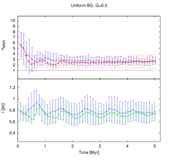
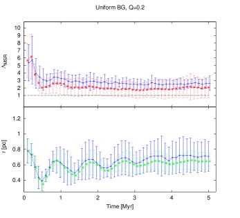
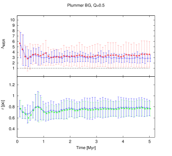
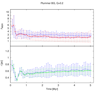
Figure 5: Same as in Fig. 4 but now for the SEG-IN simulations, i.e. where all the massive stars are initially within the central $0.5$ pc.

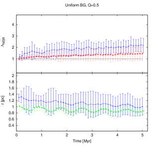
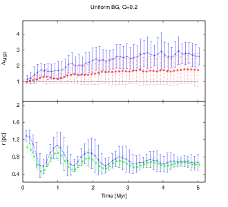
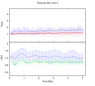
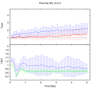
Figure 6: Same as in Fig. 4 but now for the SEG-OUT simulations, i.e. where all the massive stars are initially outside the central $1.0$ pc.

2.5 Set of simulations

We perform, in total, $480$ N-body simulations using the direct N-body integrator code NBODY 6 (Aarseth, 2003) with $1000$ different mass particles with sub-virial, virial and clumpy initials conditions embedded in two different BG potentials.

We use $12$ different fractal distributions for the initial positions. For each fractal we draw a different IMF sample. We use four fractals with their respective IMF samples (position–mass pair) for each set of initial mass placement cases (NO-SEG, SEG-IN and SEG-OUT). For each pair of positions and masses we generate 10 different random assignments of the masses to the positions, following the general rule of each case. This gives us for each case $40$ different sets of initial conditions ($120$ in total), thereby overcoming the influence of by-chance results far from the mean values.

All these sets are now placed into two different background potentials (uniform and Plummer) and are simulated using velocities scaled to a pseudo equilibrium ($Q_{\rm init}=0.5$) or to a cold case with $Q_{\rm init}=0.2$.

3 Results

In the following sub-sections we present the results for the different initial MS states, namely NO-SEG, SEG-IN and SEG-OUT.

The figure shown for each sub-section shows in the left panels the pseudo-virial initial conditions and in the right panels the results for the sub-virial initial state. The top panels are the uniform background simulations, while the lower panels show the results for the background potential which follows a Plummer distribution. The upper half of each panel shows the evolution of the MS ($\Lambda_{\rm MSR}$ and $\Lambda_{\rm rest}$ respectively) and the lower half the evolution of $R_{\rm h}$ and $r_{8}$. In all figures we show the mean values taken from all $40$ realisations of this set of parameters, instead of the results of one single simulation. Again, the unrestricted method is shown as red stars and dashed lines, while the restricted values are given as blue plus-signs and solid lines in the upper part of each panel, while the lower parts show $r_{8}$ in solid blue and $R_{h}$ in dashed green.

3.1 NO-SEG

In Fig. 4, we see in the top parts of each panel, that both methods pick up a $\Lambda$ value (here the term $\Lambda$ refers to both methods) close to one initially. The restricted method shows a slightly larger $\Lambda$ value than the unrestricted one, an efect we have discussed above and we will come back to in the discussion below. The simulations end up with mean values between $2.0$ and $3.0$.

In the top left panel (uniform BG, $Q_{\rm init}=0.5$) we see an increase until about $1.5$ Myr. Afterwards, we see small oscillations around a value of slightly below $3$. At about $4.3$ Myr the highest degree of MS is found ($\Lambda_{\rm rest}=2.98$). As a final value we assign a mean value of $\Lambda_{\rm rest}$ measured from all data-points between $4$ and $5$ Myr called $\Lambda_{\rm final}$, which in this case is $\Lambda_{\rm final}=2.68\pm 0.86$. We call the time where the level of $\Lambda_{\rm rest}$ remains larger than $2$, (i.e. a significant level of MS) $t_{\rm seg}$. In this set of simulations we find $t_{\rm seg}=0.39$ Myr.

In the bottom half of this panel we see small oscillations in $R_{\rm h}$, which are damping out with time and settling at a slightly lower value than the initial one, i.e. we see that even in the supposedly virialised case we get a net contraction of the final cluster.

The top-right box is showing the results for the same background potential but now starting in a cool state ($Q_{\rm init}=0.2$), i.e. undergoing a strong collapse at the beginning. Starting with the same initial degree of MS (as both sets rely on the same initial fractals and mass assignments, just with differently scaled velocities) a stronger increase of $\Lambda_{\rm rest}$ is observed reaching the highest value of $\Lambda_{\rm rest}=3.01$) at already $1.47$ Myr. After that, the variations are smaller than in the ’virial’ case leading to a final mean value of $\Lambda_{\rm final}=2.76\pm 0.82$. Again, both methods agree well within their errors, with the restricted method showing slightly larger values of MS. The value of $t_{\rm seg}=0.39$ Myr.

In the bottom half of this panel we can see the strong decrease of $R_{\rm h}$, due to the cold initial conditions. Afterwards, we obtain large oscillations until the simulations settle into a final value much lower than in the pseudo-virialised case.

The bottom-left panel shows the results for the Plummer BG potential starting in pseudo-equilibrium. We see a slow rise in MS leveling off at a final value of $2.51\pm 0.78$. The highest value of $2.68\pm 0.91$ is reached after $2.84$ Myr. For $t_{\rm seg}$ we obtain $0.78$ Myr. Both methods give indistinguishable values towards the end of the simulation.

, ,

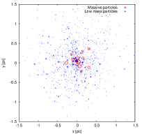
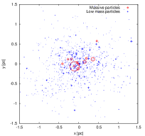
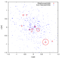
Figure 7: Examples of the final state for the three different initial distribution of massive stars shown in Fig. 2. Left panel: Final state of a fractal which starts with NO-SEG. Central panel: Final state of a fractal which starts with SEG-IN. Right panel: Final state of a fractal which starts with SEG-OUT.

In the bottom half of this panel we see larger error-bars for $R_{\rm h}$. This is explainable by the fact that in a uniform sphere we have a well defined free-fall time which is the same for all radii and so all particles more or less reach the densest configuration at the same time, which is also more or less the same for all simulations of the previous set of parameters. Now, in the Plummer BG case, the free-fall times vary with radius and the point of densest configuration can vary in time for the different sets of initial particle distributions. Therefore, we see no clear oscillations in our results, which are mean values calculated from all simulations, but rather inflated error-bars.

The bottom-right panel shows the results for the Plummer BG potential starting in a cool state i.e. we get a strong compression. We observe a similar trend as in the cold uniform background case: a rise in MS and then an almost constant plateau. The maximum value of $\Lambda_{\rm rest}=3.03$ is reached after $2.16$ Myr. The final value $\Lambda_{\rm final}=2.74$. We measure a $t_{\rm seg}=0.59$ Myr.

In the lower half of this panel, we see that the cold initial conditions produce a similar collapse or contraction in all simulations resulting in small error-bars for $R_{\rm h}$. The steeper potential of the Plummer BG helps to damp the oscillations rather quickly. It settles at about the same value as in the uniform, cold case.

In all four cases we approximately obtain the same values of MS at the end of the simulations. Both methods to measure MS tend to agree within the $1\sigma$ deviations with the restricted method showing slightly higher values. The agreement seems to be better when a Plummer background was used. The simulations with uniform background have shorter values of $t_{\rm seg}$, while we see no difference in this value for the different initial virial states. In all cases a significant level of MS is reached in times shorter than $1$ Myr.

All four panels show an initial contraction or collapse of $R_{\rm h}$. The contraction is stronger in the initially ’cold’ simulations. Oscillations of $R_{\rm h}$ are stronger in the uniform background simulations, while the Plummer background helps to damp the oscillations immediately. This is partly due to the different free-fall times of stars in a Plummer sphere, avoiding a collective oscillation. We see no significant difference in the final values of $R_{\rm h}$ at the end of the simulations for the different background potentials, i.e. we confirm again the findings of Smith et al. (2011, 2013) that this is a function of the initial virial state alone.

3.2 SEG-IN

The sets of simulations (shown in Fig. 5) are designed to have a high value of MS initially, as we have forced the high-mass stars to be in the central area. In all panels we see initial $\Lambda$ values in the range between $5$ and $6$. Also both methods agree at the beginning perfectly as not a single high-mass star is ejected yet. In all simulations we see a rapid decline of the MS values until they settle at roughly the same values as in the NO-SEG cases.

This is in contrary to any prediction of the dynamics of MS in which we should always see an increase. The initial contraction or even collapse (cold simulations) compacts the low-mass stars towards the potential centre. We indentify this initial contraction of the low-mass stars as the main reason for the fastly declining MS values. In all four panels we see an initial decline of $r_{8}$ as well, i.e. also the already centrally concentrated high-mass stars are moving towards the centre as well. This should increase the level of MS; instead we see a rapid decrease in both methods. While in the non-restricted method this could be due to ejected high-mass stars, our restricted method is designed to avoid such results.

The behaviour of $R_{\rm h}$ is similar to the NO-SEG cases explained above.

The top-left panel again shows the uniform BG–$Q_{\rm init}=0.5$ case. The simulations reach a final value of $\Lambda_{\rm final}=2.69\pm 0.69$ with $t_{\rm seg}={\rm always}$ (in fact all panels show $t_{\rm seg}={\rm always}$). The top-right panel shows the results for the uniform BG potential starting in a cool state. Here the final value is $2.56\pm 0.66$. For the Plummer BG with $Q_{\rm init}=0.5$ (bottom left panel) we get $\Lambda_{\rm final}=2.89\pm 0.82$, which is slightly higher than with the uniform BG. It seems that a steeper potential, even though not influencing the final value of $R_{\rm h}$ is able to retain the massive stars in the centre better than the uniform BG. Finally, in the bottom right (Plummer BG–$Q_{\rm init}=0.2$) we get $\Lambda_{\rm final}=2.79\pm 0.68$.

Table 1: Summary of results. The first, second and third column are giving information of the initial conditions: type of BG potential, mass distribution and virial ratio respectively. The fourth and fifth column show the final values for $\Lambda_{\rm MSR}$ and $\Lambda_{\rm rest}$ respectively. The values are calculated by taking an average value of all measurements between 4 and 5 Myr. The sixth column gives $t_{\rm seg}$ i.e. the information when ($t_{\rm seg}$) $\Lambda_{\rm rest}$ stays larger than 2, i.e., a significant level of MS is detected. The last two columns are the final values for $r_{8}$ and $R_{h}$ respectively. Again we calculate them as averages from all measurements between 4 and 5 Myr.

Potential	Mass placement	$Q_{\rm init}$	$\Lambda_{\rm MSR,final}$	$\Lambda_{\rm final}$	$t_{\rm seg}$ [Myr]	$r_{8}$ [pc]	$R_{h}$ [pc]
Uniform	NO-SEG	$0.5$	$2.35\pm 0.94$	$2.68\pm 0.86$	$0.4$	$0.82\pm 0.20$	$0.79\pm 0.14$
Uniform	NO-SEG	$0.2$	$2.32\pm 1.38$	$2.76\pm 0.82$	$0.4$	$0.69\pm 0.19$	$0.65\pm 0.11$
Plummer	NO-SEG	$0.5$	$2.65\pm 1.53$	$2.51\pm 0.78$	$0.8$	$0.90\pm 0.24$	$0.86\pm 0.17$
Plummer	NO-SEG	$0.2$	$2.78\pm 1.13$	$2.74\pm 0.74$	$0.6$	$0.65\pm 0.12$	$0.64\pm 0.10$
Uniform	SEG-IN	$0.5$	$2.58\pm 1.24$	$2.69\pm 0.69$	always	$0.77\pm 0.17$	$0.73\pm 0.13$
Uniform	SEG-IN	$0.2$	$2.03\pm 1.39$	$2.56\pm 0.66$	always	$0.71\pm 0.21$	$0.64\pm 0.11$
Plummer	SEG-IN	$0.5$	$3.49\pm 2.28$	$2.89\pm 0.82$	always	$0.79\pm 0.16$	$0.77\pm 0.14$
Plummer	SEG-IN	$0.2$	$2.20\pm 1.55$	$2.79\pm 0.68$	always	$0.64\pm 0.18$	$0.61\pm 0.12$
Uniform	SEG-OUT	$0.5$	$1.43\pm 0.58$	$2.12\pm 0.57$	3.5	$1.02\pm 0.32$	$0.87\pm 0.14$
Uniform	SEG-OUT	$0.2$	$1.72\pm 0.91$	$2.70\pm 0.72$	1.3	$0.68\pm 0.16$	$0.63\pm 0.07$
Plummer	SEG-OUT	$0.5$	$1.18\pm 0.50$	$1.61\pm 0.39$	never	$1.22\pm 0.31$	$0.97\pm 0.16$
Plummer	SEG-OUT	$0.2$	$1.43\pm 0.69$	$2.14\pm 0.60$	3.8	$0.86\pm 0.38$	$0.69\pm 0.12$

3.3 SEG-OUT

In this section we describe our results (shown in Fig. 6) obtained with rather unusual initial conditions (even though some authors claim to measure inverse mass segregation e.g. in Taurus Parker et al., 2011), i.e. we start with all high-mass stars being formed in the outskirts ($>1$ pc) of the stellar distribution. This is inverse MS and should be reflected by initial $\Lambda$ values below unity. Still, as a mean value taken from $40$ simulations we see a value close to unity, i.e. no segregation. While most simulations in our sample indeed have values below unity, this rather high mean value is due to some special cases in which many high-mass stars are located close to each other but still outside the central area. It is in fact a curiosity produced due to the fractal initial distributions we are using together with the single criterion that high-mass stars have to be outside the central $1$ pc area. We do not force the $\Lambda$ values to be below unity. In one particular simulation we even obtain a value of $\Lambda_{\rm rest}=1.8$.

In the pseudo-equilibrium cases (left panels), we see no fast evolution in MS but a slow increase with the uniform BG ($\Lambda_{\rm final}=2.12\pm 0.57$ and $t_{\rm seg}=3.5$ Myr) or almost no evolution at all with the Plummer BG ($\Lambda_{\rm final}=1.61\pm 0.39$ and $t_{\rm seg}={\rm never}$). This shows that the small contraction of our stellar distribution is not enough to ensure sufficient interactions between the high-mass stars and the lower mass stars to drive them efficiently towards the centre. How realistic such initial conditions are, is debatable.

If we look at the cold cases (right panels), we see again a very fast evolution of MS. Here, it seems the initial collapse of the stellar distribution is enough to drag the high-mass stars to the central area and then they stay there. We get for the uniform BG case a value of $2.70\pm 0.72$ with a $t_{\rm seg}=1.3$ Myr and for the Plummer BG case $2.14\pm 0.60$ and $t_{\rm seg}=3.8$ Myr.

The bottom halves of the panels show again the same evolution of $R_{\rm h}$ as seen in the other sets, but this time we note that the values for $r_{8}$ are always larger than $R_{\rm h}$ for all initial conditions and throughout the simulation times. This means that in all simulations we never got 8 or more massive stars within the half-mass radius.

4 Summary & Discussion

A summary of the most important initial parameters and the associated results is given in Tab. 1.

In Fig. 7 we show the final configurations for the three example simulations shown in Fig. 2. In the left and central panel one clearly sees the effect of MS. In the right panel (SEG-OUT case) the results are debatable, but still an over-density of massive stars can be detected in the centre. In fact this particular example has indeed a final value higher than two.

All sets of simulations (except the SEG-OUT cases) reach values of $\Lambda_{\rm rest}\geq 2$ very fast (less than 1 Myr) or even show these values from the start (SEG-IN).

This shows that it is possible to observe MS after very short times in the embedded phase for clusters which are not initially segregated, so the premise where MS has to be primordial (e.g. Bonnell & Davies, 1998; Hillenbrand & Hartmann, 1998; Raboud & Mermilliod, 1998) is not strictly necessary. Parker et al. (2015) found that primordial MS is less common when in the process of star formation the influence of feed-back is taken into account. However, we cannot exclude primordial MS, which is supported by hydrodynamical simulations (e.g. Klessen, 2001b; Bonnell et al., 2001; Bonnell & Bate, 2006) or even a mix of both effects as shown by Kuznetsova et al. (2015).

After gas-expulsion, the naked SC can inherit the level of MS from the embedded phase, which can be used as an initial condition for studies of later evolution (e.g. McMillan et al., 2007; Moeckel & Bonnell, 2009b; Allison et al., 2009).

The global evolution, in the scenario SEG-OUT, is slower due the location of the massive stars. The low gravitational potential of a Plummer BG in the outer parts joined with a weak compression ($Q_{\rm init}=0.5$) is not producing a significant level of MS. In comparison, the flat uniform BG, which is stronger in the outer parts, is helping to drag most of the massive stars to the centre. For the cool initial state, the Plummer BG is helping the massive stars to reach locations with a deeper potential but not within a short time interval.

Allison et al. (2010), Yu et al. (2011) and Parker et al. (2014) performed similar N-body simulations but without any background potential for the gas distribution. When starting with initially virial (in reality pseudo-virial) conditions they obtain MS values around $\sim 2$. In their cold simulations they obtain MS values of about $6$ (Allison et al., 2010) or even larger than $20$ (Yu et al., 2011). While our MS values in the pseudo-virial case are somewhat higher they mainly agree within the errors. In fact we obtain similar results as the median values of Parker et al. (2014). We believe the reason for the differences can be found in the use of the background potential which is helping to retain stars (in this case high-mass stars) in the central cluster area, which otherwise would have been ejected or at least transported to larger radii. In the initially cold simulations, we see a strong collapse of all stars alike, transporting many low-mass stars to the central areas as well. This lowers our values of MS significantly and by using a background potential, we also keep more low-mass stars from being ejected.

We have to discuss the different values of the $\Lambda_{\rm MSR}$ and $\Lambda_{\rm rest}$ parameters in our simulations. We suggest that the use of $\Lambda_{\rm rest}$ produces more reliable results, even though due to the radius restriction for the low-mass stars, the values are slightly higher than in the unrestricted case. We have tested different radius criterions for the low-mass stars. If we would use the same radius as for the high-mass stars we would always get $\Lambda_{\rm rest}$ values close to unity. Without restriction we would have very similar values than the unrestricted case ($\Lambda_{\rm MSR}$). Therefore our criterion of a restrcition radius of double the length of $r_{8}$ or $R_{\rm h}$ respectively seems to give the most reliable results, without dealing with escapers or high-mass stars orbiting the outskirts of a cluster. This also leads to smaller error bars than in the unrestricted method.

Running our simulations leads to a contraction of the distribution in the pseudo-virialised case or to a collapse in the cold simulations, resulting in a more spherical symmetric and far more denser distribution of the stars. This process is very fast (less than 1 Myr) and very effective in depositing almost all high-mass stars in the central area (NO-SEG and SEG-IN cases; see left and middle panel in Fig. 7). Even in the SEG-OUT case we do see many high-mass stars in the centre. Per definition this should be a highly mass-segregated configuration. But not only the high-mass stars are now centrally concentrated, the low-mass stars are also more centrally concentrated than at the beginning, leading to a high probability for short MSTs, which enter the calculation of $\Lambda_{\rm MSR}$ and even more so for $\Lambda_{\rm rest}$. This will lead to lower values of MS, and explains why in the SEG-IN case we see a sharp initial drop of the $\Lambda$ values, due to all the low-mass stars settling into a more concentrated distribution.

In our models, no stellar evolution was included which is not realistic, but as we reach significant levels of MS in less than one Myr, i.e. a time in which even the most massive stars of our simulations do not evolve, we are confident that this short-fall of our simulations would not alter the final results. The influence of stellar evolution on our results will be subject of a different investigation in the near future.

5 Conclusions

We have presented simulations of the early evolution of initially cool or pseudo-virial, fractal embedded star clusters. The clusters start with three different initial levels of MS namely NO-SEG, SEG-IN and SEG-OUT. We follow the level of MS using the MST method using all the stars ($\Lambda_{\rm MSR}$) and the same method restricted to $R_{h}$ or $r_{8}$ ($\Lambda_{\rm rest}$).

We conclude that in almost all cases (some exceptions with the SEG-OUT conditions), due to the contraction or collapse (pseudo-virial or cold conditions, respectively) we get significant MS within a short time-span of less than 1 Myr. Or, if one refuses to call our initial conditions a star cluster (i.e., if the term star cluster is only applied to a somewhat spherical and centrally concentrated over-density of stars), then our results imply that as soon as the star cluster is formed it is automatically mass-segregated from the start.

On the other hand our results show, that the distribution of stars inside the cluster have lost any information of their initial birth place and so the question if stars are born mass-segregated cannot be answered by looking at a mass-segregated cluster. The only set of simulations which retained at least part of this initial information is the SEG-OUT case, i.e. the most massive stars are born in the outer parts of the star forming region. Here, some massive stars on rather circular orbits in the outskirts of the cluster (star forming region) do not fully take part in the initial contraction phase and therefore do not get deposited into the central area.

To answer the question if the MS is independent of the properties of the gas in embedded young star clusters, we find a similar degree of MS ($\Lambda_{\rm final}$) independent of the conditions of the gas we use.

We conclude that any combination of initial virial ratio, BG potential, and initial mass distribution can lead to almost the same levels of MS with $\Lambda_{\rm final}\approx 2.6\pm^{0.8}_{0.5}$. The only exception is the SEG-OUT scenario together with pseudo-virial velocities, where this parameter shows somewhat lower values.

The dependence on the stochastic initial conditions of the fractal distributions produces in a few cases results far away from the average values reported in this study and we cannot exclude the possibility that these cases can be observed in reality or in theoretical studies, which may be much more sophisticated (and therefore more time consuming) but have to rely on one or a few simulations only.

Acknowledgments: MF acknowledges financial support of FONDECYT grant No. 1130521, Conicyt PII20150171 and BASAL PFB-06/2007. RD is partly funded through a studentship of FONDECYT grant No. 1130521 and BASAL PFB-06/2007.

References

- Aarseth (2003) Aarseth S.J. 2003, Gravitational N-Body Simulations, ISBN 0521432723, Cambridge, UK: Cambridge University Press
- Allison et al. (2009) Allison R.J., Goodwin S.P., Parker R.J., de Grijs R., Portegies Zwart S.F., Kouwenhoven M.B.N. 2009, ApJL, 700, L99
- Allison et al. (2010) Allison R.J., Goodwin S.P., Parker R.J., Portegies Zwart S.F., de Grijs R. 2010, MNRAS, 407, 1098
- Bate et al. (2003) Bate M.R., Bonnell I.A., Bromm V. 2003, MNRAS, 339, 577
- Bate (2009) Bate M.R. 2009, MNRAS, 397, 232
- Bonatto & Bica (2006) Bonatto C., Bica E. 2006, A&A, 455, 931
- Bonnell et al. (1997) Bonnell I.A., Bate M.R., Clarke, C.J., Pringle J.E. 1997, MNRAS, 285, 201
- Bonnell & Davies (1998) Bonnell I.A., Davies M.B. 1998, MNRAS, 295, 691
- Bonnell et al. (2001) Bonnell I.A., Bate M.R., Clarke C.J., Pringle J.E. 2001, MNRAS, 323, 785
- Bonnell et al. (2001) Bonnell I.A., Clarke C.J., Bate M.R., Pringle J.E. 2001, MNRAS, 324, 573
- Bonnell & Bate (2006) Bonnell I.A., Bate M.R. 2006, MNRAS, 370, 488
- Bonnell et al. (2003) Bonnell I.A., Bate M.R., Vine S.G. 2003, MNRAS, 343, 413
- Carpenter & Hodapp (2008) Carpenter J.M., Hodapp K.W. 2008, Handbook of Star Forming Regions, Volume I, 4, 899
- Cartwright & Whitworth (2004) Cartwright A., Whitworth, A.P. 2004, MNRAS, 348, 589
- Chen et al. (2007) Chen L., de Grijs R., Zhao J.L. 2007, AJ, 134, 1368
- Dale et al. (2012) Dale J.E., Ercolano B., Bonnell I.A. 2012, MNRAS, 424, 377
- Elmegreen (2000) Elmegreen B. 2000, Star Formation from the Small to the Large Scale, 445, 265
- Elmegreen & Krakowski (2001) Elmegreen B.G., Krakowski, A. 2001, ApJ, 562, 433
- Er et al. (2013) Er X.-Y., Jiang Z.-B., Fu Y.N. 2013, Research in Astronomy and Astrophysics, 13, 277
- Farias et al. (2015) Farias J.P., Smith R., Fellhauer M., Goodwin S., Candlish G.N., Blaña M., Dominguez R. 2015, MNRAS, 450, 2451
- Girichidis et al. (2012) Girichidis P., Federrath C., Allison R., Banerjee R., Klessen R. (2012) MNRAS, 420, 3264
- Goodwin & Whitworth (2004) Goodwin S.P., Whitworth, A.P. 2004, A&A, 413, 929
- Gutermuth et al. (2005) Gutermuth R.A., Megeath S.T., Pipher J.L., Williams J.P., Allen L.E., Myers P.C., Raines S.N. 2005, ApJ, 632, 397
- Hillenbrand (1997) Hillenbrand L.A. 1997, AJ, 113, 1733
- Hillenbrand & Hartmann (1998) Hillenbrand L.A., Hartmann, L.W. 1998, ApJ, 492, 540
- Kirk & Myers (2011) Kirk H., Myers, P.C. 2011, ApJ, 727, 64
- Kirk et al. (2014) Kirk H., Offner S.S.R., Redmond K.J. 2014, MNRAS, 439, 1765
- Klessen & Burkert (2000) Klessen R.S., Burkert A. 2000, ApJS, 128, 287
- Klessen (2001a) Klessen R. 2001, From Darkness to Light: Origin and Evolution of Young Stellar Clusters, 243, 139
- Klessen (2001b) Klessen R.S. 2001, ApJ, 556, 837
- Klessen & Burkert (2001) Klessen R.S., Burkert, A. 2001, ApJ, 549, 386
- Kroupa (2002) Kroupa P. 2002, Science, 295, 82
- Kuznetsova et al. (2015) Kuznetsova A., Hartmann L., Ballesteros-Paredes J. 2015, ApJ, 815, 27
- Lada et al. (1996) Lada C.J., Alves J., Lada E.A. 1996, AJ, 111, 1964
- Larson (1982) Larson R.B. 1982, MNRAS, 200, 159
- Larson (1995) Larson R.B. 1995, MNRAS, 272, 213
- Leisawitz et al. (1989) Leisawitz D., Bash F.N., Thaddeus P. 1989, ApJS, 70, 731
- Maschberger et al. (2010) Maschberger T., Clarke C.J., Bonnell I.A., Kroupa, P. 2010, MNRAS, 404, 1061
- Maschberger & Clarke (2011) Maschberger T., Clarke C.J. 2011, MNRAS, 416, 541
- McMillan et al. (2007) McMillan S.L.W., Vesperini E., Portegies Zwart S.F. 2007, ApJL, 655, L45
- Moeckel & Bonnell (2009a) Moeckel N., Bonnell I.A. 2009a, MNRAS, 396, 1864
- Moeckel & Bonnell (2009b) Moeckel N., Bonnell I.A. 2009b, MNRAS, 400, 657
- Murray & Lin (1996) Murray S.D., Lin, D.N.C. 1996, ApJ, 467, 728
- Offner et al. (2009) Offner S.S.R., Hansen C.E., Krumholz M.R. 2009, ApJL, 704, L124
- Parker et al. (2011) Parker R.J., Bouvier J., Goodwin S.P., Moraux E., Allison R.J., Guieu S., Güdel M. 2011, MNRAS 412, 2489
- Parker et al. (2014) Parker R.J., Wright N.J., Goodwin S.P., Meyer M.R. 2014, MNRAS, 438, 620
- Parker et al. (2015) Parker R.J., Dale J.E., Ercolano B. 2015, MNRAS, 446, 4278
- Parker & Goodwin (2015) Parker R.J., Goodwin, S.P. 2015, MNRAS, 449, 3381
- Parker et al. (2016) Parker R.J., Goodwin S.P., Wright N.J., Meyer M.R., Quanz S.P. 2016, MNRAS, 459, L119
- Peretto et al. (2006) Peretto N., André P., Belloche A. 2006, A&A, 445, 979
- Peretto et al. (2007) Peretto N., Hennebelle P., André P. 2007, A&A, 464, 983
- Piskunov et al. (2008) Piskunov A.E., Schilbach E., Kharchenko N.V., Röser S., Scholz R.-D. 2008, A&A, 477, 165
- Portegies Zwart et al. (2010) Portegies Zwart S.F., McMillan S.L.W., Gieles M. 2010, ARAA, 48, 431
- Plummer (1911) Plummer, H.C. 1911, MNRAS, 71, 460
- Proszkow & Adams (2009) Proszkow E.-M., Adams F.C. 2009, ApJS, 185, 486
- Raboud & Mermilliod (1998) Raboud, D., & Mermilliod J.-C. 1998, A&A, 333, 897
- Schmeja & Klessen (2006) Schmeja S., Klessen R.S. 2006, A&A, 449, 151
- Schmeja et al. (2008) Schmeja S., Kumar M.S.N., Ferreira B. 2008, MNRAS, 389, 1209
- Smith et al. (2011) Smith R., Slater R., Fellhauer M., Goodwin S., Assmann P. 2011, MNRAS, 416, 383
- Smith et al. (2013) Smith R., Goodwin S., Fellhauer M., Assmann, P. 2013, MNRAS, 428, 1303
- Testi et al. (2000) Testi L., Sargent A.I., Olmi L., Onello J.S. 2000, ApJL, 540, L53
- Williams (2000) Williams J. 2000, in “Massive Star Birth”, 24th meeting of the IAU, Joint Discussion 3, Manchester, England
- Yu et al. (2011) Yu J., de Grijs R., Chen L. 2011, ApJ, 732, 16
- Zinnecker (1982) Zinnecker H. 1982, Annals of the New York Academy of Sciences, 395, 226