The Evolution of Temperature and Bolometric Luminosity in Type-II Supernovae

Abstract

In this work we present a uniform analysis of the temperature evolution and bolometric luminosity of a sample of 29 type-II supernovae (SNe), by fitting a black body model to their multi-band photometry. Our sample includes only SNe with high quality multi-band data and relatively well sampled time coverage. Most of the SNe in our sample were detected less than a week after explosion so their light curves cover the evolution both before and after recombination starts playing a role. We use this sample to study the signature of hydrogen recombination, which is expected to appear once the observed temperature drops to $\approx 7,000$K. Theory predicts that before recombination starts affecting the light curve, both the luminosity and the temperature should drop relatively fast, following a power-law in time. Once the recombination front reaches inner parts of the outflow, it sets the observed temperature to be nearly constant, and slows the decline of the luminosity (or even leads to a re-brightening). We compare our data to analytic studies and find strong evidence for the signature of recombination. We also find that the onset of the optical plateau in a given filter, is effectively the time at which the black body peak reaches the central wavelength of the filter, as it cools, and it does not correspond to the time at which recombination starts affecting the emission.

1 Introduction

Type II supernovae (SNe) are defined by the prominent hydrogen lines in their spectra. They are believed to originate from the collapse of an iron core of massive stars ($\gtrsim$8 $M_{\sun}$) that retain their hydrogen envelope. The most common sub-type, comprising $\sim 70$ percent of all type II SNe, is characterized by a phase of of a roughly constant magnitude in the optical bands, hence their name type II-Plateau (II-P). This plateau phase typically starts 1–2 weeks after the explosion and lasts for $\sim$100 d. Pre-explosion images have revealed that the progenitors of this class are red supergiants, in the mass range of (7–16 $M_{\sun}$) (Smartt 2015; for individual progenitor detections see e.g. Van Dyk et al. 2003a, Van Dyk et al. 2003b, Van Dyk et al. 2012). Type II-Linear (II-L) SNe constitutes another subclass of type II SNe (e.g., Patat et al., 1994; Arcavi et al., 2012; Faran et al., 2014a, b). They are spectroscopically very similar to type II-P events (Faran et al., 2014b, see), but their light curves are declining in all bands. In both types (II-P and II-L) there is typically a sharp drop in the luminosity after $\sim$100 d and the luminosity starts to follow roughly the exponential decay expected from emission powered by the decay of ⁵⁶Ni. The distinction between these two classes is not well defined, and studies have used different definitions for II-L SNe. However, several recent works have shown that there exists a continuum of decline rates between slow declining and fast declining SNe (Anderson et al., 2014; Faran et al., 2014a), which suggests that a separation into two different classes may be artificial. Other type II sub-classes will not be discussed here. In this paper we focus on the light curves of type II-P and type II-L SNe, without making the distinction between the two types, and refer to them in short as type II SNe. Our goal here is to perform a uniform analysis of the bolometric luminosity and temperature evolution of a large sample of type II SNe and to compare our findings to theoretical models, focusing on the transition to the plateau, which takes place during the first two weeks.

There are several dozen type II SNe with detailed multi-wavelength observations. These are typically presented and analyzed individually (e.g., Leonard et al., 2002b; Maguire et al., 2010; Pastorello et al., 2009; Inserra et al., 2011; Takáts et al., 2014, 2015; Fraser et al., 2011; Tomasella et al., 2013; Dall’Ora et al., 2014; Barbarino et al., 2015; Valenti et al., 2015). There are only a few studies that analyze the bolometric properties and temperatures of a sample of type-II SNe. Bersten & Hamuy (2009) extracted bolometric light curves and effective temperature evolution for 33 SNe II-P, using calibrations for bolometric corrections from 3 well observed SNe. Valenti et al. (2016) derived the effective temperature from black body fits to photometric data of 30 type-II SNe, and calculated pseudo-bolometric light curves by integration over the optical bands. Lusk (2016) provides bolometric light curves and temperatures for 5 peculiar type II-P SNe that originated from blue supergiants, by integrating over the observed photometry and correcting for the missing flux in the UV.

The theoretical interpretation of type II light curves is that the emission until the end of the plateau is dominated by the cooling emission, i.e., the leakage of radiation energy that was deposited in the envelope by the shock that unbinds it (Falk & Arnett, 1977). Energy deposited by the decay of ⁵⁶Ni may contribute to this phase (e.g., Falk & Arnett, 1977; Young, 2004; Utrobin, 2007), but this contribution is found to be subdominant (Nakar et al., 2016). The end of the plateau marks the release of all the internal energy deposited by the shock in the envelope. At later times the SN enters its nebular phase and the entire luminosity is driven by the decay of ⁵⁶Ni.

During the early stages of the light curve ($\sim 1-3$ weeks) the leakage of radiation is facilitated mostly by the drop in the optical depth of the outflow due to its expansion (Arnett, 1980). Models predict that during this phase both the temperature and the bolometric luminosity drop roughly as power-laws in time (Nakar & Sari, 2010; Rabinak & Waxman, 2011; Shussman et al., 2016a). Once the observed temperature drop to $\approx 7000$ K, hydrogen recombination becomes important and a recombination front starts moving from the outside towards inner parts of the ejecta. During this phase, recombination, rather then expansion, is the main driver of the drop in the optical depth of the outflow. As a result the observed temperature remains almost constant while the luminosity starts dropping much more slowly or even rises.

In this work we derive the temperatures and bolometric evolution of 29 type-II SNe with high quality multi-band light curves, by fitting a black body spectrum to their spectral energy distribution (SEDs). As will be discussed extensively below, these are far from trivial. SNe II are not blackbodies, and at different times several effects lead to systematic offsets from a pure black body in various bands. Nevertheless, guided by the data and theoretical insight, we derive the underlying black body properties. We compare the temporal evolution of the temperature and luminosity to theoretical predictions, paying special attention to signs of the recombination processes in the envelope. In Section 2 we describe the contents of our SN sample and the data, in Section 3 we explain how the black body fits to the data are done. Section A describes the results of the fitting and the possible effect of extinction on the results, and Section 5 presents a comparison of our results to theoretical expectations. We summarize our results in Section. 6.

2 The Sample

We construct from the literature a sample of 29 type-II SNe with good temporal coverage and multi-band photometry. The sample mostly relies on the SNe collected in Pejcha & Prieto (2015), Faran et al. (2014a) and (Faran et al., 2014b). The SNe in the sample were required to have sufficiently early data (starting less than 20 days after the explosion) and a well sampled light curves so the early behavior could be compared to the late behavior and to theoretical models. Some objects did not enter the sample despite having well sampled photometric curves, because their data was not good enough to produce good quality temperature and luminosity curves. Ten of the objects have Swift UV observations, 10 have JHK data, and 7 objects have both JHK and UV. The photometric data were corrected for galactic extinction according to Cardelli et al. (1989), but not for host galactic extinction, since there is no method that can provide an accurate estimate for $E(B-V)_{host}$ (see for example the discussion in Faran et al. 2014a). We note however, that Faran et al. (2014a) found that $E(B-V)_{host}$ is typically small, of order 0.1 for nearby SNe. The explosion day is set as the mid-point between the first detection and the last non-detection of the SN, and the uncertainty is conservatively set as half the difference. Distance measurements were collected from NED and averaged, using only distances based on the Tully-Fisher method, Cepheids, and SNe Ia. All of the objects are at low redshift with z$<$0.03. The SN properties and their references are summarized in Table. 1.

Table 1: SN Sample Details

SN name	Bands	Explosion day (MJD)	$\mu$	zhost	Reference
SN1999em	U,B,V,R,I,J,H,K	51476 $\pm$ 4	29.84 $\pm$ 0.05	0.002	Leonard et al. (2002a)
					Pejcha & Prieto (2015)
SN1999gi	B,V,R,I	51519 $\pm$ 4	30.24 $\pm$ 0.04	0.002	Faran et al. (2014a)
SN2000dc	B,V,R,I	51762 $\pm$ 4	32.93 $\pm$ 0.14	0.010	Faran et al. (2014a)
SN2001cm	B,V,I	52064 $\pm$ 1	33.18 $\pm$ 0.10	0.011	Faran et al. (2014a)
SN2001cy	B,V,R,I	52086 $\pm$ 6	33.01 $\pm$ 0.12	0.015	Faran et al. (2014b)
SN2001do	B,V,R,I	52134 $\pm$ 2	32.35 $\pm$ 0.15	0.010	Faran et al. (2014b)
SN2001fa	B,V,R,I	52198 $\pm$ 3	34.24 $\pm$ 3.42	0.017	Faran et al. (2014b)
SN2001x	B,V,R,I	51963 $\pm$ 5	31.59 $\pm$ 0.11	0.005	Faran et al. (2014a)
SN2002gd	B,V,R,I	52553 $\pm$ 15	32.90 $\pm$ 0.21	0.009	Faran et al. (2014a)
SN2003hf	B,V,R,I	52864 $\pm$ 2	35.51 $\pm$ 3.55	0.031	Faran et al. (2014b)
SN2003hk	B,V,R,I	52860 $\pm$ 2	34.41 $\pm$ 0.20	0.023	Faran et al. (2014b)
SN2003iq	B,V,R,I	52920 $\pm$ 2	32.28 $\pm$ 0.08	0.008	Faran et al. (2014a)
SN2003z	B,V,R,I	52665 $\pm$ 5	31.23 $\pm$ 3.12	0.004	Faran et al. (2014a)
SN2004A	B,V,R,I	53007 $\pm$ 7	31.61 $\pm$ 0.32	0.003	Gurugubelli et al. (2008)
					Maguire et al. (2010)
SN2004du	B,V,R,I	53228 $\pm$ 2	33.94 $\pm$ 0.13	0.017	Faran et al. (2014a)
SN2004et	U,B,V,R,I,J,H,K	53271 $\pm$ 1	28.41 $\pm$ 0.07	0.000	Maguire et al. (2010)
SN2005cs	Swift UVOT,U,B,V,R,I,J,H,K	53549 $\pm$ 0	29.36 $\pm$ 0.01	0.002	Pastorello et al. (2009)
SN2006bp	Swift UVOT,U,B,V,r,i	53834 $\pm$ 1	31.11 $\pm$ 0.05	0.004	Quimby et al. (2007)
SN2007od	Swift UVOT,U,B,V,R,I,J,H,K	54399 $\pm$ 8	32.29 $\pm$ 0.17	0.006	Inserra et al. (2011)
SN2008in	Swift UVOT,U,B,V,R,I,J,H	54822 $\pm$ 10	30.52 $\pm$ 0.09	0.005	Roy & Kumar (2012)
SN2009N	Swift UVOT,B,g,V,R,r,I,i,J,H	54845 $\pm$ 11	31.68 $\pm$ 0.08	0.003	Takáts et al. (2014)
SN2009bw	Swift UV,U,B,V,R,I,J,H,K	54917 $\pm$ 3	30.60 $\pm$ 0.02	0.004	Inserra et al. (2012)
SN2009ib	U,u,B,g,V,R,r,I,i,J,H	55041 $\pm$ 10	31.48 $\pm$ 0.31	0.004	Takáts et al. (2015)
SN2012A	Swift UVOT,U,B,g,V,R,r,I,i,J,H,K	55929 $\pm$ 5	29.72 $\pm$ 0.17	0.003	Tomasella et al. (2013)
SN2012aw	Swift UVOT,U,u,B,g,V,R,r,I,i,J,H,K	56002 $\pm$ 1	29.89 $\pm$ 0.07	0.003	Bose et al. (2013)
					Dall’Ora et al. (2014)
SN2012ec	u,B,g,V,R,i,J,H,K	56143 $\pm$ 10	31.57 $\pm$ 0.45	0.005	Barbarino et al. (2015)
SN2013ab	Swift UVOT,U,B,g,V,R,r,I,i	56340 $\pm$ 1	31.71 $\pm$ 0.66	0.005	Bose et al. (2015a)
SN2013by	Swift UV,u,B,g,V,r,i	56407 $\pm$ 11	30.84 $\pm$ 0.15	0.004	Valenti et al. (2015)
SN2013ej	Swift UV *,U,u,B,g,V,R,r,I,i	56497 $\pm$ 1	29.77 $\pm$ 2.98	0.002	Richmond (2014)
					Valenti et al. (2014)

3 Black Body Fitting

We calculate the temperature and bolometric luminosity of the SNe at each epoch by fitting a black-body to the photometric data, according to $\rm L_{bol}=4\pi\sigma T^{4}R^{2}$. We create a two-dimensional grid of temperatures evenly spaced by 20K, and black body radii (R) in the range of 10¹²–10¹⁶cm with spacing that corresponds to 0.002 mag. We then compute synthetic photometry from the black body distribution for every T and R values in each of the filter bands. Since data in different photometric bands were sometimes taken at different epochs, linear interpolation is used to account for the missing epochs. The interpolation is constrained to a maximum of 10 days from the nearest data point at early or late phases (before day 10 or after day 70), and to 20 days during intermediate phases, where the SN properties evolve more slowly.

A correct estimation of the photometric uncertainties is needed when fitting a black body to the photometry. Due to the relatively small number of data points, the fit is sensitive to errors that are under- or over-estimated. We therefore set a minimum value of 0.05 magnitudes to the error (such that the error is the maximal value between the given photometric error and 0.05 mag), which is a typical value for the scatter in our light curves. We assign the effective wavelength of the filter transmission curve to each band, and fit the data to find the black body temperature and radius by minimizing $\rm\chi^{2}$. The uncertainty on the temperature is found by marginalizing the likelihood over the radius and finding the upper and lower temperature where $\rm\chi^{2}=\chi_{min}^{2}+1$. To find the uncertainty in the luminosity, we calculate L_bol for every T and R, and find the contour in which $\rm\chi^{2}=\chi_{min}^{2}+1$. The maximal and minimal values of L_bol are taken to be the upper and lower errors, respectively.

The SN spectrum is expected to follow a black body shape only in a limited frequency range, where $\rm h\nu\sim kT$. At high frequencies the flux is suppressed by line blanketing, and at much lower frequencies, in the Rayleigh-Jeans (RJ) regime, it is predicted to be brighter than the RJ tail due to the fact that the thermalization depth in this range is frequency dependent (Shussman et al., 2016a). We observe both effects in our data, and fit a black body only to the wavelength regions where it provides a good approximation.

In agreement with the theoretical predictions, we see that at high temperatures JHK observations cannot be well described by a standard black body spectrum, and tend to systematically lie above the RJ tail. This effect was recently modeled analytically by Shussman et al. (2016a) and will be further discussed in section 5.3. In the cases where this discrepancy is observed, we use only UV and optical data, and exclude the JHK bands.

As the temperature drops below $\sim 10,000-12,000$K, line blanketing by iron group elements becomes strong and creates a deficiency in the measured UV flux, compared to a pure black body. The main species responsible for the strong absorption are Fe III and Ti III (Kasen & Woosley, 2009). Line opacity is highly sensitive to the temperature, and even a slight cooling of the photosphere induces a fast recombination of Fe III and Ti III to Fe II and Ti II (Kasen & Woosley, 2009; Eastman et al., 1996). The flux absorption becomes stronger and shifts further to the optical bands as the temperature continues to decrease to $~{}8,000$K. Figure.1 demonstrates the effect of line blanketing on the SED of SN2012aw on day 41. Data taken at wavelengths shorter than  5000$\rm\AA$ were found to be affected by line blanketing and were excluded from the fit (grey points), and only bands with wavelengths longer than 5000$\rm\AA$ were used (red points). The resulting black body at a temperature of 6420K fits the red points very well and is also in very good agreement with a spectrum taken at the same epoch. The observed spectrum also confirms the flux cut-off around the $B$-band. In order to determine the time where the flux in each photometric band is suppressed by line-blanketing, we run the black body fitting procedure on each of the following filter groups: UV-UBVRIJHK, UBVRIJHK, BVRIJHK, VRIJHK and RIJHK, i.e., each time excluding the bluest band. We first determine, as an example, when the flux in the UV bands falls below the black body curve by looking at the fit to the UBVRIJHK regime. As long as the temperature is high enough, the UV flux will appear above the black body fit to UBVRIJHK or right on it. However, as the temperature decreases enough such that line blanketing starts to have an effect on the UV flux, the UV data points will drop below the UBVRIJHK curve. We exclude a certain band from the fit when it is 1-$\sigma$ below the black body curve. This means that until that epoch we can use the UV-UBVRIJHK bands to determine the black body parameters, and from that day on we can only use the UBVRIJHK bands to fit the data. This procedure is repeated with the other bands to determine when the U, B, and V bands are affected by line blanketing and need to be excluded. The transition days coincide with the intersection between the temperature curves calculated with the bluest band, and the one calculated without it. Eventually, we construct the final temperature and luminosity curves using the transitions determined for each of the objects.

At early phases, when the temperature is higher than 10⁴K, the peak of $\rm F_{\lambda}$ occurs at wavelengths shorter than 3000$\rm\AA$ and UV observations are therefore crucial to constrain the fit parameters. JHK observations lie far from the peak of $\rm F_{\lambda}$ even at low temperatures ($\sim$6000 K), and therefore do not play a critical role in constraining the temperature. However, due to the exclusion of many of the bluer bands by line blanketing, it is necessary to have more data points in the red to improve the fit, meaning that JHK data become important at late epochs.

In order to quantify the importance of UV and Infra-Red (IR) photometry, we run a simulation and estimate the expected errors on the temperature in the absence of UV and IR. We produce synthetic photometry from black body distributions at temperatures 5000K–25,000K in 1000K bins, simulating a spread in the data using the typical photometric errors in each band. We then fit the synthetic data to a black body, repeating the process 100 times per temperature bin. The mean value and standard deviation (STD) of the best-fitting temperatures are computed, where we treat the STD as a measure of the typical statistical error. The uncertainties deduced from the simulation are presented as a function of the temperature in Figure. 2. From the upper panel of Figure. 2 one can see that at temperatures of $\sim$20,000K, the uncertainties on the temperature are quite high (over 800K) even with UV data. This reflects the fact that $\rm F_{\lambda}$ peaks at $\sim$1300$\rm\AA$, while the effective wavelength of the bluest filter we use ($Swift-uvw2$) is only at 2230$\rm\AA$. Below T=15,000K, fits that do not include UV (but do include U) are able to reproduce the temperature with an accuracy of $\sim$500K. When $U$-band data is excluded, the fit reaches that accuracy below T=12,000K.

At lower temperatures, corresponding to late epochs, most of the flux at wavelengths shorter than the B band is already affected by line blanketing and only bands with effective wavelengths longer than the V band can be used. In the bottom panel of Figure 2 it is evident that JHK data are important at T$>$7000K if the B band is not included, as the STD of the fit temperature is relatively high and rises rapidly with the model temperature. Although fitting with the V, R and I bands is still able to produce errors below 10%, we will see in Section 4.1 that the flux in the V band is typically absorbed by iron blanketing at $\sim$6000K. In the absence of JHK observations, we are left with only 3 data points for many objects - V, R and I. In these cases, it is impossible to determine when the V band falls below the black body curve, since we cannot examine the fit done without V, having only 2 data points at longer wavelengths. As a result, when an object does not have JHK data we typically cannot trust the temperature curve below $\sim$6000K and we do not fit the data below this temperature.

Throughout this paper, we consider only objects with U or UV data to deduce physical parameters at high temperatures (above $\sim$10,000K), and objects with JHK data at low temperatures (below $\sim$6000K).

Figure 1: Black body fit of SN2012aw on day 41. The grey points represent bands that are affected by iron-blanketing and were therefore excluded from the fit. The black body curve fits the data very well above 5000$\rm\AA$, whereas at shorter wavelengths the SED is no longer represented by a black body. A spectrum taken on day 41 (Bose et al., 2013) is also shown to coincide well with the data, and confirms the flux cutoff around the $B$-band.

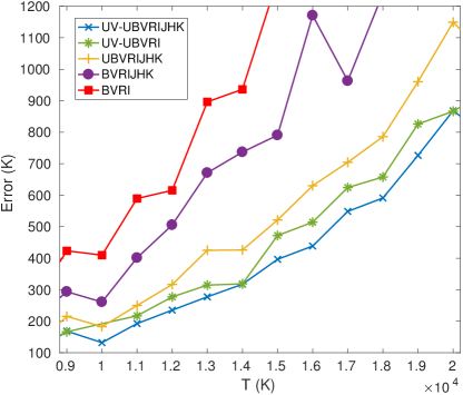
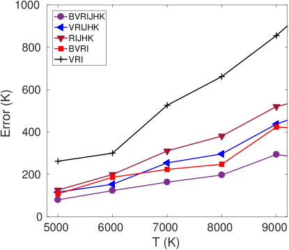
Figure 2: The expected uncertainties of the temperature of a black body, resulting from a simulation of synthetic data. The estimated uncertainties decrease as a function of the proximity of the bands to the black body peak, and therefore rise with the temperature.

4 Results

4.1 Temperature

The temperature curves are computed from the black body fits at each epoch and are presented in Figure. 3 (a list of all the results is also available in Appendix. A). After the explosion, the envelope expands and cools adiabatically. The typical temperatures during the first 10 days are above 10,000 degrees. In cases where UV data exist, the typical errors for that temperature range are smaller than $\sim$500K, and are comparable to the errors predicted by our simulations (see Section 3). Between 20 and 40 days after the explosion, the temperature curves start evolving more slowly compared to early phases. The flattening typically happens between 6000K and 7000K, and is therefore consistent with being associated with a recombination wave that propagates into the envelope and dictates the black body temperature to be the temperature of hydrogen recombination. This effect is analyzed and discussed in Section 5.2. We note that objects without JHK data do not show this flattening, since as discussed in Section 3, for these SNe we were not able to determine the time where the $V$-band can no longer be used and the fit stops when the temperature reaches 6000K.

As in Valenti et al. (2016), we observe that excluding UV data from the fit systematically leads to lower temperatures. This is true also for U, B and V, where the temperature produced without the bluest band is lower than that produced with it, before its flux is affected by iron blanketing. Since we do not observe this behavior in the simulation described in Section 3, the effect is not statistical and points to a deviation of the spectrum from a black body. We suggest that this is related to the re-distribution of energy that is absorbed by line blanketing. Most of the absorbed radiation is expected to be re-emitted close to the absorption wavelength (see Pinto & Eastman, 2000). As a result, the flux of the bluest band we use will be higher than the black body at the same temperature. Since the bands near the peak of the spectrum have the highest effect on the fit, that will result in higher fit temperatures. We redo the fits without the bluest band, and measure the flux under the resulting black body curve. We then measure the flux excess in the bands that lie above the black body curve, and the flux deficiency (due to line blanketing) in the bands below the black body curve and find that they are of the same order. This reinforces the assumption that the absorbed radiation by iron group elements is emitted at wavelengths close to the black body peak, and may add an uncertainty to the temperature and bolometric luminsoity that we measure. Above 10,000K, the temperatures calculated with the bluest band are $\approx 10\%$ higher than the ones calculated when it is omitted, and the difference becomes less significant at lower temperatures. The effect on the luminosity is higher and can get up to $\approx 10-20\%$. Therefore, the temperatures and bolometric luminosities presented in this paper can be overestimated by up to $\approx 10-20\%$.

We record the temperatures at which the flux in different bands starts being affected by line blanketing, and find that the typical temperature for UV is $\sim$11,000K, and $\sim$8000K in the $U$ and $B$ bands. The $V$ band seems to be affected around $\sim$6000K. These results agree with the temperatures shown in Eastman et al. (1996)’s Figure. 7.

Bersten & Hamuy (2009) fit a black body to the photometry of SN1999em corrected to $\rm A_{V}^{host}=0.18$ and present its temperature and bolometric luminosity curves. After correcting our data to $\rm A_{V}^{host}=0.18$, we extract the temperature curve and compare it to the middle panel in Bersten & Hamuy (2009)’s Figure. 8. We find a good agreement between the values of the temperature and its evolution. The temperature computed at the first epoch, $\sim 5$ days, is around 13,000K in both curves and decreases to show a "bump" around day 16. Eventually, both curves settle on a temperature of $\rm\sim 6000K$ in the middle of the plateau. Valenti et al. (2016) also fit a black body to several SNe that are included in our sample, but unfortunately the values are not provided, and we cannot perform a quantitative comparison.

4.2 Luminosity

The bolometric luminosity for each of the SNe is computed from the fit and the curves are presented in Figure. 4. Similarly to the temperature, the luminosity typically decreases as a power law during early epochs. The luminosity in most of the objects relents from its fast decline and starts to decrease more moderately, where the flattening seems to coincide with the break in the temperature. There are 3 objects whose luminosity not only flattens but also starts to rise. This happens for SN2004A and SN2009N at day 30 after explosion, and for SN2005cs at day 23. The transition in luminosity happens quite sharply and occurs when the temperatures are 6000K, 5900K and 6900K for the 3 objects, respectively. The change in the evolution of the luminosity is probably also related to the recombination of the envelope. We will discuss this further in Section 5. At the end of the plateau, the bolometric luminosity falls sharply.

We compare our bolometric luminosity curves to pseudo-bolometric curves from the literature by correcting for the different assumed distances to the SNe, and shifting in time to match the assumed explosion day. While broadly speaking there is mostly agreement between our work and previous efforts, there are still some discrepancies. The comparison is presented in Figure. 5. Pseudo-bolometric luminosities that were not computed with UV nor JHK data, as done for SN2009bw, SN2008in, and SN2004A, can be underestimated by up to 30$\%$.

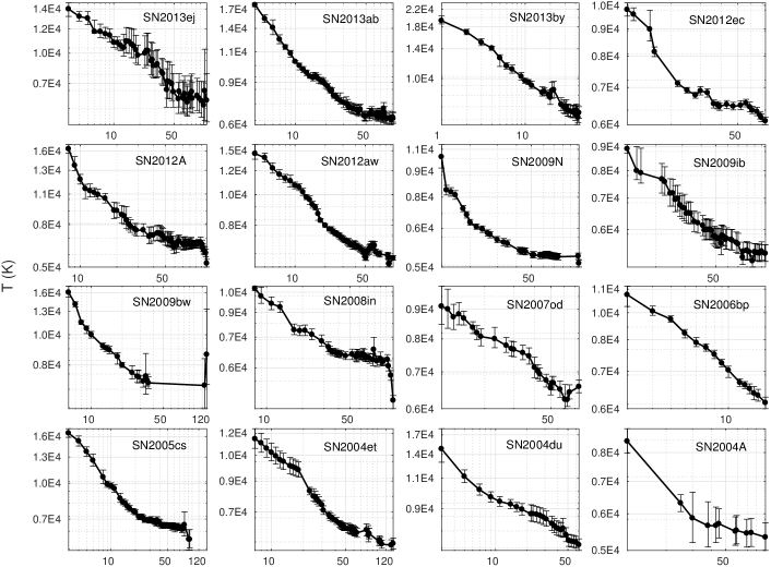
Figure 3: The temperature as a function of time for each SN in the sample.

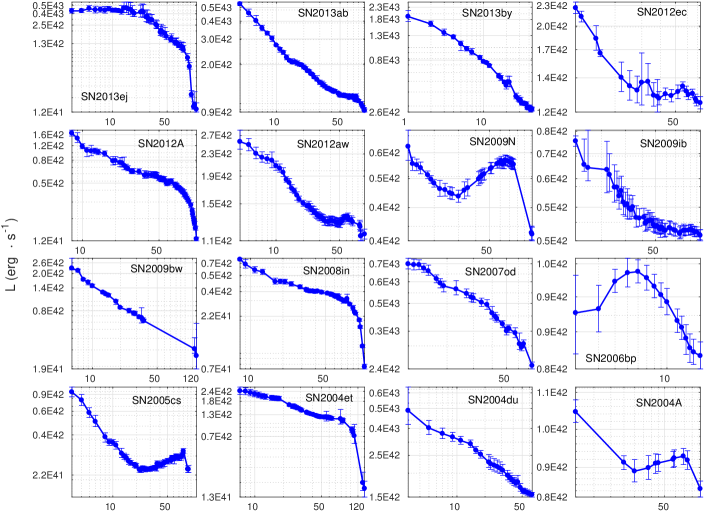
Figure 4: The bolometric luminosity curves as calculated from the black body fits for each SN in the sample.

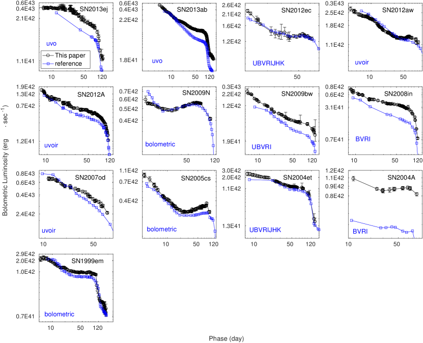
Figure 5: Comparison between the bolometric luminosity curves calculated in this paper (blue) and pseudo-bolometric curves from the literature (red), where the integrated wavelength range is specified. ${}^{\prime}bolometric^{\prime}$ light curves include bolometric corrections or are based on black body fits. Otherwise, the light curves are the integrated luminosity in the observed bands without any bolometric corrections. The luminosity of SN1999em presented here was calculated after correcting for $\rm A_{V}^{host}=0.18$, in order to compare to Bersten & Hamuy (2009). Discrepancies between the curves at early times are probably due to missing UV flux in the pseudo-bolometic curves. SN2012ec (Barbarino et al., 2015), SN2012aw (Dall’Ora et al., 2014), SN2012A (Tomasella et al., 2013), SN2013ab (Bose et al., 2015a), SN2009N (flux in RJ was approximated by RJ tail, no corrections in the blue) (Takáts et al., 2014), SN2009bw (Inserra et al., 2012), SN2008in (Roy & Kumar, 2012), SN2005cs (bolometric corrections) (Pastorello et al., 2009), SN2004et (Maguire et al., 2010), SN2004A (Hendry et al., 2006; Maguire et al., 2010), SN1999em (Bersten & Hamuy, 2009), SN2007od (Inserra et al., 2011), SN2013ej (Bose et al., 2015b)

4.3 The Effect of Extinction

Host interstellar or circumstellar dust can introduce extinction that is not corrected for in our data (see Section 2), resulting in an underestimation of the fit temperatures and luminosities. Although it is quite difficult to find a good estimation for $\rm A_{V}^{host}$, it is possible to quantify the effect a certain Av value has on the fit parameters as a function of the temperature. We repeat the fitting procedure two more times assuming E(B-V) = 0.1 and 0.05, and R_V=3.1, using the galactic extinction laws of Cardelli et al. (1989). As most type-II SNe in or sample are expected to have $\rm E(B-V)^{host}<0.1$ (Faran et al. 2014a), this value is effectively an upper limit on the possible required corrections.

In Figure 6 we present the relation between the best fit temperatures resulting from the correction to $\rm E(B-V)^{host}=0.1$ ($\rm A_{V}^{host}\approx 0.3$) and $\rm E(B-V)^{host}=0.05$ ($\rm A_{V}^{host}\approx 0.1$) as a function of the uncorrected SN temperatures. The dependence of the corrected temperatures on $\rm T(A_{V}^{host}=0$) can be well described by a third order polynomial, according to the following relations:

$$T(A_{V}=0.3)\approx 3.1T_{3}^{3}-58T_{3}^{2}+1630T_{3}-1730$$ (1)

and:

$$T(A_{V}=0.15)\approx 0.69T_{3}^{3}-9.14\times 10^{-2}T_{3}^{2}+1150T_{3}-424,$$ (2)

where $\rm T_{3}\equiv T(Av=0)/10^{3}$. These relations offer a convenient way to estimate the error on a fit temperature, in the typical extinction range of $\rm A_{V}^{host}=0-0.3$ mag.

Since the effect of extinction on the RJ is weak, we expect the luminosity to behave as $\frac{L_{A_{V}}}{L_{0}}=\Big{(}\frac{T_{A_{V}}}{T_{0}}\Big{)}^{3}$ at high temperatures. We fit the data with $\rm T(A_{V}=0)>8000K$ according to this relation for both Av=0.3 and Av=0.15 and present the data and the fit in Figure. 7. This, together with the previous relation for the temperatures, allows also the bolometric luminosity to be corrected for extinction as the relation holds down to low temperatures of $\sim 8000K$. Below that temperature, the corrections to L are less than 10%, which is of the order of the uncertainty.

Figure 6: The best fit temperatures resuting from an extinction correction of $\rm A_{V}^{host}=0.3$ (black dots) and $\rm A_{V}^{host}=0.15$ (blue dots), as a function of $\rm T(A_{V}^{host}=0)$. The grey dashed line indicates $\rm T=T_{A_{V}^{host}=0}$. The third order polynomial fits to the data are plotted in red and can be used to translate between the uncorrected and corrected temperatures.

Figure 7: The ratio between the extinction corrected L_bol ($\rm A_{V}^{host}=0.3$ in black and $\rm A_{V}^{host}=0.15$ in blue) and the uncorrected L_bol, as a function of the similar temperature ratio for $\rm T_{A_{V}^{host}=0}>8000K$. Since extinction has a minimal effect on long wavelength observations, the Rayleigh-Jeans part of the spectrum at high temperatures is expected to be approximately fixed. Therefore, the data follow the relation: $\frac{L_{A_{V}}}{L_{0}}=\Big{(}\frac{T_{A_{V}}}{T_{0}}\Big{)}^{3}$, which is presented by the red line.

5 Comparison to Theory

5.1 The Temperature at the Beginning of the Plateau

The formation process of the plateau in Type-II SNe and the origin of its shape (i.e., its luminosity and temperature evolution) are not fully understood. The common wisdom states that the plateau is formed due to a recombination wave that propagates into the envelope in Lagrangian coordinates. The recombination front defines the photosphere and therefore also fixes its temperature to the temperature of hydrogen recombination in the envelope. According to this view, the plateau should start when T$\approx$7500K. However, more detailed theoretical models show that the peak in each photometric band is observed slightly before the black body peak enters the observed band. This is why redder bands peak at later time. Recombination prevents the observed temperature from falling below $\sim$6000K, which is the main reason that after the peak the luminosity in the optical and IR bands falls rather slowly, and creates what is referred to as the plateau. We therefore expect to find photospheric temperatures higher than 7500K when the plateau starts.

We define the plateau starting time, t_p, in a specific band to be the day at which the light curve changes by less than 0.02 magnitudes per day. To find t_p, we fit a low order polynomial to the first 15-20 days and find the day where the derivative equals 0.02 mag/day. In order to estimate the uncertainties in t_p, we use the photometric errors of the data to generate random Gaussians errors, from which we create simulated data. We run the fit 1000 times on simulated data and use the mean of the results as the value of t_p and the standard deviation as its uncertainty. The value of t_p can be sensitive to the order of the polynomial and to the time range chosen for the fit. The maximal discrepancies introduced by changing those parameters are typically not larger than one day. We therefore set a minimal error of one day on t_p.

In Table 2 we present the t_p values computed in the $R$ and $I$ bands. Some objects have only an upper limit on t_p, since they were first observed already on the plateau. Nevertheless, for most of the objects it is clear that the plateau in $R$ starts slightly before the plateau in $I$, as predicted by theory. In Figure 8 we demonstrate the different locations of the plateau in the $R$ and in the $I$ band for SN2012aw.

The temperatures associated with t_p in $R$ and $I$ are computed by interpolating the temperature curves to t_p. We plot the temperatures at $\rm t_{p}$, i.e. T${}_{\rm p}=T(t=t_{p})$ in the $R$-band for each SN in Figure. 9. The blue arrows indicate the effect that $\rm A_{V}^{host}=0.3$ would have on T_p at $\rm T\approx 8000K$ and $\rm T\approx 11,000K$, according to equation 1. Objects with only lower limits (i.e., first data point lies already on the plateau) are presented by red triangles. Almost all T_p values lie above 8000K, and many of them above 10,000K. The low luminosity SN2005cs shows an exceptionally high lower limit of $T_{\rm p}\gtrsim 16,500$K. The observed range of $T_{p}$ (with the exception of SN2005cs) is consistent with the theoretical light curves prediction by Shussman et al. (2016a). For example, the predicted $R$-band $T_{p}$ for explosion energy of $10^{51}$ erg of progenitors with radii in the range of $400-800~{}R_{\odot}$ and ejecta masses in the range of $7-15~{}M_{\odot}$ is between about 10,000K and 12,000K.

Figure 8: The locations of t_p,R and t_p,I of SN2012aw, as defined by the derivative of the polynomial fit to the $R$-band (blue) and the $I$-band (green). The plateau in the $I$-band appears to start slightly later than the plateau in the $R$-band.

Figure 9: The temperatures at the onset of the plateau phase in the $R$ band. Lower limits are marked by red triangles. The onset of the plateau is defined as the day in which the light curve changes by less than 0.02 magnitudes per day. Most of the temperatures lie above 8000K, which reinforced our claim that the flattening of the light curve is not caused by recombination. The blue arrows show the effect of extinction on T_p at T$\approx$11000K and T$\approx$8000K for A_V=0.3. The plateau temperatures agree with radiative transfer results calculated by Shussman et al. (2016b) for a set of 124 RSGs, represented by the shaded area.

SN name	tp $R$-Band	Tp $R$-band	tp $I$-Band	Tp $I$-band
SN1999em	8.0 (1.0)	11400${}^{+600}_{-800}$	8.0 (1.1)	11400${}^{+700}_{-800}$
SN1999gi	10.0 (1.0)	7900${}^{+400}_{-400}$	10.0 (1.0)	7900${}^{+400}_{-400}$
SN2000dc	13.0 (1.0)	7000${}^{+300}_{-300}$	13.0 (1.0)	7000${}^{+300}_{-300}$
SN2001cm			6.0*	9600${}^{+500}_{-500}$*
SN2001cy	6.0*	11400${}^{+700}_{-700}$*	6.0*	11400${}^{+700}_{-700}$*
SN2001do	8.0 (1.0)	7500${}^{+600}_{-600}$	11.0 (1.0)	7100${}^{+600}_{-500}$
SN2001fa	8.0 (1.0)	10600${}^{+900}_{-1000}$	9.0 (1.0)	10000${}^{+1000}_{-700}$
SN2001x	13.0*	10800${}^{+700}_{-600}$*	13.0*	10800${}^{+700}_{-600}$*
SN2002gd	6.0 (3.0)	10000${}^{+2400}_{-1700}$	6.0 (3.0)	10000${}^{+2400}_{-1700}$
SN2003hf	13.0 (1.0)	10600${}^{+700}_{-700}$	14.0 (1.1)	10400${}^{+700}_{-700}$
SN2003hk	15.0*	10500${}^{+600}_{-600}$*	16.0*	10500${}^{+600}_{-600}$*
SN2003iq	7.0*	9600${}^{+500}_{-500}$*	7.0*	9600${}^{+500}_{-500}$*
SN2003z	9.0 (1.5)	11000${}^{+1100}_{-1100}$	12.0 (1.6)	9300${}^{+700}_{-800}$
SN2004A	11.0*	8000${}^{+400}_{-400}$*	11.0*	8000${}^{+400}_{-400}$*
SN2004du	10.0 (1.0)	9500${}^{+500}_{-500}$	11.0 (1.0)	9300${}^{+500}_{-500}$
SN2004et	9.0*	11600${}^{+800}_{-700}$*	9.0*	11600${}^{+800}_{-700}$*
SN2005cs	3.0*	16400${}^{+800}_{-700}$*	3.0*	16400${}^{+800}_{-700}$*
SN2006bp	8.0 (1.0)	7900${}^{+300}_{-400}$	8.0 (1.0)	7900${}^{+300}_{-400}$
SN2007od	9.0 (1.0)	8700${}^{+600}_{-600}$	9.0 (1.0)	8700${}^{+600}_{-600}$
SN2008in	9.0*	10600${}^{+200}_{-200}$*	9.0*	10600${}^{+200}_{-200}$*
SN2009N	14.0*	10100${}^{+900}_{-800}$*	14.0*	10100${}^{+900}_{-800}$*
SN2009bw	9.0 (1.0)	10900${}^{+900}_{-800}$	11.0 (1.0)	9800${}^{+600}_{-600}$
SN2009ib	13.0*	9100${}^{+200}_{-300}$*	13.0*	9100${}^{+200}_{-300}$*
SN2012A	13.0 (1.7)	10600${}^{+700}_{-400}$	14.0 (1.0)	10400${}^{+600}_{-500}$
SN2012aw	10.0 (1.1)	10800${}^{+300}_{-500}$	13.0 (3.1)	10000${}^{+900}_{-1200}$
SN2012ec	15.0*	10000${}^{+400}_{-400}$*	15.0 *	10000${}^{+400}_{-400}$*
SN2013ab	9.0 (1.0)	11600${}^{+800}_{-900}$	9.0 (1.0)	11600${}^{+800}_{-900}$
SN2013by	8.0 (1.0)	10700${}^{+600}_{-700}$	8.0 (1.0)	10700${}^{+600}_{-700}$
SN2013ej	12.0 (1.6)	10200${}^{+600}_{-600}$	11.0 (1.4)	10400${}^{+600}_{-600}$

Table 2: The times at which the $R$- and the $I$-bands enter the plateau phase, and the corresponding temperatures at those epochs.

5.2 Signs of Recombination in the Temperature and Luminosity Curves

As discussed in Sections 4.1 and 4.2, the evolution of the temperature and the bolometric luminosity is characterized well by a power-law, that flattens when the temperature drops to $\sim$6000–7000K. We compute the early values of the logarithmic derivatives of the luminosity and temperature, $\rm\alpha_{L}$ and $\rm\alpha_{T}$, respectively, during the first 15 days after the explosion. SNe that do not have U or UV data are excluded, since the temperatures at these epochs are typically higher than 12,000K, where U-band data (or bluer) are important to constrain the fit (see Section 3). We also calculate the late logarithmic derivatives between 40 and 100 days, while the SN light curve is on the plateau. For this we choose only SNe with IR data for the reasons discussed in Section 3. The results are summarized in Table 3. The best fit values for the early power law are highly sensitive to the exact value of the zero point in time. Since we make conservative explosion day estimates (see Section. 2), some of the uncertainties on the explosion day are as large as 5-10 days, and introduce non-negligible uncertainties to the values of the power law. The uncertainty values introduced from the fit itself and from the uncertainty on the explosion day are presented separately in Table 3. The values in the parentheses are the errors produced by the fit, and the upper and lower values are the differences from the $\rm\alpha$ values that we get using the lower and upper boundaries of the explosion day estimate, respectively. In cases where the explosion day uncertainty is large (as in SN2013by, SN2012ec, SN2009jb and SN2008in) the upper and lower uncertainties are quite large. However, the explosion day uncertainty naturally has very little effect on the late values of $\rm\alpha$.

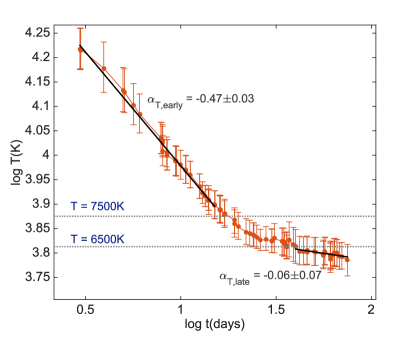
Figure 10: The temperature curve of SN2005cs on logarithmic scale. The temperature behaves as a broken power law, where in early phases it declines rapidly with a power of $\rm-0.47\pm 0.03$, and at late phases the power law is $\rm-0.06\pm 0.07$. This transition in the power law happens within the temperature range 6500–7500K, and we interpret it as the time when the color shell reaches the recombination temperature.

An example of the fit for $\alpha_{T}$ is shown in Figure. 10. It depicts the temperature curve of SN2005cs, on a logarithmic sacale. The best-fit logarithmic derivative computed during the first 15 days is $\rm\alpha_{T}=-0.47\pm 0.03$, and during days 40-100 is $\rm\alpha_{T}=-0.06\pm 0.07$. There is a clear flattening of the temperature curve between t=19d and t=35d, when the temperature is between 6500K and 7500K. In Figure 11 we present the temperature curves and the power law fits for all the objects that have both UV and IR data. From the values of the logarithmic derivatives (table 3) it is clear that at some point the temperature evolution flattens. At early time most values are in the range $\rm\alpha_{T,early}\sim$-0.6 – -0.2 while at late time all best fit values are in the range $\rm\alpha_{T,late}\sim$-0.15 – 0. The weighted mean values of the logarithmic derivatives are $\rm\bar{\alpha}_{T,early}=-0.38\pm 0.01$ and $\rm\bar{\alpha}_{T,late}=-0.08\pm 0.02$. Although it is not possible to point out the exact temperature of the transition, one can see that the range of temperatures between the two power law regimes is $\sim$6000-7000K, which is the temperature range expected from hydrogen recombination in type-II SN envelopes.

We also calculate the early and late logarithmic derivatives of L_bol. Similar to the temperature, the bolometric luminosity curves generally have a higher logarithmic derivative in the early phases. Most of the values of $\alpha_{\rm L,early}$ are between -0.2 and -0.8, while most values of $\alpha_{\rm L,late}$ are between -0.6 and 0.2, with weighted mean values of $\rm\bar{\alpha}_{L,early}=-0.46\pm 0.01$ and $\rm\bar{\alpha}_{L,late}=-0.22\pm 0.03$ . When including the effect of extinction, we find that the values of $\rm\alpha_{T},early$ and $\rm\alpha_{L},early$ increase by $\sim 0.1$ and $\sim 0.2$ respectively, with an extinction value of $\rm E(B-V)=0.1mag$. This result is also consistent with the expectation from recombination which is expected to cause a flatter, or even rising, light curves once the recombination front reaches facilitate the release of radiation from inner regions.

An interesting question is whether there are correlations between the early and late evolution, or between temperature and luminosity evolution. In Figure 12 we plot $\alpha_{\rm T,late}$ vs. $\alpha_{\rm T,early}$ (upper panel) and $\alpha_{\rm L,late}$ vs. $\alpha_{\rm L,early}$ (lower panel). The color coding refers to the decline rate of the $V$-band light curve per 100 days, calculated by linearly fitting the magnitude decline rate between day 25 and 75. The figures show no clear correlations between early and late evolution or between the late decline rate and the temperature evolution (early or late). However, there is a linear correlation between $\rm\alpha_{T}$ and $\rm\alpha_{L}$.

Shussman et al. (2016a) provides theoretical predictions of $\alpha_{\rm T,early}$ and $\alpha_{\rm L,early}$ based on numerical simulations of SN explosions of a large set of RSG progenitors. They find that before recombination $\alpha_{\rm T}$ is not strictly constant, and that it makes a transition from about -0.35 to -0.6. The time of steepening in $\alpha_{\rm T}$ depends on the progenitor radius and ejecta velocity and for typical parameters it ranges between a day and two weeks. Since the data we have is not detailed enough to see the transition between the two power-laws, but only a single average power-law index, the analytic prediction is $\alpha_{\rm T,early}\approx$ -0.35 – -0.6. This range is marked in figure 12 and it is broadly consistent with the observed values listed in table 2. The theoretical model for the luminosity evolution predicts $\alpha_{\rm L,early}\approx-0.35$. This value depends slightly on the progenitor radius (up to about $\pm 0.05$) and more strongly on the progenitor structure (i.e., density profile). comparison of this prediction to the values listed in table 2 shows that they are consistent for most SNe but not for all. Moreover, the value of $\alpha_{\rm L,early}$ is inconsistent with being similar to all SNe. This is probably due to different density profiles of the progenitors.

SN name	$\alpha_{T,early}$	$\alpha_{T,late}$	$\alpha_{L,early}$	$\alpha_{L,late}$
SN1999em	-0.34 (0.06)${}^{+0.18}_{-0.16}$	-0.05 (0.04)${}^{+0.00}_{-0.00}$	-0.54 (0.09)${}^{+0.28}_{-0.25}$	-0.06 (0.06)${}^{+0.01}_{-0.01}$
SN2004et	-0.21 (0.12)${}^{+0.01}_{-0.01}$	-0.11 (0.05)${}^{+0.00}_{-0.00}$	-0.24 (0.17)${}^{+0.01}_{-0.01}$	-0.24 (0.09)${}^{+0.00}_{-0.00}$
SN2005cs	-0.47 (0.03)${}^{+0.00}_{-0.00}$	-0.06 (0.07)${}^{+0.00}_{-0.00}$	-0.68 (0.05)${}^{+0.00}_{-0.00}$	0.13 (0.10)${}^{+0.00}_{-0.00}$
SN2006bp	-0.27 (0.01)${}^{+0.03}_{-0.03}$		-0.04 (0.01)${}^{+0.01}_{-0.01}$
SN2007od	-0.10 (0.27)${}^{+0.06}_{-0.06}$	-0.09 (0.06)${}^{+0.01}_{-0.01}$	-0.22 (0.29)${}^{+0.14}_{-0.14}$	-0.81 (0.09)${}^{+0.12}_{-0.12}$
SN2008in	-0.28 (0.10)${}^{+0.28}_{-0.26}$	-0.07 (0.07)${}^{+0.01}_{-0.01}$	-0.50 (0.12)${}^{+0.49}_{-0.46}$	-0.52 (0.07)${}^{+0.09}_{-0.09}$
SN2009N	-0.48 (0.22)${}^{+0.35}_{-0.34}$	-0.07 (0.05)${}^{+0.01}_{-0.01}$	-0.21 (0.19)${}^{+0.15}_{-0.15}$	0.11 (0.05)${}^{+0.02}_{-0.02}$
SN2009bw	-0.67 (0.05)${}^{+0.23}_{-0.21}$	-0.04 (0.19)${}^{+0.00}_{-0.00}$	-0.79 (0.07)${}^{+0.25}_{-0.24}$	-0.29 (0.10)${}^{+0.01}_{-0.01}$
SN2009ib	-0.29 (0.12)${}^{+0.16}_{-0.15}$	-0.14 (0.08)${}^{+0.02}_{-0.02}$	-0.32 (0.15)${}^{+0.18}_{-0.17}$	-0.03 (0.05)${}^{+0.00}_{-0.00}$
SN2012A	-0.84 (0.11)${}^{+0.38}_{-0.37}$	-0.09 (0.06)${}^{+0.01}_{-0.01}$	-1.07 (0.18)${}^{+0.48}_{-0.47}$	-0.87 (0.07)${}^{+0.06}_{-0.06}$
SN2012aw	-0.35 (0.02)${}^{+0.02}_{-0.02}$	-0.11 (0.04)${}^{+0.00}_{-0.00}$	-0.33 (0.03)${}^{+0.02}_{-0.02}$	-0.09 (0.06)${}^{+0.00}_{-0.00}$
SN2012ec	-0.50 (0.21)${}^{+0.39}_{-0.38}$	-0.11 (0.07)${}^{+0.02}_{-0.02}$	-0.75 (0.22)${}^{+0.58}_{-0.56}$	-0.06 (0.13)${}^{+0.01}_{-0.01}$
SN2013ab	-0.56 (0.02)${}^{+0.07}_{-0.07}$		-0.80 (0.03)${}^{+0.10}_{-0.10}$
SN2013by	-0.30 (0.01)${}^{+0.38}_{-0.84}$		-0.42 (0.01)${}^{+0.49}_{-1.03}$
SN2013ej	-0.21 (0.03)${}^{+0.04}_{-0.03}$		-0.00 (0.05)${}^{+0.00}_{-0.00}$

Table 3: The early and late logarithmic derivatives of the temperature and the bolometric luminosity. The values of $\rm\alpha_{T,early}$ and $\rm\alpha_{L,early}$ increase by $\approx 0.1$ and $\approx 0.2$ respectively, with an extinction value of $\rm E(B-V)=0.1$ mag.

Figure 11: Temperature curves of objects that have both UV and JHK data. The numbers indicate the values of the best-fit early and late logarithmic derivative computed during the first 15 days, and during days 40-100 after the explosion, respectively. A clear flattening of the temperature is observed as the SN approcahes the temperaure of hydrogen recombination.

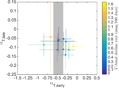
Figure 12: Top: the logarithmic derivative of the temperature at late times (40-100 days after the explosion) vs. the logarithmic derivative of the temperature at early times (up to 15 days after the explosion). The colors represent the decline rate of the $V$-band light curve. The values of the different objects agree with each other within the error-bars, and there is no apparent correlation with the light curve decline rate. Bottom: the same as the top figure for the bolometric luminosity. In this case, the early values of the logarithmic derivatives agree within the errors, but the late values show a wider spread. SNe whose luminosity declines faster at late phases (i.e., during the plateau phase) have faster declining light curves.

5.3 Deviation from Black Body

At high temperatures, we find that a black body is not able to describe the whole observed spectrum not only at short wavelengths, where line blanketing is important, but also at long wavelengths on the RJ tail. In the left panel of Figure. 13 we show the SED of SN2012A on day 8, where the temperature is $\sim$15,000K. The dashed blue line is the best fit to all of the data points, which clearly fails to fit the JHK observations. This effect is observed in all SNe that have early JHK data, which always seem to be brighter than the RJ tail at the temperature corresponding to the optical and UV flux.

Deviation of the RJ tail from a black body spectrum of early type II emission was seen in numerical simulations (e.g., Tominaga et al., 2011) and was modeled recently analytically by Shussman et al. (2016a). According to the model the reason for the deviation is that the flux at different wavelengths is determined at different locations in the outflow at different gas temperatures. Shussman et al. (2016a) find that on the RJ tail the modified spectrum can be approximated as $F_{\nu}\propto\nu^{1.4}$ and they also provide an approximation for the entire spectrum. The black solid line in the left panel of Figure. 13 is the best fit of Shussman et al. (2016a) model to the data of SN2012A. The model seems to fit the data very well throughout the UV and the IR and follows the JHK flux where it departs from a standard black body.

At lower temperatures both the standard black body model and the modified black body models are able to describe the JHK observations, as seen in the right panel of Figure. 13. The reason is that these bands are closer to the peak of the spectrum, where the models are essentially equivalent. Also, at lower temperatures, where recombination starts affecting the spectrum the analytic model is no longer applicable.

Figure 13: left:The SED of SN2012A at 8 days after the explosion. The standard Planck formula is only able to fit the peak of the distribution, but fails to fit the RJ tail. A modified black body model from Shussman et al. (2016a) is shown to be compatible throughout the whole wavelength range. right: An SED of SN2012A at 50 days past explosion. At this stage, after the onset of recombination and at low temperatures, both the modified black body and the standard model are able to describe the data.

6 Summary

We calculated the temperaures and bolometric luminosities of 29 type-II SNe, by fitting black body models to their SEDs. We use the results to study the properties at the beginning of the plateau, to look for the signature of hydrogen recombination and to compare the observation before recombination becomes important to theoretical models. Our main findings are listed below.

• The temperature at the onset of the plateau phase in the $R$-band is above 8000K for all SNe in our sample, and exceeds 10,000K in many of them. This temperature changes as a function of the observed band, and is determined by the temperature at which the peak of the black body spectrum roughly coincides with the center of the filter transmission curve. This result is consistent with recent theoretical models and is different than the common statment that the plateau phase starts once hydrogen recombinations becomes important. The temperatures we find agree with the predicted values for typical RSG progenitors of type-II SNe (Shussman et al., 2016a).

• We find that the temperature evolves with time as a power law, which flattens at $\rm\sim 6000-8000K$. We observe a similar evolution in the bolometric luminosity, where the logarithmic derivative at early phases is higher than that at late phases. The flattening is most likely a result of the recombination wave that exposes the inner layers. The values of the logarithmic derivatives for T and $\rm L_{bol}$ at early phases agree with predictions from simulations and analytic works (Shussman et al., 2016a; Nakar & Sari, 2010).

• SN spectra deviate from a standard black body, both at low temperatures and short wavelengths due to line blanketing, and also at high temperatures and long wavelengths. We show that the SNe in our sample follow the analytic result from (Shussman et al., 2016a), that the flux on the RJ tail follows $F_{\nu}\propto\nu^{1.4}$.

Appendix A A List of the Temperatures and Bolometric Luminosities

Table 4: A List of the Temperatures and Bolometric Luminosities

MJD	$t-t_{\textrm{explosion}}$	T(K)	L(1042 erg $\cdot s^{-1}$)
SN1999em
51481	5	11670${}^{904}_{761}$	1.43${}^{0.19}_{0.14}$
51482	6	11748${}^{841}_{707}$	1.53${}^{0.17}_{0.15}$
51483	7	11493${}^{652}_{597}$	1.50${}^{0.14}_{0.12}$
51484	8	11075${}^{632}_{532}$	1.42${}^{0.13}_{0.10}$
51485	9	10681${}^{576}_{529}$	1.35${}^{0.11}_{0.09}$
51486	10	10320${}^{506}_{441}$	1.27${}^{0.09}_{0.07}$
51487	11	9944${}^{527}_{432}$	1.19${}^{0.09}_{0.07}$
51488	12	9539${}^{415}_{381}$	1.13${}^{0.06}_{0.05}$
51489	13	9250${}^{379}_{336}$	1.08${}^{0.05}_{0.05}$
51491	15	8481${}^{356}_{236}$	1.00${}^{0.04}_{0.04}$
51492	16	8300${}^{272}_{251}$	0.97${}^{0.06}_{0.06}$
51493	17	8340${}^{253}_{220}$	0.99${}^{0.06}_{0.05}$
51494	18	8340${}^{234}_{237}$	1.00${}^{0.05}_{0.05}$
51495	19	8310${}^{245}_{239}$	0.99${}^{0.05}_{0.05}$
51496	20	8160${}^{231}_{228}$	0.96${}^{0.05}_{0.05}$
51498	22	7899${}^{260}_{255}$	0.90${}^{0.05}_{0.05}$
51501	25	7250${}^{176}_{181}$	0.86${}^{0.04}_{0.04}$
51504	28	7320${}^{174}_{178}$	0.85${}^{0.04}_{0.03}$
51505	29	7040${}^{162}_{161}$	0.83${}^{0.03}_{0.03}$
51507	31	7060${}^{162}_{162}$	0.83${}^{0.03}_{0.03}$
51508	32	7040${}^{165}_{158}$	0.83${}^{0.03}_{0.03}$
51510	34	6950${}^{173}_{166}$	0.81${}^{0.03}_{0.03}$
51513	37	6740${}^{149}_{144}$	0.80${}^{0.03}_{0.03}$
51514	38	6600${}^{138}_{141}$	0.81${}^{0.03}_{0.03}$
51516	40	6440${}^{137}_{131}$	0.82${}^{0.03}_{0.03}$
51518	42	6340${}^{124}_{131}$	0.80${}^{0.03}_{0.03}$
51519	43	6320${}^{130}_{124}$	0.80${}^{0.03}_{0.02}$
51520	44	6360${}^{139}_{120}$	0.80${}^{0.03}_{0.02}$
51522	46	6480${}^{136}_{132}$	0.82${}^{0.03}_{0.03}$
51523	47	6460${}^{135}_{132}$	0.83${}^{0.03}_{0.03}$
51526	50	6300${}^{132}_{121}$	0.82${}^{0.03}_{0.03}$
51527	51	6260${}^{125}_{124}$	0.81${}^{0.03}_{0.03}$
51528	52	6260${}^{138}_{113}$	0.81${}^{0.03}_{0.02}$
51530	54	6220${}^{126}_{119}$	0.81${}^{0.03}_{0.02}$
51538	62	6000${}^{115}_{112}$	0.80${}^{0.02}_{0.02}$
51541	65	6033${}^{224}_{137}$	0.80${}^{0.05}_{0.03}$
51546	70	6150${}^{179}_{168}$	0.83${}^{0.04}_{0.04}$
51547	71	6140${}^{172}_{165}$	0.83${}^{0.04}_{0.04}$
51551	75	6270${}^{187}_{172}$	0.83${}^{0.04}_{0.04}$
51556	80	6120${}^{165}_{161}$	0.81${}^{0.04}_{0.04}$
51557	81	5920${}^{312}_{277}$	0.76${}^{0.08}_{0.07}$

Table 5: continued

A List of the Temperatures and Bolometric Luminosities 51558 82 5891${}^{341}_{324}$ 0.76${}^{0.09}_{0.08}$ 51565 89 6080${}^{166}_{169}$ 0.77${}^{0.04}_{0.04}$ 51570 94 6200${}^{164}_{172}$ 0.76${}^{0.03}_{0.04}$ 51572 96 6200${}^{165}_{171}$ 0.74${}^{0.03}_{0.03}$ 51576 100 6480${}^{188}_{183}$ 0.72${}^{0.04}_{0.03}$ 51578 102 6600${}^{193}_{193}$ 0.71${}^{0.04}_{0.04}$ 51581 105 6780${}^{280}_{266}$ 0.69${}^{0.04}_{0.04}$ 51586 110 5400${}^{538}_{449}$ 0.40${}^{0.08}_{0.06}$ 51592 116 4960${}^{447}_{367}$ 0.29${}^{0.05}_{0.04}$ 51599 123 4960${}^{435}_{376}$ 0.21${}^{0.04}_{0.03}$ 51604 128 5500${}^{292}_{247}$ 0.17${}^{0.02}_{0.01}$ 51606 130 5620${}^{233}_{230}$ 0.16${}^{0.01}_{0.01}$ 51607 131 5620${}^{163}_{144}$ 0.16${}^{0.01}_{0.01}$ 51613 137 5640${}^{154}_{162}$ 0.14${}^{0.01}_{0.01}$ 51614 138 5640${}^{161}_{135}$ 0.14${}^{0.01}_{0.01}$ 51619 143 5760${}^{156}_{142}$ 0.14${}^{0.01}_{0.01}$ 51620 144 5760${}^{139}_{147}$ 0.14${}^{0.01}_{0.01}$ 51624 148 5920${}^{151}_{152}$ 0.15${}^{0.01}_{0.01}$ 51627 151 5900${}^{158}_{144}$ 0.14${}^{0.01}_{0.01}$ 51629 153 5940${}^{150}_{155}$ 0.14${}^{0.01}_{0.01}$ 51634 158 5960${}^{159}_{150}$ 0.13${}^{0.01}_{0.01}$ 51637 161 5880${}^{158}_{165}$ 0.12${}^{0.01}_{0.01}$ 51638 162 5160${}^{597}_{454}$ 0.10${}^{0.02}_{0.01}$ 51639 163 5460${}^{707}_{546}$ 0.11${}^{0.03}_{0.02}$ 51640 164 5300${}^{680}_{516}$ 0.10${}^{0.03}_{0.02}$ 51641 165 5024${}^{1549}_{518}$ 0.09${}^{0.06}_{0.01}$ 51642 166 5640${}^{774}_{602}$ 0.11${}^{0.03}_{0.02}$ 51643 167 5880${}^{671}_{531}$ 0.11${}^{0.03}_{0.02}$ 51644 168 5920${}^{751}_{561}$ 0.12${}^{0.03}_{0.02}$ 51650 174 5580${}^{595}_{472}$ 0.09${}^{0.02}_{0.01}$ 51653 177 5400${}^{534}_{450}$ 0.08${}^{0.02}_{0.01}$ 51655 179 6080${}^{727}_{571}$ 0.10${}^{0.03}_{0.02}$ 51656 180 5560${}^{580}_{475}$ 0.08${}^{0.02}_{0.01}$ SN1999gi 51524 5 8680${}^{752}_{611}$ 0.57${}^{0.07}_{0.05}$ 51525 6 8480${}^{347}_{323}$ 0.59${}^{0.03}_{0.02}$ 51528 9 8100${}^{307}_{298}$ 0.65${}^{0.02}_{0.02}$ 51529 10 7880${}^{291}_{280}$ 0.63${}^{0.02}_{0.02}$ 51530 11 7720${}^{276}_{269}$ 0.63${}^{0.02}_{0.02}$ 51531 12 7560${}^{269}_{253}$ 0.62${}^{0.02}_{0.02}$ 51534 15 7436${}^{700}_{307}$ 0.60${}^{0.06}_{0.02}$ 51540 21 6860${}^{411}_{389}$ 0.59${}^{0.03}_{0.02}$ 51545 26 6760${}^{419}_{360}$ 0.56${}^{0.03}_{0.02}$

Table 6: continued

A List of the Temperatures and Bolometric Luminosities 51550 31 6120${}^{334}_{292}$ 0.52${}^{0.02}_{0.02}$ 51556 37 5920${}^{308}_{274}$ 0.50${}^{0.01}_{0.01}$ 51577 58 5320${}^{243}_{219}$ 0.50${}^{0.01}_{0.01}$ 51582 63 5260${}^{232}_{219}$ 0.49${}^{0.01}_{0.01}$ 51590 71 5080${}^{223}_{197}$ 0.50${}^{0.02}_{0.02}$ 51614 95 5140${}^{218}_{211}$ 0.45${}^{0.02}_{0.01}$ 51619 100 4960${}^{200}_{198}$ 0.45${}^{0.02}_{0.01}$ 51624 105 4880${}^{205}_{181}$ 0.43${}^{0.02}_{0.01}$ 51629 110 4880${}^{200}_{185}$ 0.40${}^{0.01}_{0.01}$ 51634 115 4700${}^{178}_{177}$ 0.36${}^{0.02}_{0.01}$ 51638 119 4580${}^{167}_{169}$ 0.31${}^{0.01}_{0.01}$ 51643 124 4220${}^{145}_{139}$ 0.25${}^{0.01}_{0.01}$ 51648 129 4060${}^{211}_{185}$ 0.17${}^{0.02}_{0.01}$ 51653 134 3760${}^{116}_{110}$ 0.13${}^{0.01}_{0.01}$ 51658 139 3300${}^{155}_{142}$ 0.17${}^{0.03}_{0.02}$ 51664 145 3640${}^{104}_{107}$ 0.11${}^{0.01}_{0.01}$ 51669 150 3620${}^{101}_{108}$ 0.11${}^{0.01}_{0.01}$ SN2000dc 51766 4 8540${}^{353}_{327}$ 1.39${}^{0.06}_{0.06}$ 51767 5 8220${}^{327}_{300}$ 1.46${}^{0.06}_{0.05}$ 51773 11 7100${}^{243}_{215}$ 1.70${}^{0.05}_{0.04}$ 51775 13 7020${}^{231}_{214}$ 1.69${}^{0.05}_{0.04}$ 51777 15 6940${}^{226}_{208}$ 1.63${}^{0.04}_{0.04}$ 51779 17 6800${}^{206}_{210}$ 1.55${}^{0.04}_{0.04}$ 51781 19 6540${}^{196}_{187}$ 1.50${}^{0.03}_{0.04}$ SN2001cm 52069 5 9580${}^{494}_{424}$ 1.63${}^{0.11}_{0.09}$ 52070 6 9840${}^{516}_{455}$ 1.73${}^{0.12}_{0.10}$ 52071 7 9960${}^{531}_{467}$ 1.78${}^{0.13}_{0.10}$ 52072 8 9780${}^{507}_{451}$ 1.73${}^{0.11}_{0.10}$ 52077 13 9280${}^{438}_{413}$ 1.54${}^{0.09}_{0.08}$ 52082 18 8300${}^{370}_{329}$ 1.31${}^{0.06}_{0.05}$ 52087 23 7440${}^{303}_{273}$ 1.13${}^{0.04}_{0.04}$ SN2001cy 52092 6 11400${}^{687}_{605}$ 3.32${}^{0.33}_{0.27}$ 52093 7 11140${}^{638}_{587}$ 3.17${}^{0.29}_{0.24}$ 52094 8 10920${}^{615}_{557}$ 3.05${}^{0.27}_{0.22}$ 52095 9 10720${}^{614}_{516}$ 2.95${}^{0.26}_{0.20}$ 52096 10 10620${}^{759}_{668}$ 2.89${}^{0.34}_{0.27}$ 52097 11 10480${}^{548}_{519}$ 2.81${}^{0.22}_{0.19}$ 52098 12 10200${}^{1115}_{886}$ 2.68${}^{0.39}_{0.26}$ 52099 13 10240${}^{535}_{480}$ 2.66${}^{0.20}_{0.17}$

Table 7: continued

A List of the Temperatures and Bolometric Luminosities 52100 14 9878${}^{1460}_{522}$ 2.48${}^{0.63}_{0.18}$ 52102 16 10020${}^{1028}_{853}$ 2.49${}^{0.42}_{0.30}$ 52104 18 9680${}^{954}_{787}$ 2.30${}^{0.36}_{0.26}$ 52106 20 9460${}^{1017}_{812}$ 2.17${}^{0.37}_{0.25}$ 52112 26 8400${}^{699}_{568}$ 1.65${}^{0.18}_{0.12}$ 52117 31 7740${}^{553}_{495}$ 1.38${}^{0.11}_{0.09}$ 52122 36 7260${}^{500}_{422}$ 1.22${}^{0.08}_{0.06}$ 52132 46 6660${}^{402}_{356}$ 1.06${}^{0.05}_{0.04}$ 52137 51 6540${}^{389}_{336}$ 1.02${}^{0.04}_{0.03}$ 52142 56 6440${}^{379}_{322}$ 0.98${}^{0.04}_{0.03}$ 52147 61 6380${}^{357}_{326}$ 0.94${}^{0.04}_{0.03}$ 52152 66 6220${}^{338}_{309}$ 0.90${}^{0.03}_{0.03}$ 52157 71 6080${}^{327}_{290}$ 0.88${}^{0.03}_{0.03}$ 52162 76 5940${}^{323}_{273}$ 0.87${}^{0.03}_{0.02}$ 52167 81 5980${}^{320}_{276}$ 0.86${}^{0.03}_{0.02}$ 52172 86 6060${}^{318}_{294}$ 0.83${}^{0.03}_{0.02}$ 52177 91 5820${}^{291}_{269}$ 0.77${}^{0.02}_{0.02}$ 52182 96 5600${}^{276}_{242}$ 0.71${}^{0.02}_{0.02}$ SN2001do 52137 3 8780${}^{385}_{339}$ 1.34${}^{0.07}_{0.06}$ 52138 4 8117${}^{1077}_{362}$ 1.29${}^{0.22}_{0.05}$ 52139 5 8300${}^{682}_{551}$ 1.42${}^{0.15}_{0.10}$ 52140 6 7780${}^{574}_{490}$ 1.36${}^{0.11}_{0.08}$ 52141 7 7680${}^{544}_{486}$ 1.36${}^{0.10}_{0.08}$ 52142 8 7500${}^{514}_{462}$ 1.35${}^{0.09}_{0.08}$ 52145 11 7100${}^{452}_{412}$ 1.34${}^{0.08}_{0.06}$ 52148 14 6580${}^{387}_{345}$ 1.28${}^{0.05}_{0.05}$ 52151 17 6720${}^{409}_{359}$ 1.19${}^{0.06}_{0.04}$ 52154 20 6360${}^{370}_{312}$ 1.14${}^{0.04}_{0.04}$ 52157 23 6240${}^{332}_{318}$ 1.07${}^{0.04}_{0.03}$ 52160 26 6200${}^{347}_{298}$ 1.03${}^{0.03}_{0.03}$ 52163 29 5900${}^{303}_{274}$ 0.99${}^{0.03}_{0.03}$ 52166 32 5600${}^{271}_{245}$ 0.93${}^{0.02}_{0.03}$ 52169 35 5640${}^{273}_{251}$ 0.87${}^{0.02}_{0.02}$ 52172 38 5520${}^{258}_{241}$ 0.81${}^{0.02}_{0.02}$ 52175 41 5340${}^{239}_{227}$ 0.77${}^{0.02}_{0.02}$ 52181 47 5120${}^{218}_{208}$ 0.69${}^{0.02}_{0.02}$ 52184 50 5160${}^{228}_{206}$ 0.67${}^{0.02}_{0.02}$ 52187 53 4860${}^{210}_{174}$ 0.65${}^{0.02}_{0.02}$ 52190 56 4940${}^{202}_{192}$ 0.60${}^{0.02}_{0.02}$ 52193 59 4960${}^{197}_{200}$ 0.58${}^{0.02}_{0.02}$ 52198 64 4760${}^{199}_{168}$ 0.57${}^{0.02}_{0.02}$ 52203 69 4000${}^{254}_{239}$ 0.69${}^{0.10}_{0.08}$

Table 8: continued

A List of the Temperatures and Bolometric Luminosities SN2001fa 52202 4 14820${}^{1262}_{1073}$ 12.54${}^{2.21}_{1.66}$ 52203 5 13500${}^{1011}_{879}$ 11.47${}^{1.65}_{1.29}$ 52204 6 11980${}^{774}_{671}$ 9.75${}^{1.09}_{0.86}$ 52205 7 11320${}^{682}_{591}$ 9.22${}^{0.90}_{0.72}$ 52206 8 10580${}^{583}_{510}$ 8.46${}^{0.70}_{0.56}$ 52207 9 9800${}^{479}_{441}$ 7.38${}^{0.49}_{0.42}$ 52208 10 9560${}^{458}_{414}$ 6.97${}^{0.44}_{0.37}$ 52209 11 9160${}^{416}_{377}$ 6.38${}^{0.35}_{0.31}$ 52217 19 7600${}^{283}_{246}$ 3.72${}^{0.12}_{0.11}$ 52218 20 7613${}^{609}_{419}$ 3.30${}^{0.28}_{0.17}$ 52219 21 7760${}^{788}_{662}$ 3.20${}^{0.32}_{0.21}$ 52221 23 7580${}^{542}_{461}$ 2.98${}^{0.22}_{0.17}$ 52223 25 7600${}^{532}_{474}$ 2.67${}^{0.20}_{0.15}$ 52228 30 7380${}^{507}_{438}$ 2.33${}^{0.16}_{0.12}$ 52231 33 6980${}^{432}_{399}$ 2.20${}^{0.12}_{0.10}$ 52250 52 6900${}^{440}_{376}$ 1.85${}^{0.10}_{0.08}$ 52278 80 5960${}^{478}_{407}$ 0.53${}^{0.03}_{0.02}$ 52283 85 5740${}^{1013}_{735}$ 0.48${}^{0.05}_{0.04}$ 52288 90 6380${}^{1337}_{920}$ 0.46${}^{0.10}_{0.05}$ 52293 95 5200${}^{811}_{597}$ 0.33${}^{0.02}_{0.02}$ SN2001x 51976 13 10840${}^{624}_{533}$ 1.76${}^{0.16}_{0.12}$ 51984 21 8669${}^{1259}_{419}$ 1.30${}^{0.28}_{0.06}$ 51989 26 8800${}^{933}_{759}$ 1.34${}^{0.21}_{0.15}$ 51995 32 7920${}^{594}_{512}$ 1.17${}^{0.10}_{0.08}$ 52000 37 7500${}^{526}_{453}$ 1.11${}^{0.08}_{0.06}$ 52005 42 7160${}^{473}_{411}$ 1.08${}^{0.06}_{0.05}$ 52012 49 6900${}^{424}_{388}$ 1.05${}^{0.05}_{0.04}$ 52017 54 6780${}^{421}_{363}$ 1.04${}^{0.05}_{0.04}$ 52022 59 6700${}^{392}_{367}$ 1.03${}^{0.05}_{0.04}$ 52027 64 6640${}^{402}_{346}$ 1.00${}^{0.05}_{0.04}$ 52032 69 6580${}^{392}_{342}$ 1.00${}^{0.04}_{0.03}$ 52040 77 6460${}^{363}_{338}$ 0.97${}^{0.04}_{0.03}$ 52045 82 6340${}^{345}_{328}$ 0.95${}^{0.03}_{0.03}$ 52050 87 6220${}^{350}_{300}$ 0.92${}^{0.03}_{0.03}$ 52055 92 6160${}^{340}_{295}$ 0.88${}^{0.03}_{0.03}$ 52060 97 6080${}^{318}_{297}$ 0.81${}^{0.02}_{0.02}$ 52068 105 5760${}^{295}_{255}$ 0.66${}^{0.02}_{0.02}$ 52074 111 5400${}^{241}_{235}$ 0.50${}^{0.01}_{0.01}$ 52081 118 4980${}^{205}_{197}$ 0.34${}^{0.01}_{0.01}$ 52089 126 4620${}^{187}_{167}$ 0.24${}^{0.01}_{0.01}$ 52096 133 4760${}^{253}_{222}$ 0.20${}^{0.01}_{0.01}$

Table 9: continued

A List of the Temperatures and Bolometric Luminosities 52103 140 4500${}^{164}_{161}$ 0.19${}^{0.01}_{0.01}$ 52110 147 4580${}^{173}_{164}$ 0.18${}^{0.01}_{0.01}$ SN2002gd 52555 2 13120${}^{985}_{826}$ 1.04${}^{0.15}_{0.11}$ 52556 3 12340${}^{839}_{733}$ 1.02${}^{0.12}_{0.10}$ 52559 6 10080${}^{522}_{477}$ 0.99${}^{0.07}_{0.06}$ 52562 9 8640${}^{441}_{378}$ 0.77${}^{0.05}_{0.04}$ 52570 17 8580${}^{1633}_{1118}$ 0.74${}^{0.23}_{0.12}$ 52573 20 8680${}^{3030}_{1688}$ 0.73${}^{0.44}_{0.15}$ 52576 23 8280${}^{2067}_{1339}$ 0.67${}^{0.26}_{0.11}$ 52579 26 7940${}^{1297}_{983}$ 0.61${}^{0.15}_{0.09}$ 52582 29 7860${}^{1276}_{957}$ 0.59${}^{0.14}_{0.08}$ 52585 32 7880${}^{1283}_{962}$ 0.57${}^{0.13}_{0.08}$ 52590 37 8180${}^{8162}_{2548}$ 0.61${}^{1.60}_{0.19}$ 52598 45 7420${}^{1121}_{846}$ 0.56${}^{0.11}_{0.06}$ 52608 55 6840${}^{928}_{715}$ 0.51${}^{0.08}_{0.04}$ 52613 60 6880${}^{1155}_{855}$ 0.51${}^{0.09}_{0.05}$ 52618 65 6900${}^{1388}_{955}$ 0.52${}^{0.11}_{0.05}$ 52634 81 6460${}^{795}_{648}$ 0.43${}^{0.05}_{0.03}$ 52659 106 5680${}^{1163}_{813}$ 0.22${}^{0.03}_{0.01}$ 52664 111 5300${}^{1800}_{1041}$ 0.15${}^{0.04}_{0.01}$ SN2003hf 52867 3 19000${}^{2873}_{2165}$ 11.39${}^{4.17}_{2.54}$ 52868 4 22940${}^{4454}_{3142}$ 21.50${}^{11.31}_{6.09}$ 52869 5 19820${}^{2926}_{2205}$ 18.27${}^{6.68}_{4.11}$ 52870 6 15560${}^{1442}_{1215}$ 12.45${}^{2.48}_{1.82}$ 52871 7 13960${}^{1121}_{958}$ 11.19${}^{1.78}_{1.36}$ 52872 8 13120${}^{1154}_{951}$ 10.75${}^{1.73}_{1.25}$ 52873 9 12180${}^{826}_{705}$ 10.13${}^{1.20}_{0.95}$ 52874 10 11820${}^{859}_{735}$ 10.05${}^{1.21}_{0.93}$ 52875 11 11380${}^{719}_{597}$ 9.83${}^{1.02}_{0.78}$ 52876 12 11040${}^{639}_{583}$ 9.61${}^{0.89}_{0.74}$ 52877 13 10660${}^{595}_{536}$ 9.33${}^{0.79}_{0.66}$ 52879 15 10040${}^{519}_{470}$ 8.54${}^{0.62}_{0.52}$ 52880 16 9740${}^{494}_{433}$ 8.13${}^{0.55}_{0.46}$ 52881 17 9420${}^{454}_{405}$ 7.67${}^{0.47}_{0.40}$ 52884 20 8641${}^{1025}_{415}$ 6.51${}^{1.10}_{0.35}$ 52886 22 8480${}^{702}_{594}$ 6.14${}^{0.66}_{0.50}$ 52888 24 7960${}^{601}_{522}$ 5.41${}^{0.48}_{0.36}$ 52890 26 7620${}^{552}_{468}$ 4.80${}^{0.37}_{0.28}$ 52892 28 7440${}^{612}_{506}$ 4.29${}^{0.37}_{0.27}$ 52894 30 7440${}^{581}_{508}$ 3.91${}^{0.29}_{0.22}$ 52896 32 7400${}^{522}_{462}$ 3.58${}^{0.25}_{0.20}$

Table 10: continued

A List of the Temperatures and Bolometric Luminosities 52898 34 6980${}^{444}_{394}$ 3.25${}^{0.18}_{0.14}$ 52900 36 6700${}^{459}_{400}$ 3.00${}^{0.15}_{0.12}$ 52902 38 6505${}^{965}_{560}$ 2.78${}^{0.41}_{0.17}$ 52904 40 6660${}^{945}_{729}$ 2.70${}^{0.38}_{0.21}$ 52906 42 6740${}^{1007}_{765}$ 2.60${}^{0.39}_{0.22}$ 52910 46 6380${}^{896}_{671}$ 2.40${}^{0.29}_{0.16}$ 52913 49 6220${}^{936}_{723}$ 2.31${}^{0.28}_{0.16}$ 52919 55 6780${}^{1205}_{865}$ 2.07${}^{0.40}_{0.21}$ SN2003hk 52873 13 10500${}^{582}_{513}$ 4.17${}^{0.35}_{0.28}$ 52875 15 9600${}^{479}_{419}$ 3.80${}^{0.25}_{0.21}$ 52877 17 9360${}^{445}_{403}$ 3.57${}^{0.21}_{0.19}$ 52880 20 8660${}^{374}_{341}$ 3.11${}^{0.15}_{0.13}$ 52881 21 8680${}^{375}_{343}$ 2.99${}^{0.15}_{0.12}$ 52883 23 8720${}^{378}_{347}$ 2.77${}^{0.14}_{0.12}$ 52885 25 8507${}^{670}_{626}$ 2.53${}^{0.26}_{0.21}$ 52887 27 8580${}^{725}_{608}$ 2.43${}^{0.27}_{0.20}$ 52889 29 8280${}^{1191}_{878}$ 2.29${}^{0.42}_{0.24}$ 52893 33 8560${}^{1025}_{798}$ 2.22${}^{0.39}_{0.26}$ 52900 40 7620${}^{681}_{590}$ 1.63${}^{0.18}_{0.13}$ 52903 43 7260${}^{482}_{433}$ 1.50${}^{0.10}_{0.07}$ 52906 46 7140${}^{467}_{415}$ 1.42${}^{0.08}_{0.07}$ 52910 50 6760${}^{422}_{362}$ 1.30${}^{0.06}_{0.05}$ 52913 53 6480${}^{377}_{336}$ 1.20${}^{0.05}_{0.04}$ 52916 56 6500${}^{390}_{330}$ 1.16${}^{0.05}_{0.04}$ 52919 59 6480${}^{372}_{340}$ 1.14${}^{0.05}_{0.04}$ 52922 62 6460${}^{470}_{391}$ 1.14${}^{0.06}_{0.05}$ 52928 68 5440${}^{358}_{311}$ 1.07${}^{0.04}_{0.04}$ 52931 71 5960${}^{320}_{293}$ 1.00${}^{0.03}_{0.03}$ 52935 75 5840${}^{299}_{286}$ 0.93${}^{0.03}_{0.03}$ 52943 83 5300${}^{331}_{294}$ 0.79${}^{0.03}_{0.03}$ 52948 88 5760${}^{429}_{380}$ 0.75${}^{0.03}_{0.03}$ SN2003iq 52922 2 12940${}^{932}_{819}$ 1.84${}^{0.25}_{0.20}$ 52927 7 9620${}^{460}_{438}$ 1.83${}^{0.12}_{0.10}$ 52930 10 9260${}^{437}_{392}$ 1.72${}^{0.10}_{0.09}$ 52933 13 8700${}^{376}_{345}$ 1.54${}^{0.07}_{0.07}$ 52936 16 8111${}^{601}_{563}$ 1.45${}^{0.13}_{0.11}$ 52939 19 8080${}^{619}_{543}$ 1.49${}^{0.14}_{0.11}$ 52942 22 7880${}^{598}_{503}$ 1.45${}^{0.12}_{0.09}$ 52945 25 7680${}^{572}_{470}$ 1.38${}^{0.11}_{0.08}$ 52948 28 7560${}^{541}_{463}$ 1.32${}^{0.10}_{0.07}$ 52955 35 6680${}^{415}_{350}$ 1.21${}^{0.06}_{0.04}$

Table 11: continued

A List of the Temperatures and Bolometric Luminosities 52960 40 6280${}^{430}_{377}$ 1.20${}^{0.04}_{0.04}$ 52963 43 6860${}^{437}_{372}$ 1.19${}^{0.06}_{0.05}$ 52966 46 6520${}^{373}_{348}$ 1.15${}^{0.05}_{0.04}$ 52969 49 6540${}^{398}_{332}$ 1.13${}^{0.05}_{0.04}$ 52972 52 6240${}^{352}_{305}$ 1.13${}^{0.04}_{0.03}$ 52977 57 5560${}^{329}_{284}$ 1.15${}^{0.04}_{0.03}$ 52992 72 6000${}^{309}_{292}$ 0.99${}^{0.03}_{0.03}$ 52996 76 5980${}^{324}_{276}$ 0.94${}^{0.03}_{0.03}$ 53002 82 5980${}^{307}_{290}$ 0.88${}^{0.03}_{0.02}$ 53017 97 5580${}^{1170}_{802}$ 0.56${}^{0.06}_{0.04}$ 53023 103 5020${}^{232}_{216}$ 0.38${}^{0.02}_{0.01}$ 53026 106 5040${}^{224}_{193}$ 0.29${}^{0.01}_{0.01}$ 53042 122 5120${}^{555}_{461}$ 0.20${}^{0.01}_{0.01}$ 53045 125 4620${}^{256}_{223}$ 0.20${}^{0.01}_{0.01}$ 53048 128 4520${}^{206}_{203}$ 0.20${}^{0.01}_{0.01}$ SN2003z 52670 5 12020${}^{783}_{698}$ 0.22${}^{0.03}_{0.02}$ 52671 6 12300${}^{831}_{729}$ 0.24${}^{0.03}_{0.02}$ 52674 9 10320${}^{556}_{497}$ 0.19${}^{0.01}_{0.01}$ 52676 11 9520${}^{467}_{414}$ 0.17${}^{0.01}_{0.01}$ 52679 14 8740${}^{1802}_{477}$ 0.15${}^{0.05}_{0.01}$ 52691 26 7200${}^{755}_{606}$ 0.12${}^{0.01}_{0.01}$ 52694 29 7380${}^{506}_{443}$ 0.12${}^{0.01}_{0.01}$ 52701 36 7180${}^{473}_{419}$ 0.13${}^{0.01}_{0.01}$ 52704 39 7040${}^{448}_{405}$ 0.12${}^{0.01}_{0.01}$ 52707 42 6700${}^{412}_{355}$ 0.12${}^{0.01}_{0.00}$ 52712 47 7560${}^{681}_{574}$ 0.15${}^{0.02}_{0.01}$ 52717 52 6860${}^{1378}_{954}$ 0.14${}^{0.03}_{0.02}$ 52722 57 6280${}^{781}_{606}$ 0.12${}^{0.01}_{0.01}$ 52727 62 5900${}^{306}_{275}$ 0.12${}^{0.00}_{0.00}$ 52734 69 6220${}^{351}_{324}$ 0.12${}^{0.00}_{0.00}$ 52739 74 5600${}^{262}_{256}$ 0.11${}^{0.00}_{0.00}$ 52751 86 6180${}^{4384}_{1707}$ 0.11${}^{0.04}_{0.01}$ 52766 101 4840${}^{824}_{605}$ 0.10${}^{0.01}_{0.01}$ 52771 106 5640${}^{323}_{290}$ 0.09${}^{0.00}_{0.00}$ 52778 113 5900${}^{315}_{289}$ 0.07${}^{0.00}_{0.00}$ SN2004A 53018 11 7960${}^{369}_{337}$ 1.06${}^{0.04}_{0.04}$ 53032 25 6360${}^{197}_{192}$ 0.90${}^{0.02}_{0.02}$ 53037 30 6022${}^{592}_{510}$ 0.87${}^{0.03}_{0.03}$ 53045 38 5860${}^{529}_{438}$ 0.88${}^{0.04}_{0.03}$ 53050 43 5860${}^{409}_{348}$ 0.89${}^{0.03}_{0.03}$ 53052 45 5900${}^{329}_{297}$ 0.89${}^{0.03}_{0.02}$

Table 12: continued

A List of the Temperatures and Bolometric Luminosities 53065 58 5740${}^{309}_{282}$ 0.90${}^{0.02}_{0.02}$ 53066 59 5760${}^{320}_{276}$ 0.91${}^{0.02}_{0.02}$ 53076 69 5700${}^{300}_{281}$ 0.91${}^{0.02}_{0.02}$ 53081 74 5710${}^{309}_{277}$ 0.90${}^{0.03}_{0.03}$ 53099 92 5620${}^{302}_{264}$ 0.82${}^{0.02}_{0.02}$ SN2004du 53231 3 14644${}^{2903}_{1658}$ 4.53${}^{1.64}_{0.75}$ 53233 5 11420${}^{700}_{620}$ 3.61${}^{0.36}_{0.30}$ 53235 7 10140${}^{539}_{475}$ 3.35${}^{0.25}_{0.21}$ 53237 9 9500${}^{458}_{418}$ 3.21${}^{0.20}_{0.17}$ 53239 11 9120${}^{419}_{381}$ 3.06${}^{0.17}_{0.15}$ 53242 14 8900${}^{397}_{361}$ 2.93${}^{0.15}_{0.13}$ 53244 16 8680${}^{370}_{347}$ 2.70${}^{0.13}_{0.11}$ 53246 18 8500${}^{457}_{415}$ 2.55${}^{0.14}_{0.12}$ 53250 22 8153${}^{707}_{499}$ 2.31${}^{0.25}_{0.15}$ 53251 23 8160${}^{650}_{542}$ 2.26${}^{0.22}_{0.16}$ 53253 25 8120${}^{625}_{549}$ 2.21${}^{0.20}_{0.16}$ 53255 27 8040${}^{611}_{537}$ 2.18${}^{0.20}_{0.15}$ 53257 29 7920${}^{610}_{505}$ 2.13${}^{0.19}_{0.14}$ 53259 31 7780${}^{590}_{483}$ 2.07${}^{0.17}_{0.13}$ 53263 35 7480${}^{517}_{460}$ 1.94${}^{0.14}_{0.11}$ 53265 37 7320${}^{495}_{437}$ 1.88${}^{0.12}_{0.10}$ 53267 39 7180${}^{489}_{407}$ 1.82${}^{0.12}_{0.08}$ 53269 41 7120${}^{465}_{411}$ 1.79${}^{0.11}_{0.08}$ 53271 43 7060${}^{462}_{400}$ 1.75${}^{0.10}_{0.08}$ 53273 45 7160${}^{678}_{553}$ 1.78${}^{0.17}_{0.11}$ 53276 48 6760${}^{449}_{406}$ 1.65${}^{0.09}_{0.07}$ 53279 51 6420${}^{373}_{326}$ 1.58${}^{0.06}_{0.05}$ 53282 54 6380${}^{366}_{323}$ 1.57${}^{0.06}_{0.05}$ 53285 57 6360${}^{366}_{319}$ 1.55${}^{0.06}_{0.05}$ 53288 60 6320${}^{344}_{328}$ 1.53${}^{0.05}_{0.05}$ 53292 64 6180${}^{338}_{304}$ 1.51${}^{0.05}_{0.04}$ 53301 73 5780${}^{362}_{325}$ 1.47${}^{0.05}_{0.04}$ 53309 81 5980${}^{321}_{279}$ 1.41${}^{0.04}_{0.04}$ 53329 101 5340${}^{316}_{290}$ 1.26${}^{0.04}_{0.04}$ SN2004et 53278 7 11580${}^{772}_{677}$ 2.42${}^{0.27}_{0.22}$ 53279 8 11280${}^{715}_{648}$ 2.39${}^{0.25}_{0.21}$ 53280 9 10900${}^{664}_{600}$ 2.30${}^{0.22}_{0.18}$ 53281 10 10620${}^{648}_{548}$ 2.22${}^{0.21}_{0.16}$ 53282 11 10380${}^{610}_{525}$ 2.15${}^{0.19}_{0.15}$ 53283 12 10140${}^{562}_{512}$ 2.09${}^{0.17}_{0.14}$ 53284 13 10020${}^{545}_{500}$ 2.06${}^{0.16}_{0.14}$

Table 13: continued

A List of the Temperatures and Bolometric Luminosities 53286 15 9750${}^{538}_{473}$ 2.00${}^{0.15}_{0.12}$ 53287 16 9680${}^{507}_{462}$ 1.98${}^{0.14}_{0.12}$ 53288 17 9600${}^{506}_{447}$ 1.97${}^{0.14}_{0.11}$ 53289 18 9500${}^{500}_{432}$ 1.96${}^{0.14}_{0.11}$ 53294 23 8300${}^{201}_{195}$ 1.65${}^{0.06}_{0.06}$ 53296 25 8021${}^{411}_{235}$ 1.57${}^{0.14}_{0.07}$ 53297 26 7989${}^{306}_{264}$ 1.58${}^{0.10}_{0.08}$ 53298 27 7880${}^{248}_{235}$ 1.55${}^{0.08}_{0.07}$ 53299 28 7760${}^{239}_{209}$ 1.51${}^{0.08}_{0.07}$ 53301 30 7600${}^{214}_{213}$ 1.46${}^{0.07}_{0.06}$ 53302 31 7340${}^{212}_{185}$ 1.42${}^{0.07}_{0.06}$ 53306 35 7120${}^{169}_{162}$ 1.35${}^{0.05}_{0.05}$ 53307 36 7040${}^{170}_{153}$ 1.32${}^{0.05}_{0.05}$ 53309 38 6960${}^{172}_{145}$ 1.30${}^{0.05}_{0.04}$ 53312 41 6860${}^{160}_{146}$ 1.27${}^{0.05}_{0.04}$ 53315 44 6740${}^{141}_{152}$ 1.23${}^{0.04}_{0.04}$ 53316 45 6700${}^{140}_{149}$ 1.22${}^{0.04}_{0.04}$ 53317 46 6660${}^{141}_{144}$ 1.20${}^{0.04}_{0.04}$ 53318 47 6640${}^{140}_{143}$ 1.20${}^{0.04}_{0.04}$ 53319 48 6610${}^{153}_{144}$ 1.19${}^{0.04}_{0.04}$ 53320 49 6590${}^{146}_{141}$ 1.19${}^{0.04}_{0.04}$ 53324 53 6520${}^{244}_{153}$ 1.18${}^{0.08}_{0.04}$ 53326 55 6520${}^{197}_{180}$ 1.19${}^{0.06}_{0.06}$ 53327 56 6500${}^{196}_{178}$ 1.18${}^{0.21}_{0.11}$ 53328 57 6480${}^{194}_{179}$ 1.18${}^{0.06}_{0.06}$ 53329 58 6480${}^{197}_{177}$ 1.18${}^{0.06}_{0.06}$ 53330 59 6480${}^{187}_{186}$ 1.18${}^{0.06}_{0.06}$ 53331 60 6450${}^{192}_{187}$ 1.17${}^{0.06}_{0.06}$ 53332 61 6420${}^{191}_{177}$ 1.16${}^{0.06}_{0.06}$ 53333 62 6400${}^{192}_{173}$ 1.16${}^{0.06}_{0.06}$ 53335 64 6360${}^{186}_{181}$ 1.14${}^{0.06}_{0.05}$ 53350 79 6480${}^{256}_{242}$ 1.13${}^{0.33}_{0.15}$ 53353 82 6266${}^{395}_{260}$ 1.08${}^{0.08}_{0.07}$ 53354 83 6340${}^{219}_{211}$ 1.08${}^{0.06}_{0.05}$ 53355 84 6320${}^{234}_{196}$ 1.08${}^{0.06}_{0.05}$ 53375 104 6020${}^{162}_{153}$ 0.84${}^{0.06}_{0.05}$ 53376 105 6080${}^{160}_{161}$ 0.83${}^{0.08}_{0.05}$ 53378 107 6020${}^{162}_{153}$ 0.78${}^{0.06}_{0.04}$ 53381 110 5920${}^{147}_{156}$ 0.71${}^{0.26}_{0.14}$ 53406 135 5880${}^{205}_{194}$ 0.20${}^{0.07}_{0.04}$ 53412 141 5940${}^{214}_{203}$ 0.17${}^{0.04}_{0.04}$ SN2005cs 53552 3 16327${}^{745}_{684}$ 0.89${}^{0.08}_{0.07}$ 53553 4 15060${}^{801}_{749}$ 0.78${}^{0.08}_{0.07}$

Table 14: continued

A List of the Temperatures and Bolometric Luminosities 53554 5 13509${}^{693}_{623}$ 0.63${}^{0.06}_{0.05}$ 53555 6 12356${}^{846}_{692}$ 0.54${}^{0.06}_{0.04}$ 53557 8 10418${}^{788}_{668}$ 0.42${}^{0.03}_{0.03}$ 53558 9 9690${}^{317}_{298}$ 0.38${}^{0.02}_{0.02}$ 53559 10 9540${}^{295}_{271}$ 0.38${}^{0.02}_{0.02}$ 53560 11 9269${}^{374}_{364}$ 0.36${}^{0.02}_{0.02}$ 53562 13 8376${}^{468}_{333}$ 0.31${}^{0.03}_{0.02}$ 53563 14 8088${}^{246}_{230}$ 0.30${}^{0.02}_{0.02}$ 53564 15 7967${}^{247}_{220}$ 0.29${}^{0.02}_{0.01}$ 53565 16 7708${}^{242}_{219}$ 0.27${}^{0.01}_{0.01}$ 53566 17 7560${}^{242}_{217}$ 0.27${}^{0.01}_{0.01}$ 53568 19 7360${}^{195}_{191}$ 0.26${}^{0.01}_{0.01}$ 53569 20 7260${}^{200}_{175}$ 0.25${}^{0.01}_{0.01}$ 53571 22 6960${}^{192}_{177}$ 0.24${}^{0.01}_{0.01}$ 53572 23 6920${}^{186}_{178}$ 0.24${}^{0.01}_{0.01}$ 53573 24 6967${}^{175}_{176}$ 0.24${}^{0.01}_{0.01}$ 53574 25 6880${}^{159}_{147}$ 0.24${}^{0.01}_{0.01}$ 53575 26 6700${}^{150}_{142}$ 0.24${}^{0.01}_{0.01}$ 53577 28 6720${}^{178}_{150}$ 0.24${}^{0.01}_{0.01}$ 53579 30 6670${}^{167}_{162}$ 0.24${}^{0.01}_{0.01}$ 53580 31 6760${}^{204}_{200}$ 0.24${}^{0.01}_{0.01}$ 53583 34 6660${}^{184}_{186}$ 0.24${}^{0.01}_{0.01}$ 53584 35 6604${}^{227}_{180}$ 0.25${}^{0.01}_{0.01}$ 53585 36 6505${}^{202}_{180}$ 0.24${}^{0.01}_{0.01}$ 53586 37 6700${}^{251}_{228}$ 0.26${}^{0.01}_{0.01}$ 53588 39 6560${}^{232}_{225}$ 0.26${}^{0.01}_{0.01}$ 53589 40 6500${}^{227}_{220}$ 0.26${}^{0.01}_{0.01}$ 53591 42 6360${}^{196}_{176}$ 0.26${}^{0.01}_{0.01}$ 53593 44 6360${}^{187}_{177}$ 0.26${}^{0.02}_{0.01}$ 53595 46 6360${}^{210}_{188}$ 0.27${}^{0.02}_{0.02}$ 53599 50 6360${}^{180}_{183}$ 0.27${}^{0.01}_{0.01}$ 53600 51 6340${}^{187}_{175}$ 0.27${}^{0.01}_{0.01}$ 53605 56 6250${}^{196}_{182}$ 0.28${}^{0.02}_{0.01}$ 53606 57 6360${}^{184}_{180}$ 0.29${}^{0.01}_{0.01}$ 53610 61 6203${}^{230}_{247}$ 0.28${}^{0.02}_{0.02}$ 53612 63 6260${}^{168}_{175}$ 0.29${}^{0.01}_{0.01}$ 53613 64 6320${}^{184}_{181}$ 0.30${}^{0.01}_{0.01}$ 53615 66 6310${}^{182}_{182}$ 0.30${}^{0.01}_{0.01}$ 53617 68 6220${}^{167}_{171}$ 0.29${}^{0.01}_{0.01}$ 53619 70 6200${}^{181}_{156}$ 0.29${}^{0.01}_{0.01}$ 53624 75 6100${}^{199}_{196}$ 0.29${}^{0.01}_{0.01}$ 53626 77 6240${}^{185}_{157}$ 0.30${}^{0.01}_{0.01}$ 53628 79 6220${}^{182}_{159}$ 0.30${}^{0.01}_{0.01}$ 53629 80 6400${}^{906}_{687}$ 0.33${}^{0.01}_{0.01}$ 53640 91 5520${}^{568}_{568}$ 0.24${}^{0.01}_{0.01}$

Table 15: continued

A List of the Temperatures and Bolometric Luminosities 53642 93 5520${}^{583}_{460}$ 0.24${}^{0.02}_{0.01}$ 53781 232 4080${}^{338}_{283}$ 0.01${}^{0.01}_{0.00}$ SN2006bp 53836 2 10662${}^{480}_{632}$ 0.90${}^{0.06}_{0.06}$ 53837 3 9779${}^{267}_{208}$ 0.91${}^{0.04}_{0.04}$ 53838 4 9380${}^{163}_{152}$ 0.95${}^{0.02}_{0.02}$ 53839 5 8713${}^{171}_{215}$ 0.97${}^{0.02}_{0.02}$ 53840 6 8292${}^{225}_{173}$ 0.97${}^{0.02}_{0.02}$ 53841 7 8085${}^{158}_{155}$ 0.96${}^{0.02}_{0.02}$ 53842 8 7796${}^{175}_{169}$ 0.95${}^{0.02}_{0.02}$ 53843 9 7447${}^{150}_{135}$ 0.93${}^{0.02}_{0.02}$ 53844 10 7176${}^{156}_{269}$ 0.92${}^{0.02}_{0.02}$ 53846 12 6724${}^{143}_{130}$ 0.89${}^{0.02}_{0.02}$ 53847 13 6640${}^{124}_{126}$ 0.88${}^{0.02}_{0.02}$ 53848 14 6513${}^{169}_{170}$ 0.87${}^{0.02}_{0.02}$ 53849 15 6360${}^{231}_{215}$ 0.85${}^{0.02}_{0.02}$ 53850 16 6290${}^{203}_{190}$ 0.84${}^{0.02}_{0.02}$ 53852 18 6050${}^{181}_{186}$ 0.84${}^{0.02}_{0.02}$ 53854 20 5782${}^{467}_{198}$ 0.83${}^{0.02}_{0.02}$ 53857 23 5880${}^{365}_{313}$ 0.84${}^{0.02}_{0.02}$ 53858 24 5840${}^{345}_{314}$ 0.84${}^{0.02}_{0.02}$ 53859 25 5740${}^{338}_{298}$ 0.84${}^{0.02}_{0.02}$ 53860 26 5680${}^{335}_{291}$ 0.83${}^{0.02}_{0.02}$ 53861 27 5560${}^{314}_{285}$ 0.83${}^{0.03}_{0.02}$ 53862 28 5580${}^{312}_{292}$ 0.83${}^{0.03}_{0.02}$ 53866 32 5420${}^{297}_{273}$ 0.81${}^{0.03}_{0.02}$ 53867 33 5340${}^{294}_{253}$ 0.81${}^{0.03}_{0.02}$ 53870 36 5300${}^{271}_{264}$ 0.78${}^{0.03}_{0.02}$ 53886 52 4960${}^{248}_{229}$ 0.74${}^{0.04}_{0.03}$ SN2007od 54410 11 8720${}^{582}_{504}$ 6.60${}^{0.37}_{0.31}$ 54411 12 8640${}^{577}_{520}$ 6.55${}^{0.36}_{0.32}$ 54412 13 8420${}^{355}_{330}$ 6.55${}^{0.32}_{0.29}$ 54413 14 8500${}^{330}_{288}$ 6.34${}^{0.30}_{0.24}$ 54414 15 8386${}^{195}_{180}$ 6.17${}^{0.37}_{0.25}$ 54416 17 8140${}^{153}_{157}$ 5.72${}^{0.22}_{0.21}$ 54417 18 8000${}^{188}_{180}$ 5.49${}^{0.24}_{0.24}$ 54418 19 7904${}^{203}_{233}$ 5.34${}^{0.26}_{0.29}$ 54422 23 7846${}^{299}_{223}$ 5.18${}^{0.45}_{0.28}$ 54426 27 7680${}^{201}_{172}$ 4.96${}^{0.23}_{0.19}$ 54428 29 7600${}^{186}_{184}$ 4.79${}^{0.21}_{0.20}$ 54429 30 7580${}^{186}_{176}$ 4.75${}^{0.21}_{0.19}$ 54433 34 7500${}^{187}_{167}$ 4.56${}^{0.19}_{0.18}$

Table 16: continued

A List of the Temperatures and Bolometric Luminosities 54436 37 7420${}^{201}_{192}$ 4.46${}^{0.22}_{0.20}$ 54439 40 7150${}^{245}_{232}$ 4.12${}^{0.27}_{0.23}$ 54441 42 7060${}^{161}_{168}$ 3.99${}^{0.15}_{0.16}$ 54442 43 7000${}^{145}_{154}$ 3.91${}^{0.13}_{0.14}$ 54446 47 6860${}^{137}_{148}$ 3.70${}^{0.12}_{0.12}$ 54449 50 6690${}^{149}_{146}$ 3.46${}^{0.13}_{0.13}$ 54450 51 6800${}^{146}_{152}$ 3.54${}^{0.13}_{0.13}$ 54451 52 6800${}^{149}_{155}$ 3.54${}^{0.13}_{0.13}$ 54456 57 6660${}^{184}_{167}$ 3.40${}^{0.17}_{0.15}$ 54460 61 6446${}^{319}_{190}$ 3.05${}^{0.34}_{0.16}$ 54462 63 6440${}^{128}_{138}$ 2.96${}^{0.10}_{0.10}$ 54464 65 6600${}^{160}_{144}$ 3.06${}^{0.12}_{0.11}$ 54473 74 6720${}^{149}_{131}$ 2.48${}^{0.09}_{0.08}$ SN2008in 54830 8 10600${}^{193}_{168}$ 0.70${}^{0.02}_{0.02}$ 54831 9 9965${}^{741}_{560}$ 0.64${}^{0.07}_{0.05}$ 54833 11 9383${}^{519}_{456}$ 0.57${}^{0.04}_{0.03}$ 54835 13 9123${}^{401}_{399}$ 0.54${}^{0.03}_{0.03}$ 54839 17 7575${}^{371}_{285}$ 0.44${}^{0.03}_{0.02}$ 54841 19 7519${}^{312}_{282}$ 0.45${}^{0.02}_{0.02}$ 54843 21 7540${}^{345}_{307}$ 0.44${}^{0.02}_{0.02}$ 54846 24 7300${}^{338}_{303}$ 0.42${}^{0.02}_{0.02}$ 54851 29 6919${}^{354}_{275}$ 0.40${}^{0.02}_{0.01}$ 54855 33 6600${}^{284}_{256}$ 0.38${}^{0.02}_{0.01}$ 54856 34 6420${}^{212}_{203}$ 0.37${}^{0.01}_{0.01}$ 54858 36 6340${}^{192}_{183}$ 0.36${}^{0.01}_{0.01}$ 54860 38 6320${}^{183}_{185}$ 0.36${}^{0.01}_{0.01}$ 54861 39 6240${}^{175}_{149}$ 0.36${}^{0.01}_{0.01}$ 54862 40 6240${}^{198}_{170}$ 0.36${}^{0.01}_{0.01}$ 54864 42 6220${}^{185}_{176}$ 0.36${}^{0.01}_{0.01}$ 54868 46 6140${}^{205}_{181}$ 0.36${}^{0.01}_{0.01}$ 54874 52 6220${}^{266}_{261}$ 0.35${}^{0.01}_{0.01}$ 54878 56 6100${}^{243}_{206}$ 0.34${}^{0.01}_{0.01}$ 54879 57 6084${}^{396}_{241}$ 0.34${}^{0.01}_{0.01}$ 54880 58 6240${}^{227}_{212}$ 0.34${}^{0.01}_{0.01}$ 54883 61 6140${}^{229}_{197}$ 0.33${}^{0.01}_{0.01}$ 54884 62 6180${}^{213}_{195}$ 0.33${}^{0.01}_{0.01}$ 54885 63 6170${}^{226}_{212}$ 0.33${}^{0.01}_{0.01}$ 54886 64 6220${}^{299}_{267}$ 0.33${}^{0.02}_{0.02}$ 54888 66 6180${}^{302}_{258}$ 0.32${}^{0.02}_{0.01}$ 54889 67 6060${}^{197}_{182}$ 0.31${}^{0.01}_{0.01}$ 54890 68 6060${}^{208}_{190}$ 0.31${}^{0.01}_{0.01}$ 54893 71 6060${}^{209}_{206}$ 0.30${}^{0.01}_{0.01}$ 54895 73 6021${}^{232}_{238}$ 0.30${}^{0.01}_{0.01}$

Table 17: continued

A List of the Temperatures and Bolometric Luminosities 54900 78 5940${}^{286}_{271}$ 0.29${}^{0.01}_{0.01}$ 54901 79 6460${}^{679}_{542}$ 0.31${}^{0.03}_{0.02}$ 54906 84 5880${}^{257}_{246}$ 0.28${}^{0.01}_{0.01}$ 54912 90 6000${}^{335}_{288}$ 0.26${}^{0.01}_{0.01}$ 54915 93 5840${}^{193}_{187}$ 0.24${}^{0.01}_{0.01}$ 54917 95 5860${}^{193}_{167}$ 0.23${}^{0.01}_{0.01}$ 54925 103 5960${}^{248}_{225}$ 0.20${}^{0.01}_{0.01}$ 54927 105 5649${}^{250}_{213}$ 0.17${}^{0.01}_{0.00}$ 54932 110 5240${}^{207}_{204}$ 0.12${}^{0.00}_{0.00}$ 54937 115 4279${}^{170}_{281}$ 0.08${}^{0.00}_{0.00}$ SN2009N 54858 13 10120${}^{835}_{711}$ 0.57${}^{0.04}_{0.03}$ 54859 14 8154${}^{256}_{259}$ 0.53${}^{0.02}_{0.02}$ 54860 15 8050${}^{236}_{220}$ 0.53${}^{0.01}_{0.01}$ 54861 16 7895${}^{232}_{217}$ 0.52${}^{0.01}_{0.01}$ 54863 18 7220${}^{154}_{143}$ 0.50${}^{0.01}_{0.01}$ 54864 19 6940${}^{148}_{142}$ 0.49${}^{0.01}_{0.01}$ 54865 20 6600${}^{138}_{123}$ 0.49${}^{0.01}_{0.01}$ 54867 22 6413${}^{120}_{97}$ 0.47${}^{0.02}_{0.02}$ 54869 24 6320${}^{135}_{134}$ 0.47${}^{0.01}_{0.01}$ 54871 26 6160${}^{132}_{121}$ 0.46${}^{0.01}_{0.01}$ 54872 27 6100${}^{118}_{130}$ 0.46${}^{0.01}_{0.01}$ 54875 30 5900${}^{123}_{113}$ 0.46${}^{0.01}_{0.01}$ 54878 33 5800${}^{148}_{124}$ 0.47${}^{0.02}_{0.02}$ 54880 35 5750${}^{140}_{130}$ 0.48${}^{0.02}_{0.02}$ 54887 42 5500${}^{122}_{118}$ 0.49${}^{0.02}_{0.01}$ 54888 43 5480${}^{126}_{113}$ 0.50${}^{0.02}_{0.01}$ 54889 44 5480${}^{125}_{116}$ 0.50${}^{0.01}_{0.01}$ 54890 45 5480${}^{114}_{124}$ 0.50${}^{0.01}_{0.01}$ 54891 46 5460${}^{120}_{117}$ 0.51${}^{0.01}_{0.01}$ 54896 51 5340${}^{123}_{104}$ 0.52${}^{0.01}_{0.01}$ 54897 52 5340${}^{123}_{103}$ 0.52${}^{0.01}_{0.01}$ 54902 57 5320${}^{115}_{109}$ 0.53${}^{0.01}_{0.01}$ 54904 59 5320${}^{123}_{101}$ 0.53${}^{0.01}_{0.01}$ 54906 61 5340${}^{114}_{112}$ 0.54${}^{0.01}_{0.01}$ 54907 62 5360${}^{113}_{115}$ 0.53${}^{0.01}_{0.01}$ 54908 63 5360${}^{113}_{114}$ 0.53${}^{0.01}_{0.01}$ 54909 64 5360${}^{112}_{116}$ 0.53${}^{0.01}_{0.01}$ 54910 65 5340${}^{109}_{116}$ 0.54${}^{0.01}_{0.01}$ 54911 66 5320${}^{124}_{101}$ 0.54${}^{0.01}_{0.01}$ 54913 68 5320${}^{112}_{114}$ 0.54${}^{0.01}_{0.01}$ 54915 70 5300${}^{119}_{104}$ 0.53${}^{0.01}_{0.01}$ 54916 71 5300${}^{112}_{110}$ 0.53${}^{0.01}_{0.01}$ 54917 72 5280${}^{123}_{100}$ 0.53${}^{0.01}_{0.01}$

Table 18: continued

A List of the Temperatures and Bolometric Luminosities 54918 73 5280${}^{120}_{101}$ 0.53${}^{0.01}_{0.01}$ 54919 74 5280${}^{117}_{105}$ 0.53${}^{0.01}_{0.01}$ 54920 75 5280${}^{115}_{105}$ 0.53${}^{0.01}_{0.01}$ 54946 101 5300${}^{113}_{109}$ 0.39${}^{0.01}_{0.01}$ 54947 102 5060${}^{109}_{122}$ 0.39${}^{0.01}_{0.01}$ SN2009bw 54923 6 15826${}^{988}_{757}$ 2.29${}^{0.64}_{0.09}$ 54924 7 14043${}^{365}_{356}$ 2.16${}^{0.08}_{0.08}$ 54925 8 11720${}^{233}_{238}$ 1.73${}^{0.06}_{0.05}$ 54926 9 11022${}^{293}_{534}$ 1.61${}^{0.08}_{0.10}$ 54927 10 10360${}^{350}_{337}$ 1.47${}^{0.06}_{0.06}$ 54930 13 9240${}^{296}_{277}$ 1.25${}^{0.05}_{0.04}$ 54931 14 9040${}^{281}_{280}$ 1.20${}^{0.04}_{0.04}$ 54932 15 8891${}^{324}_{328}$ 1.16${}^{0.05}_{0.05}$ 54935 18 8324${}^{333}_{602}$ 1.00${}^{0.04}_{0.07}$ 54937 20 7638${}^{214}_{177}$ 0.86${}^{0.02}_{0.02}$ 54942 25 7090${}^{502}_{443}$ 0.79${}^{0.05}_{0.04}$ 54945 28 6820${}^{462}_{400}$ 0.75${}^{0.04}_{0.03}$ 54946 29 6780${}^{465}_{386}$ 0.74${}^{0.04}_{0.03}$ 54949 32 6500${}^{404}_{367}$ 0.68${}^{0.03}_{0.03}$ 54951 34 6840${}^{1744}_{1130}$ 0.67${}^{0.19}_{0.08}$ 54952 35 6560${}^{430}_{362}$ 0.64${}^{0.03}_{0.02}$ 54953 36 6400${}^{395}_{352}$ 0.62${}^{0.03}_{0.02}$ 54956 39 5950${}^{340}_{310}$ 0.59${}^{0.02}_{0.02}$ 54957 40 5760${}^{497}_{425}$ 0.59${}^{0.02}_{0.02}$ 54961 44 5680${}^{424}_{354}$ 0.56${}^{0.02}_{0.02}$ 54967 50 5480${}^{383}_{324}$ 0.55${}^{0.02}_{0.02}$ 54971 54 5420${}^{288}_{246}$ 0.52${}^{0.02}_{0.02}$ 54974 57 5420${}^{279}_{244}$ 0.52${}^{0.01}_{0.01}$ 54978 61 5400${}^{661}_{516}$ 0.51${}^{0.03}_{0.04}$ 54979 62 5460${}^{935}_{692}$ 0.52${}^{0.04}_{0.03}$ 54983 66 5600${}^{289}_{270}$ 0.51${}^{0.01}_{0.01}$ 54984 67 5540${}^{2929}_{1406}$ 0.51${}^{0.23}_{0.05}$ 55010 93 5450${}^{1079}_{295}$ 0.45${}^{0.05}_{0.01}$ 55033 116 5720${}^{731}_{581}$ 0.36${}^{0.03}_{0.02}$ 55037 120 5800${}^{765}_{590}$ 0.34${}^{0.03}_{0.02}$ 55040 123 5900${}^{1080}_{792}$ 0.33${}^{0.04}_{0.02}$ 55044 127 6236${}^{1920}_{1297}$ 0.31${}^{0.10}_{0.03}$ 55050 133 8500${}^{4925}_{2183}$ 0.26${}^{0.32}_{0.07}$ SN2009ib 55054 13 9120${}^{188}_{200}$ 0.76${}^{0.02}_{0.02}$ 55056 15 8192${}^{1031}_{351}$ 0.67${}^{0.09}_{0.02}$ 55057 16 8104${}^{1041}_{394}$ 0.66${}^{0.14}_{0.04}$

Table 19: continued

A List of the Temperatures and Bolometric Luminosities 55063 22 7860${}^{626}_{519}$ 0.65${}^{0.10}_{0.07}$ 55064 23 7760${}^{590}_{496}$ 0.64${}^{0.07}_{0.05}$ 55066 25 7330${}^{543}_{444}$ 0.60${}^{0.07}_{0.04}$ 55067 26 7340${}^{512}_{453}$ 0.60${}^{0.05}_{0.04}$ 55068 27 7109${}^{509}_{409}$ 0.57${}^{0.05}_{0.04}$ 55069 28 7150${}^{479}_{410}$ 0.59${}^{0.04}_{0.04}$ 55070 29 6920${}^{420}_{379}$ 0.55${}^{0.04}_{0.03}$ 55071 30 6840${}^{415}_{365}$ 0.55${}^{0.04}_{0.03}$ 55072 31 6818${}^{481}_{414}$ 0.55${}^{0.04}_{0.04}$ 55073 32 6640${}^{357}_{308}$ 0.54${}^{0.04}_{0.03}$ 55074 33 6660${}^{377}_{335}$ 0.53${}^{0.03}_{0.02}$ 55075 34 6640${}^{381}_{330}$ 0.54${}^{0.03}_{0.03}$ 55077 36 6380${}^{346}_{303}$ 0.51${}^{0.03}_{0.02}$ 55079 38 6340${}^{332}_{310}$ 0.51${}^{0.03}_{0.02}$ 55082 41 6260${}^{319}_{303}$ 0.51${}^{0.02}_{0.02}$ 55083 42 6120${}^{312}_{284}$ 0.50${}^{0.02}_{0.02}$ 55084 43 6139${}^{341}_{301}$ 0.50${}^{0.02}_{0.02}$ 55085 44 6130${}^{322}_{278}$ 0.50${}^{0.03}_{0.02}$ 55086 45 6140${}^{304}_{290}$ 0.50${}^{0.02}_{0.02}$ 55087 46 6140${}^{321}_{284}$ 0.51${}^{0.02}_{0.02}$ 55088 47 6100${}^{302}_{273}$ 0.50${}^{0.02}_{0.02}$ 55089 48 5940${}^{239}_{221}$ 0.49${}^{0.02}_{0.02}$ 55090 49 5950${}^{290}_{274}$ 0.49${}^{0.02}_{0.02}$ 55091 50 5900${}^{290}_{265}$ 0.49${}^{0.02}_{0.02}$ 55092 51 5870${}^{301}_{270}$ 0.49${}^{0.02}_{0.02}$ 55093 52 5880${}^{289}_{262}$ 0.49${}^{0.02}_{0.02}$ 55094 53 5880${}^{282}_{251}$ 0.49${}^{0.02}_{0.02}$ 55095 54 5745${}^{514}_{318}$ 0.48${}^{0.02}_{0.02}$ 55096 55 5960${}^{318}_{273}$ 0.49${}^{0.02}_{0.01}$ 55097 56 5940${}^{307}_{278}$ 0.49${}^{0.02}_{0.01}$ 55099 58 5840${}^{300}_{265}$ 0.48${}^{0.02}_{0.02}$ 55100 59 5870${}^{322}_{294}$ 0.48${}^{0.02}_{0.01}$ 55104 63 5840${}^{305}_{286}$ 0.49${}^{0.02}_{0.01}$ 55105 64 5820${}^{316}_{272}$ 0.49${}^{0.02}_{0.01}$ 55109 68 5760${}^{304}_{271}$ 0.48${}^{0.02}_{0.01}$ 55111 70 5720${}^{308}_{259}$ 0.48${}^{0.02}_{0.01}$ 55116 75 5360${}^{203}_{191}$ 0.47${}^{0.02}_{0.01}$ 55117 76 5520${}^{251}_{237}$ 0.48${}^{0.02}_{0.01}$ 55121 80 5540${}^{250}_{234}$ 0.48${}^{0.02}_{0.01}$ 55122 81 5520${}^{234}_{230}$ 0.48${}^{0.01}_{0.01}$ 55124 83 5500${}^{244}_{218}$ 0.48${}^{0.01}_{0.01}$ 55128 87 5260${}^{146}_{154}$ 0.48${}^{0.01}_{0.01}$ 55131 90 5500${}^{232}_{227}$ 0.48${}^{0.01}_{0.01}$ 55132 91 5480${}^{244}_{214}$ 0.48${}^{0.01}_{0.01}$ 55134 93 5480${}^{241}_{216}$ 0.48${}^{0.01}_{0.01}$

Table 20: continued

A List of the Temperatures and Bolometric Luminosities 55137 96 5480${}^{237}_{219}$ 0.48${}^{0.01}_{0.01}$ 55138 97 5460${}^{239}_{214}$ 0.48${}^{0.01}_{0.01}$ 55141 100 5520${}^{259}_{230}$ 0.48${}^{0.01}_{0.01}$ 55146 105 5460${}^{242}_{209}$ 0.47${}^{0.01}_{0.01}$ 55147 106 5460${}^{237}_{213}$ 0.47${}^{0.01}_{0.01}$ SN2012A 55937 8 15960${}^{636}_{594}$ 1.62${}^{0.12}_{0.11}$ 55938 9 13700${}^{1166}_{641}$ 1.43${}^{0.21}_{0.14}$ 55939 10 12039${}^{567}_{503}$ 1.17${}^{0.08}_{0.07}$ 55940 11 11043${}^{464}_{961}$ 1.06${}^{0.09}_{0.15}$ 55941 12 10837${}^{710}_{600}$ 1.04${}^{0.16}_{0.11}$ 55942 13 10665${}^{482}_{432}$ 1.04${}^{0.08}_{0.06}$ 55943 14 10459${}^{535}_{441}$ 1.02${}^{0.08}_{0.06}$ 55945 16 10106${}^{473}_{428}$ 0.98${}^{0.07}_{0.06}$ 55948 19 9034${}^{709}_{653}$ 0.82${}^{0.10}_{0.07}$ 55949 20 9020${}^{671}_{572}$ 0.82${}^{0.09}_{0.07}$ 55951 22 8680${}^{787}_{661}$ 0.79${}^{0.10}_{0.07}$ 55952 23 8577${}^{803}_{633}$ 0.78${}^{0.11}_{0.07}$ 55953 24 8261${}^{1105}_{622}$ 0.73${}^{0.17}_{0.07}$ 55954 25 7960${}^{490}_{416}$ 0.70${}^{0.05}_{0.04}$ 55955 26 7800${}^{492}_{416}$ 0.68${}^{0.05}_{0.04}$ 55957 28 7620${}^{403}_{384}$ 0.64${}^{0.04}_{0.03}$ 55958 29 7519${}^{484}_{398}$ 0.63${}^{0.05}_{0.03}$ 55962 33 7540${}^{453}_{408}$ 0.63${}^{0.05}_{0.04}$ 55966 37 7099${}^{670}_{450}$ 0.58${}^{0.07}_{0.04}$ 55967 38 7194${}^{552}_{519}$ 0.59${}^{0.05}_{0.05}$ 55969 40 7179${}^{606}_{365}$ 0.58${}^{0.05}_{0.03}$ 55972 43 7320${}^{538}_{453}$ 0.58${}^{0.05}_{0.04}$ 55974 45 7320${}^{571}_{472}$ 0.58${}^{0.05}_{0.04}$ 55975 46 7235${}^{592}_{442}$ 0.58${}^{0.05}_{0.04}$ 55976 47 7220${}^{509}_{436}$ 0.57${}^{0.05}_{0.04}$ 55977 48 7160${}^{504}_{422}$ 0.57${}^{0.04}_{0.03}$ 55979 50 6959${}^{488}_{404}$ 0.54${}^{0.04}_{0.03}$ 55981 52 6940${}^{503}_{408}$ 0.53${}^{0.04}_{0.03}$ 55982 53 6940${}^{509}_{437}$ 0.52${}^{0.04}_{0.03}$ 55983 54 6840${}^{483}_{404}$ 0.52${}^{0.04}_{0.03}$ 55984 55 6840${}^{468}_{419}$ 0.52${}^{0.04}_{0.03}$ 55985 56 6940${}^{491}_{413}$ 0.52${}^{0.04}_{0.03}$ 55987 58 6680${}^{467}_{404}$ 0.49${}^{0.04}_{0.03}$ 55988 59 6420${}^{414}_{363}$ 0.47${}^{0.03}_{0.02}$ 55991 62 6520${}^{441}_{391}$ 0.48${}^{0.03}_{0.03}$ 55992 63 6680${}^{401}_{354}$ 0.49${}^{0.03}_{0.02}$ 55993 64 6760${}^{391}_{355}$ 0.50${}^{0.03}_{0.03}$ 55994 65 6820${}^{392}_{365}$ 0.50${}^{0.03}_{0.03}$

Table 21: continued

A List of the Temperatures and Bolometric Luminosities 55999 70 6653${}^{419}_{350}$ 0.46${}^{0.03}_{0.03}$ 56000 71 6580${}^{361}_{320}$ 0.46${}^{0.02}_{0.02}$ 56001 72 6665${}^{361}_{328}$ 0.45${}^{0.03}_{0.02}$ 56002 73 6657${}^{431}_{340}$ 0.43${}^{0.03}_{0.02}$ 56003 74 6600${}^{328}_{289}$ 0.43${}^{0.02}_{0.02}$ 56004 75 6600${}^{329}_{306}$ 0.43${}^{0.02}_{0.02}$ 56005 76 6620${}^{323}_{291}$ 0.42${}^{0.02}_{0.02}$ 56006 77 6600${}^{280}_{266}$ 0.42${}^{0.02}_{0.02}$ 56008 79 6600${}^{294}_{270}$ 0.41${}^{0.02}_{0.02}$ 56009 80 6590${}^{306}_{279}$ 0.40${}^{0.02}_{0.02}$ 56010 81 6680${}^{322}_{283}$ 0.40${}^{0.02}_{0.02}$ 56011 82 6700${}^{345}_{303}$ 0.39${}^{0.02}_{0.02}$ 56012 83 6560${}^{236}_{204}$ 0.38${}^{0.02}_{0.01}$ 56014 85 6600${}^{249}_{220}$ 0.37${}^{0.04}_{0.03}$ 56015 86 6640${}^{235}_{234}$ 0.36${}^{0.02}_{0.01}$ 56016 87 6600${}^{232}_{215}$ 0.35${}^{0.02}_{0.02}$ 56017 88 6587${}^{242}_{220}$ 0.34${}^{0.02}_{0.02}$ 56019 90 6600${}^{236}_{203}$ 0.33${}^{0.02}_{0.01}$ 56021 92 6600${}^{234}_{218}$ 0.32${}^{0.01}_{0.01}$ 56023 94 6700${}^{211}_{195}$ 0.30${}^{0.01}_{0.01}$ 56027 98 6725${}^{339}_{283}$ 0.28${}^{0.02}_{0.02}$ 56030 101 6600${}^{271}_{265}$ 0.24${}^{0.01}_{0.02}$ 56031 102 6400${}^{238}_{225}$ 0.22${}^{0.01}_{0.01}$ 56033 104 6280${}^{252}_{237}$ 0.20${}^{0.01}_{0.01}$ 56034 105 6240${}^{197}_{184}$ 0.19${}^{0.01}_{0.01}$ 56035 106 6200${}^{232}_{214}$ 0.18${}^{0.01}_{0.01}$ 56037 108 6100${}^{216}_{209}$ 0.16${}^{0.01}_{0.01}$ 56039 110 5540${}^{212}_{186}$ 0.12${}^{0.01}_{0.01}$ SN2012aw 56006 4 14235${}^{1153}_{675}$ 2.60${}^{0.28}_{0.17}$ 56007 5 13752${}^{556}_{508}$ 2.53${}^{0.15}_{0.13}$ 56008 6 12549${}^{607}_{527}$ 2.34${}^{0.14}_{0.11}$ 56009 7 11889${}^{491}_{481}$ 2.25${}^{0.12}_{0.09}$ 56010 8 11479${}^{423}_{371}$ 2.22${}^{0.09}_{0.08}$ 56011 9 11239${}^{571}_{567}$ 2.20${}^{0.17}_{0.14}$ 56012 10 10805${}^{329}_{309}$ 2.09${}^{0.09}_{0.08}$ 56013 11 10639${}^{320}_{298}$ 2.04${}^{0.08}_{0.07}$ 56014 12 10214${}^{333}_{296}$ 1.97${}^{0.08}_{0.07}$ 56015 13 9760${}^{219}_{205}$ 1.85${}^{0.05}_{0.04}$ 56016 14 9553${}^{320}_{398}$ 1.80${}^{0.07}_{0.09}$ 56017 15 9139${}^{288}_{262}$ 1.70${}^{0.06}_{0.05}$ 56018 16 8930${}^{251}_{203}$ 1.67${}^{0.04}_{0.04}$ 56019 17 8454${}^{379}_{464}$ 1.60${}^{0.05}_{0.07}$ 56020 18 7980${}^{137}_{126}$ 1.55${}^{0.05}_{0.04}$

Table 22: continued

A List of the Temperatures and Bolometric Luminosities 56022 20 7640${}^{124}_{111}$ 1.49${}^{0.04}_{0.04}$ 56024 22 7400${}^{127}_{124}$ 1.46${}^{0.04}_{0.04}$ 56025 23 7377${}^{182}_{226}$ 1.46${}^{0.06}_{0.06}$ 56026 24 7260${}^{159}_{165}$ 1.43${}^{0.06}_{0.05}$ 56027 25 7160${}^{160}_{150}$ 1.40${}^{0.06}_{0.05}$ 56028 26 7120${}^{148}_{156}$ 1.40${}^{0.06}_{0.05}$ 56029 27 7020${}^{162}_{144}$ 1.37${}^{0.05}_{0.05}$ 56030 28 6965${}^{177}_{180}$ 1.36${}^{0.05}_{0.05}$ 56031 29 6880${}^{146}_{148}$ 1.34${}^{0.05}_{0.05}$ 56032 30 6792${}^{184}_{147}$ 1.33${}^{0.05}_{0.05}$ 56033 31 6740${}^{136}_{141}$ 1.32${}^{0.04}_{0.04}$ 56034 32 6700${}^{134}_{136}$ 1.31${}^{0.04}_{0.04}$ 56035 33 6628${}^{176}_{143}$ 1.30${}^{0.05}_{0.04}$ 56036 34 6621${}^{210}_{229}$ 1.28${}^{0.05}_{0.05}$ 56037 35 6540${}^{207}_{208}$ 1.27${}^{0.05}_{0.04}$ 56039 37 6440${}^{204}_{197}$ 1.26${}^{0.05}_{0.04}$ 56040 38 6425${}^{212}_{196}$ 1.27${}^{0.05}_{0.05}$ 56041 39 6438${}^{264}_{225}$ 1.27${}^{0.05}_{0.05}$ 56042 40 6440${}^{218}_{189}$ 1.28${}^{0.06}_{0.04}$ 56043 41 6380${}^{178}_{176}$ 1.28${}^{0.05}_{0.05}$ 56044 42 6360${}^{179}_{173}$ 1.28${}^{0.05}_{0.05}$ 56046 44 6280${}^{177}_{166}$ 1.27${}^{0.05}_{0.05}$ 56047 45 6233${}^{183}_{172}$ 1.26${}^{0.05}_{0.04}$ 56049 47 6160${}^{168}_{159}$ 1.25${}^{0.05}_{0.05}$ 56050 48 6100${}^{128}_{138}$ 1.26${}^{0.05}_{0.04}$ 56051 49 6000${}^{160}_{153}$ 1.25${}^{0.05}_{0.04}$ 56052 50 5813${}^{165}_{147}$ 1.24${}^{0.04}_{0.04}$ 56053 51 5780${}^{154}_{141}$ 1.24${}^{0.04}_{0.04}$ 56054 52 6080${}^{209}_{209}$ 1.27${}^{0.04}_{0.04}$ 56056 54 6140${}^{227}_{200}$ 1.27${}^{0.04}_{0.04}$ 56057 55 6209${}^{263}_{238}$ 1.29${}^{0.04}_{0.04}$ 56058 56 6280${}^{243}_{211}$ 1.30${}^{0.04}_{0.04}$ 56059 57 6380${}^{253}_{222}$ 1.31${}^{0.04}_{0.03}$ 56061 59 6420${}^{258}_{218}$ 1.32${}^{0.04}_{0.03}$ 56062 60 6375${}^{249}_{238}$ 1.31${}^{0.04}_{0.05}$ 56064 62 6420${}^{242}_{227}$ 1.32${}^{0.05}_{0.04}$ 56066 64 6060${}^{166}_{161}$ 1.29${}^{0.05}_{0.04}$ 56070 68 6000${}^{144}_{146}$ 1.28${}^{0.05}_{0.04}$ 56072 70 5960${}^{164}_{152}$ 1.26${}^{0.05}_{0.04}$ 56086 84 5900${}^{151}_{158}$ 1.23${}^{0.05}_{0.05}$ 56087 85 5840${}^{154}_{140}$ 1.21${}^{0.05}_{0.05}$ 56088 86 5480${}^{172}_{152}$ 1.11${}^{0.06}_{0.05}$ 56089 87 5480${}^{156}_{139}$ 1.11${}^{0.05}_{0.05}$ 56097 95 5760${}^{123}_{107}$ 1.13${}^{0.05}_{0.05}$

Table 23: continued

A List of the Temperatures and Bolometric Luminosities SN2012ec 56154 11 10020${}^{345}_{326}$ 2.26${}^{0.09}_{0.08}$ 56155 12 9780${}^{332}_{304}$ 2.14${}^{0.08}_{0.07}$ 56158 15 9068${}^{926}_{534}$ 1.85${}^{0.16}_{0.13}$ 56159 16 8080${}^{203}_{196}$ 1.69${}^{0.04}_{0.04}$ 56165 22 6880${}^{101}_{107}$ 1.44${}^{0.15}_{0.13}$ 56168 25 6640${}^{101}_{88}$ 1.36${}^{0.14}_{0.12}$ 56171 28 6480${}^{92}_{100}$ 1.33${}^{0.13}_{0.10}$ 56173 30 6620${}^{148}_{134}$ 1.40${}^{0.29}_{0.19}$ 56176 33 6560${}^{136}_{142}$ 1.40${}^{0.17}_{0.12}$ 56179 36 6200${}^{124}_{132}$ 1.28${}^{0.11}_{0.09}$ 56181 38 6160${}^{115}_{122}$ 1.27${}^{0.15}_{0.12}$ 56182 39 6120${}^{110}_{123}$ 1.26${}^{0.06}_{0.05}$ 56186 43 6180${}^{125}_{129}$ 1.30${}^{0.05}_{0.04}$ 56190 47 6120${}^{127}_{108}$ 1.28${}^{0.05}_{0.05}$ 56195 52 6150${}^{152}_{136}$ 1.32${}^{0.06}_{0.06}$ 56199 56 6220${}^{127}_{116}$ 1.36${}^{0.04}_{0.04}$ 56202 59 6099${}^{159}_{151}$ 1.32${}^{0.04}_{0.05}$ 56204 61 6000${}^{122}_{103}$ 1.29${}^{0.04}_{0.04}$ 56208 65 5960${}^{133}_{122}$ 1.30${}^{0.04}_{0.03}$ 56211 68 5840${}^{106}_{104}$ 1.25${}^{0.04}_{0.03}$ 56212 69 5780${}^{107}_{122}$ 1.24${}^{0.04}_{0.04}$ 56216 73 5680${}^{113}_{104}$ 1.22${}^{0.05}_{0.05}$ SN2013ab 56344 4 17620${}^{330}_{299}$ 5.54${}^{0.18}_{0.16}$ 56345 5 15490${}^{596}_{534}$ 4.73${}^{0.35}_{0.25}$ 56346 6 14258${}^{1073}_{911}$ 4.15${}^{0.40}_{0.32}$ 56347 7 12768${}^{570}_{491}$ 3.66${}^{0.19}_{0.16}$ 56348 8 11885${}^{268}_{254}$ 3.35${}^{0.11}_{0.10}$ 56349 9 11210${}^{326}_{401}$ 3.07${}^{0.13}_{0.15}$ 56350 10 10380${}^{105}_{112}$ 2.73${}^{0.04}_{0.04}$ 56351 11 9996${}^{231}_{387}$ 2.54${}^{0.09}_{0.12}$ 56352 12 9645${}^{264}_{266}$ 2.41${}^{0.08}_{0.08}$ 56353 13 9349${}^{250}_{233}$ 2.21${}^{0.10}_{0.09}$ 56354 14 9040${}^{183}_{160}$ 2.09${}^{0.04}_{0.04}$ 56355 15 8928${}^{465}_{257}$ 2.04${}^{0.13}_{0.06}$ 56356 16 9080${}^{282}_{284}$ 2.04${}^{0.07}_{0.07}$ 56357 17 8826${}^{390}_{329}$ 2.00${}^{0.09}_{0.07}$ 56358 18 8690${}^{267}_{257}$ 1.96${}^{0.06}_{0.06}$ 56359 19 8620${}^{268}_{243}$ 1.94${}^{0.06}_{0.05}$ 56360 20 8368${}^{315}_{286}$ 1.87${}^{0.07}_{0.06}$ 56361 21 8220${}^{233}_{226}$ 1.83${}^{0.05}_{0.04}$ 56362 22 7960${}^{229}_{201}$ 1.75${}^{0.04}_{0.04}$

Table 24: continued

A List of the Temperatures and Bolometric Luminosities 56363 23 7920${}^{223}_{202}$ 1.74${}^{0.04}_{0.04}$ 56364 24 7560${}^{202}_{182}$ 1.67${}^{0.04}_{0.03}$ 56365 25 7540${}^{195}_{186}$ 1.65${}^{0.03}_{0.03}$ 56366 26 7380${}^{215}_{198}$ 1.57${}^{0.04}_{0.04}$ 56368 28 7190${}^{560}_{206}$ 1.51${}^{0.10}_{0.04}$ 56370 30 7080${}^{354}_{335}$ 1.44${}^{0.06}_{0.05}$ 56372 32 7016${}^{452}_{380}$ 1.40${}^{0.08}_{0.05}$ 56373 33 6940${}^{349}_{309}$ 1.37${}^{0.05}_{0.04}$ 56374 34 6800${}^{329}_{303}$ 1.34${}^{0.05}_{0.04}$ 56376 36 6720${}^{327}_{290}$ 1.31${}^{0.04}_{0.04}$ 56377 37 6680${}^{314}_{293}$ 1.29${}^{0.04}_{0.04}$ 56378 38 6680${}^{333}_{309}$ 1.28${}^{0.04}_{0.04}$ 56380 40 6620${}^{315}_{282}$ 1.26${}^{0.04}_{0.03}$ 56381 41 6580${}^{315}_{275}$ 1.25${}^{0.04}_{0.03}$ 56382 42 6500${}^{290}_{281}$ 1.24${}^{0.04}_{0.03}$ 56383 43 6580${}^{313}_{276}$ 1.22${}^{0.04}_{0.03}$ 56384 44 6650${}^{329}_{294}$ 1.23${}^{0.04}_{0.03}$ 56388 48 6260${}^{278}_{255}$ 1.19${}^{0.03}_{0.03}$ 56389 49 6220${}^{283}_{274}$ 1.17${}^{0.03}_{0.03}$ 56390 50 6240${}^{293}_{267}$ 1.15${}^{0.03}_{0.03}$ 56394 54 6299${}^{408}_{325}$ 1.14${}^{0.05}_{0.03}$ 56395 55 6380${}^{319}_{271}$ 1.15${}^{0.04}_{0.03}$ 56397 57 6500${}^{313}_{299}$ 1.15${}^{0.04}_{0.03}$ 56398 58 6380${}^{303}_{284}$ 1.13${}^{0.03}_{0.03}$ 56402 62 6300${}^{306}_{267}$ 1.13${}^{0.03}_{0.03}$ 56403 63 6280${}^{307}_{264}$ 1.10${}^{0.03}_{0.03}$ 56404 64 6380${}^{308}_{280}$ 1.14${}^{0.03}_{0.03}$ 56405 65 6320${}^{292}_{283}$ 1.13${}^{0.03}_{0.03}$ 56406 66 6240${}^{308}_{288}$ 1.12${}^{0.03}_{0.03}$ 56407 67 6220${}^{293}_{264}$ 1.11${}^{0.03}_{0.02}$ 56409 69 6347${}^{378}_{311}$ 1.14${}^{0.04}_{0.03}$ 56411 71 6300${}^{293}_{278}$ 1.13${}^{0.03}_{0.03}$ 56412 72 6220${}^{297}_{261}$ 1.10${}^{0.03}_{0.03}$ 56413 73 6180${}^{302}_{251}$ 1.07${}^{0.03}_{0.02}$ 56414 74 6120${}^{262}_{246}$ 1.06${}^{0.02}_{0.02}$ 56415 75 6700${}^{381}_{344}$ 1.13${}^{0.05}_{0.04}$ 56416 76 6460${}^{362}_{309}$ 1.09${}^{0.04}_{0.03}$ 56419 79 6140${}^{286}_{252}$ 1.05${}^{0.03}_{0.02}$ 56420 80 6080${}^{264}_{260}$ 1.05${}^{0.02}_{0.02}$ 56421 81 5760${}^{244}_{224}$ 1.01${}^{0.02}_{0.02}$ 56422 82 5960${}^{259}_{244}$ 1.02${}^{0.02}_{0.02}$ 56423 83 5940${}^{264}_{237}$ 1.01${}^{0.02}_{0.02}$ 56426 86 6115${}^{411}_{354}$ 0.99${}^{0.04}_{0.03}$ 56427 87 5800${}^{251}_{236}$ 0.95${}^{0.02}_{0.02}$ 56428 88 5760${}^{256}_{217}$ 0.94${}^{0.02}_{0.02}$

Table 25: continued

A List of the Temperatures and Bolometric Luminosities 56429 89 6020${}^{272}_{247}$ 0.95${}^{0.02}_{0.02}$ 56430 90 5860${}^{255}_{223}$ 0.92${}^{0.02}_{0.02}$ 56431 91 5760${}^{246}_{215}$ 0.90${}^{0.02}_{0.02}$ 56432 92 6180${}^{330}_{280}$ 0.90${}^{0.03}_{0.02}$ 56433 93 5776${}^{646}_{393}$ 0.86${}^{0.06}_{0.03}$ 56434 94 5580${}^{229}_{207}$ 0.83${}^{0.02}_{0.02}$ 56435 95 5663${}^{444}_{302}$ 0.82${}^{0.02}_{0.02}$ 56436 96 5900${}^{299}_{254}$ 0.81${}^{0.02}_{0.02}$ 56437 97 5780${}^{277}_{250}$ 0.75${}^{0.02}_{0.02}$ 56438 98 5664${}^{365}_{317}$ 0.69${}^{0.03}_{0.03}$ 56439 99 5760${}^{276}_{247}$ 0.66${}^{0.01}_{0.01}$ 56440 100 5446${}^{318}_{287}$ 0.62${}^{0.02}_{0.02}$ 56441 101 5480${}^{245}_{224}$ 0.59${}^{0.01}_{0.01}$ 56442 102 5112${}^{460}_{477}$ 0.54${}^{0.02}_{0.02}$ 56443 103 4860${}^{247}_{222}$ 0.49${}^{0.02}_{0.02}$ 56444 104 4865${}^{470}_{353}$ 0.46${}^{0.02}_{0.02}$ 56445 105 4840${}^{236}_{227}$ 0.42${}^{0.02}_{0.02}$ 56446 106 4700${}^{233}_{204}$ 0.40${}^{0.02}_{0.02}$ 56448 108 4380${}^{159}_{137}$ 0.37${}^{0.01}_{0.01}$ 56449 109 4580${}^{176}_{148}$ 0.35${}^{0.01}_{0.01}$ 56451 111 4500${}^{170}_{143}$ 0.31${}^{0.01}_{0.01}$ 56454 114 4880${}^{237}_{234}$ 0.27${}^{0.01}_{0.01}$ 56456 116 4620${}^{226}_{196}$ 0.28${}^{0.01}_{0.01}$ 56457 117 4840${}^{180}_{181}$ 0.27${}^{0.01}_{0.01}$ 56458 118 4880${}^{194}_{174}$ 0.26${}^{0.01}_{0.01}$ 56460 120 4760${}^{173}_{176}$ 0.25${}^{0.01}_{0.01}$ 56461 121 5520${}^{343}_{295}$ 0.25${}^{0.01}_{0.01}$ 56464 124 4808${}^{243}_{208}$ 0.24${}^{0.01}_{0.01}$ 56466 126 4770${}^{202}_{186}$ 0.24${}^{0.01}_{0.01}$ 56468 128 4460${}^{209}_{193}$ 0.26${}^{0.02}_{0.01}$ 56470 130 4620${}^{235}_{199}$ 0.24${}^{0.01}_{0.01}$ 56476 136 4480${}^{220}_{187}$ 0.24${}^{0.01}_{0.01}$ 56477 137 4800${}^{242}_{225}$ 0.23${}^{0.01}_{0.01}$ 56478 138 4980${}^{256}_{248}$ 0.21${}^{0.01}_{0.01}$ 56479 139 4680${}^{241}_{205}$ 0.22${}^{0.01}_{0.01}$ 56480 140 4800${}^{242}_{225}$ 0.21${}^{0.01}_{0.01}$ 56481 141 4640${}^{225}_{211}$ 0.22${}^{0.01}_{0.01}$ 56485 145 5080${}^{278}_{248}$ 0.20${}^{0.01}_{0.01}$ 56487 147 4940${}^{255}_{241}$ 0.20${}^{0.01}_{0.01}$ 56489 149 4840${}^{287}_{250}$ 0.19${}^{0.01}_{0.01}$ SN2013by 56407 0 22890${}^{833}_{781}$ 23.65${}^{1.80}_{1.62}$ 56408 1 19258${}^{1096}_{704}$ 18.89${}^{2.62}_{1.74}$ 56409 2 16860${}^{549}_{512}$ 16.23${}^{0.99}_{0.88}$

Table 26: continued

A List of the Temperatures and Bolometric Luminosities 56410 3 14923${}^{704}_{552}$ 13.53${}^{1.09}_{0.79}$ 56411 4 13940${}^{350}_{343}$ 12.41${}^{0.51}_{0.48}$ 56412 5 12422${}^{491}_{1173}$ 10.76${}^{0.65}_{1.36}$ 56413 6 11304${}^{440}_{389}$ 9.73${}^{0.51}_{0.43}$ 56414 7 10875${}^{562}_{477}$ 9.09${}^{0.70}_{0.48}$ 56416 9 9991${}^{474}_{437}$ 8.12${}^{0.34}_{0.32}$ 56417 10 9500${}^{289}_{275}$ 7.47${}^{0.24}_{0.22}$ 56418 11 9340${}^{287}_{253}$ 7.29${}^{0.23}_{0.19}$ 56419 12 8984${}^{487}_{309}$ 6.88${}^{0.21}_{0.26}$ 56423 16 8272${}^{581}_{334}$ 5.54${}^{0.35}_{0.19}$ 56424 17 8377${}^{379}_{359}$ 5.36${}^{0.27}_{0.30}$ 56426 19 8060${}^{324}_{305}$ 4.88${}^{0.16}_{0.14}$ 56427 20 7794${}^{736}_{607}$ 4.58${}^{0.43}_{0.32}$ 56428 21 8455${}^{881}_{724}$ 4.91${}^{0.63}_{0.43}$ 56429 22 8540${}^{895}_{743}$ 4.89${}^{0.64}_{0.45}$ 56434 27 7180${}^{601}_{513}$ 3.65${}^{0.25}_{0.18}$ 56436 29 7010${}^{587}_{486}$ 3.48${}^{0.23}_{0.16}$ 56437 30 6880${}^{563}_{455}$ 3.38${}^{0.20}_{0.14}$ 56438 31 7020${}^{574}_{485}$ 3.38${}^{0.21}_{0.15}$ 56439 32 6720${}^{518}_{450}$ 3.18${}^{0.16}_{0.12}$ 56440 33 6700${}^{520}_{436}$ 3.18${}^{0.16}_{0.12}$ 56442 35 6620${}^{511}_{422}$ 3.14${}^{0.15}_{0.11}$ 56444 37 6576${}^{493}_{430}$ 3.12${}^{0.14}_{0.11}$ 56445 38 6640${}^{509}_{432}$ 2.89${}^{0.14}_{0.10}$ 56447 40 6478${}^{602}_{518}$ 2.88${}^{0.13}_{0.12}$ 56448 41 6720${}^{509}_{450}$ 2.92${}^{0.15}_{0.11}$ 56449 42 6305${}^{807}_{635}$ 2.79${}^{0.20}_{0.14}$ 56450 43 6180${}^{442}_{363}$ 2.78${}^{0.09}_{0.08}$ 56451 44 6520${}^{484}_{417}$ 2.81${}^{0.12}_{0.09}$ 56453 46 5900${}^{382}_{342}$ 2.50${}^{0.07}_{0.07}$ 56456 49 5860${}^{384}_{332}$ 2.50${}^{0.07}_{0.07}$ 56458 51 5760${}^{367}_{321}$ 2.42${}^{0.07}_{0.06}$ 56460 53 5660${}^{363}_{302}$ 2.35${}^{0.07}_{0.06}$ 56462 55 5720${}^{368}_{311}$ 2.29${}^{0.06}_{0.06}$ 56464 57 5780${}^{375}_{321}$ 2.23${}^{0.06}_{0.06}$ 56465 58 5620${}^{337}_{315}$ 2.18${}^{0.06}_{0.06}$ 56466 59 5480${}^{324}_{294}$ 2.15${}^{0.07}_{0.06}$ 56468 61 5820${}^{376}_{330}$ 2.08${}^{0.06}_{0.06}$ 56470 63 5880${}^{377}_{341}$ 2.03${}^{0.06}_{0.05}$ 56472 65 5620${}^{351}_{304}$ 1.95${}^{0.06}_{0.05}$ 56473 66 5640${}^{348}_{309}$ 1.89${}^{0.06}_{0.05}$ 56474 67 5660${}^{353}_{311}$ 1.81${}^{0.05}_{0.05}$ 56476 69 5400${}^{319}_{281}$ 1.70${}^{0.06}_{0.05}$ 56477 70 5420${}^{330}_{277}$ 1.58${}^{0.05}_{0.05}$ 56478 71 5380${}^{315}_{280}$ 1.54${}^{0.05}_{0.05}$

Table 27: continued

A List of the Temperatures and Bolometric Luminosities 56481 74 5183${}^{296}_{278}$ 1.40${}^{0.06}_{0.07}$ 56482 75 5173${}^{286}_{261}$ 1.34${}^{0.05}_{0.05}$ 56483 76 5188${}^{294}_{258}$ 1.26${}^{0.05}_{0.04}$ 56486 79 5080${}^{270}_{255}$ 1.07${}^{0.05}_{0.04}$ 56487 80 5012${}^{282}_{263}$ 1.00${}^{0.05}_{0.05}$ 56488 81 4816${}^{255}_{234}$ 0.88${}^{0.05}_{0.04}$ 56489 82 5172${}^{391}_{433}$ 0.76${}^{0.05}_{0.10}$ SN2013ej 56500 3 13900${}^{724}_{841}$ 4.00${}^{0.33}_{0.28}$ 56501 4 13053${}^{537}_{488}$ 4.02${}^{0.29}_{0.24}$ 56502 5 12853${}^{749}_{665}$ 4.33${}^{0.46}_{0.38}$ 56503 6 11493${}^{1170}_{173}$ 4.14${}^{0.57}_{0.42}$ 56504 7 11488${}^{757}_{559}$ 4.19${}^{0.40}_{0.34}$ 56505 8 11271${}^{646}_{407}$ 4.08${}^{0.60}_{0.37}$ 56506 9 11145${}^{625}_{625}$ 4.28${}^{0.36}_{0.29}$ 56507 10 10489${}^{534}_{450}$ 4.07${}^{0.32}_{0.24}$ 56508 11 10452${}^{545}_{539}$ 4.07${}^{0.31}_{0.26}$ 56509 12 10220${}^{480}_{433}$ 4.02${}^{0.28}_{0.23}$ 56510 13 10018${}^{1224}_{666}$ 3.92${}^{0.86}_{0.35}$ 56511 14 10600${}^{1302}_{995}$ 4.41${}^{0.99}_{0.64}$ 56512 15 10560${}^{1288}_{996}$ 4.43${}^{0.98}_{0.64}$ 56513 16 10339${}^{1448}_{1121}$ 4.25${}^{1.16}_{0.74}$ 56514 17 10183${}^{1525}_{972}$ 4.20${}^{1.12}_{0.59}$ 56515 18 9856${}^{1277}_{1043}$ 3.91${}^{0.88}_{0.57}$ 56516 19 9410${}^{848}_{709}$ 3.67${}^{0.51}_{0.38}$ 56520 23 9580${}^{1516}_{1108}$ 3.83${}^{1.05}_{0.62}$ 56521 24 9784${}^{1536}_{1125}$ 3.95${}^{1.13}_{0.69}$ 56522 25 9775${}^{1558}_{1142}$ 3.84${}^{1.11}_{0.65}$ 56524 27 8975${}^{1547}_{979}$ 3.22${}^{0.93}_{0.46}$ 56525 28 9054${}^{1368}_{1187}$ 3.29${}^{0.82}_{0.56}$ 56526 29 8620${}^{1138}_{855}$ 3.03${}^{0.61}_{0.38}$ 56528 31 8640${}^{1144}_{860}$ 2.93${}^{0.59}_{0.37}$ 56529 32 8737${}^{1154}_{896}$ 2.93${}^{0.60}_{0.40}$ 56533 36 8180${}^{1006}_{791}$ 2.50${}^{0.43}_{0.28}$ 56534 37 8060${}^{1004}_{781}$ 2.42${}^{0.41}_{0.26}$ 56538 41 7040${}^{1359}_{962}$ 1.91${}^{0.43}_{0.21}$ 56539 42 7560${}^{1394}_{1000}$ 2.02${}^{0.51}_{0.27}$ 56541 44 7520${}^{1363}_{997}$ 1.92${}^{0.47}_{0.25}$ 56544 47 7400${}^{1301}_{971}$ 1.84${}^{0.42}_{0.23}$ 56546 49 6920${}^{1157}_{840}$ 1.65${}^{0.31}_{0.16}$ 56553 56 6520${}^{968}_{757}$ 1.48${}^{0.21}_{0.12}$ 56554 57 6940${}^{1124}_{853}$ 1.53${}^{0.28}_{0.16}$ 56560 63 6580${}^{1023}_{751}$ 1.35${}^{0.21}_{0.11}$ 56562 65 6520${}^{968}_{757}$ 1.35${}^{0.19}_{0.11}$

Table 28: continued

A List of the Temperatures and Bolometric Luminosities 56563 66 6800${}^{1097}_{805}$ 1.34${}^{0.24}_{0.12}$ 56567 70 6440${}^{953}_{732}$ 1.25${}^{0.17}_{0.09}$ 56568 71 6340${}^{915}_{713}$ 1.21${}^{0.16}_{0.09}$ 56573 76 6600${}^{1003}_{771}$ 1.16${}^{0.18}_{0.10}$ 56574 77 6800${}^{1097}_{805}$ 1.16${}^{0.21}_{0.11}$ 56577 80 6920${}^{1125}_{843}$ 1.14${}^{0.21}_{0.11}$ 56578 81 6540${}^{981}_{758}$ 1.05${}^{0.15}_{0.09}$ 56589 92 6700${}^{1056}_{784}$ 0.79${}^{0.13}_{0.07}$ 56594 97 6560${}^{993}_{759}$ 0.59${}^{0.09}_{0.05}$ 56596 99 5980${}^{812}_{630}$ 0.44${}^{0.04}_{0.02}$ 56600 103 6420${}^{1135}_{837}$ 0.22${}^{0.04}_{0.02}$ 56607 110 6180${}^{1358}_{933}$ 0.15${}^{0.03}_{0.01}$ 56610 113 6980${}^{2924}_{1539}$ 0.16${}^{0.09}_{0.02}$ 56613 116 5960${}^{1815}_{1111}$ 0.12${}^{0.03}_{0.01}$ 56616 119 6440${}^{1638}_{1072}$ 0.13${}^{0.03}_{0.01}$ 56617 120 5960${}^{1722}_{1075}$ 0.13${}^{0.03}_{0.01}$