Pseudo-Landau levels of Bogoliubov quasiparticles in strained nodal superconductors

Abstract

Motivated by theory and experiments on strain induced pseudo-Landau levels (LLs) of Dirac fermions in graphene and topological materials, we consider its extension for Bogoliubov quasiparticles (QPs) in a nodal superconductor (SC). We show, using an effective low energy description and numerical lattice calculations for a $d$-wave SC, that a spatial variation of the electronic hopping amplitude or a spatially varying $s$-wave pairing component can act as a pseudo-magnetic field for the Bogoliubov QPs, leading to the formation of pseudo-LLs. We propose realizations of this phenomenon in the cuprate SCs, via strain engineering in films or nanowires, or $s$-wave proximity coupling in the vicinity of a nematic instability, and discuss its signatures in tunneling experiments.

I Introduction

The ability to tune electronic properties with strain in a wide range of quantum materials has led to the emerging area of ‘straintronics’ Amorim et al. (2016). Strain has been shown to be an important knob in graphene, topological materials, and oxide electronics, allowing one to tune band dispersion and topology Neto et al. (2009); Guinea et al. (2010); Vozmediano et al. (2010); Levy et al. (2010); Gomes et al. (2012); Zeljkovic et al. (2015); Liu et al. (2016); Ochi et al. (2016); Zhu et al. (2016), and to control magnetism Rayan Serrao et al. (2013); Lupascu et al. (2014) and ferroelectricity Choi et al. (2004) in thin films. Uniaxial strain has also been used to shed light on fundamental questions in correlated materials, from searching for chiral $p_{x}\pm ip_{y}$ pairing in Sr₂RuO₄ Hicks et al. (2014), to understanding nematicity in pnictide superconductors Kuo et al. (2016) and in the ‘hidden order’ state of URu₂Si₂ Riggs et al. (2015).

In graphene, a two-dimensional (2D) electronic membrane Kim and Neto (2008), strain modifies the wavefunction overlap between neighboring orbitals and causes a momentum space displacement of the massless Dirac point in the dispersion, thus simulating the effect of a vector potential Neto et al. (2009); Vozmediano et al. (2010); Naumis et al. (2017). A spatial variation of the strain in graphene nanobubbles and ‘artificial graphene’ leads to colossal pseudo-magnetic fields of up to $\sim\!\!300$T, and a pseudo-Landau level (pseudo-LL) spectrum Guinea et al. (2010); Levy et al. (2010); Gomes et al. (2012). Strain also induces a deformation potential which acts as a ‘scalar gauge potential’; the corresponding in-plane electric fields can lead to a breakdown of the pseudo-LLs Lukose et al. (2007); Pacheco Sanjuan et al. (2014); Castro et al. (2016); Naumis et al. (2017). There have been theoretical studies of Josephson coupling through pseudo-LLs Covaci and Peeters (2011); Gunawardana and Uchoa (2015), and interaction effects which can lead to exotic correlated states Ghaemi et al. (2012); Uchoa and Barlas (2013). Strain effects have also been generalized to 3D Dirac and Weyl semimetals Cortijo et al. (2015, 2016); Rinkel et al. (2016); Liu et al. (2017), Kitaev spin liquids Rachel et al. (2016), and atoms in optical lattices Dalibard et al. (2011); Tian et al. (2015).

In light of these developments, we address in this paper the important question of how these phenomena manifest themselves in superconducting phases of matter. Specifically, we consider the possibility of engineering time-reversal invariant pseudo-gauge fields for Bogoliubov quasiparticle (QP) excitations of nodal superconductors (SCs). Our key observation is that the QP Dirac nodes of the SC will shift in momentum space under the modification of the single-particle dispersion or the form of the pairing gap. Thus, spatial variations of the dispersion or the pairing term can mimic a spatially varying gauge field. Using an effective low energy theory for 2D $d$-wave SCs as well as a numerical lattice model study, we show that this induces pseudo-LLs of Bogoliubov QPs and discuss its signatures in the spatially resolved tunneling density of states (TDOS).

Our work highlights two key differences between strained nodal SCs and materials such as graphene or Dirac-Weyl semimetals. (i) Unlike electrons, Bogoliubov QPs do not have a well-defined electrical charge and do not couple directly to external orbital magnetic fields. Thus, strain engineering provides a unique window to explore LL physics of Bogoliubov QPs. (ii) We show that strain variations in a $d$-wave SC with time-reversal symmetry cannot induce a pseudo-‘scalar potential’ for Bogoliubov QPs. This is unlike the impact of the deformation potential for graphene. In this regard, pseudo-LLs of Bogoliubov QPs are more robust and are ‘symmetry protected’.

We suggest two routes to realizing this physics in the cuprate SCs: via strain engineering in thin films and nanowires, or via edge effects or $s$-wave proximity coupling in the vicinity of an isotropic to nematic SC quantum phase transition (QPT) Kim et al. (2008). Our study sheds light on how inhomogeneous strain can reorganize the low energy spectrum of nodal SCs.

II Effective low-energy theory

The low energy excitations of a uniform 2D $d$-wave SC on a square lattice reside near the two pairs of gap nodes ${{\bf{K}}}_{\pm 1}\!\equiv\!\pm(K,K)$ and ${{\bf{K}}}_{\pm 2}\!\equiv\!\pm(K,-K)$ as in Fig. 1(a). We combine the slowly varying fermion fields near the node pairs into Nambu spinors $\Psi^{\dagger}_{\ell\alpha}({{\bf{r}}})\equiv(\psi^{\dagger}_{\ell\alpha}({{\bf{r}}}),\epsilon_{\alpha\nu}\psi^{\phantom{\dagger}}_{-\ell\nu}({{\bf{r}}}))$, where $\alpha,\nu$ are spin labels ($\uparrow$ or $\downarrow$), and $\ell=1,2$ labels the nodes ${{\bf{K}}}_{1,2}$. The low energy excitations of a nodal SC are described by the effective Dirac Hamiltonian $H_{0}=\sum_{\ell,\alpha}\int d^{2}{{\bf{r}}}\Psi^{\dagger}_{\ell\alpha}({{\bf{r}}})\mathfrak{h}^{(\ell)}_{0}\Psi^{\phantom{\dagger}}_{\ell\alpha}({{\bf{r}}})$, with

$$\mathfrak{h}^{(\ell)}_{0} = -i\sigma^{z}\vec{v}_{\rm f}^{(\ell)}\!\cdot\!\vec{\nabla}-i\sigma^{x}\vec{v}_{\Delta}^{(\ell)}\!\cdot\!\vec{\nabla}$$ (1)

where $\vec{v}_{\rm f}^{(\ell)},\vec{v}_{\Delta}^{(\ell)}$ denote the Fermi velocity and the gap velocity (respectively, normal and tangential to the Fermi surface), and $\sigma^{x,z}$ are Pauli matrices. Diagonalizing $H_{0}$ in momentum space leads to the massless Dirac dispersion $E_{\ell}({{\bf{k}}})=(v_{\rm f}^{2}k^{2}_{x}+v_{\Delta}^{2}k^{2}_{y})^{1/2}$ where $(k_{x},k_{y})$ denotes the deviation in momentum from ${{\bf{K}}}_{\ell}$ (with local coordinate axes as shown in Fig. 1(a)), and the Dirac cone anisotropy is set by $v_{\rm f}/v_{\Delta}$.

Figure 1: (Color online) (a) Rotated Brillouin zone for the square lattice showing schematic Fermi surface (solid, black) for optimal hole-doped cuprate SCs. Quasiparticle Dirac nodes are located at $\pm{{\bf{K}}}_{1}$ and $\pm{{\bf{K}}}_{2}$, and we show local coordinate axes used in our low-energy theory. (b) Strip geometry (not to scale) used in the numerics with width $W$ and length $L\gg W$. Shading gradient illustrates spatial variation in the pairing or hopping amplitude across the strip.

We next turn to the effect of time-reversal invariant slow spatial variations in the hopping and pairing amplitudes of this nodal SC, which adds to the microscopic lattice Hamiltonian terms of the form

$$\!\delta H_{1}\!\! = \!-\frac{1}{2}\sum_{{{\bf{R}}},\eta,\alpha}\delta t^{\phantom{\dagger}}_{\eta}({{\bf{R}}})(c^{\dagger}_{{{\bf{R}}},\alpha}c^{\phantom{\dagger}}_{{{\bf{R}}}+\eta,\alpha}\!+\!{\rm h.c.})$$ (2)

$$\!\delta H_{2}\!\! = \!\!\frac{1}{8}\!\sum_{{{\bf{R}}},\eta}\!\!\delta\Delta^{\phantom{\dagger}}_{\eta}({{\bf{R}}})(c^{\dagger}_{{{\bf{R}}}\uparrow}c^{\dagger}_{{{\bf{R}}}+\eta,\downarrow}\!-\!c^{\dagger}_{{{\bf{R}}}\downarrow}c^{\dagger}_{{{\bf{R}}}+\eta,\uparrow}\!+\!{\rm h.c.})$$ (3)

where $\eta$ denotes the set of neighbors of site ${{\bf{R}}}$ and ‘h.c.’ stands for Hermitian conjugate. A low energy expansion of the fermion fields leads to the modified Hamiltonian

$$\mathfrak{h}^{(\ell)}\!=\!\begin{pmatrix}-iv_{\rm f}\partial_{x}+f_{\ell}({{\bf{r}}})&-is_{\ell}v_{\Delta}\partial_{y}+g_{\ell}({{\bf{r}}})\\ -is_{\ell}v_{\Delta}\partial_{y}+g_{\ell}({{\bf{r}}})&iv_{\rm f}\partial_{x}-f_{\ell}({{\bf{r}}})\end{pmatrix}$$ (4)

where $s_{\ell}=(-1)^{\ell}$, with

$$f_{\ell}({{\bf{r}}})\! = \!-\sum_{\eta}\delta t_{\eta}({{\bf{r}}})\cos({{\bf{K}}}_{\ell}\cdot\eta)$$ (5)

$$g_{\ell}({{\bf{r}}})\! = \!\frac{1}{4}\sum_{\eta}\delta\Delta_{\eta}({{\bf{r}}})\cos({{\bf{K}}}_{\ell}\cdot\eta),$$ (6)

and we have implicitly assumed that we have rotated ${{\bf{r}}}$ into the local coordinate axes for node $\ell$. Note that a conventional deformation potential or spatially varying chemical potential may also be included in $f_{\ell}({{\bf{r}}})$ in Eq. 4. We can recast this Hamiltonian as

$$\!\!\!\!\mathfrak{h}^{(\ell)}\!=\!v_{\rm f}\sigma^{z}(-i\partial_{x}\!+\!{\cal A}^{(\ell)}_{x}\!({{\bf{r}}}))\!+\!s_{\ell}v_{\Delta}\sigma^{x}(-i\partial_{y}\!+\!{\cal A}^{(\ell)}_{y}\!({{\bf{r}}}))$$ (7)

where we have defined the ‘vector potential’ $\vec{\cal A}^{(\ell)}$ via $v_{\rm f}{\cal A}^{(\ell)}_{x}\!({{\bf{r}}})\equiv f_{\ell}({{\bf{r}}})$ and $v_{\Delta}{\cal A}^{(\ell)}_{y}\!({{\bf{r}}})\equiv s_{\ell}g_{\ell}({{\bf{r}}})$. Thus slow spatial modulations of parameters in a nodal superconductor will lead to an effective low energy theory of Dirac quasiparticles coupled to a spatially varying ‘vector potential’.

The issue of whether additional gauge potentials (e.g. a ‘scalar gauge potential’ which minimally couples to time-derivatives rather than space derivatives) can arise in a strained SC amounts to asking if any other Pauli matrix components are permitted in $\mathfrak{h}^{(\ell)}$. To address this, we note that terms proportional to the identity matrix will act as a valley-odd chemical potential, while a component proportional to $\sigma^{y}$ will correspond to complex pairing. Both terms are forbidden by time-reversal and spin-rotation symmetries in a $d$-wave SC, and thus cannot destabilize the pseudo-LLs; in this sense, the pseudo-LLs may be regarded as ‘symmetry protected’ (see Appendix A for details). The key point is that slow modulations of the parameters of a nodal superconductor will leave the nodal quasiparticle excitations pinned to zero energy but can displace it in momentum space. Thus, $d$-wave Bogoliubov QPs, unlike electrons in graphene, do not experience an inhomogeneous ‘scalar’ gauge potential Naumis et al. (2017); Castro et al. (2016). However, breaking time-reversal symmetry, for instance with a supercurrent, will lead to a Doppler shift for the QPs De Gennes (1989), shifting the energy of the nodal excitations, which thus provides an analog of a ‘scalar potential’.

III Pseudo-Landau levels

We next turn to the spectrum of $\mathfrak{h}^{(\ell)}({{\bf{r}}})$ for two illustrative cases, with $\vec{\cal A}$ induced by variations in the pairing gap or hopping amplitude, to show the emergence of pseudo-LLs. We then supplement the continuum theory with numerical results on a lattice realization.

III.1 Pseudo-LLs from gap variations

Let us impose an additional extended $s$-wave pairing with a uniform gradient along the $[1,1]$ direction, which translates to $\delta\Delta_{+x}({{\bf{r}}})\!=\!\delta\Delta_{+y}({{\bf{r}}})\!=\!(x_{a}/a_{0}+x_{b}/a_{0}+1/2)\Delta_{s}$. Here, $(x_{a},x_{b})$ refer to (global) coordinates corresponding to the $a$ and $b$ crystal axes, and $a_{0}$ is the lattice constant. Using this, we find $f_{\ell}({{\bf{r}}})\!=\!0$, while, in the local coordinates at $\ell\!=\!1,2$, we have $g_{1}({{\bf{r}}})\!=\!\beta v_{\Delta}x$ and $g_{2}({{\bf{r}}})\!=\!\beta v_{\Delta}y$, with $\beta\equiv\sqrt{2}\frac{\Delta_{s}}{v_{\Delta}a_{0}}\cos K$.

For node pair $\ell\!=\!2$, this leads to $\vec{\cal A}^{(2)}\!=\!(0,\beta y)$, which yields $\vec{\cal B}^{(2)}\!=\!0$. In this case, the energy spectrum is unaffected by the modulation, while the wavefunctions are obtained by a gauge rotation as ${\rm e}^{-\frac{i}{2}\beta y^{2}}\Psi^{(2)}({{\bf{r}}})$, where $\Psi^{(2)}({{\bf{r}}})$ is the Nambu spinor wavefunction of the uniform $d$-wave SC for node pair $\ell=2$.

For node pair $\ell\!=\!1$, we arrive at $\vec{\cal A}^{(1)}\!=\!(0,-\beta x)$, i.e., the Landau gauge for a pseudo-magnetic field $\vec{\cal B}^{(1)}\!=\!-\beta\hat{z}$. Setting the Nambu wavefunction $\Psi^{(1)}({{\bf{r}}})\!=\!{\rm e}^{iky}\Phi^{(1)}(x)$, we get (see Appendix B)

$$\!\!\!\left[\!-iv_{\rm f}\sigma^{z}\partial_{x}\!+\!\beta v_{\Delta}\sigma^{x}(x\!-\!\frac{k}{\beta})\!\right]\Phi^{(1)}(x)=E\Phi^{(1)}(x).$$ (8)

Defining $\ket{\uparrow}\!=\!\frac{1}{\sqrt{2}}(1,i~{}{\rm sgn}\beta)^{T}$ and $\ket{\downarrow}\!=\!\frac{1}{\sqrt{2}}(1,-i~{}{\rm sgn}\beta)^{T}$, we find a zero energy eigenstate $\ket{\Phi_{k0}}=\ket{0}_{k}\ket{\downarrow}$ and nonzero energy eigenstates

$$\ket{\Phi_{kn\pm}} = \frac{1}{\sqrt{2}}\big{(}\ket{n-1}_{k}\ket{\uparrow}\pm i\ket{n}_{k}\ket{\downarrow}\big{)},$$ (9)

where the subscript $\pm$ denotes states with energies $\pm\sqrt{2|\beta|v_{\Delta}v_{\rm f}n}$ (with integer $n\geq 1$). Here, $\ket{n}_{k}$ is the $n^{\rm th}$ eigenstate of a harmonic oscillator centered at $k/\beta$, with a mean square width $\langle x^{2}\rangle=(n+1/2)\frac{v_{\rm f}}{|\beta|v_{\Delta}}$. We confirm these findings below within a lattice model of a $d$-wave superconducting strip.

III.2 Pseudo-LLs from hopping variations

Next, let us consider a uniform spatial gradient in the hopping along the $[1,1]$ direction, given by $\delta t_{+x}({{\bf{r}}})=\delta t_{+y}({{\bf{r}}})=-(x_{a}/a_{0}+x_{b}/a_{0}+1/2)t_{s}$, where $t_{s}$ sets the scale of the hopping distortion. This results in $g_{\ell}({{\bf{r}}})\!=\!0$ and, in local coordinates, $f_{1}({{\bf{r}}})\!=\!\beta v_{\rm f}x$ and $f_{2}({{\bf{r}}})\!=\!\beta v_{\rm f}y$, where $\beta\equiv 4\sqrt{2}\frac{t_{s}}{v_{\rm f}a_{0}}\cos K$. This, in turn, leads to $\vec{\cal A}^{(1)}\!=\!(\beta x,0)$, which corresponds to zero pseudo-magnetic field, while $\vec{\cal A}^{(2)}\!=\!(\beta y,0)$ yields a pseudo-magnetic field $\vec{\cal B}^{(2)}=-\beta\hat{z}$, which supports pseudo-LL energies identical to the case with gap variation for the same choice of $\beta$ (see Appendix C). A similar pseudo-vector potential can also be realized by a spatially varying nematic distortion of the second-neighbor hopping, with $\delta t_{+x+y}({{\bf{r}}})=-(x_{a}/a_{0}+x_{b}/a_{0}+1)t_{s}$ and $\delta t_{+x-y}({{\bf{r}}})=(x_{a}/a_{0}+x_{b}/a_{0})t_{s}$, which yields $\vec{\cal B}^{(1)}\!=\!0$ and $\vec{\cal B}^{(2)}\!=-\beta\hat{z}$, with $\beta\equiv 4\sqrt{2}\frac{t_{s}}{v_{\rm f}a_{0}}\sin^{2}K$. We note that while these examples are ‘gauge equivalent’ to the earlier gap variation case, their physical realizations are distinct since we are changing the hopping rather than the gap, thus directly controlling the ‘vector potential’.

IV Lattice model results

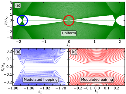
Figure 2: (Color online) (a) Spectrum of uniform $d$-wave SC on a $(1,1)$-edged strip versus momentum $k_{L}$ along the $L$-direction, showing Dirac nodes and zero energy ABSs. Circles indicate regions shown in the next two panels. (b) Formation of flat pseudo-Landau levels near the outer Dirac nodes due to uniform hopping-amplitude gradient in the [1,1] direction; shown here is the near-node region indicated in (a). (c) Similar to (b) but with extended $s$-wave pairing gradient, which induces pseudo-LLs near the central Dirac node indicated in panel (a).

To check the validity of the low-energy linearized Dirac theory, we numerically diagonalized the full lattice Bogoliubov-deGennes (BdG) Hamiltonian using a strip geometry with $(1,1)$ edges (see Fig. 1(b)). The strip width is $W$; the transverse direction, along which periodic boundary conditions were used, has length $L\gg W$. Analogous results for the $(1,0)$-edged strip are presented in Appendix F. We pick a nearest neighbor hopping amplitude $t\!=\!1$, next-neighbor hopping $t^{\prime}\!=\!-0.25t$, electron filling $\bar{n}\!=\!0.85$, and a $d$-wave gap $\Delta_{d}\!=\!0.25t$, such that $v_{\rm f}/v_{\Delta}\!\approx\!13$; these parameters are chosen so as to be representative of the hole-doped cuprate SCs.

Fig. 2(a) shows the spectrum of the $(1,1)$-edged strip as a function of the momentum $k_{L}$ along the long direction $L$, in the absence of any imposed spatial variation for $W\!=\!500\sqrt{2}a_{0}$. The spectrum exhibits $d$-wave Dirac nodes projected onto the Brillouin zone of the strip; the velocity anisotropy $v_{\rm f}/v_{\Delta}\!\gg\!1$ is evident in the dispersion slopes of the outer versus inner nodes. In addition, we find zero energy Andreev bound states (ABSs) expected for a $d$-wave SC in this geometry Kashiwaya and Tanaka (2000); Tsuei and Kirtley (2000); L.öfwander et al. (2001); Deutscher (2005).

Fig. 2(b) shows the spectrum with a nonzero gradient in the hopping amplitude across the strip width, which leads to a pseudo-LL spectrum at the outer Dirac nodes; we have chosen to plot the spectrum near the Dirac node indicated by the circle in Fig. 2(a), for strip width $W\!=\!500\sqrt{2}a_{0}$ and a maximum change $\delta t\!\sim\!0.1t$ at the edge. Fig. 2(c) shows the effect of an extended $s$-wave pairing gradient along the strip width, which leads to pseudo-LL formation at the central Dirac node. Here, we have chosen $W\!=\!2000\sqrt{2}a_{0}$ and a maximum $s$-wave gap $\Delta_{s}\!\sim\!0.4\Delta_{d}$ at the edge. The low energy spectra in Fig. 2(b) and (c) are in quantitative agreement with our analytical results. The spectrum for the $(1,0)$-edged strip (see Appendix F) displays similar strain induced pseudo-LLs; the key difference is in the absence of ABSs for the unstrained $d$-wave SC in this geometry.

V Experimental signature of pseudo-LLs

As in the case of strained graphene, scanning tunneling spectroscopy (STS) experiments which probe the TDOS may provide the most direct route to observing the QP pseudo-LLs. For weak pseudo-magnetic fields, the peaks in density of states due to pseudo-LLs may be visible in microwave spectroscopy. Below, we first provide analytical expressions for the bulk TDOS expected within our continuum low energy theory. We then present numerical results on the lattice model (see Fig. 3) which goes beyond the continuum theory by incorporating the effects of quantum confinement of the Bogoliubov QPs to the strip, as well as the impact of ABSs at the edges.

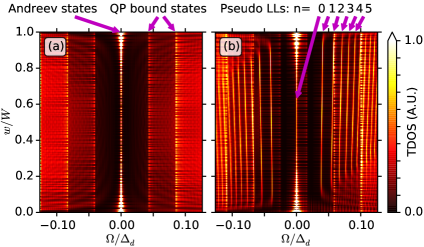
Figure 3: (Color online) Low energy TDOS versus energy $\Omega/\Delta_{d}$ (scaled to the $d$-wave gap), from diagonalization of BdG Hamiltonian in the strip geometry, plotted across scaled strip width $0\!<\!w/W\!<\!1$. (a) Uniform $d$-wave SC, showing ABSs near zero energy localized near $w/W\!=\!0,1$, and QP bound state TDOS exhibiting rapid spatial oscillations. (b) Hopping gradient case showing extra pseudo-LL peaks.

In tunneling experiments, the TDOS in the continuum theory will have two contributions in the bulk. At nodes where the vector potential acts as pure gauge, it will only induce a phase shift for the fermion operators, leading to a TDOS contribution identical to a uniform $d$-wave SC. At nodes where the QPs sense a pseudo-magnetic field, there will be discrete pseudo-LLs. These lead to a total TDOS (details in Appendix D)

$$\!\!N(\Omega) \approx \frac{|\Omega|}{\pi v_{\rm f}v_{\Delta}}\!+\!\frac{|\beta|}{\pi}\sum_{n}\delta(\Omega-\lambda_{n})$$ (10)

where $n=0,\pm 1,\pm 2,\ldots$, and $\lambda_{n}=\sqrt{2\beta v_{\rm f}v_{\Delta}|n|}{\rm sgn}(n)$.

We have also computed the TDOS numerically for the lattice model in the above strip geometry. Confinement to the strip then leads to QP subbands with minima at discrete energies $\sim p\pi v_{\Delta}/W$ and $\sim p\pi v_{\rm f}/W$ for nodes ${{\bf{K}}}_{1},{{\bf{K}}}_{2}$ respectively ($p=$ nonzero integer), as well as ABSs at the strip edges. As seen from Fig. 3, the TDOS for the strip exhibits three key features. (i) Without or with a gradient in the hopping amplitude, we see the zero energy peaks in the TDOS at the top and bottom edges reflecting the presence of ABSs; the spectral weight from these ABSs weakly leaks into the bulk. As shown in Appendix F, the ABSs and their contribution to the TDOS is absent for a (1,0)-edged strip. (ii) In the bulk (i.e., away from the edges), one set of indicated peaks exhibits rapid spatial oscillation of the TDOS across the strip width. These peaks arise when the energy $\Omega$ crosses the minimum $\Omega_{0}^{s}$ (at $k_{L}\!=\!0$) of each subband $s$ in the spectrum, leading to a $\sim\!1/\sqrt{\Omega\!-\!\Omega_{0}^{s}}$ divergence in the TDOS. These QP bound states (see Appendix E) arise due to internode scattering ${{\bf{K}}}_{1}\leftrightarrow-{{\bf{K}}}_{1}$. There are additional weaker features with longer-length-scale spatial variations arising from intranode scattering at $\pm{{\bf{K}}}_{2}$. Both contributions are present even in the absence of a gradient; see Fig. 3(a). (iii) Finally, the hopping gradient induces an extra set of indicated pseudo-LL peaks seen in Fig. 3(b) where the TDOS is nearly constant across the strip. The spatial dependence of the TDOS distinguishes the pseudo-LL peaks from QP bound states.

VI Experimental realizations

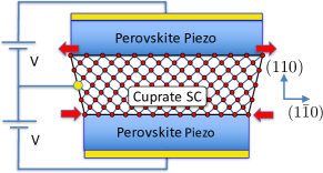
Figure 4: (Color online) Trilayer heterostructure with cuprate SC thin film epitaxially sandwiched between two piezoelectric perovskite films along the $(110)$ surface. An inhomogeneous strain can be induced in the cuprate layer by asymmetrically polarizing the two piezo layers. Metallic outer gates (yellow regions) are used to apply the piezo voltages, with the cuprate layer serving as the common inner gate. For typical values of piezo constant ($d_{31}\!\sim\!50$-$275$pm/V) and dielectric breakdown field ($\sim\!25$MV/m) for piezoelectric perovskites Hooker (1998); Trolier-McKinstry and Muralt (2004) such as Pb(Zr_xTi_1-x)O₃, we estimate that lattice strains $\sim\!0.1$-$1\%$ can be induced in the cuprate layer.

VI.1 Strained nanowires or films

One route to tuning the spatial variation of the electron hopping and pairing amplitudes discussed above is to strain a cuprate thin film or nanowire. Unlike graphene, which has a simple single-particle description of its electronic bands, it is necessary here to include electron interactions in order to study the microscopic impact of strain on the $d$-wave SC. The cuprates may be modelled by a $tJ$ Hamiltonian, $H_{tJ}\!=\!-g_{t}\sum_{i,j,\sigma}t^{\phantom{\dagger}}_{ij}c^{\dagger}_{i\sigma}c^{\phantom{\dagger}}_{j\sigma}\!+\!g_{J}J\sum_{\langle ij\rangle}\vec{S}_{i}\cdot\vec{S}_{j}$, with bare nearest and next-neighbor hoppings $t_{0}$ and $t^{\prime}_{0}\!\approx\!-0.3t_{0}$ respectively, and nearest-neighbor spin exchange $J\!=\!4t_{0}^{2}/U\!\approx 0.3t_{0}$. We set $t_{0}=450$meV which leads to $J=135$meV. The coefficients $g_{t},g_{J}$ represent renormalization factors that crudely account for strong correlation effects. Motivated by slave-boson Kotliar and Liu (1988) and renormalized mean field theory calculations Zhang et al. (1988); Anderson et al. (2004), we pick $g_{t}\!=\!2p/(1\!+\!p)$ and $g_{J}\!=1$, where $p$ is the hole doping (see Appendix G for details). Such a mean field approach captures a variety of experimental observations on the $d$-wave cuprate SCs; we therefore view it as a useful tool to estimate the pseudo-LL gap.

Here, we consider the effects of inhomogeneous strain that can be induced using a piezoelectric thin-film heterostructure schematically depicted and discussed in Fig. 4. Such piezo-induced strain will lead to a gradient in the hopping $\delta t_{0}({{\bf{r}}})$ as well as a change in the superexchange interaction $\delta J({{\bf{r}}})\!\approx\!(8t_{0}/U)\delta t_{0}({{\bf{r}}})$ across the strip. This induces a gradient in the effective hopping and pairing amplitude in the BdG equation. Raman scattering studies of La₂CuO₄ under hydrostatic pressure Aronson et al. (1991) indicate that a $\mp 0.5\%$ change in the lattice constant leads to $\delta J/J\approx\!\pm 5\%$, indirectly implying a change in the bare hopping amplitude $\delta t_{0}/t_{0}\!\approx\!\pm 2.5\%$ in the underlying $tJ$ model. A self-consistent solution to the mean field equations in the SC state at a hole doping $p\!=\!0.15$ shows that such a uniform change leads to a $\approx\!\pm 7\%$ change in the $d$-wave pairing gap and $\approx\!\pm 3\%$ change in the renormalized hopping. A gradient in the $d$-wave gap does not induce any pseudo-LLs; however, the hopping gradient can in fact induce pseudo-LLs as discussed above. For a $(110)$-edged film of thickness $\sim\!700a_{0}$, or a nanowire of similar width ($\approx 270$nm) which is experimentally realizable Bonetti et al. (2004) and similar to the strip geometry explored here, we estimate that a hopping gradient with a realistic $0.5$-$1\%$ maximal strain across the sample will generate a first excited pseudo-LL at $E_{1}\!\sim\!1$meV; this can be probed by $c$-axis tunneling. A fully self-consistent inhomogeneous BdG study of this physics is challenging due to the large system sizes involved; we defer this to future work.

VI.2 Proximity to nematic order

A different route to realizing pseudo-LLs is to note that the onset of nematic order in a tetragonal $d$-wave SC spontaneously breaks the $C_{4}$ point group symmetry and will induce an extended $s$-wave component to the pair field Kim et al. (2008). There is evidence that the cuprates are proximate to such a QPT Hinkov et al. (2008); Daou et al. (2010); Lawler et al. (2010); Sato et al. (2017); Okamoto et al. (2010); Mallik et al. (2016), so that an edge-induced $s$-wave pairing component will exhibit slow spatial decay, leading naturally to a gap variation needed to form pseudo-LLs. Tuning near such a critical point, or using proximity effect coupling to an $s$-wave SC, can tune the decay length and amplitude of the $s$-wave gap, thus controlling the pseudo-magnetic field and permitting further experimental tests.

VII Summary

We have proposed inhomogeneously strained nodal SCs as systems to realize pseudo-gauge fields and pseudo-LLs for Bogoliubov QPs, and suggested experimental routes and signatures to observe such physics in candidate materials such as the cuprate $d$-wave SCs. We note that even accidental SC Dirac nodes will show similar physics. Further research directions include understanding the impact of such inhomogeneous strains on the superconducting transition temperature, its interplay with real magnetic fields and vortices, and extensions to materials like CeCoIn₅, iron pnictides, and candidate topological SCs like Sr₂RuO₄.

Note Added: After submission of our manuscript, a closely related work appeared by Emilian Nica and Marcel Franz (arXiv:1709.01158). Our results, where they overlap, are in agreement.

Appendix A Absence of “scalar gauge potential” in BdG equation

Inhomogeneous strain effects also lead to a deformation potential, which in graphene produces a scalar gauge potential in addition to the pseudo-vector potential Neto et al. (2009); Vozmediano et al. (2010); Lukose et al. (2007); Pacheco Sanjuan et al. (2014); Castro et al. (2016); Naumis et al. (2017). Here, we argue that no such scalar potential – which may significantly alter the low-energy LL structure, or even cause its collapse Castro et al. (2016) – can arise in time-reversal symmetric spin-singlet superconducting systems, such as the one we consider.

The key physical idea is that the BdG Hamiltonian for a singlet SC with time-reversal symmetry only permits 2 of the 4 Pauli matrices – the corresponding coefficients are in fact the two components of the vector potential identified in the main body of the Letter. Thus, any analog of the ‘scalar deformation potential’ here will necessarily break time-reversal symmetry or lead to singlet-triplet mixing. Such terms will be allowed in a more general setting, for example if spin orbit coupling is present and inversion symmetry or time-reversal symmetry is broken, but not in the cases studied here.

The Pauli matrix components that can enter the Hamiltonian of Equation 4 of the manuscript are constrained by symmetry. This is most easily seen by considering the BdG Hamiltonian in real space,

$$H_{\text{BdG}}=\sum_{i,j}\psi^{\dagger}_{i}h^{\vphantom{\dagger}}_{ij}\psi^{\vphantom{\dagger}}_{j},$$ (11)

$$h_{ij}=\begin{pmatrix}d^{0}_{ij}+d^{3}_{ij}&\Delta_{ij}\\ \Delta_{ji}^{*}&d^{0}_{ij}-d^{3}_{ij}\end{pmatrix},$$ (12)

where $\psi_{i}^{\dagger}=(c^{\dagger}_{i\uparrow},c^{\vphantom{\dagger}}_{i\downarrow})$ is the Nambu spinor at site $i$, and $d^{0}_{ij},d^{3}_{ij},\Delta_{ij}$ are complex numbers, with hermiticity imposing the constraint that $d^{0}_{ij}=(d^{0}_{ji})^{*}$ and $d^{3}_{ij}=(d^{3}_{ji})^{*}$.

• Time-reversal symmetry, which sends $c_{i\uparrow}\to c_{i\downarrow}$, $c_{i\downarrow}\to-c_{i\uparrow}$, and complex-conjugates all complex numbers, leads to the additional restrictions (i) $d^{0}_{ij}=0$ and (ii) $\Delta_{ij}=\Delta_{ji}^{*}$.

• Spin rotation symmetry and singlet pairing further imposes the constraints $d^{3}_{ij}=(d^{3}_{ij})^{*}$ and $\Delta_{ij}=\Delta_{ij}^{*}$.

With these ingredients, the Hamiltonian matrix $h_{ij}=d^{3}_{ij}\sigma^{3}+\Delta_{ij}\sigma^{1}$, where $d^{3}_{ij}$ and $\Delta_{ij}$ are real numbers. Thus, time-reversal symmetry and spin-rotation symmetry respectively require that the coefficients of $\sigma^{0}$ (which corresponds to a valley-odd chemical potential) and $\sigma^{2}$ (which corresponds to a complex pairing component) both vanish.

Such a Hamiltonian captures a BdG SC with arbitrary spatial modulations in hopping and pairing amplitudes, and an appropriate low-energy ‘Dirac node’ expansion recovers Equation 4 of our manuscript, and only permits the two components of the vector potential which we have shown leads to the formation of pseudo-LLs. Any additional ‘scalar potential’ is thus symmetry forbidden. Breaking such symmetries, for instance with a supercurrent that breaks time-reversal symmetry, leads to a Doppler shift for the QPs, which is an analog of a ‘scalar potential’.

Appendix B Dirac BdG solution - gap variations

Start with the Hamiltonian at node $\ell=1$ for the case discussed in the main text where pseudo-LLs arise from gap variations.

$$H=\left[\!-iv_{\rm f}\sigma^{z}\partial_{x}\!+\!\beta v_{\Delta}\sigma^{x}(x\!-\!\frac{k}{\beta})\!\right]$$ (13)

Note that $({\rm sgn}\beta~{}\sigma^{y})$ anticommutes with this Hamiltonian, so that if $\ket{\Phi}$ is an eigenstate of $H$ with energy $E$, then $({\rm sgn}\beta~{}\sigma^{y})\ket{\Phi}$ is a solution with energy $-E$. (Here, ${\rm sgn}\beta=\beta/|\beta|$), This is the BdG particle-hole symmetry. Let us define

$$-i\partial_{x} = i\sqrt{\frac{|\beta|v_{\Delta}}{2v_{\rm f}}}(a^{\dagger}-a^{\phantom{\dagger}})$$ (14)

$$(x-\frac{k}{\beta}) = \sqrt{\frac{v_{\rm f}}{2|\beta|v_{\Delta}}}(a^{\dagger}+a^{\phantom{\dagger}})$$ (15)

so we get

$$\!\!\!H=\sqrt{2|\beta|v_{\rm f}v_{\Delta}}\left[a^{\dagger}\frac{(\sigma^{x}{\rm sgn}\beta+i\sigma^{z})}{2}+a^{\phantom{\dagger}}\frac{(\sigma^{x}{\rm sgn}\beta-i\sigma^{z})}{2}\right]$$ (16)

Define spinors

$$\ket{\uparrow}\equiv\frac{1}{\sqrt{2}}\begin{pmatrix}1\\ i~{}{\rm sgn}\beta\end{pmatrix};\ket{\downarrow}\equiv\frac{1}{\sqrt{2}}\begin{pmatrix}1\\ -i~{}{\rm sgn}\beta\end{pmatrix}$$ (17)

Then Hamiltonian is of the Jaynes-Cummings type,

$$H=\sqrt{2|\beta|v_{\rm f}v_{\Delta}}\left[ia^{\dagger}{\cal S}^{-}-ia{\cal S}^{+}\right]$$ (18)

where ${\cal S}^{\pm}$ act as raising/lowering operators on the above spin-$1/2$ states. Let $\ket{n}$ denote harmonic oscillator states (with $n\geq 0$) centered at $k/\beta$ which are generated by $a,a^{\dagger}$. Then, we have a zero energy eigenstate

$$\ket{\Phi_{0}}=\ket{0}\ket{\downarrow}$$ (19)

and nonzero energy solutions

$$\ket{\Phi_{n\pm}} = \frac{\ket{n-1}\ket{\uparrow}\pm i\ket{n}\ket{\downarrow}}{\sqrt{2}}$$ (20)

with respective energies $\pm\sqrt{2|\beta|v_{\rm f}v_{\Delta}n}$. More explicitly, the wavefunctions are given by

$$\Phi_{k0}(x) = \frac{1}{\sqrt{2}}\varphi_{0}(x-\frac{k}{\beta})\begin{pmatrix}1\\ -i{\rm sgn}\beta\end{pmatrix}$$ (21)

$$\Phi_{kn\pm}(x) = \frac{1}{2}\begin{pmatrix}\varphi_{n-1}(x-\frac{k}{\beta})\pm i\varphi_{n}(x-\frac{k}{\beta})\\ {\rm sgn}\beta(i\varphi_{n-1}(x-\frac{k}{\beta})\pm\varphi_{n}(x-\frac{k}{\beta}))\end{pmatrix}$$ (22)

where $\varphi_{n}(x)$ is the $n^{\rm th}$ harmonic oscillator ground state. We can then define quasiparticle operators $\gamma$ for the node pair $\ell=\pm 1$, so that

$$\Psi_{1\alpha}({{\bf{r}}})=\begin{pmatrix}\psi_{1,\alpha}({{\bf{r}}})\\ \epsilon^{\phantom{\dagger}}_{\alpha\nu}\psi^{\dagger}_{-1,\nu}({{\bf{r}}})\end{pmatrix}=\frac{1}{\sqrt{L}}\sum_{k}{\rm e}^{iky}\left[\gamma_{0,\alpha}(k)\Phi_{k0}(x)+\sum_{n>0}\begin{pmatrix}\Phi_{kn+}(x)&\Phi_{kn-}(x)\end{pmatrix}\begin{pmatrix}\gamma_{n,1,\alpha}(k)\\ \epsilon^{\phantom{\dagger}}_{\alpha\nu}\gamma^{\dagger}_{n,-1,\nu}(-k)\end{pmatrix}\right]$$ (23)

In terms of these, the Hamiltonian is given by

$$H=\sum_{k,\alpha,n>0}\sqrt{2|\beta|v_{\rm f}v_{\Delta}n}\left(\gamma^{\dagger}_{n1\alpha}(k)\gamma^{\phantom{\dagger}}_{n1\alpha}(k)+\gamma^{\dagger}_{n2\alpha}(k)\gamma^{\phantom{\dagger}}_{n2\alpha}(k)\right)$$ (24)

Appendix C Dirac BdG solution - hopping variations

Start with the Hamiltonian at node $\ell=2$ for the case discussed in the main text where pseudo-LLs arise from hopping variations. Assume plane waves along the $x$-direction. Then

$$H=\beta v_{\rm f}\sigma^{z}(y+\frac{k}{\beta})\!-\!iv_{\Delta}\sigma^{x}\partial_{y}$$ (25)

Let us define

$$-i\partial_{y} = i\sqrt{\frac{|\beta|v_{\rm f}}{2v_{\Delta}}}(a^{\dagger}-a^{\phantom{\dagger}})$$ (26)

$$(y+\frac{k}{\beta}) = \sqrt{\frac{v_{\Delta}}{2|\beta|v_{\rm f}}}(a^{\dagger}+a^{\phantom{\dagger}})$$ (27)

so we get

$$\!\!\!H=\sqrt{2|\beta|v_{\rm f}v_{\Delta}}\left[a^{\dagger}\frac{(\sigma^{z}{\rm sgn}\beta+i\sigma^{x})}{2}+a^{\phantom{\dagger}}\frac{(\sigma^{z}{\rm sgn}\beta-i\sigma^{x})}{2}\right]$$ (28)

Define spinors

$$\ket{\uparrow}\equiv\frac{1}{\sqrt{2}}\begin{pmatrix}1\\ -i~{}{\rm sgn}\beta\end{pmatrix};\ket{\downarrow}\equiv\frac{1}{\sqrt{2}}\begin{pmatrix}1\\ i~{}{\rm sgn}\beta\end{pmatrix}$$ (29)

Then Hamiltonian is of the Jaynes-Cummings type,

$$H=\sqrt{2|\beta|v_{\rm f}v_{\Delta}}\left[ia^{\dagger}{\cal S}^{-}-ia{\cal S}^{+}\right]$$ (30)

where ${\cal S}^{\pm}$ act as raising/lowering operators on the above spin-$1/2$ states. Let $\ket{n}$ denote harmonic oscillator states (with $n\geq 0$) centered at $y=-k/\beta$ which are generated by $a,a^{\dagger}$. Then, we have a zero energy eigenstate

$$\ket{\Phi_{0}}=\ket{0}\ket{\downarrow}$$ (31)

and nonzero energy solutions

$$\ket{\Phi_{n\pm}} = \frac{\ket{n-1}\ket{\uparrow}\pm i\ket{n}\ket{\downarrow}}{\sqrt{2}}$$ (32)

with respective energies $\pm\sqrt{2|\beta|v_{\rm f}v_{\Delta}n}$. More explicitly, the wavefunctions are given by

$$\Phi_{k0}(y) = \frac{1}{\sqrt{2}}\varphi_{0}(y+\frac{k}{\beta})\begin{pmatrix}1\\ i{\rm sgn}\beta\end{pmatrix}$$ (33)

$$\Phi_{kn\pm}(y) = \frac{1}{2}\begin{pmatrix}\varphi_{n-1}(y+\frac{k}{\beta})\pm i\varphi_{n}(y+\frac{k}{\beta})\\ -{\rm sgn}\beta(i\varphi_{n-1}(y+\frac{k}{\beta})\pm\varphi_{n}(y+\frac{k}{\beta}))\end{pmatrix}$$ (34)

where $\varphi_{n}(y)$ is the $n^{\rm th}$ harmonic oscillator ground state.

Appendix D Tunneling density of states (TDOS)

D.1 Uniform case

The superconducting local TDOS for spin-$\alpha$ for a uniform $d$-wave SC is given by

$$N_{\alpha}({{\bf{r}}},\Omega)=\int\frac{d^{2}{{\bf{k}}}}{(2\pi)^{2}}\left[u^{2}_{{\bf{k}}}\delta(\Omega-E_{{\bf{k}}})+v^{2}_{{\bf{k}}}\delta(\Omega+E_{{\bf{k}}})\right]$$ (35)

where $u_{{\bf{k}}}^{2}=\frac{1}{2}(1+\xi_{{\bf{k}}}/E_{{\bf{k}}})$, $v_{{\bf{k}}}^{2}=\frac{1}{2}(1-\xi_{{\bf{k}}}/E_{{\bf{k}}})$, and $E_{{\bf{k}}}=\sqrt{\xi^{2}_{{\bf{k}}}+\Delta^{2}_{{\bf{k}}}}$. We can linearize the dispersion around the 4 nodes (labelled $\ell=\pm 1,\pm 2$), which leads to

$$N_{\alpha}({{\bf{r}}},\Omega)=\sum_{\ell}\int^{\Lambda}\frac{d^{2}q}{(2\pi)^{2}}\frac{1}{2}\left[(1+\frac{\vec{v}_{\rm f}^{(\ell)}\cdot\vec{q}}{\cal E_{\bf{q}}})\delta(\Omega-{\cal E_{\bf{q}}})+(1-\frac{\vec{v}_{\rm f}^{(\ell)}\cdot\vec{q}}{\cal E_{\bf{q}}})\delta(\Omega+{\cal E_{\bf{q}}})\right]$$ (36)

where ${\cal E}_{\bf{q}}=\sqrt{v_{\rm f}^{2}q_{\perp}^{2}+v_{\Delta}^{2}q_{\parallel}^{2}}$ and the momentum cutoff $\Lambda$ ensures the same total number of momentum states. Doing the integral, we find

$$N_{\alpha}({{\bf{r}}},\Omega)=2\int^{\Lambda}\frac{dq_{\parallel}dq_{\perp}}{(2\pi)^{2}}\left[\delta(\Omega-\sqrt{v_{\rm f}^{2}q_{\perp}^{2}+v_{\Delta}^{2}q_{\parallel}^{2}})+\delta(\Omega+\sqrt{v_{\rm f}^{2}q_{\perp}^{2}+v_{\Delta}^{2}q_{\parallel}^{2}})\right]$$ (37)

Rescaling $v_{\rm f}q_{\parallel}=Q_{1}$ and $v_{\Delta}q_{\perp}=Q_{2}$, with $Q=\sqrt{Q^{2}_{1}+Q^{2}_{2}}$, we find

$$N_{\alpha}({{\bf{r}}},\Omega)=2\int^{\Lambda}\frac{dQ}{2\pi v_{\rm f}v_{\Delta}}Q\left[\delta(\Omega-Q)+\delta(\Omega+Q)\right]$$ (38)

with an appropriate choice $\Lambda=\sqrt{\pi v_{\rm f}v_{\Delta}}$. Of course, this linearized description will break down at a lower energy scale $\sim v_{\Delta}/a_{0}$, where $a_{0}$ is the lattice spacing. This yields, for $|\Omega|\lesssim v_{\Delta}/a_{0}\ll\Lambda$,

$$N({{\bf{r}}},\Omega)=\sum_{\alpha}N_{\alpha}({{\bf{r}}},\Omega)=\frac{2|\Omega|}{\pi v_{\rm f}v_{\Delta}}$$ (39)

D.2 Pseudo-Landau Level case: Gap variations

Consider the gap variation example discussed in the main text. Then, fermions at two of the Dirac points only see a phase change from the vector potential, which does not change the density of states, leading to a contribution from $\ell=\pm 2$ given by

$$N_{2}({{\bf{r}}},\Omega)=\frac{|\Omega|}{\pi v_{\rm f}v_{\Delta}}.$$ (40)

This is half the total density of states in the uniform case. The contribution from the other node pair $N_{1}({{\bf{r}}},\Omega)$ is expected to reflect the formation of pseudo-LLs. The Green function for node pair $\ell=\pm 1$ reduces to

$${\cal G}_{\alpha}^{(\ell=1)}({{\bf{r}}},i\Omega_{m})=\frac{1}{2L}\sum_{k}\left[\frac{\varphi^{2}_{0}(x-\frac{k}{\beta})}{i\Omega_{m}-E_{0}}+\frac{1}{2}\sum_{n>0}\left(\varphi^{2}_{n}(x-\frac{k}{\beta})+\varphi^{2}_{n-1}(x-\frac{k}{\beta})\right)\left(\frac{1}{i\Omega_{m}-E_{n}}+\frac{1}{i\Omega_{m}+E_{n}}\right)\right]$$ (41)

where $E_{0}=0$. Summing over spins and $\ell=\pm 1$, this leads to

$$N_{1}({{\bf{r}}},\Omega)=\frac{2}{L}\sum_{k}\left[\varphi_{0}^{2}(x-\frac{k}{\beta})\delta(\Omega)+\frac{1}{2}\sum_{n>0}\left(\varphi^{2}_{n}(x-\frac{k}{\beta})+\varphi^{2}_{n-1}(x-\frac{k}{\beta})\right)\left(\delta(\Omega-E_{n})+\delta(\Omega+E_{n})\right)\right]$$ (42)

Deep in the bulk, $N_{1}({{\bf{r}}},\Omega)$ will be independent of ${{\bf{r}}}$, and we can approximate it as

$$N_{1}({{\bf{r}}},\Omega)\approx\frac{|\beta|}{\pi}\left[\delta(\Omega)+\sum_{n>0}\left(\delta(\Omega-E_{n})+\delta(\Omega+E_{n})\right)\right]$$ (43)

which can be recast in the more compact form

$$N_{1}({{\bf{r}}},\Omega)\approx\frac{|\beta|}{\pi}\sum_{n}\delta(\Omega-\lambda_{n})$$ (44)

where $n=0,\pm 1,\pm 2,\ldots$, with $\lambda_{n}=\sqrt{2\beta v_{\rm f}v_{\Delta}|n|}{\rm sgn}(n)$. Thus, the total density of states, $N_{1}({{\bf{r}}},\Omega)+N_{2}({{\bf{r}}},\Omega)$ will reflect a combination of the pseudo-LL spectrum as well as the Dirac density of states of the uniform $d$-wave SC.

Appendix E Appendix E. d-wave SC in a narrow strip

In this section we study singular contributions to the TDOS which come from quantization of the quasiparticle momentum transverse to the strip. Just in this section, we find it convenient to retain the full BdG equation, and linearize around the Dirac nodes only at the end. We begin with the BdG Hamiltonian,

$$\hat{H}(k_{L})=\left(\begin{array}[]{cc}\xi(k_{L},-i\partial_{w})&\Delta(k_{L},-i\partial_{w})\\ \Delta(k_{L},-i\partial_{w})&-\xi(k_{L},-i\partial_{w})\end{array}\right),$$ (45)

where $0<w<W$ is the transverse coordinate, and $k_{L},k_{W}$ will denote momenta along the strip length and strip width ($L$, $W$ directions) respectively. For a $(110)$ edge, we have $\xi(k_{L},-k_{W})=\xi(k_{L},k_{W})$ and $\Delta(k_{L},-k_{W})=-\Delta(k_{L},k_{W})$. We are looking for states which obey the strip boundary conditions, i.e., eigenfunctions, $\psi(w)$, of $\hat{H}$ which have a vanishing charge density at the strip edges, $\psi^{\dagger}(0)\tau^{z}\psi(0)=\psi^{\dagger}(W)\tau^{z}\psi(W)=0$. A plane wave eigenfunction with positive eigenvalue $\varepsilon(k_{L},k_{W})=\sqrt{\xi^{2}(k_{L},k_{W})+\Delta^{2}(k_{L},k_{W})}$ is given by

$$\phi^{+}(k_{L},k_{W};w)=\left(\begin{array}[]{c}u(k_{L},k_{W})\\ v(k_{L},k_{W})\end{array}\right)e^{ik_{W}w},$$ (46)

where

$$|u(k_{L},k_{W})|^{2}=\frac{1}{2}\left(1+\frac{\xi(k_{L},k_{W})}{\varepsilon(k_{L},k_{W})}\right),$$ (47)

and

$$|v(k_{L},k_{W})|^{2}=\frac{1}{2}\left(1-\frac{\xi(k_{L},k_{W})}{\varepsilon(k_{L},k_{W})}\right).$$ (48)

Since $\Delta(k_{L},k_{W})$ is a real function for the $d$-wave SC we are considering, it is sufficient to take $u(k_{L},k_{W})>0$ and $({\rm sign~{}}v(k_{L},k_{W}))=({\rm sign~{}}\Delta(k_{L},k_{W}))$, thus, $u(k_{L},-k_{W})=u(k_{L},k_{W})$ and $v(k_{L},-k_{W})=-v(k_{L},k_{W})$. A plane wave eigenfunction with negative energy $-\varepsilon(k_{L},k_{W})$ is given by

$$\phi^{-}(k_{L},k_{W};w)=\left(\begin{array}[]{c}v(k_{L},k_{W})\\ -u(k_{L},k_{W})\end{array}\right)e^{ik_{W}w}.$$ (49)

To construct a state which obeys the boundary conditions, we consider a superposition of states with opposite $k_{W}$,

$$\psi^{+}(k_{L},k_{W}>0,w) = \phi^{+}(k_{L},k_{W},w)+r(k_{L},k_{W})\phi^{+}(k_{L},-k_{W})$$ (54)

$$= \left(\begin{array}[]{c}u(k_{L},k_{W})\\ v(k_{L},k_{W})\end{array}\right)e^{ik_{W}w}+r(k_{L},k_{W})\left(\begin{array}[]{c}u(k_{L},k_{W})\\ -v(k_{L},k_{W})\end{array}\right)e^{-ik_{W}w}.$$

The charge density for this state is given by (dependence on $k_{L}$ and $k_{W}$ implicit)

$$\rho^{+}(w) = \psi^{+\dagger}(w)\tau^{z}\psi^{+}(w).\$$ (56)

$$= u^{2}(1+|r|^{2}+2\Re(re^{-i2k_{W}w}))-v^{2}(1+|r|^{2}-2\Re(re^{-i2k_{w}W}))$$

$$= (u^{2}-v^{2})(1+|r|^{2})+2\Re(re^{-i2k_{W}w}),$$

where $\Re(z)$ denotes the real part of $z$. Finite size quantization sets as usual $k_{W}=\pi n/W$, where $n=0,1,2...$, while demanding that $\rho^{+}$ vanish at the strip edges results in

$$(u^{2}-v^{2})(1+|r|^{2})+2\Re(r)=0.$$ (57)

Since, $-1\leq u^{2}-v^{2}\leq 1$, $r$ is always real. Thus, the eigenstates are given by

$$\psi_{n}^{+}(k_{L};w) = \left(\begin{array}[]{c}u_{n}(k_{L})\\ v_{n}(k_{L})\end{array}\right)e^{i\pi nw/W}+r_{n}(k_{L})\left(\begin{array}[]{c}u_{n}(k_{L})\\ -v_{n}(k_{L})\end{array}\right)e^{-i\pi nw/W}.$$ (62)

Similar states with negative energy are given by

$$\psi_{n}^{-}(k_{L};w) = \left(\begin{array}[]{c}v_{n}(k_{L})\\ -u_{n}(k_{L})\end{array}\right)e^{i\pi nw/W}+r_{n}(k_{L})\left(\begin{array}[]{c}-v_{n}(k_{L})\\ -u_{n}(k_{L})\end{array}\right)e^{-i\pi nw/W}.$$ (67)

The TDOS is given by

$$N(\Omega,w)=\frac{1}{2}\int\frac{dk_{L}}{2\pi}\sum_{n=0}^{\infty}\sum_{s=\pm}\psi^{s\dagger}_{n}(k_{L},w)(\tau^{0}+s\tau^{z})\psi^{s}_{n}(k_{L},w)\delta(\Omega-s\varepsilon_{n}(k_{L}))$$ (68)

Focusing on positive energies,

$$N(\Omega>0,w)=2\int\frac{dk_{L}}{2\pi}\sum_{n}u_{n}^{2}(k_{L})\left(1+r_{n}^{2}(k_{L})+2r_{n}(k_{L})\cos\frac{\pi nw}{W}\right)\delta(\Omega-\varepsilon_{n}(k_{L}))$$ (69)

The main low energy contributions to the TDOS in a $d$-wave SC come from the vicinity of the nodes. We are further focusing on the nodes at $k_{L}=0$ and $k_{W}=\pm K_{F}$, thus, for $k_{W}>0$, $\xi\simeq v_{\rm f}(n\pi/W-K_{F})$, $\Delta\simeq v_{\Delta}k_{L}$, and $\varepsilon\simeq\sqrt{v_{\rm f}^{2}(n\pi/W-K_{F})^{2}+v_{\Delta}^{2}k_{L}^{2}}$. Changing integration variables we have

$$N(\Omega>0,w) = 2\int_{v_{\rm f}|n\pi/W-K_{F}|}^{\infty}\frac{\varepsilon d\varepsilon}{2\pi}\sum_{n}\frac{1}{v_{\Delta}k_{n}(\varepsilon)}u_{n}^{2}(\varepsilon)\left(1+r_{n}^{2}+2r_{n}\cos\frac{\pi nw}{W}\right)\delta(\Omega-\varepsilon)$$ (70)

$$= \sum_{n}\Theta(\Omega-v_{\rm f}|n\pi/W-K_{F}|)\frac{\Omega}{\pi}\frac{1}{v_{\Delta}k_{n}(\Omega)}u_{n}^{2}(\Omega)\left(1+r_{n}^{2}+2r_{n}\cos\frac{\pi nw}{W}\right),$$

where $k_{n}(\Omega)=\sqrt{\Omega^{2}-(v_{\rm f}n\pi/w-K)^{2}}/v_{\Delta}$, and $u_{n}^{2}(\Omega)=(1+v_{\rm f}(n\pi/w-K_{F})/\Omega)/2$. Since there are always values of $w$ for which the term in the above parentheses is finite, we find that there are contributions at $\Omega=v_{\rm f}|n\pi/W-K_{F}|$ which diverge as $1/\sqrt{\Omega^{2}-(v_{\rm f}n\pi/W-K_{F})^{2}}$.

Appendix F Appendix F. Pseudo-Landau levels of strained d-wave SC in the (1,0)-edged strip geometry

Numerical diagonalization of the lattice BdG Hamiltonian was also performed for a $(1,0)$-edged strip. Again, the strip’s width is $W$, and the transverse direction, along which periodic boundary conditions were used, has length $L\gg W$. Parameters $t$, $t^{\prime}$, $\bar{n}$, and $\Delta_{d}$ are taken to be the same as in the $(1,1)$-edged case considered in the main text.

Fig. 5(a) shows the spectrum of the strip as a function of the momentum $k_{L}$ along the long direction $L$ in the absence of any imposed spatial variation. The spectrum exhibits the $d$-wave Dirac nodes projected onto the Brillouin zone of the strip. As expected with $(1,0)$ edges, zero-energy ABSs are absent from the spectrum. A circle indicates the near-node region in which we have chosen to plot the spectra of panels (b) and (c).

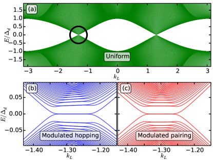
Figure 5: (Color online) (a) Spectrum of uniform $d$-wave SC on a $(1,0)$-edged strip versus momentum $k_{L}$ along the $L$-direction showing Dirac nodes. Note that there are no zero energy ABSs in this geometry. Circle indicates region shown in the next two panels. (b) Formation of flat pseudo-Landau levels in the low-energy regime due to uniform hopping-amplitude gradient in the $[1,0]$ direction; shown here is the near-node region indicated in (a). (c) Similar to (b) but with extended $s$-wave pairing gradient.

Fig. 5(b) shows the spectrum in the presence of a nonzero gradient in the hopping amplitude across the strip width (in the $[1,0]$ direction), which leads to a pseudo-LL spectrum at both Dirac nodes; we have chosen $W\!=\!3000a_{0}$ and a maximum change $\delta t\!\sim\!0.25t$ at the edge. Fig. 5(c) shows the effect of an extended $s$-wave pairing gradient across the strip width, also leading to pseudo-LL formation at both Dirac nodes. Here, we have chosen $W\!=\!3000a_{0}$ and a maximum $s$-wave gap $\Delta_{s}\!\sim\!0.25\Delta_{d}$ at the edge. The low energy spectra in Fig. 5(b) and (c) are in quantitative agreement with our analytical results.

Appendix G Appendix G. Mean field equations for correlated d-wave SC with strain

We start from the usual $tJ$ model in the main text

$$H_{tJ}=-g_{t}\sum_{i,j,\alpha}t_{0,ij}c^{\dagger}_{i\alpha}c^{\phantom{\dagger}}_{j\alpha}+g_{J}J\sum_{\langle ij\rangle}\vec{S}_{i}\cdot\vec{S}_{j}$$ (71)

where the bare nearest neighbor and next-neighbor hoppings are $t_{0}=1$ and $t^{\prime}_{0}=-0.3t_{0}$ respectively, the antiferromagnetic exchange coupling $J=4t_{0}^{2}/U=0.3t_{0}$, and the renormalization factors $g_{t}=2p/(1+p)$, $g_{J}=1$ account for strong correlation effects in a mean field manner. Note that $g_{t}$ is chosen in line with renormalized mean field theory, while we have set $g_{J}=1$ similar to what one expects from slave boson mean field theory. At any rate, we should only view this as an effective model to obtain a variational $d$-wave superconducting ground state, with results which approximately reproduce experimental data. Doing a full Hartree-Fock-Bogoliubov mean field theory of the superexchange term, we arrive at the mean field Hamiltonian

$$H_{\rm MFT}=\sum_{{{\bf{k}}}\alpha}\xi^{\phantom{\dagger}}_{{\bf{k}}}c^{\dagger}_{{{\bf{k}}}\alpha}c^{\phantom{\dagger}}_{{{\bf{k}}}\alpha}-\sum_{{\bf{k}}}\Delta^{\phantom{\dagger}}_{{\bf{k}}}(c^{\dagger}_{{{\bf{k}}}\uparrow}c^{\dagger}_{-{{\bf{k}}}\downarrow}+c^{\phantom{\dagger}}_{-{{\bf{k}}}\downarrow}c^{\phantom{\dagger}}_{{{\bf{k}}}\uparrow}),$$ (72)

where $\xi_{{\bf{k}}}=-2(g_{t}t_{0}+\frac{3}{4}g_{J}J\chi)(\cos k_{x}+\cos k_{y})-4g_{t}t_{0}^{\prime}\cos k_{x}\cos k_{y}$ is set by the effectively renormalized hoppings (which appear in our BdG calculations in the paper), $t=(g_{t}t_{0}+\frac{3}{4}g_{J}J\chi)$ and $t^{\prime}=g_{t}t_{0}^{\prime}$, while the pairing gap $\Delta_{{\bf{k}}}=\frac{3}{2}g_{J}J\Delta_{0}(\cos k_{x}-\cos k_{y})$. The mean field equations determining $\chi,\Delta_{0}$ and the mean electron density $\bar{n}\equiv 1-p$ are given by

$$\Delta_{0} = \frac{1}{2N}\sum_{{\bf{k}}}\frac{\Delta_{{\bf{k}}}}{2E_{{\bf{k}}}}(\cos k_{x}-\cos k_{y})$$ (73)

$$\chi = \frac{1}{4N}\sum_{{\bf{k}}}(1-\frac{\xi_{{\bf{k}}}}{E_{{\bf{k}}}})(\cos k_{x}+\cos k_{y})$$ (74)

$$\bar{n} = \frac{1}{N}\sum_{{\bf{k}}}(1-\frac{\xi_{{\bf{k}}}}{E_{{\bf{k}}}})\equiv 1-p$$ (75)

where $E_{{\bf{k}}}=\sqrt{\xi_{{\bf{k}}}^{2}+\Delta_{{\bf{k}}}^{2}}$. We solve these equations self-consistently assuming $t_{0}\to t_{0}(1+\varepsilon)$ and $J\to J(1+2\varepsilon)$, where the (small) fractional change $\varepsilon$ in the hopping and exchange interaction is determined by the strain which affects the lattice constant; see main text. (The factor of $2\varepsilon$ in $J$ reflects its dependence on hopping as $\sim\!t_{0}^{2}$.)

We pick the bare hopping $t_{0}=450$meV, which leads to $J=135$meV (corresponding to $U/t_{0}\!\approx\!13$). For hole doping $p=0.15$, and for the unstrained case $\varepsilon=0$, we find that the renormalized hoppings satisfy $t^{\prime}=-0.25t$, and an anti-nodal gap $3g_{J}J\Delta_{0}\approx 24$meV at $(\pi,0)$. In addition, with the lattice constant $a_{0}=3.85$Å, we find a nodal Fermi velocity $v_{\rm f}\approx 1.3$eV-Å, and a ratio of Fermi velocity to gap velocity $v_{\rm f}/v_{\Delta}\approx 20$. These are in reasonable agreement with results for the optimally doped cuprates. Incorporating $\varepsilon$, and solving the mean field equations, we find the results for the strain dependence of the hopping and pairing quoted in the main text.

References

- Amorim et al. (2016) B. Amorim, A. Cortijo, F. de Juan, A. G. Grushin, F. Guinea, A. Gutiérrez-Rubio, H. Ochoa, V. Parente, R. Roldán, P. San-Jose, J. Schiefele, M. Sturla, and M. A. H. Vozmediano, “Novel effects of strains in graphene and other two dimensional materials,” Physics Reports 617, 1 – 54 (2016).
- Neto et al. (2009) A. H. Castro Neto, F. Guinea, Nuno M. R. Peres, Kostya S. Novoselov, and Andre K. Geim, “The electronic properties of graphene,” Reviews of Modern Physics 81, 109 (2009).
- Guinea et al. (2010) F. Guinea, M. I. Katsnelson, and A. K. Geim, “Energy gaps and a zero-field quantum hall effect in graphene by strain engineering,” Nat Phys 6, 30–33 (2010).
- Vozmediano et al. (2010) María A. H. Vozmediano, M. I. Katsnelson, and Francisco Guinea, “Gauge fields in graphene,” Physics Reports 496, 109–148 (2010).
- Levy et al. (2010) N. Levy, S. A. Burke, K. L. Meaker, M. Panlasigui, A. Zettl, F. Guinea, A. H. Castro Neto, and M. F. Crommie, “Strain-induced pseudo–magnetic fields greater than 300 tesla in graphene nanobubbles,” Science 329, 544–547 (2010).
- Gomes et al. (2012) Kenjiro K. Gomes, Warren Mar, Wonhee Ko, Francisco Guinea, and Hari C. Manoharan, “Designer Dirac fermions and topological phases in molecular graphene,” Nature 483, 306–310 (2012).
- Zeljkovic et al. (2015) Ilija Zeljkovic, Daniel Walkup, Badih A. Assaf, Kane L. Scipioni, R. Sankar, Fangcheng Chou, and Vidya Madhavan, “Strain engineering Dirac surface states in heteroepitaxial topological crystalline insulator thin films,” Nat. Nano. 10, 849–853 (2015).
- Liu et al. (2016) Jian Liu, D. Kriegner, L. Horak, D. Puggioni, C. Rayan Serrao, R. Chen, D. Yi, C. Frontera, V. Holy, A. Vishwanath, J. M. Rondinelli, X. Marti, and R. Ramesh, “Strain-induced nonsymmorphic symmetry breaking and removal of Dirac semimetallic nodal line in an orthoperovskite iridate,” Phys. Rev. B 93, 085118 (2016).
- Ochi et al. (2016) Masayuki Ochi, Ryotaro Arita, Nandini Trivedi, and Satoshi Okamoto, “Strain-induced topological transition in SrRu2O6 and CaOs2O6,” Phys. Rev. B 93, 195149 (2016).
- Zhu et al. (2016) Liyan Zhu, Shan-Shan Wang, Shan Guan, Ying Liu, Tingting Zhang, Guibin Chen, and Shengyuan A. Yang, “Blue phosphorene oxide: Strain-tunable quantum phase transitions and novel 2D emergent fermions,” Nano Letters 16, 6548–6554 (2016), pMID: 27648670.
- Rayan Serrao et al. (2013) C. Rayan Serrao, Jian Liu, J. T. Heron, G. Singh-Bhalla, A. Yadav, S. J. Suresha, R. J. Paull, D. Yi, J.-H. Chu, M. Trassin, A. Vishwanath, E. Arenholz, C. Frontera, J. Železný, T. Jungwirth, X. Marti, and R. Ramesh, “Epitaxy-distorted spin-orbit Mott insulator in Sr2IrO4 thin films,” Phys. Rev. B 87, 085121 (2013).
- Lupascu et al. (2014) A. Lupascu, J. P. Clancy, H. Gretarsson, Zixin Nie, J. Nichols, J. Terzic, G. Cao, S. S. A. Seo, Z. Islam, M. H. Upton, Jungho Kim, D. Casa, T. Gog, A. H. Said, Vamshi M. Katukuri, H. Stoll, L. Hozoi, J. van den Brink, and Young-June Kim, “Tuning magnetic coupling in Sr2IrO4 thin films with epitaxial strain,” Phys. Rev. Lett. 112, 147201 (2014).
- Choi et al. (2004) K. J. Choi, M. Biegalski, Y. L. Li, A. Sharan, J. Schubert, R. Uecker, P. Reiche, Y. B. Chen, X. Q. Pan, V. Gopalan, L.-Q. Chen, D. G. Schlom, and C. B. Eom, “Enhancement of ferroelectricity in strained BaTiO3 thin films,” Science 306, 1005–1009 (2004).
- Hicks et al. (2014) Clifford W. Hicks, Daniel O. Brodsky, Edward A. Yelland, Alexandra S. Gibbs, Jan A. N. Bruin, Mark E. Barber, Stephen D. Edkins, Keigo Nishimura, Shingo Yonezawa, Yoshiteru Maeno, et al., “Strong increase of of Sr2RuO4 under both tensile and compressive strain,” Science 344, 283–285 (2014).
- Kuo et al. (2016) Hsueh-Hui Kuo, Jiun-Haw Chu, Johanna C. Palmstrom, Steven A. Kivelson, and Ian R. Fisher, “Ubiquitous signatures of nematic quantum criticality in optimally doped Fe-based superconductors,” Science 352, 958–962 (2016).
- Riggs et al. (2015) Scott C. Riggs, M. C. Shapiro, Akash V. Maharaj, S. Raghu, E. D. Bauer, R. E. Baumbach, P. Giraldo-Gallo, Mark Wartenbe, and I. R. Fisher, “Evidence for a nematic component to the hidden-order parameter in URu2Si2 from differential elastoresistance measurements,” Nat. Comm. 6, 6425 EP – (2015).
- Kim and Neto (2008) Eun-Ah Kim and A. H. Castro Neto, “Graphene as an electronic membrane,” EPL (Europhysics Letters) 84, 57007 (2008).
- Naumis et al. (2017) Gerardo G Naumis, Salvador Barraza-Lopez, Maurice Oliva-Leyva, and Humberto Terrones, “Electronic and optical properties of strained graphene and other strained 2d materials: a review,” Reports on Progress in Physics 80, 096501 (2017).
- Lukose et al. (2007) Vinu Lukose, R. Shankar, and G. Baskaran, “Novel electric field effects on landau levels in graphene,” Phys. Rev. Lett. 98, 116802 (2007).
- Pacheco Sanjuan et al. (2014) Alejandro A. Pacheco Sanjuan, Zhengfei Wang, Hamed Pour Imani, Mihajlo Vanević, and Salvador Barraza-Lopez, “Graphene’s morphology and electronic properties from discrete differential geometry,” Phys. Rev. B 89, 121403 (2014).
- Castro et al. (2016) E. V. Castro, M. A. Cazalilla, and M. A. H. Vozmediano, “Raise and collapse of strain-induced pseudo-Landau levels in graphene,” ArXiv e-prints (2016), arXiv:1610.08988 [cond-mat.mes-hall] .
- Covaci and Peeters (2011) L. Covaci and F. M. Peeters, “Superconducting proximity effect in graphene under inhomogeneous strain,” Phys. Rev. B 84, 241401 (2011).
- Gunawardana and Uchoa (2015) K. G. S. H. Gunawardana and Bruno Uchoa, “Andreev reflection in edge states of time-reversal-invariant Landau levels,” Phys. Rev. B 91, 241402 (2015).
- Ghaemi et al. (2012) Pouyan Ghaemi, Jérôme Cayssol, D. N. Sheng, and Ashvin Vishwanath, “Fractional topological phases and broken time-reversal symmetry in strained graphene,” Phys. Rev. Lett. 108, 266801 (2012).
- Uchoa and Barlas (2013) Bruno Uchoa and Yafis Barlas, “Superconducting states in pseudo-Landau-levels of strained graphene,” Phys. Rev. Lett. 111, 046604 (2013).
- Cortijo et al. (2015) Alberto Cortijo, Yago Ferreirós, Karl Landsteiner, and María A. H. Vozmediano, “Elastic gauge fields in Weyl semimetals,” Phys. Rev. Lett. 115, 177202 (2015).
- Cortijo et al. (2016) Alberto Cortijo, Dmitri Kharzeev, Karl Landsteiner, and Maria A. H. Vozmediano, “Strain-induced chiral magnetic effect in Weyl semimetals,” Phys. Rev. B 94, 241405 (2016).
- Rinkel et al. (2016) P. Rinkel, P. L. S. Lopes, and I. Garate, “Signatures of the chiral anomaly in phonon dynamics,” ArXiv e-prints (2016), arXiv:1610.03073 [cond-mat.str-el] .
- Liu et al. (2017) Tianyu Liu, D. I. Pikulin, and M. Franz, “Quantum oscillations without magnetic field,” Physical Review B 95, 041201 (2017).
- Rachel et al. (2016) Stephan Rachel, Lars Fritz, and Matthias Vojta, “Landau levels of majorana fermions in a spin liquid,” Phys. Rev. Lett. 116, 167201 (2016).
- Dalibard et al. (2011) Jean Dalibard, Fabrice Gerbier, Gediminas Juzeliūnas, and Patrik Öhberg, “Colloquium: Artificial gauge potentials for neutral atoms,” Rev. Mod. Phys. 83, 1523–1543 (2011).
- Tian et al. (2015) Binbin Tian, Manuel Endres, and David Pekker, “Landau levels in strained optical lattices,” Phys. Rev. Lett. 115, 236803 (2015).
- Kim et al. (2008) Eun-Ah Kim, Michael J. Lawler, Paul Oreto, Subir Sachdev, Eduardo Fradkin, and Steven A. Kivelson, “Theory of the nodal nematic quantum phase transition in superconductors,” Phys. Rev. B 77, 184514 (2008).
- De Gennes (1989) Pierre Gilles De Gennes, Superconductivity of metals and alloys (Addison-Wesley, 1989).
- Kashiwaya and Tanaka (2000) Satoshi Kashiwaya and Yukio Tanaka, “Tunnelling effects on surface bound states in unconventional superconductors,” Reports on Progress in Physics 63, 1641 (2000).
- Tsuei and Kirtley (2000) C. C. Tsuei and J. R. Kirtley, “Pairing symmetry in cuprate superconductors,” Rev. Mod. Phys. 72, 969–1016 (2000).
- L.öfwander et al. (2001) T. L.öfwander, V. S. Shumeiko, and G. Wendin, “Andreev bound states in high- superconducting junctions,” Superconductor Science and Technology 14, R53 (2001).
- Deutscher (2005) Guy Deutscher, “Andreev–Saint-James reflections: A probe of cuprate superconductors,” Rev. Mod. Phys. 77, 109–135 (2005).
- Kotliar and Liu (1988) Gabriel Kotliar and Jialin Liu, “Superexchange mechanism and -wave superconductivity,” Phys. Rev. B 38, 5142–5145 (1988).
- Zhang et al. (1988) F. C. Zhang, C. Gros, T. M. Rice, and H. Shiba, “A renormalised Hamiltonian approach to a resonant valence bond wavefunction,” Superconductor Science and Technology 1, 36 (1988).
- Anderson et al. (2004) P. W. Anderson, P. A. Lee, M. Randeria, T. M. Rice, N. Trivedi, and F. C. Zhang, “The physics behind high-temperature superconducting cuprates: the ’plain vanilla’ version of RVB,” Journal of Physics: Condensed Matter 16, R755 (2004).
- Aronson et al. (1991) M. C. Aronson, S. B. Dierker, B. S. Dennis, S.-W. Cheong, and Z. Fisk, “Pressure dependence of the superexchange interaction in antiferromagnetic La2CuO4,” Phys. Rev. B 44, 4657–4660 (1991).
- Bonetti et al. (2004) J. A. Bonetti, D. S. Caplan, D. J. Van Harlingen, and M. B. Weissman, “Electronic transport in underdoped YBa2Cu3O7-δ nanowires: Evidence for fluctuating domain structures,” Phys. Rev. Lett. 93, 087002 (2004).
- Hooker (1998) Matthew W. Hooker, “Properties of PZT-based piezoelectric ceramics between and ,” (1998).
- Trolier-McKinstry and Muralt (2004) S. Trolier-McKinstry and P. Muralt, “Thin film piezoelectrics for MEMS,” Journal of Electroceramics 12, 7–17 (2004).
- Hinkov et al. (2008) V. Hinkov, D. Haug, B. Fauqué, P. Bourges, Y. Sidis, A. Ivanov, C. Bernhard, C. T. Lin, and B. Keimer, “Electronic liquid crystal state in the high-temperature superconductor YBa2Cu3O6.45,” Science 319, 597–600 (2008).
- Daou et al. (2010) R. Daou, J. Chang, David LeBoeuf, Olivier Cyr-Choiniere, Francis Laliberte, Nicolas Doiron-Leyraud, B. J. Ramshaw, Ruixing Liang, D. A. Bonn, W. N. Hardy, and Louis Taillefer, “Broken rotational symmetry in the pseudogap phase of a high- superconductor,” Nature 463, 519–522 (2010).
- Lawler et al. (2010) M. J. Lawler, K. Fujita, Jhinhwan Lee, A. R. Schmidt, Y. Kohsaka, Chung Koo Kim, H. Eisaki, S. Uchida, J. C. Davis, J. P. Sethna, and Eun-Ah Kim, “Intra-unit-cell electronic nematicity of the high- copper-oxide pseudogap states,” Nature 466, 347–351 (2010).
- Sato et al. (2017) Y. Sato, S. Kasahara, H. Murayama, Y. Kasahara, E.-G. Moon, T. Nishizaki, T. Loew, J. Porras, B. Keimer, T. Shibauchi, and Y. Matsuda, “Thermodynamic evidence for nematic phase transition at the onset of pseudogap in YBa2Cu3Oy,” ArXiv e-prints (2017), arXiv:1706.05214 [cond-mat.supr-con] .
- Okamoto et al. (2010) S. Okamoto, D. Sénéchal, M. Civelli, and A.-M. S. Tremblay, “Dynamical electronic nematicity from Mott physics,” Phys. Rev. B 82, 180511 (2010).
- Mallik et al. (2016) A. V. Mallik, U. K. Yadav, A. Medhi, H. R. Krishnamurthy, and V. B. Shenoy, “Crucial role of Internal Collective Modes in Underdoped Cuprates,” ArXiv e-prints (2016), arXiv:1603.09547 [cond-mat.str-el] .