Phase and Amplitude single-shot measurement by using heterodyne time-lens and ultrafast digital time-holography

Temporal imaging systems are outstanding tools for single-shot observation of optical signals that have irregular and ultrafast dynamics. They allow long time windows to be recorded with femtosecond resolution, and do not rely on complex algorithms. However, simultaneous recording of amplitude and phase remains an open challenge for these systems. Here we present a new heterodyne time-lens arrangement that efficiently records both the amplitude and phase of complex signals, while keeping the performances of classical time-lens systems ($\sim 200$ fs) and field of view (tens of ps). Phase and time are encoded onto the two spatial dimensions of a camera. We demonstrate direct application of our heterodyne time lens to turbulent-like optical fields and optical rogue waves generated from nonlinear propagation of partially coherent waves inside optical fibres. We also show how this phase-sensitive time-lens system enables digital temporal holography to be performed with even higher temporal resolution (80 fs).

Simultaneous measurement of the amplitude and phase of ultrafast complex optical signals is a a key question in modern optics and photonics reid2016roadmap ; Trebino ; Broaddus:10 ; bowlan2006crossed ; alonso2010spatiotemporal ; Rhodes:14 . This kind of detection is needed for the characterization of various fundamental phenomena such as e.g. supercontinuum Wetzel:12 ; Wong:14 , optical rogue waves (RWs) Solli:07 ; Suret:16 ; Narhi:16 , or soliton dynamics in mode-locked lasers Herink:17 ; Ryczkowski:17 . The task remains a particulary challenging open problem when femtosecond resolution and long time windows are simultaneously required. These requirements are found for exemple in the context of nonlinear statistical optics and of the characterization of random light  Picozzi:07 or in the study of spatio-temporal dynamics of lasers Turitsyna:13 .

In the quest for long-window and ultrafast recording tools, temporal imaging devices, such as time-lenses, are considered as promising candidates. Time-lenses enable femtosecond time evolutions to be manipulated so that they can be magnified in time Kolner:89 ; Foster:08 ; Bennett:99 or spectrally encoded Kauffman:94 ; Foster:08 ; Suret:16 with high fidelity. These signals evolution replica can thus be recorded using a simple GHz oscilloscope (for time-magnification systems) or a single-shot optical spectrum analyzer Suret:16 ). No special algorithms are necessary for retrieving the ultrafast power evolutions, long windows can be recorded (up to hundreds of picoseconds), and the method is suitable for recording continuous-wave (i.e., non-pulsed) complex signals. Recently, temporal imaging systems have thus begun to play a central role in fundamental studies dealing with nonlinear propagation of light in fibers leading for example to the emergence of rogue waves and integrable turbulence Suret:16 ; Narhi:16 ; fridman2017measuring , where recording long temporal traces with femtosecond resolution is mandatory. Commercial devices are also available in the market (by PicoLuz LLC).

However, a range of applications is still hampered by the need to also record the phase evolution of long and complex ultrafast optical signals. Extension of temporal imaging has been performed in this direction, by performing heterodyning in temporal magnification systems  Dorrer:06 ; dorrer2008electric , i.e., for which the readout is performed using a single-pixel photodetector. However these systems have not demonstrated sub-picosecond capability.

Here we show that temporal imaging systems can be transformed in a full amplitude and phase digitizing device, without major trade-off on femtosecond resolution and recording window. The principle is to use a spectral-encoding time-lens, which encodes the time evolution onto the horizontal axis of a camera, and obtain the phase information by performing heterodyning on the other (vertical) direction. This spatial encoding arrangement reminds strategies used in two-dimensional interferometry, SEA-TADPOLE bowlan2006crossed , SEA-SPIDER Kosik:05 ; Wyatt:06 and STARFISH alonso2010spatiotemporal , except that we image directly the time-evolution (instead of a spectrum) on the camera.

After presenting the experimental arrangement, we will consider three examples of applications of our heterodyne time microscope (HTM). (i) First, as a test of the phase measurement capability, we will present direct recordings of the continuous wave produced by a narrowband laser. (ii) Then we will present recordings of the light produced by a partially coherent amplified spontaneous emission (ASE) source. We will also present recordings of optical signals emerging from the nonlinear propagation of such a random light in optical fibres. In particular, by providing the phase and amplitude signatures, we give the awaited experimental proof that the Peregrine soliton (PS) spontaneously emerge locally in nonlinear random wave trains Bertola:13 ; Suret:16 . (iii) Eventually, we will show how the method can be straighforwardly extended to perform digital temporal holography. Remarkably, by avoiding the aberrations induced by high order dispersion of usual time lens devices Bennett:00 ; Bennett:01 ; Salem:13 , the effective resolution of the time holography is found to be around $80$ fs.

Results

.1 Experimental strategy

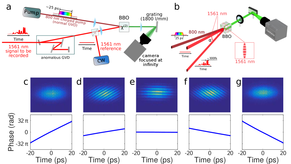
Figure 1: Heterodyne time-lens arrangement for amplitude and phase measurement of arbitrary signals. (a) Top view of the whole setup. Without the reference CW signal, the system is a time-microscope, which produces a “spatial replica” of the signal power evolution (at $\lambda_{S}\sim 1560$ nm) onto the horizontal axis of the camera (the replica has 529 nm wavelength). The noncolinear Sum Frequency Generation (SFG) between the optical field at $\lambda_{S}$ and a pump chirped pulse at $\lambda_{P}\sim 800$ nm in the BBO crystal plays the role of a “time-lens” for the $\approx$1560 nm signals (see text). Interference with the reference CW local oscillator (at $\lambda_{R}$ near $\lambda_{S}$) adds interference fringes along the vertical direction of the camera, which are used to retrieve the phase information. In the crystal, all the beams are elliptic with horizontal and vertical diameters $\sim 50\mu$m and $\sim 500\mu$m respectively. Note that all optical paths are horizontal, except the CW local oscillator signal [which enters the BBO crystal with a small angle $\alpha\sim 10$ mrad with respect to the horizontal plane, as shown in (b)]. The sub-system composed by the grating and the sCMOS camera forms a single-shot Optical Spectrum Analyzer (OSA) for the 529 nm SFG output. (c-g) Raw images and retrieved phase evolutions obtained when the signal comes from a monochromatic source with various wavelengths: $\lambda_{S}=1555.37$ nm (c), $\lambda_{S}=1559.37$ nm (d), $\lambda_{S}=1561.37$ nm (e), $\lambda_{S}=1563.37$ nm (f) and $\lambda_{S}=1567.37$ nm (g). In all case the wavelentgh of the reference is $\lambda_{R}=1561.37$ nm. For clarity, transport optics and filtering elements at BBO output have been omitted, see Sec Methods.

Our experimental setup for the measurement of phase and amplitude is displayed Figure 1.(a) and a detailed 3D enlarged view of the heterodyne time lens is plotted in Fig. 1.(b).

The time lens (i.e. the temporal quadratic phase Kolner:89 ) is provided by noncolinear Sum Frequency Generation (SFG) inside a $\chi^{(2)}$ BBO crystal between the signal field at $\lambda_{S}\sim 1560$ nm and a chirped pump pulse at $\lambda_{P}\sim 800$ nm. Measurement of the optical phase is achieved from an heterodyne setup based on the beating of the signal beam with a reference single-frequency laser emitting at a fixed wavelength $\lambda_{R}=1561$ nm. The reference beam reaches the BBO crystal by making a small vertical angle $\alpha\sim 10$ mrad with respect to the incidence plane that contains the pump beam and the signal beam. This produces an interference pattern at $\lambda\sim 1561$ nm that is copied at $\lambda_{vis}\sim 529$ nm by the process of SFG.

The spectrum of the light generated at $\lambda_{vis}$ is imaged onto the horizontal axis of the camera by using a simple diffraction grating. In the horizontal direction, the device is similar in its principle to the time microscope reported in Suret:16 where time is encoded into space : the horizontal position on the camera corresponds to the temporal evolution. Note that the horizontal (time) axis was calibrated from annex experiments involving double pulses (see Sec. Methods).

In the vertical direction, the position of the fringes of interference (i.e. for example the position of the maxima of the interference pattern) is directly proportionnal to the relative phase between the signal under investigation and the monochromatic reference field (see Sec. Methods). As a consequence, it is straightforward to extract the phase information from the pattern recorded in single shot by the sCMOS camera : the horizontal change in the vertical position of the fringes of interferences directly provides the ultrafast evolution of the phase of the signal. Our heterodyne time microscope (HTM) provides single-shot snapshots of the phase and the amplitude of the signal over time windows having a width around $40$ ps. Those single-shot recordings are performed synchronously with the pump laser, at 1 KHz repetition rate (see Sec. Methods).

.2 Tests using a continuous-wave source

In order to test our HTM and to illustrate its operating principle, we first examine the phase evolution $\phi_{S}(t)$ of a monochromatic signal having a wavelength $\lambda_{S}$ that can be tuned over some wavelength range (see Sec. Methods). The beating pattern observed on the camera is plotted in Figs. 1.(c-g) for five different values of $\lambda_{S}$. Note that the wavelength $\lambda_{R}$ of the reference laser is kept fixed. One immediatly sees that the fringes are straight lines whose slope depends on the pulsation difference $\delta\omega$ between the pulsation of the signal light and the one of the reference source. The phase $\phi_{R}$ of the reference laser can be considered as constant over each $\sim 40$ ps-long temporal window of measurement (see Sec. Methods). The relative phase $\phi(t)=\phi_{S}(t)-\phi_{R}$ is simply determined by using a procedure similar to the one described in Kreis:86 for each value of the time $t$, i.e. for each vertical line of the pattern (see Sec. Methods).

As expected we find that the phase obeys a linear time evolution $\phi(t)=\delta\omega\,t$ (see Fig. 1.(e-g)). In the experiments reported in Figs. 1.(c-g), instantaneous frequencies as large as $\delta\omega=\pm 0.8$ THz have been observed.

.3 Application to the analysis of a partially coherent light source

We now demonstrate how our device can be used to investigate phase and amplitude fluctuations of random light. Contrary to the previous situation where the signal was monochromatic, the time microscope must now be carefully set in a situation where the distance between the object under investigation and the objective lens is adjusted in such a way that a well-defined image is observed on the camera. This is achieved by carefully tuning the dispersion experienced by the random signal light by the use of a Treacy grating compressor (see Fig. 1.(a), Sec. Methods and  Kolner:89 ; Bennett:99 ; Foster:08 ; Suret:16 ).

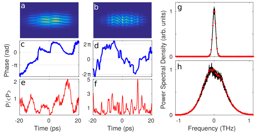
Figure 2: Phase, amplitude and spectrum of partially coherent waves (ASE). (a) and (b), Typical raw images recorded by the sCmos camera of the HTM. (c) and (d) phase retrieved from the pattern. (e) and (f) optical power normalized to the average power. Note that on fig a and b, the signal is not divided by the averaged envelop; on the contrary on the Figs. e and f the signal is divided by the average power ($P/\langle P\rangle$). The spectral width is $\Delta\nu=0.1$ THz for (a), (c), (e) and $\Delta\nu=1.$ THz for (b), (d), (f). (g) and (h) : optical spectra corresponding to $\Delta\nu=0.1$ THz and $\Delta\nu=1.$ THz respectively. Red crosses represent the spectrum computed from the averaged Fourier transform of the envelop of the electric field recorded with the HTM. Comparison with the spectrum recorded with an OSA (black line).

We first investigate the partially coherent waves emitted by an ASE light source at a wavelength $\lambda\sim 1561$ nm (see Sec. Methods). Using a programmable optical filter, the optical spectrum of the partially coherent light is designed to assume a Gaussian shape with a full width at half maximum $\Delta\nu$ that can be adjusted to some selected values.

Typical 2D patterns recorded in single shots by using the camera are displayed in Fig. 2.(a,b) while the retrieved phase $\phi(t)$ and the optical power fluctuations $P(t)$ are displayed in Figs. 2.(c,d) and 2.(e,f) for $\Delta\nu=0.1$ THz and $\Delta\nu=1$ THz respectively. Note that the retrieval algorithm is very simple and straightforward. For each value of $t$, the phase $\phi(t)$ is given by the position of the maxima and the optical power fluctuations $P(t)$ is simply computed from sum of along vertical lines of the 2D patterns and from the knowledge of the reference power previously recorded (see Sec. Methods).

As it can be expected, both the phase and of the power of the ASE light randomly fluctuate over time scales of the order of $1/\Delta\nu\sim 10$ps [Fig. 2.(c,e)] and $1/\Delta\nu\sim 1$ps [Fig. 2.(d,f)]. From additionnal experiments with pulsed laser, the temporal resolution of our heterodyne time microscope is found to be around $200$ fs.

Furthermore, a stringent test of the HTM can also be performed by comparing the optical spectrum deduced from the data, with the optical spectrum recorded independently using an optical spectrum analyzer. For each frame (recorded every ms), we compute the Fourier Transform $\widetilde{A(\omega)}$ of the complex envelop $A(t)=\sqrt{P(t)}\,e^{i\phi(t)}$ of the electric field. $P(t)$ and $\phi(t)$ represent the power and the phase of the ASE light measured by our HTM respectively. Secondly, the mean Fourier power spectrum $\langle\widetilde{|A(\omega)|^{2}}\rangle$ of the partially coherent light is computed from an average ensemble that is made over 5$\times 10^{4}$ frames. The spectral power densities computed with this procedure for $\Delta\nu=0.1$THz and $\Delta\nu=0.1$THz are plotted in red crosses on the Figs. 2.(g) and 2.(h) respectively. In both cases, the spectral power density of the ASE light separately recorded with an optical spectrum analyser (OSA) is plotted in black lines. The agreement between the spectra computed from the data recorded by the HTM and the spectra recorded with the OSA is remarkably good. These experiments with ASE light demonstrate that our HTM is indeed able to perform the accurate single-shot simultaneous measurement of phase and power of partially coherent waves fluctuating over subpicosecond time scales.

.4 Application to nonlinear random waves : optical rogue waves and Peregrine soliton in integrable turbulence

Now, we use the specific abilities of our HTM to investigate complex spatio temporal structures that emerge from nonlinear propagation of partially coherent waves inside optical fibers. For the sake of simplicity, we restrict our study to the framework of the so-called integrable turbulence Agafontsev:15 ; Walczak:15 ; SotoCrespo:16 ; Suret:16 ; Randoux:17 . This field of research, first introduced by Zakharov, deals with statistical properties of wave systems that are described by integrable equations such as the one-dimensional nonlinear Schrödinger equation (1D-NLSE) Zakharov:09 .

First, for the sake of comparison with the experiments, we perform numerical simulations of 1D-NLSE in the context of integrable turbulence (see Fig. 3). The initial conditions used in numerical simulations have the same spectral and statistical properties as the ASE light previously considered [Fig. 2.a)]. The parameters used in numerical simulations correspond to the experiments that are described below (see Sec. Methods). It is known that the emergence of rogue waves that are shown in Fig. 3.a) are responsible for deviations from the initial gaussian statistics Walczak:15 ; Suret:16 ; SotoCrespo:16 . Fig. (3.b) show typical power and phase dynamics computed after the nonlinear propagation. Up to now, it was not possible to observe this ultrafast dynamics of the phase of optical rogue waves.

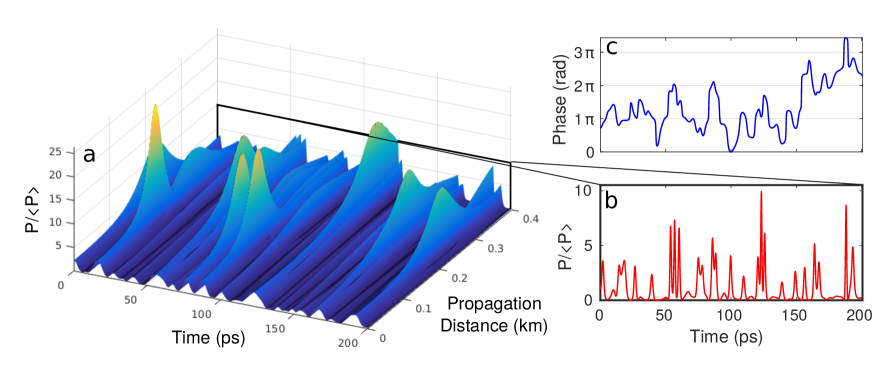
Figure 3: Numerical simulations of 1D-NLSE (a) Spatiotemporal evolution of partially coherent waves in a 400 m-long polarization maintaing fibre (PMF). The initial condition have the same spectral and statistical properties as those of the ASE light used in the experiments [See Fig. 2.a]. The parameters correspond to those of the experiments [see Fig. 4]. (b) optical power and (c) phase of partially coherent waves after the nonlinear propagation.

In order to investigate experimentally this complex phase and amplitude dynamics, we have launched partially coherent waves emitted by the ASE light source (see above and Sec. Methods) into $100$ m- or $400$ m-long Polarization Maintaining Fibres (PMF) at a wavelength falling in the anomalous (focusing) dispersion regime. The average power of the ASE light in the PMF is $\langle P\rangle\simeq 2.6$W. Fig. 4 represents the typical time evolutions of phase and amplitude that are observed at the output of the PMF by using our HTM. As mentioned above and already reported in Walczak:15 ; Suret:16 , the optical power fluctuations exhibits extreme events (RWs) having large amplitude with short time scale ($\sim 500$ fs). Remarkably, the dynamics of the phase and of the amplitude exhibit the same qualitative features in numerical simulations [Fig. 3.b] and in experiments [Fig. 4].

Single-shot recording of the phase is crucial for testing theoretical predictions of nonlinear statistical optics. This requirement is particularly stringent for unambiguous conclusions about the nature of coherent structures emerging from nonlinear random waves. As an example of the strength of our new technique, we study here the scenario implying the local formation of the Peregrine soliton (PS) that has been proposed to explain the emergence of heavy-tailed statistics Bertola:13 ; Suret:16 ; Tikan:17 .

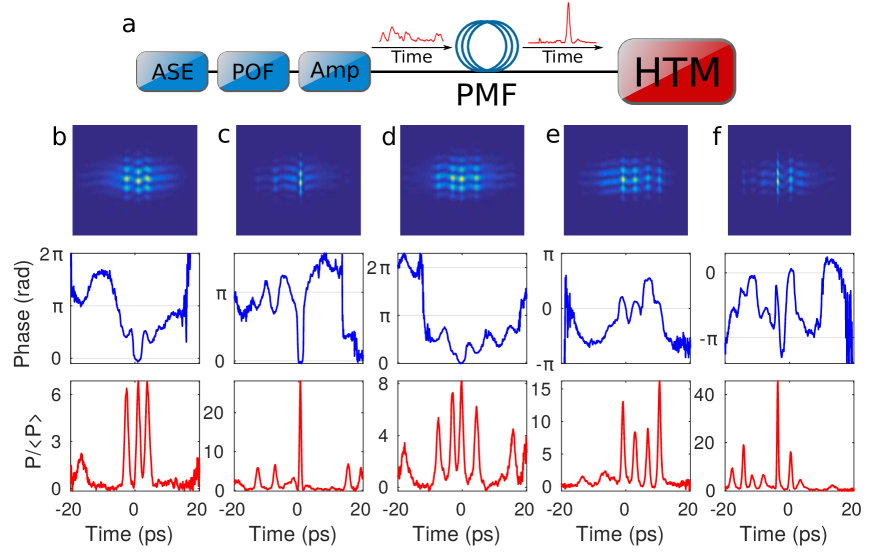
Figure 4: Experiments on nonlinear random waves (a) Experimental setup. ASE: Erbium fiber broadband Amplified Spontaneous Emission source. POF: Programmable Optical Filter to tailor the optical spectrum of the initial condition. AMP: Erbium-doped fiber Amplifier. PMF: 400 m- ong Polarization Maintaining Fibre. HTM: Heterodyne Time Microscope of Fig. 1. (b-f) Typical raw images (top) retreived phase (middle) and optical power (bottom) of partially coherent waves after nonlinear propagation in a 400m-long PMF. Note that (c) display a structure similar to the Peregrine Soliton. The initial spectral width of partially coherent waves is $\Delta\nu=0.1$THz. The Average Optical power launched into the PMF is $\langle P\rangle=2.6$W.

The temporal evolution of the power and of the phase plotted in Fig. 4.(b) shows typical structures that looks very much like the PS. Another similar structure is plotted in green line in Figs. 5.(c,d) together with plots made from the analytical formula characterizing the PS (black dashed line, see Kibler:10 ). The local intensity and phase profiles experimentally measured coincide well with those typifying the PS. In particular, one observes the characteristic $\pi$ phase jump at times where the optical power falls to zero. This observation confirms the conclusion of previous studies that the PS represents a coherent structure of special importance in the context of integrable turbulence Suret:16 ; Narhi:16 . However, by providing temporal signatures of both the phase and power profiles, our experiments definitively demonstrate that the PS can locally emerge from nonlinear random waves. This result deserves to be connected with some theoretical and experimental results which have shown that the PS is the coherent structure that is produced from the regularization of gradient catastrophes occurring in deterministic (not random) strongly nonlinear regime Bertola:13 ; Tikan:17 .

The knowledge of the phase and of the amplitude of the experimental field now opens the way to a full comparison between experiments and theory. In particular, as previously proposed in the context of experiments involving short pulses propagating in optical fibres Tsang:03 and of 2D experiments in photorefractive crystals Barsi:09 , we can perform nonlinear digital holography. The idea is to use phase and amplitude profiles measured in the experiments as initial conditions in numerical simulations of 1D-NLSE. Numerical simulations can be performed either in the backward (reverse) direction or in the forward direction (for longer propagation than in the experiments). This technique provides the spatio-temporal dynamics inside the optical fibre.

We first use experimental data recorded at the output of the $100$ m-long PMF (green lines in Figs. 5.(a,b,c,d)) as initial condition in our numerical simulations. We have integrated numerically the 1D-NLSE from $z=100$ m to $z=0$  m and from $z=100$ m to $z=200$m. The spatiotemporal evolution of the phase and amplitude obtained from numerical simulation are shown in Figs. 5.(a,b). The power and phase profiles computed from the 1D-NLSE at $z=0$ m [see red line in Fig. 5.(e,f)] reveals a good qualitative agreement with time fluctuations of the partially coherent waves launched inside the PMF and recorded with the HTM [see green line in Fig. 5.(k,i)]. In particular, the field computed at $z=0$ m exhibits fluctuations having the expected time scale ($\sim 10$ ps). The numerical integration of the 1D-NLSE between $z=100$ m and $z=200$m shows that the PS-like structure observed in our experiment would split into two sub-pulses if nonlinear propagation was prolongated over another $100$-m long PMF.

Now, the phase and amplitude profiles that have been measured for the ASE light [green line in Fig. 5.(k,i)] are used as initial conditions for the numerical integration of the 1D-NLSE between $z=0$ m to $z=200$m [see Figs. 5.(g,h)]. Numerical simulations reveals the growth of a PS-like structure that splits into two separate pulses after $z\sim 100$ m. Note that this spatio-temporal features are very similar to those typifying nonlinear propagation of the so-called N-solitons Yang ; Agrawal but here, it is found in the context of the propagation of partially coherent waves.

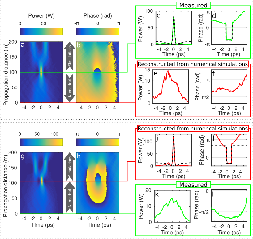
Figure 5: Nonlinear Holography : Numerical simulations of 1D-NLSE from experimental data. Top (a-f): Numerical simulation using as initial condition (green line on (a) and (b)) the experimental data recorded at the output of the 100 m PMF. Simulations are made forward (from 100 m to 200 m) and backward (from 100 m to 0 m). Spatiotemporal evolution of the power (a) and phase (b). The green inset represent plots versus time of the power (c) and phase (d) of the experimental data used as initial condition. The red inset represent plots versus time of the power (e) and phase (f) obtain after numerical simulation of the backward propagation at 0 m (red line on (a) and (b)). Dashed line: Analytical solution of the Peregrine Soliton. Bottom (g-l): same as (a-f) but the numerical simulation is made forward (from 0 m to 200 m). The green inset: initial experimental condition. Red inset: numerical result at 100 m.

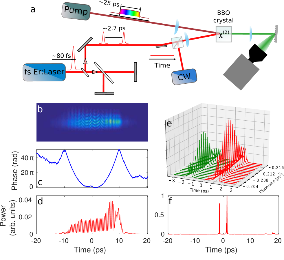
Figure 6: Digital time-holography setup (SEAHORSE), and test data. The setup displayed in (a) is similar to the one of Figure 1, except that no dispersion is induced on the signal path. In this test, we use a signal that is composed of two successive pulses with known delay. (b) Raw single-shot camera image, (c) and (d) corresponding evolutions of the phase and power (see text for their precise meanings). (f) input signal retrieved from (c,d) using a digital holography algorithm (see text). (e) signal shapes versus digital focus adjustment.

.5 Extension to high-resolution digital temporal holography

We demonstrate now that a simpler version of our heterodyne time microscope can be used to measure ultrafast dynamics of optical fields in single shot. A spatial hologram is obtained by superposition of a reference light wave and of the light coming from an object. It contains all the phase and amplitude information characterizing the object under study. In digital holography, it is possible to recompose numerically the object by applying an appropriate paraxial diffraction operator to the measured hologram  Schnars . Transposing this idea from the spatial domain to the temporal domain, we have removed the Treacy compressor from the initial setup. Thus, our device is now conceptually equivalent to a digital temporal holography device and we call it SEAHORSE (Spatial Encoding Arrangement with Hologram Observation for Recording in Single shot the Electric field).

The 2D pattern recorded with the camera is the temporal anolog to a spatial hologram contains phase and amplitude information of the initial field. As in digital (spatial) holography Schnars , we can numerically retrieve the input signal by simply computing the propagation of the recorded electric field (here by applying an adequate dispersion $\beta$, see Sec. Methods).

From the theoretical point of view, in the SEAHORSE the value of $\beta$ has to be exactly opposite to the dispersion experienced by the chirped pulse at 800 nm.

We have recorded the hologram corresponding to two 80 fs-pulses separated by $\sim 2.7$ ps (see Sec. Methods). As the spectrum of the two pulses is extremely broad ($\sim 15$THz), the 2D hologram, [Fig. 5.(b)] and the corresponding evolution of the intensity [Fig. 5.(c)] and of the phase [Fig. 5.(d)] are rather complex. However, using a GVD coefficient $\beta=-0.22$ ps² that exactly corresponds to the dispersion previously induced by the Treacy compressor, the numerical propagation of the field leads to two extremely short peaks that are separated by $2.76$ ps. Remarkably, the pulse width is $\approx 80$ fs that correspond to the the distance between two pixels of the camera. This value can be considered as representing the temporal resolution of our temporal digital holograpy device.

We want to point out that the effective resolution of the SEAHORSE ($<100$fs) is better than the resolution of the HTM. In the case of the time microscope, the resolution is limited by the aberrations due to third order dispersion of the Treacy compressor Backus:98 . The minimum temporal width that is observable with our HTM depends on the signal spectral width (as expected from aberration studies Bennett:00 ) and is around $200$ fs. SEAHORSE is somehow simpler than the usual time lens devices because the first dispersive element is not needed. Moreover SEAHORSE holographic reconstruction appears as a promising way to improve the resolution of time-lenses, by strongly reducing the aberrations, as shown here, or – potentially – even manage the aberrations a posteriori.

Discussion

In this Article, we have demonstrated two novel and complementary techniques that allow the single-shot recording of amplitude and phase of irregular waves with a high temporal resolution ($\sim 80$fs) over a long time window ($\sim 40$ ps). The key point is a completely new combination of an heterodyne technique Broaddus:10 ; Dorrer:06 and of the so-called time lens strategy that provide large temporal windows Kolner:89 ; Suret:16 ; Narhi:16

We believe that our heterodyne time lens and time holography devices will represent complementary tools to single shot versions of fast-detection devices such as FROG Trebino or SPIDER Dorrer:99 , suitable for the measurement of complex and non reproductible optical signals. The comparison between techniques introduced in this paper and already-existing single shot phase and amplitude measurement devices (e.g. time stretch Herink:17 ; Mahjoubfar:17 , XFROG Trebino ; Wong:14 , SEA-SPIDER Kosik:05 ; Wyatt:06 , SEA-TADPOLE bowlan2006crossed or STARFISH alonso2010spatiotemporal ) represents a complex question that is out of the scope of the present paper and that deserves further analysis.

We believe that the combination of large temporal window together with subpicosecond resolution represents one of the key-advantages of the setups presented in this Article. Moreover, our HTM and our time holography system do not require iterative or complex algorithm.

From the fundamental point of view, our HTM has unveiled the special evolution of the phase (and amplitude) of rogue waves in integrable turbulence, and in particular their compatibility with the expected PS Kibler:10 ; Bertola:13 ; Dudley:14 ; Toenger:15 . Our results open the way to novel and fundamental investigations of nonlinear propagation of random waves, of the emergence of optical rogue waves Solli:07 ; Akhmediev:09 ; Akhmediev:09b ; Mussot:09 ; Suret:16 ; Narhi:16 and more generally of nonlinear statistical optics Picozzi:14 .

Methods

Heterodyne time microscope

For the single-shot acquisition of phase and amplitude of sub-picosecond optical fields, heterodyne technique is implemented in an upconversion time-microscope composed  Bennett:99 of a time lens and of a single shot spectrometer very similar to the one described in Ref. Suret:16 . The heterodyne time microscope encodes the temporal change of an interference pattern onto the spectrum of a chirped pulse. The fringe pattern is imaged onto the vertical axis of a sCMOS camera and the spectrum is imaged on the horizontal axis of the camera using a 1800 lines/mm grating. The 2D pattern is recorded in single shot with $512\times 100$ pixels at the repetition rate of the $800$ nm pump laser ($1$ kHz).

We use an upconversion time-lens as in Ref. Kolner:89 (see Fig. 1). A 1 mm-long BBO crystal has cut for noncollinear type-I SFG is pumped by a 800 nm chirped pulses that are provided by an amplified Titanium-Sapphire laser (Spitfire from Spectra Physics). The laser emits 2 mJ, 40 fs pulses with a spectral bandwidth of about 25 nm) at 1 kHz repetition rate, and only 20 $\mu$J are typically used here. For inducing the required normal dispersion on the 800 nm pulses we simply adjust the amplifier’s output compressor dispersion. The dispersion was fixed to $0.21\leavevmode\nobreak\$ps², leading to chirped pulses of duration of about $25\leavevmode\nobreak\$ps.

Before being focused inside the BBO crystal, the 1560 nm signal under investigation experiences anomalous dispersion in a classic Treacy grating compressor (see Fig. 1). The 1560 nm grating compressor is made with two 600 lines/mm gratings, operated at an angle of incidence of 49 degrees, and whose planes are separated by 38.5 mm. Then, it is combined with a single-frequency reference beam at 1561 nm by using a non polarizing cube. The single-frequency reference beam is emitted by a tunable laser source having a narrow linewidth of $\sim 300$ kHz (APEX AP3350A). The coherence time scale of the reference source ($\sim 3\mu$s) is much higher than the temporal windows of recording ($\sim 40$ ps) so that the phase of the reference can be considered as being constant over each observation window. The reference light is amplified by using an Erbium-doped fibre amplifier (Keopsys) to a power of a few Watts.

The 800 nm beam, the reference beam and the signal beam are designed to assume a transverse elliptic shape by using cylindrical lenses. The horizontal waist diameter of the three beams is typically $50\,\mu$m. The vertical waist of the 1560 nm beams are typically $500\,\mu$m and the vertical waist of the 800 nm beam is typically $1$ mm. An angle $\sim 10$ mrad is adjusted in the vertical plane between the signal under investigation and the monochromatic reference in order to get several horizontal interference fringes in the observation plane.

In order to reject the 800 nm and 1560 nm radiations and to illuminate the camera with only the SFG at $529$ nm, an iris and a 40-nm bandpass filter around 531  nm (FF01 531/40-25 Semrock) is placed after the crystal. An achromatic lens with 200 mm focal length collimates the 529 nm light after the BBO crystal. The camera is a sCMOS Hamamatsu Orca flash 4.0 V3 (C13440-20CU), equiped with a 80 mm lens (Nikkor Micro 60 mm f/2.8 AF-D). The objective is focused at infinity and the waist of the SFG in the BBO crystal is imaged on the camera sensor. The camera is synchronized on the 800 nm laser pulses, and the integration time is adjusted to 1 ms, thus enabling single-shot operation of the time-microscope.

As in other time-lens systems Kolner:89 ; Bennett:99 ; Foster:08 high resolution requires proper adjustement of the dispersion produced by the 1560 nm compressor. This is conceptually analog to the focus which is required in conventional microscope, and performed by adjusting the object-objective distance. We adjust the distance between the two gratings of the Treacy compressor by minimizing the width of the image of femtosecond pulses (see Suret:16 for the details of the procedure). The best temporal resolution is achieved for a dispersion value of $\beta\simeq-0.21$ps². This value is very close to the theoretical expectation, i.e., exactly opposite to dispersion experienced by the 800nm pulse. For all results presented in this paper, the temporal resolution of the HTM is $\leavevmode\nobreak\ 200$ fs FWHM, and the field of view is around 40 ps.

Partially coherent light

The partially coherent light used in the experiments reported in Fig. 2 is generated by an Erbium fibre broadband Amplified Spontaneous Emission (ASE) source (Highwave). This broadband light is spectrally filtered (with programmable shape and linewidth) using a programmable optical filter (Waveshaper 1000S, Finisar). The filtered light is then amplified by using an Erbium-doped fibre amplifier (Keopsys). In the experiments reported in Fig. 4, the partially-coherent light obtained in this way is launched inside a single-mode polarization maintaining fibre (Fibercore HB-1550T), having either 100 m or 400 m length. The measured group velocity (second order) dispersion coefficient of the fibre is $\beta_{2}=-21$ ps²km^-1. For a given spectral width, the power of the light beam launched inside the fibre is controlled using a half-wavelength plate and a polarizing cube.

Time calibration of the HTM

Time calibration of the HTM is performed by using series of two laser pulses that are separated by a well-calibrated time delay. The pulses are emitted by a $1.5$ $\mu$m mode-locked laser (from Pritel) and have $\sim 1$ ps temporal width. Those laser pulses propagate inside a polarization maintaining fiber where they experience differential group delay depending on their state of polarization. The time separation ($5.6$ ps) between the two pulses is accurately measured from spectral interferometry. Observation of the two pulses on the sCMOS camera then permits the accurate calibration of the time axis and to measure that one camera pixel corresponds to a time duration of $78$ fs.

Data processing-Phase and power measurement

Intensity along one vertical line at the position $x$ is given by the beating between the signal beam and the reference beam. It can be presented in the form:

$$\begin{split}I&(x,y)=I_{r}(x,y)+I_{s}(x,y)\\ &+\sqrt{I_{r}(x,y)\,.\,I_{s}(x,y)}\cos[k_{y}y+\phi(x)]\end{split}$$ (1)

$I_{r}(x,y)$ represents the transverse intensity profile that is detected by the sCMOS camera in absence of the signal beam and $I_{s}(x,y)$ represents the transverse intensity profile that is detected by the sCMOS camera in absence of the reference beam. In the analysis presented in this paper, we neglect the fluctuations of the reference power. We thus compute $I_{r}(x,y)$ from additionnal experiments in which we record the SFG between the pump and the references beams (without the signal).

In the experiments, we have chosen the angle between the reference and the signal beams in order to oberve a sufficiently large number of fringes so that $\int\sqrt{I_{r}(x,y)\,.\,I_{s}(x,y)}\cos[k_{y}y+\phi(x)]\,dy\simeq 0$. For each frame, we thus simply compute the optical power $P(x)$ of the signal by using the formula :

$$P(x)=\int I(x,y)\,dy-\int I_{r}(x,y)\,dy$$ (2)

Note that here $P$ has arbitrary unit. In our study about partialy coherent waves (Figs., 2,  4 and  5) we compute the average $\langle P(x)\rangle$ from $5^{4}$ frames. We then display $P(x)/\langle P(x)\rangle$ or $[P(x)/\langle P(x)\rangle]\times P_{0}$ where $P_{0}$ is the averaged power launched inside the fiber. We remind that one pixel in $x$ corresponds to $78$ fs.

The relative phase between the signal and the reference $\phi(x)$ is simply given by the position of the maxima of the interference fringes [see Eq.(1)]. $\phi(x)$ can be easily determined by the FFT of $I(x,y)$ in the variable $y$. $\phi(x)$ is given by the phase (complex argument) of the isolated spectral peak associated with the pattern that oscillates at the frequency $k_{y}$ along the $y$ direction Kreis:86 .

Time holography

In our time holography setup, the signal under interest no longer experiences dispersion by being injected in the Treacy compressor. In a conventional microscope, this amounts to place the object under study very close to the microscope objective. With this change, we record the complex field $\psi_{H}(t)$ associated with the temporal hologram instead of the temporal image of the signal under investigation.

The time evolution of the signal under investigation $\psi(t)$ can be obtained by applying an appropriate dispersion operator in the Fourier space, i.e.

$$\tilde{\psi}(\omega)=\tilde{\psi}_{H}(\omega)\;e^{i\beta\,\omega^{2}\,/2}$$ (3)

where $\tilde{\psi}_{H}(\omega)$ and $\tilde{\psi}(\omega)$ are the Fourier transforms of $\psi_{H}(t)$ and of $\psi(t)$, respectively. From the theoretical point of view, the value of $\beta$ must be exactly equal to the group velocity dispersion (GVD) characterizing the chirped pump pulse used in the time lens.

The pair of ultra-short pulses used to demonstrate the capabilities of the time holography is produced by a femtosecond Erbium Laser (ELMO, from Menlo Systems GmbH) equipped with a Michelson interferometer. The output pulse duration at the 1553 nm central wavelength is $\leq 80$ fs and the repetition rate is 100 MHz. The energy of one pulse launched in the BBO crystal is typically $\sim 0.2$ nJ. In order to create the double pulse signal we used a Michelson interferometer with tunable optical path difference. We fixed the delay between two pulses at the value $\sim 2.7$ ps (measured with the full HTM including the Treacy compressor).

Numerical simulations of the 1D-NLSE

Numerical simulations presented in Fig. 3 and in Fig. 5 are performed by integrating the 1D-NLSE :

$$i\frac{\partial\psi}{\partial z}=-\frac{\beta_{2}}{2}\frac{\partial^{2}\psi}{\partial t^{2}}+\gamma|\psi|^{2}\psi.$$ (4)

$\psi$ represents the complex envelope of the electric field, normalized so that $|\psi|^{2}$ is the optical power. $z$ is the longitudinal coordinate measured along the fibre, and $t$ is the retarded time. $\beta_{2}=-22$ ps²km^-1 is the second-order dispersion coefficient of the fibre and $\gamma$ is the Kerr coupling coefficient. From the comparison between the optical spectra measured in the experiments and the ones computed from the numerical simulations, we estimate that the Kerr coefficient is $\gamma\sim 2.4$ W^-1km^-1. All numerical integrations are performed using splitstep pseudo-spectral methods.

In numerical simulations presented in this letter, we neglect linear losses ($\simeq 0.5$dB in the 400m-long PMF.) and stimulated Raman scattering. These approximations provide precise and quantitative agreement between experiments and numerical simulations at moderate powers ($<2$W).

Author contributions

All authors contributed to the design and the realization of the heterodyne time microscope and time holography devices. All the authors participated to the data acquisition that has been essentially performed by A.T. All authors participated to data analysis, numerical simulations and have written the manuscript.

References

- (1) Reid, D. T. et al. Roadmap on ultrafast optics. Journal of Optics 18, 093006 (2016).
- (2) Trebino, R. Frequency-resolved optical gating: the measurement of ultrashort laser pulses (Springer Science & Business Media, 2012).
- (3) Broaddus, D. H., Foster, M. A., Kuzucu, O., Koch, K. W. & Gaeta, A. L. Ultrafast, single-shot phase and amplitude measurement via a temporal imaging approach. In Conference on Lasers and Electro-Optics, CMK6 (Optical Society of America, 2010).
- (4) Bowlan, P. et al. Crossed-beam spectral interferometry: a simple, high-spectral-resolution method for completely characterizing complex ultrashort pulses in real time. Optics express 14, 11892–11900 (2006).
- (5) Alonso, B. et al. Spatiotemporal amplitude-and-phase reconstruction by fourier-transform of interference spectra of high-complex-beams. JOSA B 27, 933–940 (2010).
- (6) Rhodes, M., Steinmeyer, G. & Trebino, R. Standards for ultrashort-laser-pulse-measurement techniques and their consideration for self-referenced spectral interferometry. Applied optics 53, D1–D11 (2014).
- (7) Wetzel, B. et al. Real-time full bandwidth measurement of spectral noise in supercontinuum generation. Scientific reports 2 (2012).
- (8) Wong, T. C., Rhodes, M. & Trebino, R. Single-shot measurement of the complete temporal intensity and phase of supercontinuum. Optica 1, 119–124 (2014).
- (9) Solli, D. R., Ropers, C., Koonath, P. & Jalali, B. Optical rogue waves. Nature 450, 1054–1057 (2007).
- (10) Suret, P. et al. Single-shot observation of optical rogue waves in integrable turbulence using time microscopy. Nature communications 7 (2016).
- (11) Närhi, M. et al. Real-time measurements of spontaneous breathers and rogue wave events in optical fibre modulation instability. Nature Communications 7 (2016).
- (12) Herink, G., Kurtz, F., Jalali, B., Solli, D. R. & Ropers, C. Real-time spectral interferometry probes the internal dynamics of femtosecond soliton molecules. Science 356, 50–54 (2017).
- (13) Ryczkowski, P., Närhi, M., Billet, C., Genty, G. & Dudley, J. Real-time measurements of dissipative solitons in a mode-locked fiber laser. arXiv preprint arXiv:1706.08571 (2017).
- (14) Picozzi, A. Towards a nonequilibrium thermodynamic description of incoherent nonlinear optics. Opt. Express 15, 9063 (2007).
- (15) Turitsyna, E. G. et al. The laminar-turbulent transition in a fibre laser. Nat. Photon. 7, 783–786 (2013).
- (16) Kolner, B. H. & Nazarathy, M. Temporal imaging with a time lens. Optics letters 14, 630–632 (1989).
- (17) Foster, M. A. et al. Silicon-chip-based ultrafast optical oscilloscope. Nature 456, 81–84 (2008).
- (18) Bennett, C. & Kolner, B. Upconversion time microscope demonstrating 103 magnification of femtosecond waveforms. Optics letters 24, 783–785 (1999).
- (19) Kauffman, M., Banyai, W., Godil, A. & Bloom, D. Time-to-frequency converter for measuring picosecond optical pulses. Applied physics letters 64, 270–272 (1994).
- (20) Fridman, M. & Klein, A. Measuring the dynamics of rogue waves with unique time-lenses (conference presentation). In SPIE LASE, 100890J–100890J (International Society for Optics and Photonics, 2017).
- (21) Dorrer, C. Single-shot measurement of the electric field of optical waveforms by use of time magnification and heterodyning. Optics letters 31, 540–542 (2006).
- (22) Dorrer, C. Electric field measurement of optical waveforms (2008). URL https://www.google.com/patents/US7411683. US Patent 7,411,683.
- (23) Kosik, E. M., Radunsky, A. S., Walmsley, I. A. & Dorrer, C. Interferometric technique for measuring broadband ultrashort pulses at the sampling limit. Optics letters 30, 326–328 (2005).
- (24) Wyatt, A. S., Walmsley, I. A., Stibenz, G. & Steinmeyer, G. Sub-10 fs pulse characterization using spatially encoded arrangement for spectral phase interferometry for direct electric field reconstruction. Opt. Lett. 31, 1914–1916 (2006). URL http://ol.osa.org/abstract.cfm?URI=ol-31-12-1914.
- (25) Bertola, M. & Tovbis, A. Universality for the focusing nonlinear schrödinger equation at the gradient catastrophe point: Rational breathers and poles of the tritronquée solution to painlevé i. Communications on Pure and Applied Mathematics 66, 678–752 (2013). URL http://dx.doi.org/10.1002/cpa.21445.
- (26) Bennett, C. V. Parametric temporal imaging and aberration analysis. Ph.D. thesis, University of California (2000).
- (27) Bennett, C. V. & Kolner, B. H. Aberrations in temporal imaging. IEEE journal of quantum electronics 37, 20–32 (2001).
- (28) Salem, R., Foster, M. A. & Gaeta, A. L. Application of space–time duality to ultrahigh-speed optical signal processing. Advances in Optics and Photonics 5, 274–317 (2013).
- (29) Kreis, T. Digital holographic interference-phase measurement using the fourier-transform method. JOSA A 3, 847–855 (1986).
- (30) Agafontsev, D. & Zakharov, V. E. Integrable turbulence and formation of rogue waves. Nonlinearity 28, 2791 (2015).
- (31) Walczak, P., Randoux, S. & Suret, P. Optical rogue waves in integrable turbulence. Phys. Rev. Lett. 114, 143903 (2015).
- (32) Soto-Crespo, J. M., Devine, N. & Akhmediev, N. Integrable turbulence and rogue waves: Breathers or solitons? Phys. Rev. Lett. 116, 103901 (2016). URL http://link.aps.org/doi/10.1103/PhysRevLett.116.103901.
- (33) Randoux, S., Gustave, F., Suret, P. & El, G. Optical random riemann waves in integrable turbulence. Physical Review Letters 118, 233901 (2017).
- (34) Zakharov, V. E. Turbulence in integrable systems. Studies in Applied Mathematics 122, 219–234 (2009).
- (35) Tikan, A. et al. Universal peregrine soliton structure in nonlinear pulse compression in optical fiber. arXiv preprint arXiv:1701.08527 (2017).
- (36) Kibler, B. et al. The peregrine soliton in nonlinear fibre optics. Nature Physics 6, 790–795 (2010).
- (37) Tsang, M., Psaltis, D. & Omenetto, F. G. Reverse propagation of femtosecond pulses in optical fibers. Optics letters 28, 1873–1875 (2003).
- (38) Barsi, C., Wan, W. & Fleischer, J. W. Imaging through nonlinear media using digital holography. Nature Photonics 3, 211–215 (2009).
- (39) Yang, J. Nonlinear waves in integrable and nonintegrable systems, vol. 16 (SIAM, 2010).
- (40) Agrawal, G. P. Nonlinear Fiber optics. Optics and Photonics (Academic Press, 2001), third edition edn.
- (41) Schnars, U. & Jueptner, W. Digital holography: digital hologram recording, numerical reconstruction, and related techniques (Springer Science & Business Media, 2005).
- (42) Backus, S., Durfee III, C. G., Murnane, M. M. & Kapteyn, H. C. High power ultrafast lasers. Review of scientific instruments 69, 1207–1223 (1998).
- (43) Dorrer, C. et al. Single-shot real-time characterization of chirped-pulse amplification systems by spectral phase interferometry for direct electric-field reconstruction. Optics letters 24, 1644–1646 (1999).
- (44) Mahjoubfar, A. et al. Time stretch and its applications. Nature Photonics 11, 341–351 (2017).
- (45) Dudley, J. M., Dias, F., Erkintalo, M. & Genty, G. Instabilities, breathers and rogue waves in optics. Nat. Photon. 8, 755 (2014).
- (46) Toenger, S. et al. Emergent rogue wave structures and statistics in spontaneous modulation instability. Sci. Rep. 5 (2015).
- (47) Akhmediev, N., Ankiewicz, A. & Taki, M. Waves that appear from nowhere and disappear without a trace. Physics Letters A 373, 675 – 678 (2009).
- (48) Akhmediev, N., Soto-Crespo, J. & Ankiewicz, A. Extreme waves that appear from nowhere: On the nature of rogue waves. Physics Letters A 373, 2137 – 2145 (2009).
- (49) Mussot, A. et al. Observation of extreme temporal events in cw-pumped supercontinuum. Opt. Express 17, 17010–17015 (2009).
- (50) Picozzi, A. et al. Optical wave turbulence: Towards a unified nonequilibrium thermodynamic formulation of statistical nonlinear optics. Physics Reports 542, 1 – 132 (2014).