A Nonlinear Solution to Closed Queueing Networks for Bike Sharing Systems with Markovian Arrival Processes and under an Irreducible Path Graph

Abstract

As a favorite urban public transport mode, the bike sharing system is a large-scale and complicated system, and there exists a key requirement that a user and a bike should be matched sufficiently in time. Such matched behavior makes analysis of the bike sharing systems more difficult and challenging. To design a better bike sharing system, it is a key to analyze and compute the probabilities of the problematic (i.e., full or empty) stations. In fact, such a computation is established for some fairly complex stochastic systems. To do this, this paper considers a more general large-scale bike sharing system from two important views: (a) Bikes move in an irreducible path graph, which is related to geographical structure of the bike sharing system; and (b) Markovian arrival processes (MAPs) are applied to describe the non-Poisson and burst behavior of bike-user (abbreviated as user) arrivals, while the burstiness demonstrates that the user arrivals are time-inhomogeneous and space-heterogeneous in practice. For such a complicated bike sharing system, this paper establishes a multiclass closed queueing network by means of some virtual ideas, for example, bikes are abstracted as virtual customers; stations and roads are regarded as virtual nodes. Thus user arrivals are related to service times at station nodes; and users riding bikes on roads are viewed as service times at road nodes. Further, to deal with this multiclass closed queueing network, we provide a detailed observation practically on physical behavior of the bike sharing system in order to establish the routing matrix, which gives a nonlinear solution to compute the relative arrival rates in terms of the product-form solution to the steady-state probabilities of joint queue lengths at the virtual nodes. Based on this, we can compute the steady-state probability of problematic stations, and also deal with other interesting performance measures of the bike sharing system. We hope that the methodology and results of this paper can be applicable in the study of more general bike sharing systems through multiclass closed queueing networks.

Keywords: Bike sharing system; closed queueing network; product-form solution; irreducible path graph; problematic station; Markovian arrival process.

1 Introduction

In this paper, we propose a more general bike sharing system with Markovian arrival processes and under an irreducible path graph. Note that the bike sharing system always has some practically important factors, for example, time-inhomogeneity, geographical heterogeneity, and arrival burstiness. To analyze such a bike sharing system, we establish a multiclass closed queueing network by means of virtual customers, virtual nodes and virtual service times. Further, when studying this multiclass closed queueing network, we set up a routing matrix which gives a nonlinear solution to compute the relative arrival rates, and provide the product-form solution to the steady-state probabilities of joint queue lengths at the virtual nodes. Based on this, we can compute the steady-state probability of problematic stations, and also deal with other interesting performance measures of the bike sharing system.

During the last decades bike sharing systems have emerged as a public transport mode devoted to short trip in more than 600 major cities around the world. Bike sharing systems are regarded as a promising way to jointly reduce, such as, traffic and parking congestion, traffic noise, air pollution and greenhouse effect. Several excellent overviews and useful remarks were given by DeMaio [6], Meddin and DeMaio [23], Shu et al. [35], Labadi et al. [16] and Fishman et al. [7].

Few papers applied queueing theory and Markov processes to the study of bike sharing systems. On this research line, it is a key to compute the probability of problematic stations. However, so far there still exist some basic difficulties and challenges for computing the probability of problematic stations because computation of the steady-state probability, in the bike sharing system, needs to apply the theory of complicated or high-dimensional Markov processes. For this, readers may refer to recent literatures which are classified and listed as follows. (a) Simple queues: Leurent [17] used the M/M/1/C queue to study a vehicle-sharing system, and also analyzed performance measures of this system. Schuijbroek et al. [32] evaluated the service level by means of the transient distribution of the M/M/1/C queue, and the service level was used to establish some optimal models to discuss vehicle routing. Raviv et al. [29] and Raviv and Kolka [28] employed the transient distribution of the time-inhomogeneous M$\left(t\right)$/M$\left(t\right)$/1/C queue to compute the expected number of bike shortages at each station. (b) Closed queueing networks: Adelman [1] applied a closed queueing network to propose an internal pricing mechanism for managing a fleet of service units, and also used a nonlinear flow model to discuss the price-based policy for establishing the vehicle redistribution. George and Xia [11] used the closed queueing networks to study the vehicle rental systems, and determined the optimal number of parking spaces for each rental location. Li et al. [20] proposed a unified framework for analyzing the closed queueing networks in the study of bike sharing systems. (c) Mean-field method. Fricker et al. [8] considered a space-inhomogeneous bike-sharing system with multiple clusters, and expressed the minimal proportion of problematic stations. Fricker and Gast [9] provided a detailed analysis for a space-homogeneous bike-sharing system in terms of the M/M/1/K queue as well as some simple mean-field models, and crucially, they derived the closed-form solution to find the minimal proportion of problematic stations. Fricker and Tibi [10] studied the central limit and local limit theorems for the independent (non-identically distributed) random variables, which provide support on analysis of a generalized Jackson network with product-form solution. Further, they used the limit theorems to give an outline of stationary asymptotic analysis for the locally space-homogeneous bike-sharing systems. Li et al. [21] provided a complete picture on how to jointly use the mean-field theory, the time-inhomogeneous queues and the nonlinear birth-death processes to analyze performance measures of the bike-sharing systems. Li and Fan [19] discussed the bike sharing system under an Markovian environment by means of the mean-field computation, the time-inhomogeneous queues and the nonlinear Markov processes. (d) Markov decision processes. To discuss the bike-sharing systems, Waserhole and Jost [36, 37, 39] and Waserhole et al. [38] used the simplified closed queuing networks to establish the Markov decision models, and computed the optimal policy by means of the fluid approximation which overcame the state space explosion of multi-dimensional Markov decision processes.

There has been much key research on closed queueing networks. Readers may refer to, such as, three excellent books by Kelly [13, 14] and Serfozo [34]; multiclass customers by Baskett et al. [2], multiple closed chains by Reiser and Kobayashi [30], computational algorithms by Bruell and Balbo [4], mean-value computation by Reiser [31], sojourn time by Kelly and Pollett [15], survey for blocks by Onvural [26], and batch service by Henderson et al. [12].

Markovian arrival process (MAP) is a useful mathematical model for describing bursty traffic in, for example, communication networks, manufacturing systems, transportation networks and so forth. Readers may refer to recent publications for more details, among which are Ramaswami [27], Chapter 5 in Neuts [24], Lucantoni [22], Neuts [25], Chakravarthy [5] and Li [18].

Contributions of this paper: The main contributions of this paper are twofold: The first contribution is to propose a more general bike sharing system with Markovian arrival processes and under an irreducible path graph. Note that Markovian arrival processes, as well as the irreducible path graph indicate that burst arrival behavior and geographical structure of the bike sharing system are more general and practical. Specifically, the burstiness is to well express that the user arrivals are time-inhomogeneous and space-heterogeneous in practice. For such a bike sharing system, this paper establishes a multiclass closed queueing network by means of virtual customers, virtual nodes and virtual service times. The second contribution is to deal with such a multiclass closed queueing network with virtual customers, virtual nodes and virtual service times, and to establish a routing matrix which gives a nonlinear solution to compute the relative arrival rates in terms of the product-form solution to the steady-state probabilities of joint queue lengths at the virtual nodes. By using the product-form solution, this paper computes the steady-state probability of problematic stations, and also deals with other interesting performance measures of the bike sharing system. Therefore, the methodology and results of this paper can be applicable in the study of more general bike sharing systems by means of multiclass closed queueing networks.

Organization of this paper: The remainder of this paper is organized as follows. In Section 2, we describe a large-scale bike sharing system with Markovian arrival processes and under an irreducible path graph. In Section 3, we abstract the bike sharing system as a multiclass closed queueing network with virtual customers, virtual nodes and virtual service times. Further, we establish the routing matrix, and compute the relative arrival rate in each node, where three examples are given to express and compute the routing matrix and the relative arrival rate. In Section 4, we give a product-form solution to the steady-state probabilities of joint queue lengths at the virtual nodes, and provide a nonlinear solution to determine the $N$ undetermined constants which are related to the probability of problematic stations. Moreover, we compute the steady-state probability of problematic stations, and also analyze other performance measures of the bike sharing system. Finally, some concluding remarks are given in Section 5.

2 Model Description

In this section, we describe a more general large-scale bike sharing system, where arrivals of bike users are non-Poisson and are characterized as Markovian arrival processes (MAPs), and users riding bikes travel in an irreducible path graph which is constituted by $N$ different stations and some different directed roads.

In a large-scale bike sharing system, a user arrives at a station, rents a bike, and uses it for a while; then he returns the bike to another station, and immediately leaves this system. Based on this, we describe a more general large-scale space-heterogeneous bike sharing system, and introduce operational mechanism, system parameters and basic notation as follows:

(1) Stations: We assume that there are $N$ different stations in the bike sharing system. The $N$ stations may be different due to their geographical location and surrounding environment. We assume that every station has $C$ bikes and $K$ parking positions at the initial time $t=0$, where $1\leq C<K<\infty$, and $NC\geq K$. Note that such a condition $NC\geq K$ is to make at least a full station.

(2) Roads: Let Road $i\rightarrow j$ be a road relating Station $i$ to Station $j$. Note that Road $i\rightarrow j$ and Road $j\rightarrow i$ may be different. To express all the roads beginning from Station $i$ for $1\leq i\leq N$, we write

$$R\left(i\right)=\left\{\text{Road }i\rightarrow j:j\neq i,1\leq j\leq N\right\}.$$

Similarly, to express all roads over at Station $j$ for $1\leq j\leq N$, we write

$$\overline{R}\left(j\right)=\left\{\text{Road }i\rightarrow j:i\neq j,1\leq i\leq N\right\}.$$

It is easy to see that there are at most $N-1$ different directed roads in the set $R\left(i\right)$ or $\overline{R}\left(j\right)$. We denote by $\left|R\left(i\right)\right|$ the number of elements or roads in the set $R\left(i\right)$. Thus $\left|R\left(i\right)\right|\leq N-1$ for $1\leq i\leq N$ and $\sum\nolimits_{i=1}^{N}\left|R\left(i\right)\right|\leq N\left(N-1\right)$.

To express all the stations in the near downlink of Station $i$, we write

$$\Theta_{i}=\left\{j:\text{Road }i\rightarrow j\in R\left(i\right)\right\}.$$

Similarly, the set of all stations in the near uplink of Station $i$ is written as

$$\Delta_{i}=\left\{j:\text{Road }j\rightarrow i\in\overline{R}\left(i\right)\right\}.$$

(3) An irreducible path graph: To express the bike moving paths, it is easy to observe that the bikes dynamically move among the stations and among the roads. To record the bike dynamic positions, it is better to introduce two classes of virtual nodes: (a) station nodes; and (b) road nodes. The set of all the virtual nodes of the bike sharing system is given by

$$\Theta=\left\{\text{Station }i:1\leq i\leq N\right\}\cup\left\{\underset{i=1}{\overset{N}{\cup}}R\left(i\right)\right\}.$$

In this bike sharing system, it is easy to calculate that there are $N+\cup_{i=1}^{N}\left|R\left(i\right)\right|$ virtual nodes.

If Station $i$ has a near downstream Road $i\rightarrow j$, then we call that Node $i$ (i.e. Station $i$) can be accessible to Node $i\rightarrow j$ (i.e. Road $i\rightarrow j$), denoted as Node $i\Longrightarrow$ Node $i\rightarrow j$; otherwise Node $i$ can not be accessible to Node $i\rightarrow j$. If Station $j$ has a near upstream Road $i\rightarrow j$, then we call that Node $i\rightarrow j$ can be accessible to Node $j$, denoted as Node $i\rightarrow j\Longrightarrow$ Node $j$; otherwise Node $i\rightarrow j$ can not be accessible to Node $j$.

If there exist some virtual nodes $n_{1},n_{2},\ldots,n_{r}$ in the set $\Theta$ such that

$$\text{Node }n_{1}\Longrightarrow\text{Node }n_{2}\Longrightarrow\cdots\Longrightarrow\text{Node }n_{r},$$

then we call that there is an accessible path formed by the virtual nodes $n_{1},n_{2},$ $\ldots,n_{r}$.

If for any two virtual nodes $m_{a}$ and $m_{b}$ in the set $\Theta$, there always exist some virtual nodes $n_{1},n_{2},\ldots,n_{r}$ in the set $\Theta$ such that

$$\text{Node }m_{a}\Longrightarrow\text{Node }n_{1}\Longrightarrow\text{Node }n_{2}\Longrightarrow\cdots\Longrightarrow\text{Node }n_{r}\Longrightarrow\text{Node }m_{b},$$

then we call that the path graph of the bike sharing system is irreducible.

In this paper, we assume that the bike sharing system exists an irreducible path graph. In this case, we call that the bike sharing system is path irreducible. Note that this irreducibility is guaranteed through setting up an appropriate road construction with $R\left(i\right)$ for $1\leq i\leq N$. In general, such a road construction is not unique in order to guarantee the irreducible path graph.

(4) Markovian arrival processes: Arrivals of outside bike users at Station $i$ are a Markovian arrival process (MAP) of irreducible matrix descriptor $\left(\mathbf{C}_{i},\mathbf{D}_{i}\right)$ of size $m$, denoted as MAP$\left(\mathbf{C}_{i},\mathbf{D}_{i}\right)$, where

$$\mathbf{C}_{i}=\left(\begin{array}[c]{cccc}c_{1,1}^{\left(i\right)}&c_{1,2}^{\left(i\right)}&\cdots&c_{1,m}^{\left(i\right)}\\ c_{2,1}^{\left(i\right)}&c_{2,2}^{\left(i\right)}&\cdots&c_{2,m}^{\left(i\right)}\\ \vdots&\vdots&\ddots&\vdots\\ c_{m,1}^{\left(i\right)}&c_{m,2}^{\left(i\right)}&\cdots&c_{m,m}^{\left(i\right)}\end{array}\right)$$

and

$$\mathbf{D}_{i}=\left(\begin{array}[c]{cccc}d_{1,1}^{\left(i\right)}&d_{1,2}^{\left(i\right)}&\cdots&d_{1,m}^{\left(i\right)}\\ d_{2,1}^{\left(i\right)}&d_{2,2}^{\left(i\right)}&\cdots&d_{2,m}^{\left(i\right)}\\ \vdots&\vdots&\ddots&\vdots\\ d_{m,1}^{\left(i\right)}&d_{m,2}^{\left(i\right)}&\cdots&d_{m,m}^{\left(i\right)}\end{array}\right).$$

Let $c_{k,l}^{\left(i\right)}\geq 0$ with $l\neq k$, $d_{r,s}^{\left(i\right)}\geq 0$, $c_{k,k}^{\left(i\right)}=-\left(\sum\limits_{l\neq k}^{m}c_{k,l}^{\left(i\right)}+\sum\limits_{r=1}^{m}d_{k,r}^{\left(i\right)}\right)$, and hence $\left(\mathbf{C}_{i}+\mathbf{D}_{i}\right)e=0$. We assume that Markov chain $\mathbf{C}_{i}+\mathbf{D}_{i}$ is irreducible, finite-state and aperiodic, hence it is positive-recurrent due to the finite state space. Further, in the Markov chain $\mathbf{C}_{i}+\mathbf{D}_{i}$ there exists the unique stationary probability vector $\widetilde{\theta}^{\left(i\right)}=\left(\theta_{1}^{\left(i\right)},\theta_{2}^{\left(i\right)},\cdots,\theta_{m}^{\left(i\right)}\right)$ for $1\leq i\leq N$, that is, the vector $\widetilde{\theta}^{\left(i\right)}$ is the unique solution to the system of linear equations $\widetilde{\theta}^{\left(i\right)}\left(\mathbf{C}_{i}+\mathbf{D}_{i}\right)=0$ and $\widetilde{\theta}^{\left(i\right)}e=1$. In this case, the stationary average arrival rate of the MAP$\left(\mathbf{C}_{i}+\mathbf{D}_{i}\right)$ is $\lambda_{i}=\widetilde{\theta}^{\left(i\right)}D^{\left(i\right)}e$. Specifically, we write that $\overrightarrow{\lambda}_{i}=\left(\lambda_{i}^{\left(1\right)},\lambda_{i}^{\left(2\right)},\cdots,\lambda_{i}^{\left(m\right)}\right)=\widetilde{\theta}^{\left(i\right)}\mathbf{D}_{i}$ for $1\leq i\leq N$.

(5) The first riding-bike time: An outside bike user arrives at the $i$th station to rent a bike. If there is no bike in the $i$th station (i.e., the $i$th station is empty), then the user immediately leaves this bike sharing system. If there is at least one available bike at the $i$th station, then the user rents a bike and goes to Road $i\rightarrow j$ for $j\neq i$ with probability $p_{i,j}$ for $\sum_{j\in\Theta_{i}}p_{i,j}=1$, and his riding-bike time on Road $i\rightarrow j$ is an exponential random variable with riding-bike rate $\mu_{i,j}>0$.

(6) The bike return times:

Notice that for any user, his first bike return process may be different from those retrial processes with successively returning the bike to one station for at least twice due to his pasted arrivals at the full stations. In this situation, his road selection as well as his riding-bike time in the first process may be different from those in any retrial return process.

The first return – When the user completes his short trip on Road $i\rightarrow j$, he needs to return his bike to the $j$th station. If there is at least one available parking position (i.e., a vacant docker), then the user directly returns the bike to the $j$th station, and immediately leaves this bike sharing systems.

The second return – If no parking position is available at the $j$th station, then the user has to ride the bike to the $l_{1}$th station with probability $\alpha_{j,l_{1}}$ for $l_{1}\neq j$ and $\sum_{l_{1}\in\Theta_{j}}\alpha_{j,l_{1}}=1$; and his future riding-bike time on Road $j\rightarrow l_{1}$ is also an exponential random variable with riding-bike rate $\xi_{j,l_{1}}>0$. If there is at least one available parking position, then the user directly returns his bike to the $l_{1}$th station, and immediately leaves this bike sharing system.

The ($k+1$)st return for $k\geq 2$ – We assume that this bike has not been returned at any station yet through $k$ consecutive returns. In this case, the user has to try his ($k+1$)st lucky return. Notice that the user goes to the $l_{k}$th station from the $l_{k-1}$th full station with probability $\alpha_{l_{k-1},l_{k}}$ for $l_{k}\neq l_{k-1}$ and $\sum_{l_{k}\in\Theta_{l_{k-1}}}\alpha_{l_{k-1},l_{k}}=1$; and his riding-bike time on Road $l_{k-1}\rightarrow l_{k}$ is an exponential random variable with riding-bike rate $\xi_{l_{k-1},l_{k}}>0$. If there is at least one available parking position, then the user directly returns his bike to the $l_{k}$th station, and immediately leaves this bike sharing system; otherwise he has to continuously ride his bike in order to try to return the bike to another station again.

We further assume that the returning-bike process is persistent in the sense that the user must find a station with an empty position to return his bike because the bike is a public property.

It is seen from the above description that the parameters: $p_{i,j}$ and $\mu_{i,j}$, for $j\neq i$ and $1\leq i,j\leq N$, of the first return, may be different from the parameters: $\alpha_{i,j}$ and $\xi_{i,j}$, for $j\neq i$ and $1\leq i,j\leq N$, of the $k$th return for $k\geq 2$. This is due to a simple observation that the user possibly deal with more things (for example, tourism, shopping, visiting friends and so on) in the first return process, but he becomes only one return task for returning his bike to one station during the $k$ successive return processes for $k\geq 2$.

(7) The departure discipline: The user departure process has two different cases: (a) An outside user directly leaves the bike sharing system if he arrives at an empty station; and (b) if one user rents and uses a bike, and he finally returns the bike to a station, then the user completes his trip, and immediately leaves the bike sharing system.

We assume that all the above random variables are independent of each other. For such a bike sharing system, Fig. 1 provides some intuitive physical interpretation for the bike sharing system.

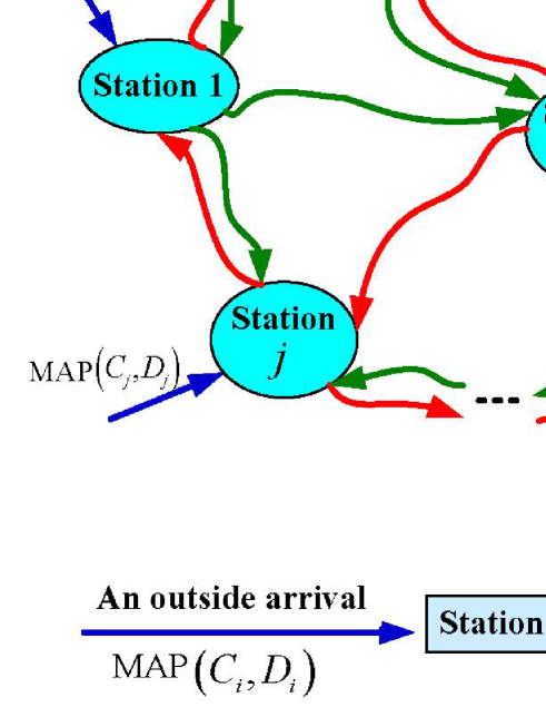
Figure 1: The physical structure of the bike sharing system

3 A Closed Queueing Network

In this section, we describe the bike sharing system as a closed queueing network according to the fact that the number of bikes in this system is fixed. To study such a closed queueing network, we need to determine the service rates, the routing matrix and the relative arrival rates in all the virtual nodes.

For the bike sharing system, we need to abstract it as a closed queueing network as follows:

(1) Virtual nodes: Although the stations and the roads have different physical attributes, such as, different functions, different geographical topologies and so forth, it is seen that here the stations and the roads are all regarded as the same abstructed nodes in a closed queueing network.

(2) Virtual customers: The bikes either at the stations or on the roads are viewed as virtual customers as follows:

A closed queueing network under virtual idea: The virtual customers are abstracted by the bikes from either the stations or the roads. In this case, the service processes are taken either from user arrivals at the station nodes or from users riding bikes on the road nodes. Since the total number of bikes in the bike sharing system is fixed as the positive integer $NC$, thus the bike sharing system can be regarded as a closed queueing network with such virtual customers, virtual nodes and virtual service times.

Two classes of virtual customers: From Assumptions (2), (5) and (6) in Section 2, it is seen that there are two different classes of virtual customers in the road nodes, where the first class of virtual customers are the bikes ridden on the roads for the first time; while the second class of virtual customers are the bikes which are successively ridden on the roads at least twice due to his arrivals at full stations.

We abstract the virtual nodes both from the stations and from the roads, and also find the virtual customers corresponding to the $NC$ bikes. This sets up a multiclass closed queueing network. To compute the steady-state probabilities of joint queue lengths in the bike sharing system, it is seen from Chapter 7 in Bolch et al. [3] that we need to determine the service rate and the relative arrival rate for each virtual node in the multiclass closed queueing network.

(a) The service rates at nodes

We discuss the service processes of the closed queueing network from two different cases: One for the station nodes, and the other for the road nodes. Fig. 2 shows how the two classes of service times are given from the multiclass closed queueing network.

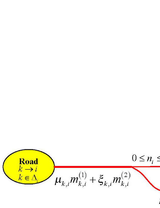
Figure 2: The queueing processes in the multiclass closed queueing network

Case one: A road node in the set $\cup_{i=1}^{N}R\left(i\right)$

The first class of virtual customers: We denote the number of virtual customers of the first class on Road $i\rightarrow l$ by $m_{i,l}^{\left(1\right)}$. The return process of bikes of the first class from Road $i\rightarrow l$ to Station $l$ for the first time is Poisson with service rate

$$a_{i,l}^{\left(1\right)}=m_{i,l}^{\left(1\right)}\mu_{i,l}.$$

The second class of virtual customers: We denote the number of virtual customers of the second class on Road $i\rightarrow l$ by $m_{i,l}^{\left(2\right)}$. The retrial return process of customers of the second class from Road $i\rightarrow j$ to Station $l$ is Poisson with service rate

$$a_{i,l}^{\left(2\right)}=m_{i,l}^{\left(2\right)}\xi_{i,l}.$$

Case two: The $N$ station nodes

Let $n_{i}$ be the number of bikes packed in Station $i$. The departure process of bikes from the $i$th station is due to those customers who rent the bikes at the $i$th station and then immediately enter one road in $R\left(i\right)$. Thus if the $i$th station is not empty, then the service process (i.e. renting bikes) is a MAP with a stationary service rate of phase $v$

$$a_{i}^{\left(v\right)}=\lambda_{i}^{\left(v\right)}\mathbf{1}_{\left\{1\leq n_{i}\leq K\right\}}\sum_{l\neq i}^{N}p_{i,l}=\lambda_{i}^{\left(v\right)}\mathbf{1}_{\left\{1\leq n_{i}\leq K\right\}},1\leq v\leq m,$$ (1)

where $\sum_{l\neq i}^{N}p_{i,l}=1$, and $\overrightarrow{\lambda}_{i}=\left(\lambda_{i}^{\left(1\right)},\lambda_{i}^{\left(2\right)},\ldots,\lambda_{i}^{\left(m\right)}\right)$ is given by the MAP $\left(C_{i},D_{i}\right)$ through $\overrightarrow{\lambda}_{i}=\widetilde{\theta}^{\left(i\right)}D_{i}$ for $1\leq i\leq N$.

(b) The relative arrival rates

For the multiclass closed queueing network, to determine the steady-state probability distribution of joint queue lengths at any virtual node, it is necessary to firstly give the relative arrival rates at the virtual nodes. To this end, we must establish the routing matrix in the first step.

Based on Chapter 7 in Bolch et al. [3], we denote by $e_{i}$ and $e_{R_{i\rightarrow j}}^{\left(r\right)}$ the relative arrival rates of the $i$th station, and of Road $i\rightarrow l$ with bikes of class $r$, respectively. We write

$$\overrightarrow{e}=\left\{\overrightarrow{e}_{i}:1\leq i\leq N\right\},$$

where

$$\overrightarrow{e}_{i}=\left\{\mathbf{e}_{i},\mathbf{e}_{R_{i\rightarrow j}}^{\left(r\right)},j\in\Theta_{i},r=1,2\right\}.$$

Note that this bike sharing system is large-scale, thus the routing matrix of the closed queueing network corresponding to the bike sharing system will be very complicated. To understand how to set up such a routing matrix, in what follows we first give three simple examples for the purpose of writing the routing matrix, using the physical structure and the routing graph of the bike sharing system. See Figures 3 to 5 for more details.

Let $Q_{i}\left(t\right)$ be the number of bikes parked at Station $i$ at time $t\geq 0$. From the exponential and MAP assumptions, it is seen that an irreducible finite state Markov chain is used to express and analyze the bike sharing system, while the Markov chain is aperiodic and positive recurrent. In this case, there exists stationary probability vector in the Marokov chain, and thus we give the limit

$$\pi_{i,K}=\underset{t\rightarrow+\infty}{\lim}P\left\{Q_{i}\left(t\right)=K\right\}.$$

Example One: We consider a simple bike sharing system with two stations, and the physical structure of the stations and roads is depicted in (a) of Fig.3. Note that there exist two classes of virtual customers in the road nodes, and the bike routing graph of the bike sharing system is depicted in (b) of Fig.3. Since there are only two stations in this bike sharing system, we have $p_{i,j}=\alpha_{i,j}=1$. Based on this, we obtain the routing matrix of order 6 as follow:

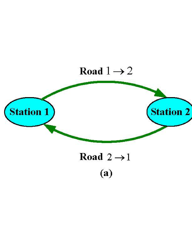
Figure 3: The physical structure (a) and the bike routing graph (b) for a two-station bike sharing system

$$P=\left(\begin{array}[c]{llllll}&1&&&&\\ &&&1-\pi_{2,K}&&\pi_{2,K}\\ &&&1-\pi_{2,K}&&\pi_{2,K}\\ &&&&1&\\ 1-\pi_{1,K}&&\pi_{1,K}&&&\\ 1-\pi_{1,K}&&\pi_{1,K}&&&\end{array}\right),$$

where all those elements that are not expressed are viewed as zeros, and $\pi_{i,K}$ is a undetermined constant, and it is also the stationary probability of the $i$th full station for $i=1,2$.

To determine the relative arrival rate at each virtual node, using the system of linear equations $\overrightarrow{e}P=\overrightarrow{e}$ and $e_{1}=1$, we obtain

$$\left\{\begin{array}[]{l}e_{1}=\left(e_{R_{2\rightarrow 1}}^{\left(1\right)}+e_{R_{2\rightarrow 1}}^{\left(2\right)}\right)\left(1-\pi_{1,K}\right),\\ e_{R_{1\rightarrow 2}}^{\left(1\right)}=e_{1},\\ e_{R_{1\rightarrow 2}}^{\left(2\right)}=\left(e_{R_{2\rightarrow 1}}^{\left(1\right)}+e_{R_{2\rightarrow 1}}^{\left(1\right)}\right)\pi_{1,K},\\ e_{2}=\left(e_{R_{1\rightarrow 2}}^{\left(1\right)}+e_{R_{1\rightarrow 2}}^{\left(2\right)}\right)\left(1-\pi_{2,K}\right),\\ e_{R_{2\rightarrow 1}}^{\left(1\right)}=e_{2},\\ e_{R_{2\rightarrow 1}}^{\left(2\right)}=\left(e_{R_{1\rightarrow 2}}^{\left(1\right)}+e_{R_{1\rightarrow 2}}^{\left(2\right)}\right)\pi_{2,K}.\end{array}\right.$$

Using $e_{1}=1$, we get

$$\left\{\begin{array}[]{l}e_{1}=e_{R_{1\rightarrow 2}}^{\left(1\right)}=1,\\ e_{R_{1\rightarrow 2}}^{\left(2\right)}=\frac{\pi_{1,K}}{1-\pi_{1,K}},\\ e_{2}=e_{R_{2\rightarrow 1}}^{\left(1\right)}=\frac{1-\pi_{2,K}}{1-\pi_{1,K}},\\ e_{R_{2\rightarrow 1}}^{\left(2\right)}=\frac{\pi_{2,K}}{1-\pi_{1,K}},\end{array}\right.$$ (2)

where the two undetermined positive constants $\pi_{1,K}$ and $\pi_{2,K}$ will be given in the next section, and they determine the relative arrival rates at the six virtual nodes.

Example Two: We consider a bike sharing system with three stations, and the physical structure of the stations and roads can be seen in (a) of Fig.4. There exist two classes of virtual customers in the road nodes, and the bike routing graph of the bike sharing system is depicted in (b) of Fig.4. It is seen from (a) of Fig.4 that $p_{1,2}=p_{2,3}=p_{3,1}=\alpha_{1,2}=\alpha_{2,3}=\alpha_{3,1}=1$. Based on this, the routing matrix of order 9 is given by

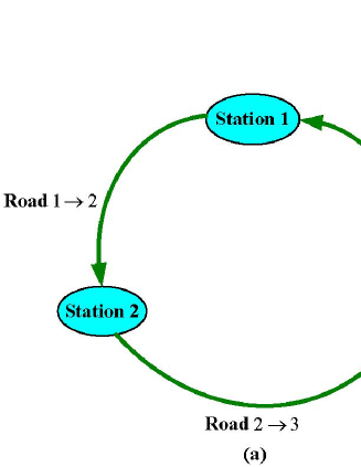
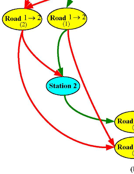
Figure 4: The physical structure (a) and the bike routing graph (b) of a three-station bike sharing system

$$\left(\begin{array}[c]{lllllllll}&1&&&&&&&\\ &&&1-\pi_{2,K}&&\pi_{2,K}&&&\\ &&&1-\pi_{2,K}&&\pi_{2,K}&&&\\ &&&&1&&&&\\ &&&&&&1-\pi_{3,K}&&\pi_{3,K}\\ &&&&&&1-\pi_{3,K}&&\pi_{3,K}\\ &&&&&&&1&\\ 1-\pi_{1,K}&&\pi_{1,K}&&&&&&\\ 1-\pi_{1,K}&&\pi_{1,K}&&&&&&\end{array}\right).$$

To determine the relative arrival rate at each virtual node, using the system of linear equations $\overrightarrow{e}P=\overrightarrow{e}$ and $e_{1}=1$, we obtain

$$\left\{\begin{array}[]{l}e_{1}=\left(e_{R_{3\rightarrow 1}}^{\left(1\right)}+e_{R_{3\rightarrow 1}}^{\left(2\right)}\right)\left(1-\pi_{1,K}\right),\\ e_{R_{1\rightarrow 2}}^{\left(1\right)}=e_{1},\\ e_{R_{1\rightarrow 2}}^{\left(2\right)}=\left(e_{R_{3\rightarrow 1}}^{\left(1\right)}+e_{R_{3\rightarrow 1}}^{\left(2\right)}\right)\pi_{1,K},\\ e_{2}=\left(e_{R_{1\rightarrow 2}}^{\left(1\right)}+e_{R_{1\rightarrow 2}}^{\left(2\right)}\right)\left(1-\pi_{2,K}\right),\\ e_{R_{2\rightarrow 3}}^{\left(1\right)}=e_{2},\\ e_{R_{2\rightarrow 3}}^{\left(2\right)}=\left(e_{R_{1\rightarrow 2}}^{\left(1\right)}+e_{R_{1\rightarrow 2}}^{\left(2\right)}\right)\pi_{2,K},\\ e_{3}=\left(e_{R_{2\rightarrow 3}}^{\left(1\right)}+e_{R_{2\rightarrow 3}}^{\left(2\right)}\right)\left(1-\pi_{3,K}\right),\\ e_{R_{3\rightarrow 1}}^{\left(1\right)}=e_{3},\\ e_{R_{3\rightarrow 1}}^{\left(2\right)}=\left(e_{R_{2\rightarrow 3}}^{\left(1\right)}+e_{R_{2\rightarrow 3}}^{\left(2\right)}\right)\pi_{3,K}.\end{array}\right.$$

Using $e_{1}=1$, we get

$$\left\{\begin{array}[]{l}e_{1}=e_{R_{1\rightarrow 2}}^{\left(1\right)}=1,\\ e_{R_{1\rightarrow 2}}^{\left(2\right)}=\frac{\pi_{1,K}}{1-\pi_{1,K}}\\ e_{2}=e_{R_{2\rightarrow 3}}^{\left(1\right)}=\frac{1-\pi_{2,K}}{1-\pi_{1,K}},\\ e_{R_{2\rightarrow 3}}^{\left(2\right)}=\frac{\pi_{2,K}}{1-\pi_{1,K}},\\ e_{3}=e_{R_{3\rightarrow 1}}^{\left(1\right)}=\frac{1-\pi_{3,K}}{1-\pi_{1,K}},\\ e_{R_{3\rightarrow 1}}^{\left(2\right)}=\frac{\pi_{3,K}}{1-\pi_{1,K}},\end{array}\right.$$ (3)

where the three undetermined positive constants $\pi_{1,K}$, $\pi_{2,K}$ and $\pi_{3,K}$ will be given in the next section, and they determine the relative arrival rates for the nine virtual nodes.

Example Three: We consider a bike sharing system with three stations, and the physical structure of the stations and roads can be seen in (a) of Fig.5. There exist two classes of virtual customers in the road nodes, and the bike routing graph of the bike sharing system is depicted in (b) of Fig.5. Based on this, we obtain the routing matrix of order 11 as follow:

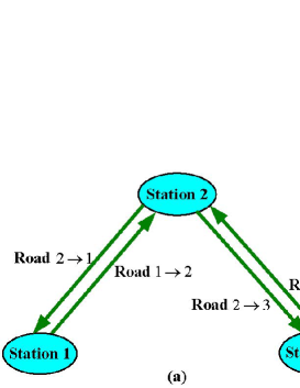
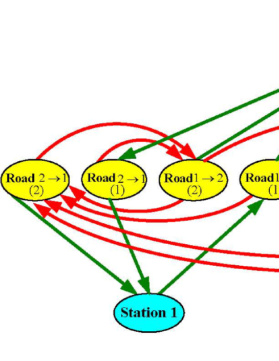
Figure 5: The physical structure (a) and the bike routing graph (b) of a three-station bike sharing system

$$\left(\begin{array}[]{ccccccccccc}&1&&&&&&&&&\\ &&&1-\pi_{2,K}&&\alpha_{2,1}\pi_{2,K}&&\alpha_{2,3}\pi_{2,K}&&&\\ &&&1-\pi_{2,K}&&\alpha_{2,1}\pi_{2,K}&&\alpha_{2,3}\pi_{2,K}&&&\\ &&&&p_{2,1}&&p_{2,3}&&&&\\ 1-\pi_{1,K}&&\pi_{1,K}&&&&&&&&\\ 1-\pi_{1,K}&&\pi_{1,K}&&&&&&&&\\ &&&&&&&&1-\pi_{3,K}&&\pi_{3,K}\\ &&&&&&&&1-\pi_{3,K}&&\pi_{3,K}\\ &&&&&&&&&1&\\ &&&1-\pi_{2,K}&&\alpha_{2,1}\pi_{2,K}&&\alpha_{2,3}\pi_{2,K}&&&\\ &&&1-\pi_{2,K}&&\alpha_{2,1}\pi_{2,K}&&\alpha_{2,3}\pi_{2,K}&&&\end{array}\right).$$

To determine the relative arrival rate at each virtual node, using the system of linear equations $\overrightarrow{e}P=\overrightarrow{e}$ and $e_{1}=1$, we obtain

$$\left\{\begin{array}[]{l}e_{1}=\left(e_{R_{2\rightarrow 1}}^{\left(1\right)}+e_{R_{2\rightarrow 1}}^{\left(2\right)}\right)\left(1-\pi_{1,K}\right),\\ e_{R_{1\rightarrow 2}}^{\left(1\right)}=e_{1},\\ e_{R_{1\rightarrow 2}}^{\left(2\right)}=\left(e_{R_{2\rightarrow 1}}^{\left(1\right)}+e_{R_{2\rightarrow 1}}^{\left(2\right)}\right)\pi_{1,K}\\ e_{2}=\left(e_{R_{1\rightarrow 2}}^{\left(1\right)}+e_{R_{1\rightarrow 2}}^{\left(2\right)}+e_{R_{3\rightarrow 2}}^{\left(1\right)}+e_{R_{3\rightarrow 2}}^{\left(2\right)}\right)\left(1-\pi_{2,K}\right),\\ e_{R_{2\rightarrow 1}}^{\left(1\right)}=p_{2,1}e_{2},\\ e_{R_{2\rightarrow 1}}^{\left(2\right)}=\left(e_{R_{1\rightarrow 2}}^{\left(1\right)}+e_{R_{1\rightarrow 2}}^{\left(2\right)}+e_{R_{3\rightarrow 2}}^{\left(1\right)}+e_{R_{3\rightarrow 2}}^{\left(2\right)}\right)\alpha_{2,1}\pi_{2,K},\\ e_{R_{2\rightarrow 3}}^{\left(1\right)}=p_{2,3}e_{2},\\ e_{R_{2\rightarrow 3}}^{\left(2\right)}=\left(e_{R_{1\rightarrow 2}}^{\left(1\right)}+e_{R_{1\rightarrow 2}}^{\left(2\right)}+e_{R_{3\rightarrow 2}}^{\left(1\right)}+e_{R_{3\rightarrow 2}}^{\left(2\right)}\right)\alpha_{2,3}\pi_{2,K},\\ e_{3}=\left(e_{R_{2\rightarrow 3}}^{\left(1\right)}+e_{R_{2\rightarrow 3}}^{\left(2\right)}\right)\left(1-\pi_{3,K}\right),\\ e_{R_{3\rightarrow 2}}^{\left(1\right)}=e_{3},\\ e_{R_{3\rightarrow 2}}^{\left(2\right)}=\left(e_{R_{2\rightarrow 3}}^{\left(1\right)}+e_{R_{2\rightarrow 3}}^{\left(2\right)}\right)\pi_{3,K}.\end{array}\right.$$ (4)

By using $e_{1}=1$, we obtain

$$\left\{\begin{array}[]{l}e_{1}=e_{R_{1\rightarrow 2}}^{\left(1\right)}=1,\\ e_{R_{1\rightarrow 2}}^{\left(2\right)}=\frac{\pi_{1,K}}{1-\pi_{1,K}}\\ e_{2}=\frac{1-\pi_{2,K}}{\left(1-\pi_{1,K}\right)\left[\left(\alpha_{2,1}-p_{2,1}\right)\pi_{2,K}+p_{2,1}\right]},\\ e_{R_{2\rightarrow 1}}^{\left(1\right)}=\frac{p_{2,1}\left(1-\pi_{2,K}\right)}{\left(1-\pi_{1,K}\right)\left[\left(\alpha_{2,1}-p_{2,1}\right)\pi_{2,K}+p_{2,1}\right]},\\ e_{R_{2\rightarrow 1}}^{\left(2\right)}=\frac{\alpha_{2,1}\pi_{2,K}}{\left(1-\pi_{1,K}\right)\left[\left(\alpha_{2,1}-p_{2,1}\right)\pi_{2,K}+p_{2,1}\right]},\\ e_{R_{2\rightarrow 3}}^{\left(1\right)}=\frac{p_{2,3}\left(1-\pi_{2,K}\right)}{\left(1-\pi_{1,K}\right)\left[\left(\alpha_{2,1}-p_{2,1}\right)\pi_{2,K}+p_{2,1}\right]},\\ e_{R_{2\rightarrow 3}}^{\left(2\right)}=\frac{\alpha_{2,3}\pi_{2,K}}{\left(1-\pi_{1,K}\right)\left[\left(\alpha_{2,1}-p_{2,1}\right)\pi_{2,K}+p_{2,1}\right]},\\ e_{3}=e_{R_{3\rightarrow 1}}^{\left(1\right)}=\frac{\left(1-\pi_{3,K}\right)\left[\left(\alpha_{2,3}-p_{2,3}\right)\pi_{2,K}+p_{2,3}\right]}{\left(1-\pi_{1,K}\right)\left[\left(\alpha_{2,1}-p_{2,1}\right)\pi_{2,K}+p_{2,1}\right]},\\ e_{R_{3\rightarrow 1}}^{\left(2\right)}=\frac{\pi_{3,K}\left[\left(\alpha_{2,3}-p_{2,3}\right)\pi_{2,K}+p_{2,3}\right]}{\left(1-\pi_{1,K}\right)\left[\left(\alpha_{2,1}-p_{2,1}\right)\pi_{2,K}+p_{2,1}\right]}.\end{array}\right.$$

The routing matrices for more general case

Observing the three examples, it may be easy and convenient to write a routing matrix for a more general bike sharing system. Note that Example Three provides more intuitive understanding on how to write those elements of the routing matrix, thus for a more general bike sharing system we establish the routing matrix $\mathbf{P}=\left(p_{\widetilde{i},\widetilde{j}}\right)$ as follow:

$$p_{\widetilde{i},\widetilde{j}}=\left\{\begin{array}[]{ll}p_{i,j},&\text{if }\widetilde{i}=\text{Station }i,\widetilde{j}=\text{Road }i\rightarrow j\\ 1-\pi_{j,K},&\text{if }\widetilde{i}=\text{Road }i\rightarrow j,\widetilde{j}=\text{Station }j\\ \sum\limits_{l\in\Theta_{i}\&l\in\Delta_{j}}\alpha_{l,j}\pi_{l,K},&\text{if }n_{l}=K,\widetilde{i}=\text{Road }i\rightarrow l,\widetilde{j}=\text{Road }l\rightarrow j\\ 0.&\text{otherwise}\end{array}\right.$$

Theorem 1

The routing matrix $\mathbf{P}$ of finite size is irreducible and stochastic, and there exists the unique positive solution to the following system of linear equations

$$\left\{\begin{array}[]{l}\overrightarrow{e}=\overrightarrow{e}\mathbf{P},\\ e_{1}=1,\end{array}\right.$$

where $e_{1}=1$ is the first element of the row vector $\overrightarrow{e}$, and $\overrightarrow{e}$ is a row vector of the relative arrival rates of this bike sharing system.

Proof: The outline of this proof is described as follows. It is clear that the size of the routing matrix $\mathbf{P}$ is finite. At the same time, it is well-known that (a) the routing structure of the multiclass closed queueing network indicates that the routing matrix $\mathbf{P}$ is stochastic; and (b) the accessibility of each station node or road node in the bike sharing system shows that the routing matrix $\mathbf{P}$ is irreducible. Thus the routing matrix $\mathbf{P}$ is not only irreducible but also stochastic. For the routing matrix $\mathbf{P}$, applying Theorem 1.1 (a) and (b) of Chapter 1 in Seneta [33], the left eigenvector $\overrightarrow{e}$ of the irreducible stochastic matrix $\mathbf{P}$ of finite sizes corresponding to the maximal eigenvalue $1$ is strictly positive, that is, $\overrightarrow{e}>0$; and $\overrightarrow{e}$ is unique with $e_{1}=1$. This completes this proof.  

(c) A joint queue-length process

Let $Q_{i}^{\left(v\right)}\left(t\right)$ be the number of bikes parked in Station $i$ with phase $v$ of the MAP at time $t\geq 0$, for $1\leq i\leq N$, $1\leq v\leq m$; and $R_{k,l}^{\left(r\right)}\left(t\right)$ the number of bikes of class $r$ ridden on Road $k\rightarrow l$ at time $t\geq 0$, for $r=1,2$ and for $l\neq k$ with $1\leq k,l\leq N$. We write

$$\mathbf{X}\left(t\right)=\left(\mathbf{L}_{1}\left(t\right),\mathbf{L}_{2}\left(t\right),\ldots,\mathbf{L}_{N-1}\left(t\right),\mathbf{L}_{N}\left(t\right)\right),$$

where for $1\leq i\leq N$

$$\mathbf{L}_{i}\left(t\right)=\left(Q_{i}^{\left(1\right)}\left(t\right),Q_{i}^{\left(2\right)}\left(t\right),\ldots,Q_{i}^{\left(m\right)}\left(t\right);R_{i,j}^{\left(1\right)}\left(t\right),R_{i,j}^{\left(2\right)}\left(t\right),\text{ }j\in\Theta_{i}\right).$$

Obviously, $\left\{\mathbf{X}\left(t\right):t\geq 0\right\}$ is a Markov process due to the exponential and MAP assumptions of this bike sharing system. It is easy to see that the state space of Markov process $\left\{\mathbf{X}\left(t\right):t\geq 0\right\}$ is given by

$$\Omega= \left\{\overrightarrow{n}:0\leq n_{i}^{\left(v\right)}\leq K,\text{ }1\leq i\leq N,1\leq v\leq m,\right.$$

$$\left.0\leq m_{k,l}^{\left(r\right)}\leq NC,\text{ }r=1,2,l\neq k,1\leq k,l\leq N,\right.$$ (5)

$$\left.\sum\limits_{i=1}^{N}\sum\limits_{v=1}^{m}n_{i}^{\left(v\right)}\left(t\right)+\sum_{k=1}^{N}\sum_{l\in\Theta_{k}}\sum_{r=1}^{2}m_{k,l}^{\left(r\right)}=NC\right\},$$

where

$$\overrightarrow{n}=\left(\mathbf{n}_{1},\mathbf{n}_{2},\ldots,\mathbf{n}_{N}\right),$$

for $1\leq i\leq N$

$$\mathbf{n}_{i}=\left(n_{i}^{\left(1\right)},n_{i}^{\left(2\right)},\cdots,n_{i}^{\left(m\right)};m_{i,j}^{\left(1\right)},m_{i,j}^{\left(2\right)},j\in\Theta_{i}\right).$$

It is easy to check that the Markov process $\left\{\mathbf{X}\left(t\right):t\geq 0\right\}$ on a finite state space is irreducible, aperiodic and positive recurrent. Therefore, there exists the stationary probability vector

$$\pi=\left(\pi\left(\overrightarrow{n}\right):\overrightarrow{n}\in\Omega\right)$$

such that

$$\pi\left(\overrightarrow{n}\right)=\underset{t\rightarrow+\infty}{\lim}P\left\{\mathbf{X}\left(t\right)=\overrightarrow{n}\right\}.$$

4 A Product-Form Solution and Performance Analysis

In this section, we first provide a product-form solution to the steady-state probabilities of joint queue lengths in the multiclass closed queueing network. Then we provide a nonlinear solution to determine the $N$ undetermined constants: $\pi_{1,K},\pi_{2,K},\ldots,\pi_{N,K}$. Also, an example is used to indicate our computational steps. Finally, we analyze performance measures of the bike sharing system by means of the steady-state probabilities of joint queue lengths.

Note that $\left\{\mathbf{X}\left(t\right):t\geq 0\right\}$ is an irreducible, aperiodic, positive recurrent and continuous-time Markov process with finite states, thus we have

$$\mathbf{\pi}\left(\overrightarrow{n}\right)= \lim_{t\rightarrow+\infty}P\left\{Q_{i}^{\left(v\right)}\left(t\right)=n_{i}^{\left(v\right)},1\leq i\leq N,1\leq v\leq m;\text{ }R_{k,l}^{\left(1\right)}\left(t\right)=m_{k,l}^{\left(1\right)},R_{k,l}^{\left(2\right)}\left(t\right)\right.$$

$$\left.=m_{k,l}^{\left(2\right)},1\leq k,l\leq N\text{ with }l\neq k,\sum\limits_{i=1}^{N}\sum\limits_{v=1}^{m}n_{i}^{\left(v\right)}+\sum\limits_{k=1}^{N}\sum\limits_{l\in\Theta_{k}}\sum_{r=1,2}m_{k,l}^{\left(r\right)}=NC\right\}.$$

Note that if $\sum\nolimits_{i=1}^{N}\sum\nolimits_{v=1}^{m}n_{i}^{\left(v\right)}+\sum\nolimits_{k=1}^{N}\sum\nolimits_{l\in\Theta_{k}}\sum_{r=1,2}m_{k,l}^{\left(r\right)}\neq NC$, it is easy to see that $\pi\left(\overrightarrow{n}\right)=0$. In practice, it is a key in the study of bike sharing systems to provide expression for the steady-state probability $\pi\left(\overrightarrow{n}\right)$, $\overrightarrow{n}\in\Omega$.

4.1 A product-form solution

For the bike sharing system, we establish a multiclass closed queueing network with $N+\sum\nolimits_{i=1}^{N}\left|R\left(i\right)\right|$ virtual nodes and with $NC$ virtual customers. As $t\rightarrow+\infty$, the multiclass closed queueing network is decomposed into $N+\sum\nolimits_{i=1}^{N}\left|R\left(i\right)\right|$ isolated and equivalent queueing systems as follows:

(i) The $i$th station node: An equivalent queue is M_i/MAP_i/1/K, where M_i denotes a Poisson process with relative arrival rate $e_{i}$, and MAP_i is MAP$\left(C_{i},D_{i}\right)$ as a service process.

(ii) The Road $i\rightarrow l$ node: The two classes of customers correspond to their two queueing processes as follow:

(a) The first queue process on the Road $i\rightarrow l$ node is M${}_{i\rightarrow j}^{\left(1\right)}$/$\sum\nolimits_{k=1}^{m_{i,j}^{\left(1\right)}}$M${}_{i\rightarrow j;1}^{\left(k\right)}$/1, where M${}_{i\rightarrow j}^{\left(1\right)}$ denotes a Poisson process with relative arrival rate $e_{R_{i\rightarrow j}}^{\left(1\right)}$, and $\sum\nolimits_{k=1}^{m_{i,j}^{\left(1\right)}}$M${}_{i\rightarrow j;1}^{\left(k\right)}$ is the random sum of $m_{i,j}^{\left(1\right)}$ i.i.d. exponential random variables, each of which is exponential with service rate $\mu_{i,j}$.

(b) The second queue process on the Road $i\rightarrow l$ node is M${}_{i\rightarrow j}^{\left(2\right)}$/$\sum\nolimits_{k=1}^{m_{i,j}^{\left(2\right)}}$M${}_{i\rightarrow j;2}^{\left(k\right)}$/1, in which M${}_{i\rightarrow j}^{\left(2\right)}$ is a Poisson process with relative arrival rate $e_{R_{i\rightarrow j}}^{\left(2\right)}$, and $\sum\nolimits_{k=1}^{m_{i,j}^{\left(2\right)}}$M${}_{i\rightarrow j;2}^{\left(k\right)}$ is the random sum of $m_{i,j}^{\left(2\right)}$ i.i.d. exponential random variables, each of which is exponential with service rate $\xi_{i,j}$.

Using the above three classes of isolated queues, the following theorem provides a product-form solution to the steady-state probability $\mathbf{\pi}\left(\overrightarrow{n}\right)$ of joint queue lengths at the virtual nodes for $\overrightarrow{n}\in\Omega$; while its proof is easy by means of Chapter 7 in Bolch et al. [3] and is omitted here.

Theorem 2

For the two-class closed queueing network corresponding to the bike sharing system, if the undetermined constants $\pi_{1,K},\pi_{2,K},\ldots,\pi_{N,K}$ are given, then the steady-state joint probability $\mathbf{\pi}\left(\overrightarrow{n}\right)$ is given by

$$\mathbf{\pi}\left(\overrightarrow{n}\right)=\frac{1}{G\left(NC\right)}\prod_{i=1}^{N}H\left(\mathbf{n}_{i}\right)H\left(\mathbf{m}_{i}\right),$$ (6)

where $\overrightarrow{n}\in\Omega$,

$$H\left(\mathbf{n}_{i}\right)=\frac{\left(n_{i}^{\left(1\right)}+n_{i}^{\left(2\right)}+\cdots+n_{i}^{\left(m\right)}\right)!}{n_{i}^{\left(1\right)}!n_{i}^{\left(2\right)}!\cdots n_{i}^{\left(m\right)}!}\prod_{v=1}^{m}\left(\frac{e_{i}}{\lambda_{i}^{\left(v\right)}}\right)^{n_{i}^{\left(v\right)}},$$

$$H\left(\mathbf{m}_{i}\right)=\prod_{j\in\Theta_{i}}\frac{\left(m_{i,j}^{\left(1\right)}+m_{i,j}^{\left(2\right)}\right)!}{m_{i,j}^{\left(1\right)}!m_{i,j}^{\left(2\right)}!}\left(\frac{e_{R_{i\rightarrow j}}^{\left(1\right)}}{m_{i,j}^{\left(1\right)}\mu_{i,j}}\right)^{m_{i,j}^{\left(1\right)}}\left(\frac{e_{R_{i\rightarrow j}}^{\left(2\right)}}{m_{i,j}^{\left(2\right)}\xi_{i,j}}\right)^{m_{i,j}^{\left(2\right)}},$$

and $G\left(NC\right)$ is a normalization constant, given by

$$G\left(NC\right)=\sum\limits_{\overrightarrow{n}\in\Omega}\prod_{i=1}^{N}H\left(\mathbf{n}_{i}\right)H\left(\mathbf{m}_{i}\right).$$

By means of the product-form solution given in Theorem 2, the following theorem further establishes a system of nonlinear equations, whose solution determines the $N$ undetermined constants $\pi_{1,K},\pi_{2,K},\ldots,\pi_{N,K}$. Note that $\pi_{i,K}$ is also the steady-state probability of the $i$th full station for $1\leq i\leq N$. While its proof is easy by means of the law of total probability and is omitted here.

Theorem 3

The undetermined constants $\pi_{1,K}$, $\pi_{2,K}$,$\ldots$, $\pi_{N,K}$ can be uniquely determined by the following system of nonlinear equations:

$$\left\{\begin{array}[]{c}\pi_{1,K}=\sum\limits_{\begin{subarray}{c}\overrightarrow{n}\in\Omega\\ \&n_{1}=K,\end{subarray}}\mathbf{\pi}\left(\overrightarrow{n}\right),\\ \pi_{2,K}=\sum\limits_{\begin{subarray}{c}\overrightarrow{n}\in\Omega\\ \&n_{2}=K,\end{subarray}}\mathbf{\pi}\left(\overrightarrow{n}\right),\\ \vdots\\ \pi_{N,K}=\sum\limits_{\begin{subarray}{c}\overrightarrow{n}\in\Omega\\ \&n_{N}=K,\end{subarray}}\mathbf{\pi}\left(\overrightarrow{n}\right),\end{array}\right.$$

where $\pi\left(\overrightarrow{n}\right)$ is given by the product-form solution stated in Theorem 2.

To indicate how to compute the undetermined constants $\pi_{1,K},\pi_{2,K},\ldots,\pi_{N,K}$, in what follows we give a concrete example.

Example Four: In Example One, we use the product-form solution to determine $\pi_{1,K}$ and $\pi_{2,K}$. By using (2) and (6), we obtain

$$\left\{\begin{array}[]{c}\pi_{1,K}=\sum\limits_{\begin{subarray}{c}\overrightarrow{n}\in\Omega\\ \&n_{1}=K,\end{subarray}}\mathbf{\pi}\left(\overrightarrow{n}\right),\\ \pi_{2,K}=\sum\limits_{\begin{subarray}{c}\overrightarrow{n}\in\Omega\\ \&n_{2}=K,\end{subarray}}\mathbf{\pi}\left(\overrightarrow{n}\right).\end{array}\right.$$ (7)

We take that $C=2,K=3,m=2$. Thus (7) is simplified as

$$\left\{\begin{array}[]{l}\pi_{1,K}=\frac{1}{G(NC)}\left(\frac{1}{\lambda_{1}^{\left(1\right)}}+\frac{1}{\lambda_{1}^{\left(2\right)}}\right)^{3}\left[\frac{\pi_{1,K}}{\xi_{1,2}\left(1-\pi_{1,K}\right)}+\frac{1}{\mu_{1,2}}+\frac{1-\pi_{2,K}}{1-\pi_{1,K}}\left(\frac{1}{\lambda_{2}^{\left(1\right)}}+\frac{1}{\lambda_{2}^{\left(2\right)}}+\frac{1}{\mu_{1,2}}\right)\right],\\ \pi_{2,K}=\frac{1}{G(NC)}\left(\frac{1}{\lambda_{1}^{\left(1\right)}}+\frac{1}{\lambda_{1}^{\left(2\right)}}\right)^{3}\frac{\left(1-\pi_{2,K}\right)^{3}}{\left(1-\pi_{1,K}\right)^{3}}\left(\frac{1}{\lambda_{1}^{\left(1\right)}}+\frac{1}{\lambda_{1}^{\left(2\right)}}+\frac{\pi_{2,K}}{\xi_{2,1}\left(1-\pi_{1,K}\right)}\right.\\ \text{ \ \ \ \ \ \ \ }\left.+\frac{1}{\mu_{1,2}}+\frac{1-\pi_{2,K}}{\mu_{2,1}\left(1-\pi_{1,K}\right)}\right),\end{array}\right.$$ (8)

where the normalization constant $G(NC)$ is given by

$$G(NC)$$

$$= \frac{1}{256\left(\mu_{1,2}\right)^{4}}+\left(\frac{1}{\lambda_{1}^{\left(1\right)}}+\frac{1}{\lambda_{1}^{\left(2\right)}}\right)^{3}\frac{\pi_{1,K}}{\xi_{1,2}\left(1-\pi_{1,K}\right)}+\frac{1}{\mu_{1,2}}$$

$$+\frac{1-\pi_{2,K}}{1-\pi_{1,K}}\left(\frac{1}{\lambda_{2}^{\left(1\right)}}+\frac{1}{\lambda_{2}^{\left(2\right)}}+\frac{1}{\mu_{2,1}}\right)$$

$$+\left(\frac{1}{\lambda_{1}^{\left(1\right)}}+\frac{1}{\lambda_{1}^{\left(2\right)}}\right)^{2}\left[\frac{1}{4\left(\mu_{1,2}\right)^{2}}+\frac{\left(1-\pi_{2,K}\right)^{2}}{\left(1-\pi_{1,K}\right)^{2}}\left(\frac{1}{\lambda_{2}^{\left(1\right)}}+\frac{1}{\lambda_{2}^{\left(2\right)}}+\frac{1}{2\mu_{2,1}}\right)^{2}\right.$$

$$\left.+\frac{1-\pi_{2,K}}{\mu_{1,2}\left(1-\pi_{1,K}\right)}\left(\frac{1}{\lambda_{2}^{\left(1\right)}}+\frac{1}{\lambda_{2}^{\left(2\right)}}+\frac{1}{\mu_{2,1}}\right)\right]$$

$$+\left(\frac{1}{\lambda_{1}^{\left(1\right)}}+\frac{1}{\lambda_{1}^{\left(2\right)}}\right)\left\{\frac{1}{27\left(\mu_{1,2}\right)^{3}}+\frac{1-\pi_{2,K}}{4\left(\mu_{1,2}\right)^{2}\left(1-\pi_{1,K}\right)}\left(\frac{1}{\lambda_{2}^{\left(1\right)}}+\frac{1}{\lambda_{2}^{\left(2\right)}}+\frac{1}{\mu_{1,2}}\right)\right.$$

$$\left.+\frac{\left(1-\pi_{2,K}\right)^{2}}{\mu_{1,2}\left(1-\pi_{1,K}\right)^{2}}\left(\frac{1}{\lambda_{2}^{\left(1\right)}}+\frac{1}{\lambda_{2}^{\left(2\right)}}+\frac{1}{2\mu_{1,2}}\right)^{2}\right.$$

$$+\frac{\left(1-\pi_{2,K}\right)^{3}}{\left(1-\pi_{1,K}\right)^{3}}\left[\left(\frac{1}{\lambda_{1}^{\left(1\right)}}+\frac{1}{\lambda_{1}^{\left(2\right)}}\right)^{3}+\frac{1}{27\left(\mu_{2,1}\right)^{3}}+\frac{1}{4\left(\mu_{2,1}\right)^{2}}\left(\frac{1}{\lambda_{2}^{\left(1\right)}}+\frac{1}{\lambda_{2}^{\left(2\right)}}\right)\right.$$

$$\left.\left.+\frac{1}{\mu_{2,1}}\left(\frac{1}{\lambda_{2}^{\left(1\right)}}+\frac{1}{\lambda_{2}^{\left(2\right)}}\right)^{2}\right]\right\}+\frac{\left(1-\pi_{2,K}\right)^{2}}{4\left(\mu_{1,2}\right)^{2}\left(1-\pi_{1,K}\right)^{2}}\left(\frac{1}{\lambda_{2}^{\left(1\right)}}+\frac{1}{\lambda_{2}^{\left(2\right)}}+\frac{1}{2\mu_{2,1}}\right)^{2}$$

$$+\frac{1-\pi_{2,K}}{3\mu_{1,2}\left(1-\pi_{1,K}\right)}\left(\frac{1}{\lambda_{2}^{\left(1\right)}}+\frac{1}{\lambda_{2}^{\left(2\right)}}+\frac{1}{\mu_{2,1}}\right)$$

$$+\frac{\left(1-\pi_{2,K}\right)^{3}}{\mu_{1,2}\left(1-\pi_{1,K}\right)^{3}}\left[\left(\frac{1}{\lambda_{1}^{\left(1\right)}}+\frac{1}{\lambda_{1}^{\left(2\right)}}\right)^{3}+\frac{1}{27\left(\mu_{2,1}\right)^{3}}+\frac{1}{4\left(\mu_{2,1}\right)^{2}}\left(\frac{1}{\lambda_{2}^{\left(1\right)}}+\frac{1}{\lambda_{2}^{\left(2\right)}}\right)\right.$$

$$\left.+\frac{1}{\mu_{2,1}}\left(\frac{1}{\lambda_{2}^{\left(1\right)}}+\frac{1}{\lambda_{2}^{\left(2\right)}}\right)^{2}\right]$$

$$+\frac{\left(1-\pi_{2,K}\right)^{4}}{256\left(\mu_{2,1}\right)^{4}\left(1-\pi_{1,K}\right)^{4}}+\frac{\left(\lambda_{2}^{\left(1\right)}+\lambda_{2}^{\left(2\right)}\right)\left(1-\pi_{2,K}\right)^{4}}{27\lambda_{2}^{\left(1\right)}\lambda_{2}^{\left(2\right)}\left(\mu_{2,1}\right)^{3}\left(1-\pi_{1,K}\right)^{4}}$$

$$+\frac{\left(\lambda_{2}^{\left(1\right)}+\lambda_{2}^{\left(2\right)}\right)^{2}\left(1-\pi_{2,K}\right)^{4}}{4\left(\lambda_{2}^{\left(1\right)}\lambda_{2}^{\left(2\right)}\mu_{2,1}\right)^{2}\left(1-\pi_{1,K}\right)^{4}}$$

$$+\frac{\left(\lambda_{2}^{\left(1\right)}+\lambda_{2}^{\left(2\right)}\right)^{3}\left(1-\pi_{2,K}\right)^{3}\left[\xi_{2,1}\left(1-\pi_{2,K}\right)+\pi_{2,K}\mu_{2,1}\right]}{\xi_{2,1}\mu_{2,1}\left(\lambda_{2}^{\left(1\right)}\lambda_{2}^{\left(2\right)}\right)^{3}\left(1-\pi_{1,K}\right)^{4}}.$$

By using (8) and (4.1), we can compute the two undetermined constants: $\pi_{1,K}$ and $\pi_{2,K}$.

To this end, let $\lambda_{1}^{\left(2\right)}=7,\lambda_{2}^{\left(1\right)}=5,\lambda_{2}^{\left(2\right)}=5,\mu_{1,2}=2,\mu_{2,1}=3,\xi_{1,2}=4,\xi_{2,1}=5$. When $\lambda_{1}^{\left(1\right)}=5,6,7,8,9$, we obtain the values of $\pi_{1,K}$ and $\pi_{2,K}$ which are listed in Table 1.

From Table 1, it is seen that as $\lambda_{1}^{\left(1\right)}$ increases, $\pi_{1,K}$ decreases but $\pi_{2,K}$ increases. This result is the same as the actual intuitive situation. When $\lambda_{1}^{\left(1\right)}$ increases, more bikes are rented from Station 1, so $\pi_{1,K}$ decreases; while when more bikes are rented from Station 1 and are ridden on Road $1\rightarrow 2$, more bikes will be returned to Station 2, so $\pi_{2,K}$ increases.

Table 1: Numerical results of $\pi_{1,K}$ and $\pi_{2,K}$

$\lambda_{1}^{\left(1\right)}$	$\lambda_{1}^{\left(2\right)}$	$\lambda_{2}^{\left(1\right)}$	$\lambda_{2}^{\left(2\right)}$	$\mu_{1,2}$	$\mu_{2,1}$	$\xi_{1,2}$	$\xi_{2,1}$	$\pi_{1,K}$	$\pi_{1,K}$
5	7	5	5	2	3	4	5	0.10434	0.14143
6	7	5	5	2	3	4	5	0.08609	0.14502
7	7	5	5	2	3	4	5	0.07609	0.14815
8	7	5	5	2	3	4	5	0.06424	0.14961
9	7	5	5	2	3	4	5	0.05734	0.15116

Remark 1

For a large-scale bike sharing system, it is always more difficult and challenging to determine the normalization constant $G(NC)$. Thus it is necessary in the future study to develop some effective algorithms for numerically computing $G(NC)$.

4.2 Performance analysis

Now, we consider two key performance measures of the bike sharing system in terms of the steady-state probability $\mathbf{\pi}\left(\overrightarrow{n}\right)$ of joint queue lengths at the virtual nodes for $\overrightarrow{n}\in\Omega$.

(1) The steady-state probability of problematic stations

In the study of bike sharing systems, it is a key to compute the steady-state probability of problematic stations. For this bike sharing system, the steady-state probability of problematic stations is given by

$$\Im =\sum\limits_{\text{ }i=1}^{N}P\left\{n_{i}=0\text{ or }n_{i}=K\right\}=\sum\limits_{\text{ }i=1}^{N}\left[P\left\{n_{i}=0\right\}+P\left\{n_{i}=K\right\}\right]$$

$$=\sum\limits_{\text{ }i=1}^{N}\left[\sum\limits_{\begin{subarray}{c}\text{ }\overrightarrow{n}\in\Omega\\ \&n_{i}=0\end{subarray}}\mathbf{\pi}\left(\overrightarrow{n}\right)+\sum\limits_{\begin{subarray}{c}\text{ }\overrightarrow{n}\in\Omega\\ \&n_{i}=K\end{subarray}}\mathbf{\pi}\left(\overrightarrow{n}\right)\right].$$

(2) The mean of the steady-state queue length

The steady-state mean of the number of bikes parked at the $i$th station is given by

$$\mathbf{Q}_{i}=\sum\limits_{\begin{subarray}{c}\text{ }\overrightarrow{n}\in\Omega\\ \&1\leq n_{i}\leq K\end{subarray}}n_{i}\mathbf{\pi}\left(\overrightarrow{n}\right),\text{ \ }1\leq i\leq N,$$

and the steady-state mean of the number of bikes ridden on the Road $k\rightarrow l$ for $1\leq k\leq N$ and $l\in\Theta_{k}$ is given by

$$\mathbf{Q}_{R_{k\rightarrow l}}=\sum_{r=1,2}\sum_{\begin{subarray}{c}\overrightarrow{n}\in\Omega\\ \&1\leq m_{k,l}^{\left(r\right)}\leq NC\end{subarray}}m_{k,l}^{\left(r\right)}\mathbf{\pi}\left(\overrightarrow{n}\right).$$

Remark 2

In the practical bike sharing systems, arrivals of bike users often have some special important behavior and characteristics, such as, time-inhomoge-neity, space-heterogeneity, and arrival burstiness. To express such behavior and characteristics, this paper uses the MAPs to express non-Poisson (and non-renewal ) arrivals of bike users. It is seen that such a MAP-based study is a key to generalize and extend the arrivals of bike users to a more general arrival process in practice, for example, a renewal process, a periodic MAP, a periodic time-inhomogeneous arrival process and so on. In fact, the methodology of this paper may be applied to deal with more general arrivals of bike users. Thus it is very interesting for our future study to analyze the space-heterogeneous or time-inhomogeneous arrivals bike users in the bike sharing systems.

5 Concluding Remarks

In this paper, we first propose a more general bike sharing system with Markovian arrival processes and under an irreducible path graph. Then we establish a multiclass closed queueing network by means of some virtual ideas, including, virtual customers, virtual nodes, virtual service times. Furthermore, we set up the routing matrix, which gives a nonlinear solution to computing the relative arrival rates. Based on this, we give the product-form solution to the steady-state probabilities of joint queue lengths at the virtual nodes. Finally, we compute the steady-state probability of problematic stations, and also deal with other interesting performance measures of the bike sharing system. Along these lines, there are a number of interesting directions for potential future research, for example:

• Analyzing bike sharing systems with phase type (PH) riding-bike times on the roads;

• discussing repositioning bikes by trucks in bike sharing systems with information technologies;

• developing effective algorithms for establishing the routing matrix, and for computing the relative arrival rates;

• developing effective algorithms for computing the product-form steady-state probabilities of joint queue lengths at the virtual nodes, and further for calculating the steady-state probability of problematic stations; and

• applying periodic MAPs, periodic PH distributions, or periodic Markov processes to study time-inhomogeneous bike sharing systems. This is a very interesting but challenging topic in the future study of bike sharing system.

References

- [1] Adelman, D.: Price-Directed Control of a Closed Logistics Queueing Network. Operations Research 55, 1022–1038 (2007)
- [2] Baskett, F., Chandy, K.M., Muntz, R.R., Palacios, F.G.: Open, Closed, and Mixed Networks of Queues with Different Classes of Customers. Journal of the ACM 22, 248–260 (1975)
- [3] Bolch, G., Greiner, S., de Meer, H., Trivedi, K.S.: Queueing Networks and Markov Chains: Modeling and Performance Evaluation with Computer Science Applications. John Wiley & Sons (2006)
- [4] Bruell, S.C., Balbo, G.: Computational Algorithms for Closed Queueing Networks. Elsevier Science Ltd. (1980)
- [5] Chakravarthy, S.R.: The Batch Markovian Arrival Process: A Review and Future Work. Advances in Probability Theory and Stochastic Processes 1, 21–49 (2001)
- [6] DeMaio, P.: Bike-Sharing: History, Impacts, Models of Provision, and Future. Journal of Public Transportation 12, 41–56 (2009)
- [7] Fishman, E., Washington, S., Haworth, N.: Bike Share: A Synthesis of the Literature. Transport Reviews 33, 148–165 (2013)
- [8] Fricker, C., Gast, N., Mohamed, A.: Mean Field Analysis for Inhomogeneous Bikesharing Systems. Discrete Mathematics and Theoretical Computer Science, pp. 365–376 (2012)
- [9] Fricker, C., Gast, N.: Incentives and Redistribution in Homogeneous Bike-Sharing Systems with Stations of Finite Capacity. Euro Journal on Transportation and Logistics 5, 261–291 (2013)
- [10] Fricker, C., Tibi, D.: Equivalence of Ensembles for Large Vehicle-Sharing Models. The Annals of Applied Probability 27, 883–916 (2017)
- [11] George, D.K., Xia, C.H.: Fleet-Sizing and Service Availability for a Vehicle Rental System via Closed Queueing Networks. European Journal of Operational Research 211, 198–207 (2011)
- [12] Henderson, W., Pearce, C.E.M., Taylor, P.G., van Dijk, N.M.: Closed Queueing Networks with Batch Services. Queueing Systems 6, 59–70 (1990)
- [13] Kelly, F.P.: Reversibility and Stochastic Networks. John Wiley & Son (1979)
- [14] Kelly, F.P.: Reversibility and Stochastic Networks. Cambridge University Press (2001)
- [15] Kelly, F.P., Pollett, P.K.: Sojourn Times in Closed Queueing Networks. Advances in Applied Probability 15, 638–656 (1983)
- [16] Labadi, K., Benarbia, T., Barbot, J.P., Hamaci, S., Omari, A.: Stochastic Petri Net Modeling, Simulation and Analysis of Public Bicycle Sharing Systems. IEEE Transactions on Automation Science and Engineering 12, 1380–1395 (2015)
- [17] Leurent, F.: Modelling a Vehicle-Sharing Station as a Dual Waiting System: Stochastic Framework and Stationary Analysis. HAL Id: hal-00757228, 1–19 (2012)
- [18] Li, Q.L.: Constructive Computation in Stochastic Models with Applications: The RG-factorizations. Springer (2010)
- [19] Li, Q.L., Fan, R.N.: Bike-Sharing Systems under Markovian Environment. arXiv preprint arXiv:1610.01302, pp. 1-44 (2016)
- [20] Li, Q.L., Fan, R.N., Ma, J.Y.: A Unified Framework for Analyzing Closed Queueing Networks in Bike Sharing Systems. In: International Conference on Information Technologies and Mathematical Modelling, pp. 177–191. Springer (2016)
- [21] Li, Q.L., Chen, C., Fan, R.N., Xu, L., Ma, J.Y.: Queueing Analysis of a Large-Scale Bike Sharing System through Mean-Field Theory. arXiv preprint arXiv:1603.09560, pp. 1-51 (2016)
- [22] Lucantoni, D.M.: New Results on the Single Server Queue with a Batch Markovian Arrival Process. Stochastic Models 7, 1–46 (1991)
- [23] Meddin, R., DeMaio, P.: The Bike-Sharing World Map, http://www.metrobike.net. (2012)
- [24] Neuts, M.F.: Structured Stochastic Matrices of M/G/1 Type and Their Applications. Marcel Decker Inc. New York (1989)
- [25] Neuts, M.F.: Matrix-Analytic Methods in the Theory of Queues. Advances in Queueing, 265–292 (1995)
- [26] Onvural, R.O.: Survey of Closed Queueing Networks with Blocking. ACM Computing Surveys 22, 83–121 (1990)
- [27] Ramaswami, V.: The N/G/1 Queue and Its Detailed Analysis. Advances in Applied Probability 12, 222–261 (1980)
- [28] Raviv. T., Kolka, O.: Optimal Inventory Management of a Bikesharing Station. IIE Transactions 45, 1077–1093 (2013)
- [29] Raviv, T., Tzur. M., Forma, I.A.: Static Repositioning in a Bike-Sharing System: Models and Solution Approaches. EURO Journal on Transportation and Logistics 2, 187–229 (2013)
- [30] Reiser, M., Kobayashi, H.: Queuing Networks with Multiple Closed Chains: Theory and Computational Algorithms. IBM Journal of Research and Development 19, 283–294 (1975)
- [31] Reiser, M.: Mean-Value Analysis and Convolution Method for Queue-Dependent Servers in Closed Queueing Networks. Performance Evaluation 1, 7–18 (1981)
- [32] Schuijbroek, J., Hampshire, R., van Hoeve, W.J.: Inventory Rebalancing and Vehicle Routing in Bike-Sharing Systems. Technical Report 2013-2, Tepper School of Business, Carnegie Mellon University. pp. 1–27 (2013)
- [33] Seneta, E.: Non-Negative Matrices and Markov Chains. Springer (2006)
- [34] Serfozo, R.: Introduction to Stochastic Networks. Springer (1999)
- [35] Shu, J., Chou, M.C., Liu, Q., Teo, C.P., Wang, I.L.: Models for Effective Deployment and Redistribution of Bicycles within Public Bicycle-Sharing Systems. Operations Research 61, 1346–1359 (2013)
- [36] Waserhole, A., Jost, V.: Vehicle Sharing System Pricing Regulation: Transit Optimization of Intractable Queuing Network. HAL Id: hal-00751744, pp. 1–20 (2012)
- [37] Waserhole, A., Jost, V.: Vehicle Sharing System Pricing Regulation: A Fluid Approximation. HAL Id: hal-00727041, pp. 1–35 (2013)
- [38] Waserhole, A., Jost, V., Brauner, N.: Pricing Techniques for Self Regulation in Vehicle Sharing Systems. Electronic Notes in Discrete Mathematics 41, 149–156 (2013)
- [39] Waserhole, A., Jost, V.: Pricing in Vehicle Sharing Systems: Optimization in Queuing Networks with Product Forms. EURO Journal on Transportation and Logistics 5, 293–320 (2016)