The EBLM Project
IV. Spectroscopic orbits of over 100 eclipsing M dwarfs
masquerading as transiting hot-Jupiters

We present 2271 radial velocity measurements taken on 118 single-line binary stars, taken over eight years with the CORALIE spectrograph. The binaries consist of F/G/K primaries and M-dwarf secondaries. They were initially discovered photometrically by the WASP planet survey, as their shallow eclipses mimic a hot-Jupiter transit. The observations we present permit a precise characterisation of the binary orbital elements and mass function. With modelling of the primary star this mass function is converted to a mass of the secondary star. In the future, this spectroscopic work will be combined with precise photometric eclipses to draw an empirical mass/radius relation for the bottom of the mass sequence. This has applications in both stellar astrophysics and the growing number of exoplanet surveys around M-dwarfs. In particular, we have discovered 34 systems with a secondary mass below $0.2M_{\odot}$, and so we will ultimately double the known number of very low-mass stars with well characterised mass and radii.

The quality of our data combined with the amplitude of the Doppler variations mean that we are able to detect eccentricities as small as 0.001 and orbital periods to sub-second precision. Our sample can revisit some earlier work on the tidal evolution of close binaries, extending it to low mass ratios. We find some exceptional binary systems that are eccentric at orbital periods below three days, while our longest circular orbit has a period of 10.4 days. Amongst our systems, we note one remarkable architecture in J1146-42, that boasts three stars within one astronomical unit.

By collating the EBLM binaries with published WASP planets and brown dwarfs, we derive a mass spectrum with twice the resolution of previous work. We compare the WASP/EBLM sample of tightly-bound orbits with work in the literature on more distant companions up to 10 AU. We note that the brown dwarf desert appears wider, as it carves into the planetary domain for our short-period orbits. This would mean that a significantly reduced abundance of planets begins at $\sim 3M_{\rm Jup}$, well before the Deuterium-burning limit. This may shed light on the formation and migration history of massive gas giants.

1 Introduction

Hot-Jupiters are a rare type of exoplanet existing around 0.5 to 1% of solar-type stars (Mayor & Queloz 1995; Howard et al. 2012; Santerne et al. 2016). Their sizes range from $\sim 0.7R_{\rm Jup}$ to around $2R_{\rm Jup}$ (Sato et al. 2005; Anderson et al. 2010), a range in size which also corresponds to late M dwarfs with masses lower than $\sim 0.2M_{\odot}$ (Chabrier & Baraffe 1997; Baraffe et al. 1998, 2015; Dotter et al. 2008; Demory et al. 2009; Díaz et al. 2014; Hatzes & Rauer 2015; Chen & Kipping 2016). To further the comparison, gas giants, brown dwarfs and very low-mass stars also have have similar temperatures in addition to similar sizes. Hot-Jupiters’ dayside temperatures range from $\sim 800$ to up to $\sim 4,600$ K (Triaud et al. 2015; Gaudi et al. 2017). This means that all those objects share a similar parameter space in colour-magnitude diagrams (Triaud 2014), with several planets re-emitting more flux than some stars. This easily explains how photometric surveys designed to detect transiting gas giants also net within their data a large number of low-mass stellar secondary companions, which we here report upon. All of our systems were identified with the CORALIE spectrograph, while distinguishing which of many candidates provided by the Wide Angle Search for Planets (WASP; Pollacco et al. 2006) were indeed planets. Our paper is part of an ongoing investigation on eclipsing binaries with low mass (EBLM) following three previous instalments, which focused on four specific targets (Triaud et al. 2013; Gómez Maqueo Chew et al. 2014; von Boetticher et al. 2017).

The main objective of the EBLM project is to empirically measure the mass/radius relationship at the bottom of the main sequence, and compare it to theoretical expectations (Chabrier & Baraffe 1997; Baraffe et al. 1998, 2015; Dotter et al. 2008). This can be done by making careful measurements of the ratio of sizes of the two components during eclipse, and of their mass function thanks to radial velocities. Assuming parameters for the primaries, as is often done for exoplanetary studies, we can derive accurate physical parameters for the secondaries. Information about the primaries will soon be refined thanks to GAIA’s parallaxes (de Bruijne 2012), as well as possibly thanks to asteroseismologic measurements collected by the forthcoming PLATO (Rauer et al. 2014).

The photometric identification of an eclipsing low-mass star versus a transiting gas-giant is similar. We will use our sample of low-mass eclipsing secondaries to serve as comparison sample to the gas-giants discovered by WASP. We also aim to revisit the relative frequencies of low-mass stars to planets, to brown dwarfs in order to confirm the presence, extent and dryness of the brown dwarf desert (Marcy & Butler 2000; Grether & Lineweaver 2006; Sahlmann et al. 2011; Ma & Ge 2014). We will compare the stellar and planetary eccentricity/period and eccentricity/mass distributions in order to study tides (Zahn & Bouchet 1989; Mathieu et al. 1990; Mazeh et al. 1997; Terquem et al. 1998; Meibom & Mathieu 2005; Milliman et al. 2014), investigate whether the statistics on the presence of additional perturbing bodies are similar (Tokovinin et al. 2006; Knutson et al. 2014; Neveu-VanMalle et al. 2016), and find out if the spin–orbit misalignments frequently observed in hot Jupiter systems are also observed in binary stars thanks to the Rossiter–McLaughlin effect (Hale 1994; Triaud et al. 2010; Albrecht et al. 2014; Esposito et al. 2014; Lendl et al. 2014; Winn & Fabrycky 2015).

Another important goal is to warn fellow planet hunters operating within the celestial Southern Hemisphere (HAT-South (Bakos et al. 2013), KELT (Pepper et al. 2012), ASTEP (Crouzet et al. 2010), NGTS (Wheatley et al. 2013), K2 (Howell et al. 2014), TESS (Ricker et al. 2014) where are located many systems most likely to masquerade as hot-Jupiters.

We emphasise that whilst all of these binaries were discovered by WASP photometrically in eclipse, these data are not present in this paper, nor are any secondary radii that may be inferred from them. The low precision and presence of some mis-understood systematics mean that presenting the WASP photometric data on its own would be misleading. However, taking the time to follow-up each of these photometrically is beyond the manpower of our team. While we intend to follow some systems (and have already for a few), we cannot do everything. This release is therefore an opportunity for the community to help characterise the mass/radius relationship of the smallest stars within our Galaxy by collecting high quality photometric data during primary and secondary eclipses. In particular, the 34 secondaries with masses below $0.2M_{\odot}$ will ultimately double the number of known objects in that part of the mass-radius diagram.

Late M dwarfs form the bulk of the stellar population (Chabrier 2003; Henry et al. 2006). There exist a number of dedicated surveys to discover planets around small stars, such as MEarth (Nutzman & Charbonneau 2008) and Apache (Giacobbe et al. 2012), with new surveys such as SPECULOOS coming online shortly (Gillon et al. 2013). As planets are known to orbit these stars, they will likely reveal the most frequent pathway to planet formation. The bottom of the main sequence is also where it is most optimal to discover and to study the atmospheres of Earth-sized worlds (e.g. de Wit et al. 2016; He et al. 2017), with the recently discovered TRAPPIST-1, a particularly suited example (Gillon et al. 2016, 2017; Luger et al. 2017).

In the following section, we will describe our instrument, how we selected the targets and how the observations were finally obtained. In section 3 we present our data reduction, and the treatment leading to the radial velocities and their uncertainties. Section 4 details how we adjust a Keplerian model to the radial velocities, with section 5 focusing on our model selection when several appear compatible with the data. Our results appear in section 6, and our interpretations in section 7. There are extensive appendices containing tables supporting the main text, as well as a graphical representation of the orbits for each of the 118 systems that we announce here.

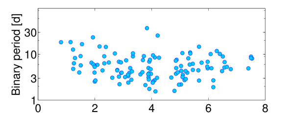
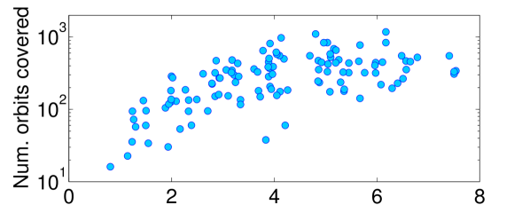
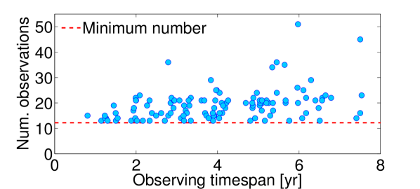
Figure 1: Top: timespan of observations over binaries of different periods. The flat distribution means that our sensitivity to tertiary objects is roughly independent of the binary period. Middle: number of orbits covered for each binary. There is no strict minimum although 86% of binaries have been observed over a timespan covering at least 100 orbits. Bottom: number of observations given to each binary. There is a requirement of at least 13 observations.

2 Observational Campaign

2.1 The CORALIE instrument

CORALIE (Queloz et al. 2001b), is a thermally stabilised (but not pressure-stabilised), high-resolution, fibre-fed spectrograph, mounted on the 1.2m Euler Telescope, a facility belonging to the University of Geneva and installed at ESO’s observatory of La Silla, in Chile. The spectrograph was built on ELODIE’s design (Baranne et al. 1996), which was installed on the 1.93m at OHP and produced the first radial-velocity detection of an exoplanet (Mayor & Queloz 1995). The wavelength solution is obtained by simultaneously illuminating a CCD detector with the star, and with a thorium-argon calibration lamp (Lovis & Pepe 2007). Radial velocities are extracted by cross-correlating the observed spectrum with a numerical mask. The resulting cross-correlation function (CCF) is fitted with a Gaussian profile whose mean corresponds to the radial velocity.

In 2007, CORALIE received a major upgrade allowing it to be more efficient and appropriate for the detection of gas-giants orbiting star as faint as V $\sim 13$ (Wilson et al. 2008; Ségransan et al. 2010). CORALIE has a resolution of order 55 000. Since 2007, we have announced in excess of a 100 transiting planets in collaboration with WASP (e.g. Turner et al. 2016), with several dozens remaining in preparation. Further improvements to the instrument were conducted in November 2014 (change from circular to octagonal fibres), and in April 2015 (wavelength solution now done using a Fabry-Pérot). The first of these two operations produced a small offset in the zero-point of the instrument, of order 10 m s^-1, which remains irrelevant for the precision we obtained on the binary star sample but which needs to be accounted for when deriving orbits for stars with planets (Triaud et al. 2016).

2.2 Target selection and observing campaign

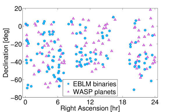
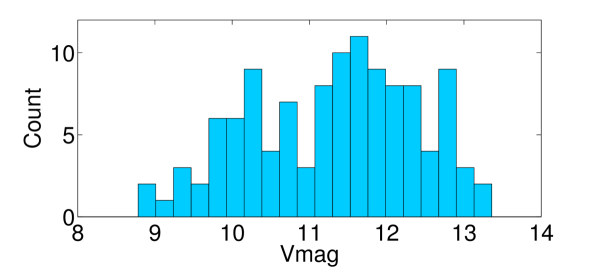
Figure 2: Top: coordinates of each of the EBLM binaries (blue circles) and a comparative distribution of the coordinates of the WASP planets (purple triangles). Bottom: histogram of the visual magnitude.

Stars showing periodic photometric dimmings consistent with the transit of a hot Jupiter are identified by WASP using an algorithm named hunter (Collier Cameron et al. 2007). An analysis of the stellar colours, of their reduced proper-motion and of the duration of the events permits an exclusion of most giant primaries, as well as a preliminary estimate of the stellar radius ($R_{\star}$). The depth of the event, ($D=R^{2}_{\rm p}/R^{2}_{\star}$) leads to an estimate of the transiter’s size. If its radius is consistent with $R_{\rm p}\leq 2.1R_{\rm Jup}$ and no ellipsoidal variation is initially detected then the object is kept and becomes a planet candidate.

The spectroscopic validation of candidates with declination $\delta<+10^{\circ}$ is done using CORALIE (Triaud 2011). We start with two exposures of 1800 seconds, timed to be near the expected radial velocity maximum and minimum. Any amount of radial velocity variation is investigated (even if anti-phased) until the nature of the variation is understood (wrong period from WASP, long period binaries, stellar activity, chance alignment with another eclipsing system, EBLM, etc.). These two spectra are taken on every star except if on the first attempt we detect a secondary set of lines, in which case we classify this object as a double-line binary (SB2), which is no longer observed.

If there is a radial-velocity variation of less than 100 km s^-1 between the two first epochs, but in excess of order 5-6 km s^-1, we classify the object temporarily as part of the EBLM project. Systems with lower variations are followed-up intensively as planetary or brown dwarf candidates, and systems above the criterion are discarded. An amplitude of 100 km s^-1 corresponds approximately to a secondary mass of 0.6 $M_{\odot}$, for an orbital period of 15 days about a $1M_{\odot}$ primary. These requirements therefore contain all the secondaries that we could possibly be interested in.

Figures 1 & 2 graphically represent several characteristics of this current data release. We decided to include all EBLM candidates for which we had at least 13 radial velocity measurement by 2016-03-14, and where the orbital period derived from radial velocities is consistent with that derived from photometry (i.e. all are confirmed to be eclipsing). Thirteen measurements correspond to the bare minimum necessary to adjust up to two Keplerian models through the data, although most of the time this is not needed. Usually, the 11+ measurements that complement the first pair, were obtained at reduced exposures of 600 and 900 seconds (since the semi-amplitudes are much larger than planets), and as high a precision is not required. Many systems received more visits for a variety of reasons including: detection of a tertiary companion, testing whether our uncertainties on periods and eccentricities are robustly determined, and a limited attempt to detect circumbinary objects. Observations were spread over more than three years for the majority of systems, which are mostly contained between V magnitudes 9 and 13, just like the hot-Jupiters we identified. There is a spread in the timespan between roughly one and eight years, because new targets were provided by WASP for spectroscopic follow-up progressively. The amount of time spent on a given target is roughly independent of the binary period, so as to limit any potential biases. We also present the amount of orbits covered (timespan / $P$), indicating that a large majority of targets have been monitored for over 100 orbits. This is important for identifying stellar trends like activity, as well as radial velocity drifts induced by a tertiary star. The EBLMs are spread almost uniformly across the Southern skies in declination and right ascension, with the exception of the galactic plane ($\alpha\sim 6-7$h and $\alpha\sim 16-17$h), which has not been observed by WASP due to heavy stellar crowding.

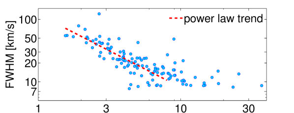
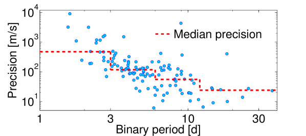
Figure 3: Top: FWHM of the CCF as a function of binary period and a red dashed trend fitted to the data for $P<8$ d. Roughly beyond this period the primary stars are rotating slow enough such that the instrumental broadening dominates the rotational broadening, and truncates any potentially continued trend below 7 km s^-1. Bottom: precision of the radial velocity measurements for each binary as a function of binary period. The red dashed line shows the median precision for all binaries within four coarse period bins, chosen for the later study of triple systems in Sect. 6.4.

Across all 118 targets, we get a median precision of 107 m s^-1. We calculated these values by taking the median photon noise error on the measurements for each system, and quadratically adding an extra term, $\sigma_{\rm add}$ whose estimation is explained in Sect. 3. The precision obtained is not uniform with binary period, as shown in the bottom plot of Fig. 3. The precision of our radial velocity measurements tends to be worse for shorter binary periods, because these stars are forced to rotate synchronously with their orbital periods, owing to tidal forces; this leads to broadened spectral lines. We verify this by plotting the full width at half maximum (FWHM) of the CCF, in the top of Fig. 3 where it can be seen to increase with decreasing binary period. The FWHM that we measure has two dominant components, and is defined as:

$${\rm FWHM}\simeq\sqrt{{\rm FWHM}_{\rm rot}^{2}+{\rm FWHM}_{\rm inst}^{2}},$$ (1)

where ${\rm FWHM}_{\rm rot}$ is the broadening of the absorption lines (and consequently of the CCF) as caused by the rotation of the star, while ${\rm FWHM}_{\rm inst}$ is the instrumental broadening of CORALIE, which depends on its resolution. For CORALIE, ${\rm FWHM}_{\rm inst}\sim 7$, which sets the minimum observable FWHM in Fig. 3. The FWHM_rot increases as the orbital period decreases for objects where the primary star’s rotation period is tidally synchronised to the orbital period of its secondary. This effect saturates at FWHM $\sim 7$ below which we cannot reliably measure the primaries’ rotational broadening.

2.3 Determination of the primaries’ effective temperatures and masses

We have used the empirical colour – effective temperature from Boyajian et al. (2013) to estimate the effective temperatures of the primary stars in these binary systems. We extracted photometry for each target from the following catalogues – B_T and V_T magnitudes from the Tycho-2 catalogue (Høg et al. 2000); B, V, g^′, r^′ and i^′ magnitudes from data release 9 of the AAVSO Photometric All Sky Survey (APASS9, Henden et al. 2015); J, H and K_s magnitudes from the Two-micron All Sky Survey (2MASS, Skrutskie et al. 2006); i^′, J and K magnitudes from the Deep Near-infrared Southern Sky Survey (DENIS, DENIS Consortium 2005). Not all stars have data in all these catalogues.

Our model for the observed photometry has the following parameters – g${}^{\prime}_{0}$, the apparent g^′-band magnitude for the star corrected for extinction; $T_{\rm eff}$ the effective temperature; E$({\rm B}-{\rm V})$, the reddening to the system; $\sigma_{\rm ext}$ the additional systematic error added in quadrature to each measurement to account for systematic errors. For each trial combination of these parameters we use the empirical colour – effective temperature relations by Boyajian et al. (2013) to predict the apparent magnitudes for the binary in each of the observed bands. We assume that the contribution from the low mass companion is negligible at all wavelengths. We used the same transformation between the Johnson and 2MASS photometric systems as Boyajian et al. (2013). We used Cousins I_C as an approximation to the DENIS Gunn i^′ band and the 2MASS K_s as an approximation to the DENIS K band (see Fig. 4; Bessell 2005). We used interpolation in Table 3 of Bessell (2000) to transform the Johnson B, V magnitudes to Tycho-2 B_T and V_T magnitudes. We assume that the extinction in the V band is $3.1\times{\rm E}({\rm B}-{\rm V})$. Extinction in the SDSS and 2MASS bands is calculated using A${}_{\rm r}=2.770\times{\rm E}({\rm B}-{\rm V})$ from Fiorucci & Munari (2003) and extinction coefficients relative to the r^′ band from Davenport et al. (2014).

We used emcee (Foreman-Mackey et al. 2013) to sample the posterior probability distribution for our model parameters. We used the reddening maps by Schlafly & Finkbeiner (2011) to estimate the total line-of-sight extinction to each target, ${\rm E}({\rm B}-{\rm V})_{\rm map}$. This value is used to impose the following (unnormalized) prior on $\Delta={\rm E}({\rm B}-{\rm V})-{\rm E}({\rm B}-{\rm V})_{\rm map}$:

$$P(\Delta)=\left\{\begin{array}[]{ll}1&\Delta\leq 0\\ \exp(-0.5(\Delta/0.034)^{2})&\Delta>0\\ \end{array}\right.$$

The constant 0.034 is taken from Maxted et al. (2014) and is based on a comparison of ${\rm E}({\rm B}-{\rm V})_{\rm map}$ to ${\rm E}({\rm B}-{\rm V})$ from Strömgren photometry for 150 A-type stars.

Finally, primary stellar masses were then estimated by interpolation with in Table B.1 of Gray (2008). The masses we obtain can be found in table LABEL:tab:primary of this paper, as well as values for $T_{\rm eft}$, and $E(B-V)$. The error for the primary mass is calculated by

$$\sigma_{\rm m_{\rm A}}=\sqrt{\left(\sigma_{T_{\rm eff}}\frac{dm_{\rm A}}{dT_{\rm eff}}\right)^{2}+\left(0.06m_{\rm A}\right)^{2}},$$ (2)

where $\sigma_{\rm T_{\rm eff}}$ is the error in $T_{\rm eff}$ and $dm_{\rm A}/dT_{\rm eff}$ is calculated from the empirical mass-effective temperature relation (Torres et al. 2010) by generating 1000 values of $T_{\rm eff}$ from a normal distribution with a standard deviation of $\sigma T_{\rm eff}$. The factor of $0.06$ accounts for the scatter measured around the mass-effective temperature relation (Torres et al. 2010).

The determination of our primaries’ masses is currently coarse and a finer spectroscopic analysis will be done, to update the values that we provide here. We provide detailed results on the model parameters so that the masses for the secondaries can be easily updated when this newer, more accurate information on the primaries is finally released.

Finally, the primary stellar radii were also determined based on Gray (2008). The only purpose of these radii in this paper is to calculate an inclination-based uncertainty in the secondary mass measurement, as will be explained in Sect. 4.1.

3 Treatment of radial velocity data

3.1 Data reduction software

The spectroscopic data were reduced using the CORALIE Data Reduction Software (DRS). The radial velocity information was obtained by removing the instrumental blaze function and cross-correlating each spectrum with a numerical mask corresponding to the spectral type of the primary. The position of all orders were calibrated at the beginning of the night using a tungsten lamp. Masks came in two flavours: G2 and K5. This correlation was compared with the Th-Ar spectrum used as a wavelength-calibration reference (see Baranne et al. (1996) and Pepe et al. (2002) for further information). As the instrument was not pressurised, the wavelength solution changed with variations in atmospheric pressure (approximately equivalent to 100 m s^-1 mbar^-1). The simultaneous calibration Th-Ar (now Fabry-Pérot), on each science frame, accurately corrects instrumental changes. As a precaution, additional calibrations of the wavelength solution were obtained during the night when a drift in excess of 50 m s^-1 is detected.

The CORALIE DRS was built similarly to the DRS for the HARPS, HARPS-North and SOPHIE instruments, and has been shown to achieve remarkable stability, precision and accuracy (e.g. Mayor et al. 2009; Molaro et al. 2013; López-Morales et al. 2014; Motalebi et al. 2015) thanks in part to a revision of the reference lines for thorium and argon by Lovis & Pepe (2007) as well as a better understanding of instrumental systematics (e.g. Dumusque et al. 2015). With a resolving power $R=55\,000$, we obtained a cross-correlation function (CCF) binned in $0.5$ km s^-1 increments. The range over which we computed the CCF was adapted to be three times the size of the full width at half maximum (FWHM) of the CCF on each of the spectra. This ensures that wings of the function are well adjusted by the Gaussian model applied to the CCF.

3.2 Calculating error bars

Uncertainties on individual data points were estimated by the DRS from photon noise alone. CORALIE was stable to $\sim$6 m/s for many years (Marmier 2014), but a recent change from a circular optical fibre to a octagonal at the end of 2014 improved stability to $\sim$3 m/s (Triaud et al. 2016). Given that the majority of the measurements for the EBLM project were taken before the change of fibre, we systematically added 6 m/s of noise, quadratically, to the $1\sigma$ photon noise uncertainties. In the vast majority of cases the photon noise dominates, so the effect of this correction is minimal.

The majority of spectroscopic observations using CORALIE are for a volume-limited Doppler survey to detect planets around bright, Hipparcos-selected, low $v\,\sin\,i_{\star}$ stars (Mayor et al. 2011; Marmier et al. 2013), and the confirmation of the WASP transiting planet candidates (Triaud et al. 2011; Lendl et al. 2014; Neveu-VanMalle et al. 2014). For these two programmes the obtained spectra have high signal-to-noise ratios ($SNR>15$), whereas for the EBLM project, since we mostly deal with shortened exposure times, we frequently obtained lower signal-to-noise spectra ($SNR\sim 3-7$). Furthermore many of our primaries spin rapidly. This decreases the signal-to-noise we obtain on the peak of the CCF, and affects our radial-velocity precision. Our automated error bar estimation was therefore not very well adapted to this new regime of observations for CORALIE, which led to an under-estimation of measurement uncertainties. We corrected the DRS’s uncertainties using an indicator called the span of the bisector slope.

The span of the bisector slope (or the bisector thereafter) measures the asymmetry of the CCF, which reflects the asymmetry of all absorption lines (Queloz et al. 2001a). It has an uncertainty twice the value of the uncertainty achieved on the radial-velocity (Queloz et al. 2001a; Figueira et al. 2013). The bisector is traditionally used to test whether any detected low amplitude radial-velocity variation is caused by a translation of the CCF (as expected for a Doppler reflex motion), instead of caused by a change in the shape of the CCF. This can be produced by stellar activity (leading to an anti-correlation; Queloz et al. 2001a), or by the Doppler reflex motion of a blended, secondary set of lines (creating a correlation; Santos et al. 2002). Whilst this is important to discover exoplanets whose signal can be similar in amplitude to a line shape variation, in our case, the EBLM project, the orbital motion is large ($>$ than the FWHM of the CCF) in addition to not being subject to any detection problem. In our case, we can use the dispersion of the bisector to calculate the true uncertainty on our radial-velocities and correct any under-estimation produced by the DRS. We therefore computed an additional noise term, $\sigma_{\mathrm{add}}$, in the following manner:

$$\sigma_{\mathrm{add}}=\sqrt{{\delta_{\mathrm{bis}}^{2}\over{4}}-\langle\sigma_{\gamma}^{2}\rangle}$$ (3)

where $\delta_{\mathrm{bis}}$ is the rms of the bisector measurements, and $\sigma_{\gamma}$ is the photon noise error. Once $\sigma_{\mathrm{add}}$ is estimated, we check the procedure by finding the mean of the bisector measurements and measuring that the dispersion is compatible with a $\chi^{2}_{\mathrm{reduced}}=1$ where the error terms on the bisector have been updated by quadratically adding:

$$\sigma_{\mathrm{bis}}=2\sqrt{\sigma^{2}_{\mathrm{add}}+\sigma_{\gamma}^{2}}$$ (4)

similarly, the new errors on the radial velocity measurements become:

$$\sigma_{\mathrm{rv}}=\sqrt{\sigma^{2}_{\mathrm{add}}+\sigma_{\gamma}^{2}}$$ (5)

In cases $\delta_{\mathrm{bis}}<\,\langle\sigma_{\gamma}^{2}\rangle$ there is no need for any additional noise term, and hence $\sigma_{\mathrm{add}}$ is set to 0.

3.3 Outlier removal

Several steps were taken to remove outliers. First, all observations with a bisector position more than three interquartile ranges below the first quartile or above the third quartile were automatically removed. Observations such as these with significantly different bisector positions are often indicative of the wrong star accidentally being observed or an anomalously low signal-to-noise, generally owing to poor observing conditions. Any bisector variation within the remaining observations was accounted for with the added $\sigma_{\rm bis}$ noise term described in the previous section. After this automated removal procedure a visual inspection was done of all data series. In particular, there was a check for the consistency of the FWHM, as occasionally the wrong star being observed may still result in a coincidentally similar bisector, but different FWHM. Additionally, some targets received Rossiter-McLaughlin observations during eclipses to measure the projected spin-orbit alignment. These results are to be presented in a future paper and are removed from the data analysis in this paper as the Rossiter-McLaughlin anomaly would likely bias the radial-velocity fit if not modelled accurately. For other observations, care was taken to take them out of eclipse.

4 Orbit fitting

Orbits are fitted using the Yorbit software developed at the University of Geneva. It uses a genetic algorithm to scan a broad parameter space and avoiding falling into local minima. This is coupled with a Markov Chain Monte Carlo to calculate the final orbital solution. Keplerian orbits are fitted independently with no N body interactions between them, although this is something to be developed in the future. This software has been used in particular in many CORALIE and HARPS radial velocity surveys in the past (e.g. Mayor et al. 2011) and is discussed in more detail in Ségransan et al. (2010) and Bouchy et al. (2016).

Table 1: Models ranked by ascending complexity

gray!50 name	num. params.	$P_{1}$	$K_{1}$	$T_{\rm peri,1}$	$f_{1}(m)$	$e_{1}$	$\omega_{1}$	lin.	quad.	cubic	$P_{2}$	$K_{2}$	$T_{\rm peri,2}$	$f_{2}(m)$	$e_{2}$	$\omega_{2}$
Base models
k1 (circ)	4	✓	✓	✓	✓	$--$	$--$	$--$	$--$	$--$	$--$	$--$	$--$	$--$	$--$	$--$
k1d1 (circ)	5	✓	✓	✓	✓	$--$	$--$	✓	$--$	$--$	$--$	$--$	$--$	$--$	$--$	$--$
k1 (ecc)	6	✓	✓	✓	✓	✓	✓	$--$	$--$	$--$	$--$	$--$	$--$	$--$	$--$	$--$
k1d2 (circ)	6	✓	✓	✓	✓	$--$	$--$	✓	✓	$--$	$--$	$--$	$--$	$--$	$--$	$--$
k1d1 (ecc)	7	✓	✓	✓	✓	✓	✓	✓	$--$	$--$	$--$	$--$	$--$	$--$	$--$	$--$
k1d2 (ecc)	8	✓	✓	✓	✓	✓	✓	✓	✓	$--$	$--$	$--$	$--$	$--$	$--$	$--$
Complex models
k1d3 (circ)	7	✓	✓	✓	✓	$--$	$--$	✓	✓	✓	$--$	$--$	$--$	$--$	$--$	$--$
k1d3 (ecc)	9	✓	✓	✓	✓	✓	✓	✓	✓	✓	$--$	$--$	$--$	$--$	$--$	$--$
k2 (circ)	10	✓	✓	✓	✓	$--$	$--$	$--$	$--$	$--$	✓	✓	✓	✓	✓	✓
k2 (ecc)	12	✓	✓	✓	✓	✓	✓	$--$	$--$	$--$	✓	✓	✓	✓	✓	✓

4.1 Calculating the secondary mass

A single Keplerian orbit is characterised by six parameters. There is more than one way to paramaterise this problem. The ones provided by Yorbit are: period, $P$, semi-amplitude, $K$, eccentricity, $e$, time of periapsis passage, $T_{0}$, mass function, $f(m)$ and argument of periapsis, $\omega$. For each of these parameters the Yorbit calculates $1\sigma$ error bars using 5000 Monte Carlo simulations. These parameters are determined independently of the mass of the primary star, $m_{\rm A}$.

Since these are single-lined binaries it is not possible to directly measure the primary and secondary masses. The only mass quantity which we directly measure is the mass function. We must instead use a primary mass inferred from the models described in Sect. 2.3. The secondary mass is then calculated from the mass function by solving the following equation numerically:

$$f(m_{\rm A},m_{\rm B})=\frac{\left(m_{\rm B}\sin I\right)^{3}}{\left(m_{\rm A}+m_{\rm B}\right)^{2}}=\frac{PK^{3}}{2\pi G}.$$ (6)

When evaluating Eq. 6 we take $I=90^{\circ}$, since our binaries are eclipsing. To calculate the error of $m_{\rm B}$ we use the fact that our binaries all have small mass ratios, allowing us to simplify Eq. 6 to $f(m_{\rm A},m_{\rm B})\sim m_{\rm B}^{3}\sin^{3}I/m_{\rm A}^{2}$, for which the error calculation becomes:

$$\frac{\delta m_{\rm B}}{m_{\rm B}}=\frac{1}{3}\left(\frac{\delta f(m_{\rm A},m_{\rm B})}{f(m_{\rm A},m_{\rm B})}+2\frac{\delta m_{\rm A}}{m_{\rm A}}+3\frac{\delta\sin I}{\sin I}\right).$$ (7)

The error in $\sin I$ stems from us not precisely characterising the eclipse impact parameter and hence inclination using the WASP photometry. Based on possible eclipse geometries, the inclination uncertainty is $\delta\sin I=R_{\rm A}/a$. This is a less than 20% contribution to the relative uncertainty in $m_{\rm B}$.

The semi-major axis is calculated using Kepler’s third law,

$$a=\left(\frac{P^{2}G(m_{\rm A}+m_{\rm B})}{4\pi^{2}}\right)^{1/3},$$ (8)

and the error is calculated as

$$\frac{\delta a}{a}=\frac{1}{3}\left(2\frac{\delta P}{P}+\frac{\delta m_{\rm A}+\delta m_{\rm B}}{m_{\rm A}+m_{\rm B}}\right).$$ (9)

The precision in the semi-major axis is always significantly worse than that of the period, due to the uncertainty in the stellar masses.

5 Model selection

We now describe the models which we have fitted to each star and how we choose the most appropriate one.

5.1 Ten different models applied to the data

For each system we try to fit various models to the spectroscopic data and calculate the goodness of fit. The models tested are:

1. k1: a single Keplerian orbit

2. k1d1: a single Keplerian plus a linear drift

3. k1d2: a single Keplerian plus a quadratic drift

4. k1d3: a single Keplerian plus a cubic drift

5. k2: two Keplerians

The drift terms are indicative of an outer third body that is causing the radial velocities to deviate from a single Keplerian over time. Whether we require a linear, quadratic or cubic fit is function of the amplitude of the radial-velocity signal induced by the third body and also the temporal fraction of its orbit covered. When the tertiary orbit is well-covered ($\gtrsim 30\%$), a second Keplerian is generally a better fit. For each of the cases we further tested the goodness of fit with both the binary eccentricity found by Yorbit, and with a forced circular orbit. This means that in total, we adjusted and can test ten different models on our data.

While forcing a circular model, two parameters are dropped: eccentricity, $e$, and argument of periapsis, $\omega$. We denote eccentric and circular models using the parentheses (ecc) and (circ), respectively. The ten models are split into “base” models - k1, k1d1 and k1d2 - and “complex” models - k1d3 and k2, where sometimes the number of measurements approaches the number of degrees of freedom. This distinction is used in the model selection procedure. Note that for a two-Keplerian fit we only ever force the inner binary orbit to be circular, not the tertiary body. In Table 1 we rank all ten models in ascending order of complexity (number of parameters). Ticks are used to indicate the orbital parameters used in each fit, including linear (lin), quadratic (quad) and cubic drift coefficients.

5.2 Using the BIC to select between models

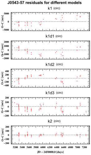
Figure 4: The residuals (O-C) of the radial velocity fit to J0543-57 of five different models with increasing complexity and improved goodness of fit from top to bottom. A k2 (circ) model was ultimately chosen according to our procedure.

We use the Bayesian Information Criterion (BIC; Schwarz 1978) to select the model that provides the optimal balance between goodness of fit and complexity. We assume that the errors in our radial velocity measurements are independent and identically distributed following a normal distribution, so that the BIC can be calculated using

$${\rm BIC}=\chi^{2}+k\ln(n_{\rm obs}),$$ (10)

where $\chi^{2}$ is the weighted sum of the square of the residuals, $k$ is the number of model parameters and $n_{\rm obs}$ is the number of observations. The BIC is constructed to naturally penalise models that are unnecessarily complex and not justified by the data (otherwise known as Ockham’s razor). Whenever choosing between one model and the next most complex (in terms of the number of parameters) we demand that the BIC increases by at least 6 in order to justify the added complexity. This is deemed “strong” evidence in the literature (Kass & Raftery 1995).

Our model selection procedure follows a forward method, where we start with the simplest model and move up in complexity. The steps are as followed:

1. Calculate the BIC for the simplest model: a circular single Keplerian

2. Calculate the BIC for subsequent base models with increasing numbers of parameters, as denoted by the order in Table. 1.

3. Whenever we want to jump from one model to the one with the next highest number of parameters, we demand that the BIC improves (i.e. decreases) by at least 6.

4. Note that k1 (dcc) and k1d2 (circ) both have six parameters. When choosing between those two models simply the smallest BIC is chosen.

5. In some situations the next most complex model may only marginally improve the BIC (i.e. not by 6) but the more complex model after that may be a significant improvement. In these exceptional circumstances one may “jump” to the well-fitting model two ranks of complexity above by improving the BIC by a factor of $2\times 6=12$, or in general $n\times 6$ where $n$ is the number of ranks of complexity you want to move up.

6. For the base model chosen according to the BIC we calculate the reduced $\chi^{2}$ statistic, $\chi_{\rm red}^{2}=\chi^{2}/(n_{\rm obs}-k)$, where $(n_{\rm obs}-k)$ is the number of degrees of freedom. For a good fit to the data we expect $\chi_{\rm red}^{2}\sim 1$.

7. If this value of $\chi_{\rm red}^{2}<2$ then we consider the simple model to be a sufficient fit to the data and do not test any others. This conservative approach helps avoid over-fitting.

8. Alternatively, if $\chi_{\rm red}^{2}>2$ we then test more complex models: k1d3 and k2 (both eccentric and circular). These models are then treated with the same model selection procedure as before. In some cases complex models are tested but a base model is ultimately still chosen.

9. An exception to the above procedure comes in the case of heightened stellar activity. This activity can cause variation in the radial velocity measurements that may be confused for another physical body in the system. This occurs in two cases: J0021-16 and J2025-45. These binaries have $\chi_{\rm red}^{2}$ for the base models of 3.49 and 7.09, respectively, but we do not test more complex models and instead manually assign an appropriate, simpler model. These individual cases are discussed further in Sect. 6.5.

Figure 4 shows our procedure in action on the residuals obtained after removing the most likely parameters for a set model. In this particular case adding a second Keplerian visibly improves the goodness of fit, which also happens in the BIC values. In Table LABEL:tab:BIC we show the data pertaining to the model selection. The BIC of the selected model is highlighted in bold font. For most systems the simple models tested yielded a $\chi_{\rm red}^{2}<2$ and hence no models of further complexity were needed. In Table LABEL:tab:BIC we count the number of binaries fitted to each of the ten models. In the appendices, Table LABEL:tab:params contains the orbital parameters for all of the binaries, taken from the chosen model according to the BIC. For the four binaries where a k2 model was selected we provide the orbital parameters of the tertiary body in Table F.

5.3 Providing upper limits on undetected nested parameters

In reality, no orbit is exactly circular, meaning that the true physical model ought to be eccentric even though statistically that extra degree of complexity in the model is not formally detected. To remedy the issue we provide estimates for upper limits to the eccentricity and the coefficient of linear drift, along with the selected model values, in Table LABEL:tab:params. The values we provide were estimated using the model of higher complexity on that particular parameter. We provide values at 67% confidence by taking the fitted value and adding the $1\sigma$ uncertainty. We do the same for the upper limit of the linear drift coefficient for binaries where a single Keplerian fit was chosen.

6 Results

6.1 Summary

In total we analysed 118 eclipsing binaries. Table LABEL:tab:BIC shows the number of stars for which each model was selected using the BIC. The results of the model fits to individual stars are given in a series of tables in the appendices to the paper. First, in Table LABEL:tab:BIC we demonstrate our model selection procedure based on the Bayesian Information Criterion and reduced $\chi^{2}$ statistic. The chosen model is given in this table and the BIC for that model is highlighted in bold. For most systems the simple models tested yielded a $\chi_{\rm red}^{2}<2$ and hence no models of further complexity were needed. The flag column has three different flags: “drift” indicating that a linear, quadratic or cubic drift was the best fit to the data, “triple” for the four systems where we fitted two Keplerian orbits to the triple star system and “active” for the two systems showing signs of stellar activity.

The orbits of the best-fitting models and their residuals are shown in Appendix E.

Contained in in Table LABEL:tab:params are the orbital parameters for all of the binaries. For each parameter we show both the measured value and the uncertainty. The uncertainty is the value inside the brackets and corresponds to the final two digits of the measured value. For example, for J0008+02 $P=4.7222907(63)$ days, which means $P=4.7222907\pm 0.0000063$ days. This table includes the calculated primary and secondary masses. More detailed parameters for the primary stars are shown in Table LABEL:tab:primary. The J and V magnitudes come from the NOMAD survey and the R magnitude comes from 2MASS. An exception is that for three targets, J1934-42, J1509-10 and J2353-10, no Vmag was available from NOMAD so it was calculated as a function of the primary mass using models by Baraffe et al. (2015) at an age of 1 Gyr.

For the four targets with characterised tertiary orbits we provide their orbital parameters and plots of the radial velocity fits in Appendix F.

Parameters for the secondary stars are shown in Table LABEL:tab:secondary. The error in the secondary mass is predominantly due to uncertainties in the primary mass and orbital inclination, and not the radial velocity semi-amplitude. Unlike the primary star, which has measured magnitudes, the secondary magnitudes are all calculated using the Baraffe et al. (2015) models. Values for the V, R and J magnitudes are given at ages of 1 Gyr and 5 Gyr. This is because we do not have accurate estimates for the true ages of the systems, although we note that the magnitude difference is small.

Finally, in Table LABEL:tab:obs are various observational parameters for the binaries. The period $P$ and times $T_{\rm 0,pri}$ and $T_{\rm 0,sec}$ (for the primary and secondary eclipses) are taken from the radial velocity fit, not the WASP photometry.

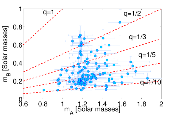
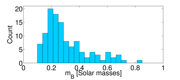
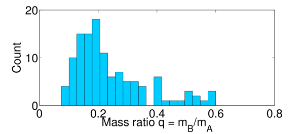
Figure 5: Top: mass ratio $q=m_{\rm A}/m_{\rm B}$ for each of the binaries including error bars. The fractional error of the secondary is generally similar to that of the primary, and consequently the absolute error for the secondary is invisibly small on this plot for small $m_{\rm B}$. Red dashed lines correspond to mass ratios of $1$, $1/2$, $1/3$, $1/5$ and $1/10$. Middle: histogram of the secondary mass. Bottom: histogram of the mass ratio.

6.2 Primary and secondary masses and magnitudes

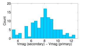
Figure 11: Histogram of the difference between the secondary and primary visual magnitudes, using the data provided in Table LABEL:tab:obs. Primary Vmag values come from the NOMAD survey, except for three binaries where they are calculated using models from Baraffe et al. (1998) at an age of 1 Gyr. All secondary Vmag values are calculated using Baraffe models with a 1 Gyr age.

We now demonstrate visually some of the results in our sample. In Figure 5 we show the primary and secondary masses in our sample. It is seen that 60 of our binaries (50% of the sample) have mass ratio $q<0.2$, and, 34 (31%) companions have masses $m_{\rm B}<0.2M_{\odot}$. A consequence of these small mass ratios is that our secondary stars are all between 3.1 and 12.6 magnitudes fainter than the primary stars, and hence we only observe a single-line spectroscopic binary. A histogram of this difference in magnitudes is shown in Fig. 11.

Figure 7 shows a combined WASP/EBLM mass spectrum for objects creating photometric eclipses compatible with sizes $<2.1R_{\rm Jup}$. We usually give a “WASP” identifier for all sub-stellar objects (planets and brown dwarfs). We collected all objects with WASP identifiers that are public and were observed with the CORALIE spectrograph and added all stellar companions in this paper. In overall this means 143 substellar objects and the 118 stellar companions presented in this paper. One of our sub-stellar companions, WASP-30 (Triaud et al. 2013) falls within the brown dwarf range.

We compare our preliminary results to the 50pc mass spectrum shown in Grether & Lineweaver (2006). To do this, we normalise their histogram to our number of sub-stellar objects with masses superior to $1M_{\rm Jup}$. From Fig. 7, we see that our mass spectrum covers a broader range in the planetary masses (although at low masses we are most likely incomplete), and does not cover stars as massive (due to the restriction of our survey). Over the common range between Grether & Lineweaver (2006) and us, we have a resolution that is twice better. The results are broadly consistent, but differ in an interesting way. The brown dwarf desert derived from the WASP and EBLM results appears to stretch deeper into the planetary domain than the result of Grether & Lineweaver (2006). We find that in our results, massive gas-giants ($\sim 3-13M_{\rm Jup}$) appear less abundant.

The reason for the discrepancy with the Grether & Lineweaver (2006) results is that their work probed planets on wider orbits $a<\lesssim 10$ AU, whereas EBLM and WASP are typically sensitive to $a<0.2$AU. Whatever process(es) is(are) important in shaping the hot Jupiters population, it(they) favour(s) smaller mass gas-giants. This was also noted in Udry et al. (2003).

The entire EBLM sample contains over 200 binaries (of which only 118 are presented here); the WASP survey is still on-going. Once those results are all published we will revisit this mass spectrum. In particular, in the future we will be able to compare the relative abundance of close hot-Jupiters, brown dwarfs and M-dwarfs. On this occasion, we will also produce a more thorough analysis and debiasing of the spectrum.

6.3 Eccentricities

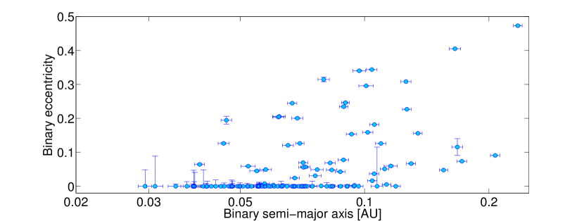
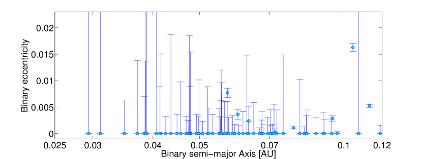
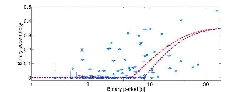
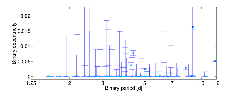
Figure 6: The eccentricity of the eclipsing binary as a function of semi-major axis (top two plots) and period (bottom two plots). Plots b and d are zoomed versions of the a and c, respectively, showing the tightest binaries ($P_{\rm bin}<12$ d) with eccentricities compatible with zero. In the top plot the error in semi-major axis is shown, but this is excluded in the zoomed version for clarity. In the third figure (period vs eccentricity, not zoomed) we use dashed lines to denote fits using the Meibom & Mathieu function in Eq. 11. The purple dashed line is a fit to all of the data where $P_{\rm cut}=8.9$ days, whilst the red dashed line is a fit to all binaries with $M_{1}<1.3M_{\odot}$ and no sign of a tertiary companion. In this latter case $P_{\rm cut}=7.0$ days.

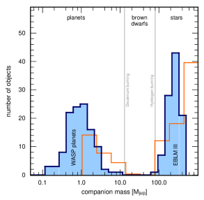
Figure 7: In dark blue, the observed mass spectrum from the WASP planet survey and the EBLM binaries released in this paper.. The orange histogram depicts the results from Grether & Lineweaver (2006), normalised to the number of WASP and EBLM objects heavier than $1M_{\rm Jup}$. The vertical grey lines denote the rough mass limits for Deuterium burning ($13M_{\rm Jup}$) and Hydrogen burning ($80M_{\rm Jup}$). There is an evident deficit of objects between these two limits, which corresponds to the realm of brown dwarfs.

In Figure 6 we show the eccentricity of our systems as a function of the semi-major axis (top two plots) and period (bottom two plots). For the unzoomed $P$ vs $e$ plot we show a fit to the data using the Meibom–Mathieu function (Meibom & Mathieu 2005), which is presented in Sect. 7. For both the semi-major axis and period we show zoomed versions of the plots for eccentricities between 0 and 0.022. There are many binaries for which we can constrain their orbits to being circular within these small bounds of eccentricity. Furthermore, there are some binaries for which we actually measure eccentricities that are small but significantly non-zero. This high precision is by virtue of using the CORALIE instrument with planet-finding precision to observe much larger amplitude binaries. The smallest significantly non-zero eccentricity measured is $e=0.00108\pm 0.00017$ for J0353+05. The most precisely measured eccentricity is $e=0.051004\pm 0.000086$ for J0042-17. These results are expanded upon in Figure 8a which is a histogram of the eccentricity precision obtained in the EBLM program. For half of our targets we can constrain eccentricities to a precision of 0.0025. For 29% we obtain a precision better than 0.001 and for 14% a precision better than 0.0005.

The periods of our binaries are measured to an even better precision. In Figure 8b is a histogram of the precision obtained on the binary period, shown in a scale of seconds. Half of the sample have a period measured to better than 1.4 seconds. As a percentage error, 50% of our targets have their period measured to better than 0.00031%. with the worst being 0.047% for J0629-67. Our highly precise periods are a result of both the high resolution CORALIE instrument and the fact that all orbits have been observed for a timespan of at least $16P_{\rm bin}$ and 86% are observed over a timespan of more than $100P_{\rm bin}$.

The longest period binary for which we measure a zero eccentricity is J1008-29 with a 10.4 day period and $e<0.0016$.

The implications of our measured eccentricities as a function of period and semi-major axis are discussed in Sect. 7.

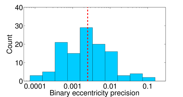
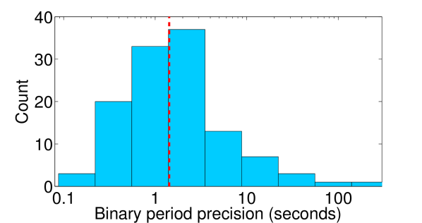
Figure 8: Top: histogram of the precision of the eccentricity for all of our 118 binaries. For models where an eccentricity is favoured it is the $1\sigma$ error bar. For models where a circular solution is favoured it is the upper limit, which is equal to the fitted eccentricity value plus the $1\sigma$ uncertainty. The vertical red dashed line is the median precision of 0.0025. Bottom: histogram of the precision of the binary period, in seconds. The red dashed line is the median precision of 1.4 seconds. We emphasise that the period precision is obtained purely by the radial velocity fit, not from the eclipse timing.

6.4 Triple star systems

According to Table LABEL:tab:BIC there are 21 systems fitted with a model other than a single Keplerian (circular or eccentric). All solutions fitted with a drift or second Keplerian are indicative of a third body, most likely a tertiary star but possibly a circumbinary brown dwarf or massive planet. Our overall tertiary rate is $21/118=17.8\%$. In Fig. 9 we plot the percentage of systems with indications of a close tertiary companion as a function of inner binary period (blue solid line). Bin edges are chosen to match the study of Tokovinin et al. (2006): 3, 6, 9, 12, 40. This plot indicates a roughly flat rate of triples as a function of $P$. This contrasts with the results of Tokovinin et al. (2006) (orange dash-dotted line) in two ways. First, our results are significantly lower at all binary periods. The cause of this is however simple. Our only indicator of a third star is an additional radial-velocity signal, and this is only sensitive to close triples (estimate period range) and can miss tertiary stars with inclinations near zero. By contrast, Tokovinin et al. (2006) was an imaging survey of known spectroscopic binaries, so whilst it may miss some very tight triple systems it is sensitive to a much larger range.

Second, one of the most important results of Tokovinin et al. (2006) was the sharp dependence of tertiary fraction on binary period. This has been interpreted as evidence for the formation of close binaries via Kozai-Lidov cycles followed by tidal circularisation (Lidov 1962; Kozai 1962; Mazeh & Shaham 1979; Fabrycky & Tremaine 2007) and this is different to the flat distribution seen in our raw triple fraction. If the distributions of tertiary periods and masses are uncorrelated with the inner binary period, then on average the slope of the radial velocity drift would be independent of the inner binary period. However, our detectability of this radial-velocity drift is not uniform with binary period in our sample. As shown in the top of Fig. 1, the observing time spent on a given target is not dependent on the binary period, so this does not introduce a bias. However, a significant bias is the trend of decreasing precision with closer binaries. This is due to tidal locking leading to broadened spectral lines, as discussed in Sect. 2.2 and evidenced in Fig. 3. For $P_{\rm bin}<3$ days there are 20 binaries and the median precision obtained is 477 m/s. Between 3 and 6 days the median precision improves to 118 m/s. For 6 to 12 day binaries there is a further improvement to 56 m/s and for our 10 binaries with a period longer than 12 days we have an excellent median precision of 24 m/s. This strong bias hurts our ability to detect tertiary companions to very close binaries. This was not shared with Tokovinin et al. (2006), who used imaging.

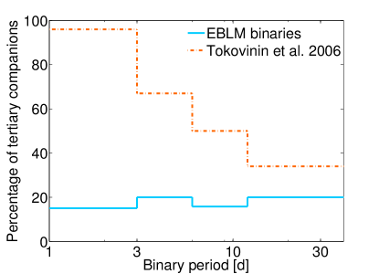
Figure 9: Percentage of our EBLM binaries with a tertiary companion (blue solid line). Binaries are said to have a tertiary companion if the best fitting radial velocity model is not a single Keplerian. For comparison we show the results of the Tokovinin et al. (2006) imaging survey of close spectroscopic binaries (orange dashed line).

Of the 21 binaries identified as having a tertiary companion in four cases our observations allow a characterisation of the tertiary orbit: J0543-57, J1146-42, J2011-71 and J2046-40. These four triples have outer periods of 3062, 260, 663 and 5584 days, respectively. All orbital parameters are provided in Table F in Appendix F. In this appendix we also provide orbits of both the inner binary and outer tertiary and a top-down view. J1146-42 in particular, with three stars within $\sim 1$ AU (modulo $\sin i_{\rm C}$), is a rare tight triple star system. We note that for the best fitting model $\chi_{\rm red}^{2}=15.06$ which is actually the worst in our sample, which may seem surprising given the precision obtained is so high (median 18 m s^-1) owing to its brightness (Vmag$=10.3$) and long inner period ($P=10.47$ days). We suggest that the cause of these large residuals is a Newtonian perturbation between the two orbits causing them to become non-Keplerian, which is not accounted for within Yorbit. This arises because the inner and outer orbits are close: $a_{\rm out}/a_{\rm in}=9.1$. Our observing timespan of 3.34 years and high precision make us sensitive to these perturbations. It is a future task to analyse the orbital dynamics of these close triple systems and try to exploit them to calculate additional parameters in the system, such as the mutual inclination between the two orbits (e.g. Correia et al. 2010).

It is also likely that the ongoing GAIA astrometric survey will provide additional orbital constraints on these triple systems.

6.5 Active systems

Throughout the history of radial-velocity surveys for extra-solar planets, stellar activity has often contrived to confuse observers by creating spurious radial velocity variations that may be mistaken as planets (e.g. Queloz et al. 2001a). Fortunately in a survey of binaries, the amplitude of the Keplerian signal is tens of km s^-1, which is higher by orders of magnitude compared to stellar activity. From this perspective there is therefore no doubt about the existence of our binaries. What stellar activity may do, however, is inhibit our ability to detect smaller amplitude effects such as radial-velocity drifts indicative of a third star, as these may be of a low amplitude of only tens of metres per second.

In exoplanet studies, a classic diagnostic for stellar activity is the span of the bisector slope (Queloz et al. 2001a; Figueira et al. 2013), which we use here as well. An anti-correlation between a motion in radial-velocity and in the slope of the bisector indicates a distortion of the absorption lines, caused by stellar activity.

For two of our binaries we see clear signs of stellar activity: J0021-16 and J2025-45. In Fig. 10(a) we plot for J0021-16 the residuals from a single Keplerian fit and in Fig. 10(b) for a single Keplerian plus linear drift. When only a single Keplerian is fitted there is a clear linear negative trend between the residuals and the bisector. However, if we look in more detail we see that the more recent points, denoted in purple, have a systematic shift in bisector to the left in comparison with the older points. This indicates that whilst there is stellar activity present throughout all of the observations, there is an additional source of the residuals. When a linear drift is added, we see in Fig. 10(b) that the latest points in purple now overlap the other points. We conclude that this system has both stellar activity and a tertiary stellar companion inducing a drift. This illustrates the advantage of our long observing baseline, which was 5.34 yr for this target. The case is different for J2025-45, for which there is no discernible difference in the bisector-residuals correlation between the old and new observations. This is not due to a lack of time spent on the target, as the observations span a total of 5.45 yr. We assign a single eccentric Keplerian fit to this target.

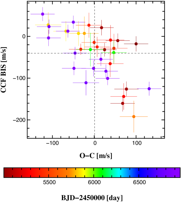
(a) J0021-16; k1

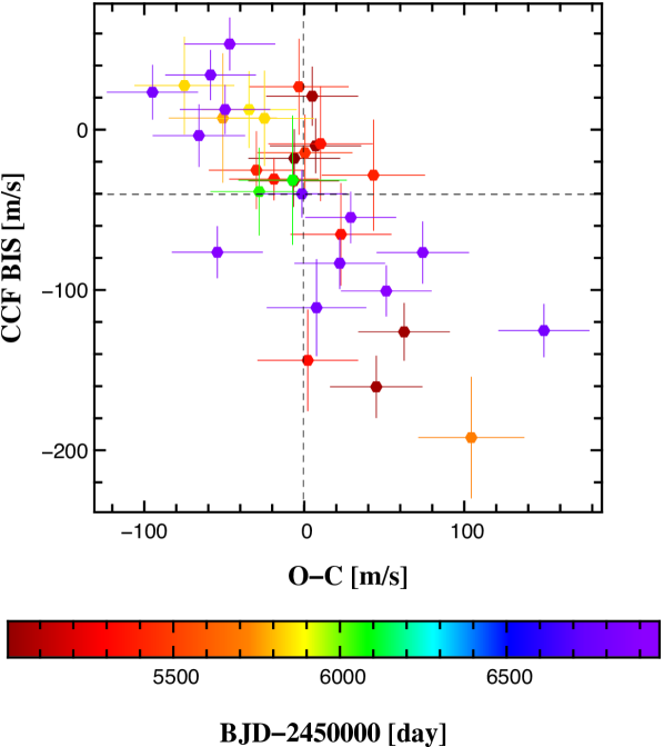
(b) J0021-16; k1d1

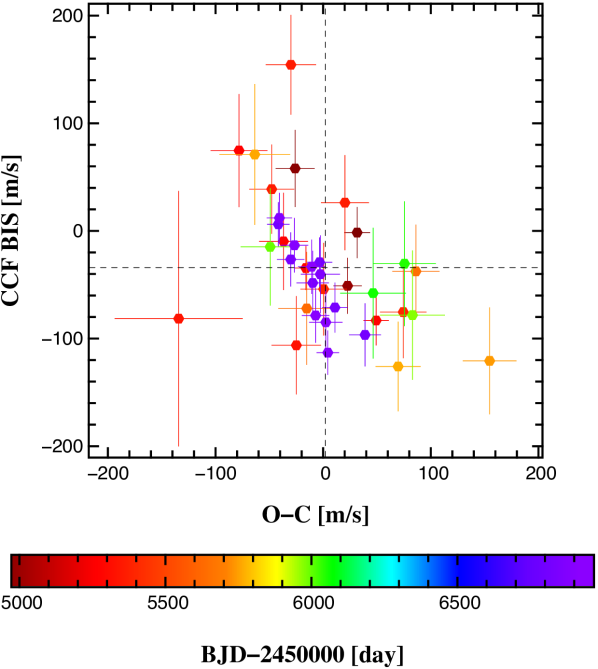
(c) J2025-45; k1

Figure 10: Correlation between the bisector and residuals to an eccentric single Keplerian fit for two of our targets showing signs of stellar activity: J0021-16 and J2025-45. This negative linear trend is an indicator of stellar activity.

7 A discussion on tidal evolution

One of the scientific advantages of having very precise eccentricities and periods is to allow investigations into tidal interactions. A future work is planned to exploit the results of the EBLM survey in more details and to better our understanding tidal evolution in close binaries. For now, we discuss some of the first order implications that our results may have.

Tidal interactions between two close stars have several effects (Zahn 1975, 1977):

• Synchronisation of the rotation and orbital periods for circular orbits (pseudo-synchronisation for eccentric orbits (Hut 1981);

• Alignment of the orbital and spin axes of the stars

• Circularisation of the orbit

In the plot of FWHM and precision as a function of the binary period (Figure 3) we saw evidence for tidal synchronisation, which manifests itself as spectral lines being more broadened with a reduced orbital period. Measurements of the Rossiter–McLaughlin effect, which probe the projected obliquity of the orbit, will serve to help better understand the strength of tidal realignment, and confront theoretical expectations (e.g. Anderson et al. 2016).

These are to be presented in a future paper. Finally, the plots of binary eccentricity as a function of semi-major axis and period in Figure 6 allow us to probe the circularisation of the orbit. By eye, it is evident that there is a trend of increased eccentricity with semi-major axis and period, which is expected since tides are mostly effective over very short distances. Binaries are not expected to form on primordially circular orbits. Rather, they circularise over time (e.g. Mazeh & Shaham 1979; Fabrycky & Tremaine 2007; Bate 2012). A consequence of this is that one may define a cut-off period, $P_{\rm cut}$, above which orbits are found eccentric. Meibom & Mathieu (2005) provided a means of measuring $P_{\rm cut}$ as follows:

$$e(P)=\left\{\begin{array}[]{ll}0.0&\mbox{if }P\leq P_{\rm cut}\\ \\ \alpha\left(1-e^{\beta(P_{\rm cut}-P)}\right)^{\gamma}&\mbox{if }P>P_{\rm cut}\end{array}\right.,$$ (11)

where the constants were calculated to be $\alpha=0.35$, $\beta=0.14$ and $\gamma=1.0$. The value of $\alpha$ is defined based on the mean eccentricity of all field binaries of periods greater than 50 days being 0.35, whilst $\beta$ and $\gamma$ were shown to optimise the fit. In Figure 6 we include two versions of our fitted Eq. 11. First, we make a fit to all of the data, and calculate $P_{\rm cut}=8.9$ days. Second, we make a fit to only the binaries where $M_{\rm A}<1.3M_{\odot}$ and there is no sign of a tertiary companion. This second adjustment yields a more accurate $P_{\rm cut}=7.0$ days. We base our preference on the following. Heavier stars have a radiative outer envelope, rather than a convective one (Pinsonneault et al. 2001). Tidal dissipation in radiative envelopes is less efficient, which causes tidal circularisation to be slower (similar arguments have been invoked in the exoplanet literature; Albrecht et al. 2012; Dawson 2014). Additionally, outer tertiary companions may induce some eccentricity in the inner binary via secular perturbations.

Our $P_{\rm cut}$ result comes in conflict with other estimates discussed in the literature and compiled in Meibom & Mathieu (2005) with an update in Milliman et al. (2014). Results obtained in the field (Duquennoy & Mayor 1991), the halo (Latham et al. 2002), in M 67 (Mathieu et al. 1990) and NGC 188 (Mathieu et al. 2004), all with ages $>1$ Gyr, are found with $P_{\rm cut}>10$ days. The only exception is NGC 6819 (Milliman et al. 2014) whose value $P_{\rm cut}=6.2\pm 1.1$ days is consistent with ours. This is also consistent with results on young open clusters ($<100$ Myr), where $P_{\rm cut}$ is found around 8 days (Melo et al. 2001). The reason for disagreement between our value and the bulk of other results on old populations is not presently known. A contributing factor may be that our survey is, by design, biased towards small mass ratio binaries, and the circularisation timescale is dependent on the mass ratio (Zahn 1977, 1978). Past surveys may also suffer from small number statistics and a poorer precision on eccentricities than what we can produce nowadays. This preliminary result is consistent with there only being marginal tidal evolution during the Main Sequence. We have another 100+ binary systems under observation at the moment and will update our $P_{\rm cut}$ and analysis once observations on those are completed.

8 Conclusion

We present the spectroscopic orbits of 118 stellar systems, all eclipsing single-line binaries. We produce that sample in order to map out the sky position of eclipsing systems mimicking transiting hot-Jupiters. This will be of great help in the advent of large scale exoplanet surveys such as TESS and PLATO. In addition, this sample can be used as a comparison to hot-Jupiters for a host of topics that are detailed in the introduction.

Our release of these systems opens multiple opportunity for further research, for instance to detect tertiary companions with direct imaging, astrometry or eclipse timing variations. As high-resolution, near-infrared spectrographs are coming online, it will become feasible to transform our single-line binaries into double-line systems and derive accurate masses and radii (Torres & Ribas 2002; Brogi et al. 2012; Rodler et al. 2012). As part of the efforts of our team, we will double the current sample of eclipsing low-mass binaries (we are currently acquiring data to reach a minimum of 13 radial-velocity measurements), measure some primary eclipses of secondaries with mass $<0.2M_{\odot}$, prepare a publication on the Rossiter–McLaughlin effect of 20 of our binaries. .

We derive orbital periods with a precision of order one second and compute eccentricities well below 1%. This is thanks to longterm observations using a stable, high precision spectrograph usually employed in the discovery of exoplanets. We use our results to carry-out a preliminary investigation of the strength of tidal forces in stars. To a first order, we find that binaries in the field have a similar eccentricity distribution to pre main-sequence binaries, This is consistent with there being marginal tidal evolution over a main sequence lifetime, although further investigation is needed to make a definitive statement.

Ordering our sample as a function of mass, and adding the results, with the same instrument, from WASP and CORALIE on exoplanets, we construct a preliminary mass spectrum. Its appears to show a deficit of planets with masses $>3M_{\rm Jup}$ compared to earlier results considering wider orbital separations.

For 21 of our systems there is a significant indication of an outer tertiary companion, most likely stellar in nature and long period. For four systems we are actually able to characterise the tertiary orbit, including one system with three stars packed within 1 astronomical unit. We will also intensify our monitoring of a subset of our systems in search of circumbinary gas-giants, in a connected program known as BEBOP

Nota Bene

We used the Barycentric Julian Dates in our analysis. Our results are based on the equatorial solar and jovian radii and masses taken from Allen’s Astrophysical Quantities (Cox 2000)

• The Two Micron All Sky Survey (2MASS), which is a joint project of the University of Massachusetts and the Infrared Processing and Analysis Center/California Institute of Technology, funded by the National Aeronautics and Space Administration and the National Science Foundation (Skrutskie et al. 2006).

• The Naval Observatory Merged Astrometric Dataset (NOMAD), which is project of the US Naval Observatory (Monet et al. 2003).

• The Tycho2 catalog (Høg et al. 2000).

• The AAVSO Photometric All-Sky Survey (APASS), funded by the Robert Martin Ayers Sciences Fund (Henden et al. 2015)

Appendix A Model Selection using the Bayesian Information Criterion

Table 2: Bayesian Information Criterion (BIC) with selected model in bold

System				Base Models							Complex Models
				k1		k1d1		k1d2			k1d3		k2
name	num.	chosen	flag	circ	ecc	circ	ecc	circ	ecc	$\chi_{\rm red}^{2}$	circ	ecc	circ	ecc	$\chi_{\rm red}^{2}$
	obs.	model		4 params.	6 params.	5 params.	7 params.	6 params.	8 params.		7 params.	9 params.	10 params.	12 params.
EBLM J0008+02	25	k1d2 (ecc)	drift	455341	9907	423270	229	432023	55	1.71	–	–	–	–	–
EBLM J0017-38	13	k1 (circ)		22	27	24	29	26	30	1.33	–	–	–	–	–
EBLM J0021-16	34	k1d1 (circ)	active	221	178	119	122	122	121	3.49	–	–	–	–	–
EBLM J0027-41	14	k1 (ecc)		310	20	247	23	240	25	0.54	–	–	–	–	–
EBLM J0035-69	21	k1 (ecc)		41514	40	39897	41	41171	42	1.42	–	–	–	–	–
EBLM J0040+01	20	k1 (ecc)		13223	37	13051	39	12830	46	1.34	–	–	–	–	–
EBLM J0042-17	17	k1 (ecc)		541568	34	522070	37	598991	39	1.57	–	–	–	–	–
EBLM J0048-66	18	k1 (ecc)		2897	22	5777	25	3767	26	0.42	–	–	–	–	–
EBLM J0057-19	18	k1 (circ)		24	23	21	23	26	26	0.9	–	–	–	–	–
EBLM J0104-38	16	k1d1 (ecc)	drift	92	41	52	28	58	29	0.92	–	–	–	–	–
EBLM J0109-67	21	k1 (ecc)		523	34	531	37	551	40	1.07	–	–	–	–	–
EBLM J0218-31	45	k1d2 (circ)	drift	1886	1789	276	275	80	86	1.46	–	–	–	–	–
EBLM J0228+05	15	k1 (circ)		16	21	19	24	24	27	0.48	–	–	–	–	–
EBLM J0239-20	21	k1d1 (circ)	drift	45	48	35	41	37	44	1.23	–	–	–	–	–
EBLM J0247-51	19	k1 (circ)		34	38	36	41	37	42	1.48	–	–	–	–	–
EBLM J0310-31	15	k1 (ecc)		9932207	24	9939367	27	9756689	27	0.9	–	–	–	–	–
EBLM J0315-24	21	k1 (circ)		32	37	34	40	37	43	1.15	–	–	–	–	–
EBLM J0326-09	14	k1 (circ)		21	23	22	25	24	27	1.02	–	–	–	–	–
EBLM J0339+03	15	k1 (circ)		26	30	29	35	27	28	1.37	–	–	–	–	–
EBLM J0351-07	21	k1 (ecc)		1488	35	1437	38	1945	41	1.12	–	–	–	–	–
EBLM J0353+05	51	k1d3 (ecc)	drift	52221	50336	1593	2327	145	127	2.23	94	69	102	72	0.81
EBLM J0353-16	29	k1 (ecc)		621	59	590	63	746	67	1.69	–	–	–	–	–
EBLM J0400-51	13	k1 (circ)		15	17	17	20	22	22	0.52	–	–	–	–	–
EBLM J0425-46	14	k1 (ecc)		20607	18	20581	21	21047	23	0.27	–	–	–	–	–
EBLM J0432-33	21	k1 (circ)		25	28	28	31	36	34	0.74	–	–	–	–	–
EBLM J0440-48	21	k1 (circ)		25	29	21	26	23	28	0.77	–	–	–	–	–
EBLM J0443-06	20	k1 (ecc)		383	20	386	23	393	26	0.15	–	–	–	–	–
EBLM J0454-09	19	k1 (circ)		33	37	36	40	39	43	1.4	–	–	–	–	–
EBLM J0500-46	13	k1 (ecc)		12029	23	12138	37	13398	48	1.02	–	–	–	–	–
EBLM J0502-38	16	k1 (circ)		17	21	20	23	23	26	0.5	–	–	–	–	–
EBLM J0504-09	22	k1 (circ)		49	52	52	55	55	57	2.05	58	54	42	48	2.42
EBLM J0518-39	21	k1 (circ)		34	35	37	38	40	42	1.28	–	–	–	–	–
EBLM J0520-06	14	k1 (circ)		14	17	17	20	20	22	0.37	–	–	–	–	–
EBLM J0525-55	14	k1 (circ)		40	32	63	40	126	35	2.93	210	37	35	32	2.72
EBLM J0526+04	14	k1 (circ)		25	27	31	30	28	30	1.48	–	–	–	–	–
EBLM J0526-34	21	k1 (ecc)		83506	37	81877	39	81525	40	1.26	–	–	–	–	–
EBLM J0540-17	18	k1d3 (ecc)	drift	3785	3391	329	336	63	57	3.79	140	38	38	43	1.34
EBLM J0543-57	35	k2 (circ)	triple	205949	200239	29371	27488	1537	1178	42.57	514	211	59	62	0.95
EBLM J0546-18	21	k1 (circ)		28	30	25	29	29	32	0.93	–	–	–	–	–
EBLM J0608-59	21	k1 (ecc)		166959	28	146603	31	205515	35	0.68	–	–	–	–	–
EBLM J0610-52	19	k1 (circ)		14	19	16	22	19	25	0.13	–	–	–	–	–
EBLM J0621-46	19	k1 (circ)		14	19	17	22	19	24	0.13	–	–	–	–	–
EBLM J0621-50	25	k1 (circ)		45	39	48	41	51	44	1.52	–	–	–	–	–
EBLM J0623-27	14	k1 (ecc)		2782	21	2399	24	3847	26	0.66	–	–	–	–	–
EBLM J0625-43	21	k1 (circ)		28	30	31	33	34	34	0.93	–	–	–	–	–
EBLM J0627-67	24	k1 (ecc)		21450	26	21452	29	21561	32	0.38	–	–	–	–	–
EBLM J0627-59	13	k1 (circ)		15	19	20	19	36	21	0.56	–	–	–	–	–
EBLM J0629-67	15	k1d3 (ecc)	drift	3564	1508	188	150	286	71	7.01	233	62	277	54	6.35
EBLM J0642-60	16	k1 (circ)		25	26	28	28	31	31	1.2	–	–	–	–	–
EBLM J0645-61	36	k1 (ecc)		2249	28	2241	32	2550	35	0.22	–	–	–	–	–
EBLM J0645-26	22	k1 (ecc)		3296	23	3167	26	3525	28	0.26	–	–	–	–	–
EBLM J0649-27	20	k1 (circ)		32	27	34	30	38	33	1.24	–	–	–	–	–
EBLM J0650-34	13	k1 (circ)		12	15	15	18	18	21	0.19	–	–	–	–	–
EBLM J0659-61	19	k1d2 (ecc)	drift	63	65	72	41	75	35	1.01	–	–	–	–	–
EBLM J0700-30	13	k1 (circ)		17	21	26	31	36	25	0.78	–	–	–	–	–
EBLM J0709-52	16	k1 (ecc)		3943	18	3958	21	4061	23	0.18	–	–	–	–	–
EBLM J0801+02	13	k1 (circ)		21	25	23	27	25	30	1.19	–	–	–	–	–
EBLM J0851+05	16	k1 (circ)		17	22	19	24	21	26	0.46	–	–	–	–	–
EBLM J0855+04	22	k1 (ecc)		545	28	547	30	553	33	0.6	–	–	–	–	–
EBLM J0941-31	21	k1 (ecc)		24573	47	23997	52	32212	47	1.89	–	–	–	–	–
EBLM J0948-08	26	k1d2 (ecc)	drift	120780	2705	92104	154	95172	49	1.3	–	–	–	–	–
EBLM J0954-23	21	k1 (ecc)		648	28	621	31	768	34	0.67	–	–	–	–	–
EBLM J0954-45	23	k1 (ecc)		184316	33	179057	36	201067	39	0.86	–	–	–	–	–
EBLM J0955-39	23	k1 (circ)		34	38	36	44	34	40	1.11	–	–	–	–	–
EBLM J1007-40	21	k1 (circ)		17	23	19	25	22	28	0.28	–	–	–	–	–
EBLM J1008-29	13	k1 (circ)		12	16	14	19	17	21	0.15	–	–	–	–	–
EBLM J1013+01	21	k1 (circ)		34	38	37	40	41	43	1.31	–	–	–	–	–
EBLM J1014-07	24	k1d1 (ecc)	drift	66406	316	66383	34	67380	36	0.71	–	–	–	–	–
EBLM J1023-43	16	k1 (circ)		14	19	16	21	20	24	0.25	–	–	–	–	–
EBLM J1034-29	24	k1 (circ)		27	32	29	34	33	35	0.73	–	–	–	–	–
EBLM J1037-25	20	k1 (ecc)		29835	33	29440	36	32168	36	1.05	–	–	–	–	–
EBLM J1037-45	13	k1 (circ)		11	16	13	18	17	21	0.07	–	–	–	–	–
EBLM J1038-37	13	k1d3 (ecc)	drift	2998	2583	420	374	68	42	4.29	42	27	28	32	1.05
EBLM J1104-43	18	k1 (circ)		14	19	16	22	20	25	0.15	–	–	–	–	–
EBLM J1105-13	17	k1 (circ)		23	26	25	29	26	31	0.87	–	–	–	–	–
EBLM J1116-32	22	k1 (circ)		21	26	24	29	28	31	0.46	–	–	–	–	–
EBLM J1116-01	14	k1 (circ)		13	18	15	20	18	22	0.28	–	–	–	–	–
EBLM J1141-37	21	k1 (circ)		27	31	29	33	32	36	0.87	–	–	–	–	–
EBLM J1146-42	13	k2 (ecc)	triple	674940	472743	703101	484807	704196	352448	52039.93	175583	100473	156145	46	15.06
EBLM J1201-36	15	k1 (ecc)		27031	22	27034	30	27088	28	0.67	–	–	–	–	–
EBLM J1208-29	20	k1 (ecc)		81	21	81	23	87	25	0.22	–	–	–	–	–
EBLM J1219-39	22	k1 (ecc)		32382	45	29437	66	39664	71	1.66	–	–	–	–	–
EBLM J1301-37	13	k1 (ecc)		1278	21	1292	22	1440	24	0.87	–	–	–	–	–
EBLM J1305-31	17	k1 (ecc)		6128	29	3074	42	10852	41	1.12	–	–	–	–	–
EBLM J1420-07	20	k1 (ecc)		595	21	587	24	803	27	0.23	–	–	–	–	–
EBLM J1431-11	19	k1 (circ)		19	24	23	27	28	30	0.48	–	–	–	–	–
EBLM J1433-43	16	k1 (circ)		18	23	21	26	23	27	0.6	–	–	–	–	–
EBLM J1436-13	22	k1 (circ)		32	38	35	41	35	41	1.09	–	–	–	–	–
EBLM J1500-33	25	k1 (ecc)		484	34	487	36	487	38	0.76	–	–	–	–	–
EBLM J1509-10	20	k1 (circ)		29	29	33	32	48	35	1.05	–	–	–	–	–
EBLM J1525-36	22	k1 (circ)		28	34	31	37	45	40	0.88	–	–	–	–	–
EBLM J1559-05	18	k1 (circ)		24	29	22	27	24	29	0.88	–	–	–	–	–
EBLM J1630+10	20	k1d1 (ecc)	drift	105475	37	101974	25	102677	27	0.29	–	–	–	–	–
EBLM J1928-38	17	k1 (ecc)		32439	29	32265	44	32669	55	1.05	–	–	–	–	–
EBLM J1934-42	14	k1 (circ)		20	24	374	48	1283	127	0.95	–	–	–	–	–
EBLM J1944-20	13	k1 (circ)		11	16	13	18	16	21	0.04	–	–	–	–	–
EBLM J1947-23	16	k1d3 (circ)	drift	48871	617	15503	610	13903	76	6.77	47	51	76	83	3.07
EBLM J2011-71	23	k2 (ecc)	triple	1663926	1446864	1597818	1471188	348043	258310	15317.89	465403	237489	199164	58	1.88
EBLM J2025-45	36	k1 (ecc)	active	476726	234	471748	397	487099	465	7.09	–	–	–	–	–
EBLM J2027+03	15	k1 (circ)		19	24	21	26	25	29	0.75	–	–	–	–	–
EBLM J2040-41	16	k1 (ecc)		58162	21	57381	25	56470	30	0.47	–	–	–	–	–
EBLM J2043-18	15	k1 (circ)		17	20	19	24	19	24	0.53	–	–	–	–	–
EBLM J2046-40	29	k2 (ecc)	triple	420157	29902	336728	93888	361383	13878	659.56	326950	180	242747	49	0.49
EBLM J2046+06	14	k1 (ecc)		506924	26	490452	28	478984	31	1.32	–	–	–	–	–
EBLM J2101-45	20	k1 (ecc)		43664	28	42704	30	47989	31	0.72	–	–	–	–	–
EBLM J2104-46	20	k1d3 (ecc)	drift	16859	16233	2185	1537	226	80	4.66	204	39	116	43	1.1
EBLM J2107-39	20	k1 (circ)		36	34	51	30	53	32	1.47	–	–	–	–	–
EBLM J2122-32	13	k1 (ecc)		2810119	32	2783724	41	1181333	83601	2.41	2786465	42	1546605	32	4.67
EBLM J2153-55	16	k1 (circ)		20	25	22	26	24	28	0.75	–	–	–	–	–
EBLM J2207-41	13	k1 (ecc)		3936	25	3783	28	3605	25	1.37	–	–	–	–	–
EBLM J2210-48	15	k1d1 (circ)	drift	41	37	30	35	28	29	1.67	–	–	–	–	–
EBLM J2217-04	15	k1 (ecc)		528	19	528	21	534	24	0.28	–	–	–	–	–
EBLM J2232-31	13	k1d1 (circ)	drift	29	30	20	23	22	25	0.88	–	–	–	–	–
EBLM J2236-36	18	k1 (circ)		17	23	20	26	23	28	0.41	–	–	–	–	–
EBLM J2308-46	19	k1 (circ)		19	22	21	24	24	27	0.45	–	–	–	–	–
EBLM J2330-61	16	k1 (circ)		19	24	22	26	31	29	0.7	–	–	–	–	–
EBLM J2349-32	20	k1 (circ)		18	24	19	27	22	27	0.36	–	–	–	–	–
EBLM J2353-10	15	k1 (circ)		16	20	18	23	34	26	0.5	–	–	–	–	–

Appendix B Binary orbital parameters

Table 3: Orbital parameters from the selected models.

name	$P$	$a$	$K$	$e$	$\omega$	$T_{\rm peri}$	$f(m)$	$m_{\rm A}$	$m_{\rm B}$	lin	quad	cubic
	[day]	[AU]	[km/s]		[deg]	[BJD-2,455,000]	[$10^{-3}M_{\odot}$]	[$M_{\odot}$]	[$M_{\odot}$]	[m/s/yr]	[m/s2/yr]	[m/s3/yr]
EBLM J0008+02	4.7222907(63)	0.0668(17)	16.2711(88)	0.24476(44)	-51.10(15)	1707.4700(19)	1.9212(65)	1.60(11)	0.183(28)	-377.092(25)	71.395(19)	$--$
EBLM J0017-38	6.34008(13)	0.0747(19)	17.08(11)	$<$0.015	$--$	1790.1599(67)	3.271(64)	1.200(80)	0.184(24)	$<$203	$--$	$--$
EBLM J0021-16	5.9672751(63)	0.0703(17)	19.060(13)	$<$0.0016	$--$	1067.82406(80)	4.2810(88)	1.110(70)	0.194(22)	-23.3(4.8)	$--$	$--$
EBLM J0027-41	4.9279889(71)	0.0677(18)	46.223(41)	0.0243(11)	65.3(2.4)	1311.199(32)	50.38(30)	1.180(70)	0.528(65)	$<$22.5	$--$	$--$
EBLM J0035-69	8.414620(24)	0.0899(20)	17.335(24)	0.2465(14)	-12.79(45)	1230.4976(95)	4.134(39)	1.170(70)	0.198(20)	$<$33	$--$	$--$
EBLM J0040+01	7.2348410(79)	0.0710(18)	11.8654(66)	0.06959(66)	5.72(43)	1399.4294(85)	1.2431(47)	0.810(60)	0.102(10)	$<$3.8	$--$	$--$
EBLM J0042-17	10.3475294(22)	0.1118(27)	43.3961(37)	0.051004(86)	-71.60(10)	772.6373(30)	87.276(46)	1.100(70)	0.642(56)	$<$1.4	$--$	$--$
EBLM J0048-66	6.649275(17)	0.0825(23)	35.631(25)	0.06876(80)	-62.93(65)	1313.619(12)	30.94(15)	1.250(90)	0.447(55)	$<$55	$--$	$--$
EBLM J0057-19	4.300510(15)	0.0554(15)	15.523(25)	$<$0.0062	$--$	631.2020(14)	1.6668(80)	1.090(80)	0.136(19)	$<$45	$--$	$--$
EBLM J0104-38	8.256058(12)	0.0945(27)	20.627(11)	0.00285(50)	-112(13)	827.93(30)	7.507(24)	1.38(11)	0.274(33)	16.5(5.8)	$--$	$--$
EBLM J0109-67	9.029996(46)	0.1044(28)	46.608(26)	0.01629(76)	6.2(2.5)	1015.478(62)	94.69(38)	1.170(80)	0.689(68)	$<$72.9	$--$	$--$
EBLM J0218-31	8.8841033(48)	0.0967(25)	27.7851(58)	$<$0.00037	$--$	1126.45624(33)	19.745(12)	1.170(80)	0.359(36)	-72.468400(35)	12.5(1.2)	$--$
EBLM J0228+05	6.634727(18)	0.0826(22)	14.2270(67)	$<$0.0013	$--$	1786.0418(11)	1.9795(28)	1.53(11)	0.180(23)	$<$16	$--$	$--$
EBLM J0239-20	2.7786835(54)	0.0425(12)	21.316(36)	$<$0.0032	$--$	459.01896(92)	2.788(14)	1.160(80)	0.170(29)	75(23)	$--$	$--$
EBLM J0247-51	4.007851(38)	0.0564(19)	23.683(50)	$<$0.0061	$--$	1321.1096(14)	5.516(35)	1.26(11)	0.231(38)	$<$110	$--$	$--$
EBLM J0310-31	12.642818(22)	0.1260(36)	27.8645(29)	0.308466(98)	-174.215(27)	1670.3636(10)	24.393(18)	1.26(10)	0.408(41)	$<$30.2	$--$	$--$
EBLM J0315-24	3.190524(13)	0.0493(14)	27.692(59)	$<$0.0036	$--$	687.8683(13)	7.020(45)	1.310(90)	0.258(45)	$<$61	$--$	$--$
EBLM J0326-09	2.400396(38)	0.0388(11)	25.11(35)	$<$0.041	$--$	1608.2352(60)	3.94(17)	1.160(80)	0.193(38)	$<$591	$--$	$--$
EBLM J0339+03	3.5806689(86)	0.0533(26)	24.877(49)	$<$0.0036	$--$	1042.75845(87)	5.712(34)	1.33(18)	0.242(51)	$<$39	$--$	$--$
EBLM J0351-07	4.080905(20)	0.0576(19)	24.331(27)	0.0494(14)	98.2(1.5)	642.827(17)	6.068(46)	1.29(11)	0.242(40)	$<$41	$--$	$--$
EBLM J0353+05	6.8620266(21)	0.0785(30)	16.3058(26)	0.00108(17)	-107.3(8.2)	1111.61(16)	3.0823(31)	1.19(13)	0.179(26)	236(65)	-30.07(42)	2.7849(28)
EBLM J0353-16	11.761212(13)	0.1130(27)	16.6432(42)	0.00524(29)	40.9(2.8)	869.216(92)	5.6176(92)	1.170(80)	0.222(21)	$<$1.8	$--$	$--$
EBLM J0400-51	2.692078(48)	0.0436(14)	30.73(13)	$<$0.019	$--$	1592.7123(26)	8.09(10)	1.26(10)	0.266(52)	$<$570	$--$	$--$
EBLM J0425-46	16.587865(39)	0.1553(37)	35.1977(72)	0.04772(17)	16.15(32)	1713.054(15)	74.688(86)	1.190(80)	0.627(51)	$<$18	$--$	$--$
EBLM J0432-33	5.305486(23)	0.0693(18)	23.424(16)	$<$0.0031	$--$	986.5030(11)	7.065(15)	1.320(90)	0.260(35)	$<$51	$--$	$--$
EBLM J0440-48	2.543040(47)	0.0416(13)	22.82(12)	$<$0.015	$--$	1006.1964(24)	3.132(51)	1.29(10)	0.190(39)	$<$660	$--$	$--$
EBLM J0443-06	3.1119219(43)	0.0523(21)	53.665(61)	0.0590(12)	27.4(1.2)	992.238(11)	49.57(36)	1.39(13)	0.58(11)	$<$107	$--$	$--$
EBLM J0454-09	5.0134508(65)	0.0709(28)	57.640(26)	$<$0.0018	$--$	415.78686(44)	99.48(13)	1.18(12)	0.71(10)	$<$23	$--$	$--$
EBLM J0500-46	8.28437(11)	0.0890(22)	15.914(34)	0.2346(28)	-8.23(38)	2210.0597(68)	3.178(55)	1.190(80)	0.182(21)	$<$270	$--$	$--$
EBLM J0502-38	3.256303(20)	0.0499(16)	32.68(11)	$<$0.01	$--$	1172.0773(18)	11.78(12)	1.26(10)	0.307(54)	$<$154	$--$	$--$
EBLM J0504-09	2.6989669(77)	0.0457(14)	28.215(96)	$<$0.0098	$--$	1422.2567(19)	6.281(64)	1.48(11)	0.268(54)	$<$66	$--$	$--$
EBLM J0518-39	3.6497977(70)	0.0553(15)	21.438(23)	$<$0.0032	$--$	579.97039(75)	3.726(12)	1.47(10)	0.220(37)	$<$20	$--$	$--$
EBLM J0520-06	2.131514(38)	0.0386(17)	58.84(65)	$<$0.047	$--$	796.4118(53)	45.0(1.5)	1.18(11)	0.50(11)	$<$780	$--$	$--$
EBLM J0525-55	4.800097(55)	0.0649(21)	25.157(43)	$<$0.0059	$--$	2061.7363(21)	7.919(41)	1.31(11)	0.270(41)	$<$180	$--$	$--$
EBLM J0526+04	4.0310137(73)	0.0550(17)	21.032(35)	$<$0.0048	$--$	1327.63931(91)	3.885(19)	1.17(10)	0.193(30)	$<$53.3	$--$	$--$
EBLM J0526-34	10.1909001(65)	0.1095(32)	23.598(13)	0.12609(44)	-163.78(18)	700.0666(50)	13.546(43)	1.35(11)	0.338(38)	$<$9.1	$--$	$--$
EBLM J0540-17	6.004884(16)	0.0718(20)	16.199(10)	0.00029(57)	-164(10)	1851.0(1.7)	2.6444(96)	1.200(90)	0.171(22)	709.3(1.2)	308.6186(90)	-106.37420(10)
EBLM J0543-57	4.4638343(29)	0.0592(18)	16.6460(60)	$<$0.0018	$--$	903.33248(40)	2.1332(23)	1.23(10)	0.160(25)	$--$	$--$	$--$
EBLM J0546-18	3.191910(21)	0.0479(14)	26.15(10)	$<$0.015	$--$	612.0106(24)	5.912(69)	1.210(90)	0.231(40)	$<$240	$--$	$--$
EBLM J0608-59	14.608515(32)	0.1346(32)	21.6144(77)	0.15606(32)	117.48(13)	562.0090(50)	14.729(32)	1.200(80)	0.325(29)	$<$5	$--$	$--$
EBLM J0610-52	2.4169923(76)	0.0449(17)	58.41(15)	$<$0.0036	$--$	652.98202(93)	49.90(38)	1.47(11)	0.60(12)	$<$288	$--$	$--$
EBLM J0621-46	1.550830(19)	0.0294(11)	32.25(36)	$<$0.049	$--$	701.2661(37)	5.39(18)	1.19(10)	0.221(58)	$<$852	$--$	$--$
EBLM J0621-50	4.9638415(31)	0.0673(22)	37.537(26)	$<$0.0026	$--$	837.75550(55)	27.201(57)	1.23(10)	0.420(60)	$<$10.9	$--$	$--$
EBLM J0623-27	5.777931(20)	0.0719(19)	28.051(19)	0.0571(12)	33.94(93)	2042.051(15)	13.150(76)	1.180(80)	0.308(38)	$<$149	$--$	$--$
EBLM J0625-43	3.968989(11)	0.0555(16)	30.570(65)	$<$0.0075	$--$	705.5561(12)	11.748(75)	1.160(80)	0.291(42)	$<$45	$--$	$--$
EBLM J0627-67	9.468894(20)	0.1018(30)	17.277(10)	0.15879(65)	84.57(24)	771.8274(62)	4.869(20)	1.34(11)	0.229(27)	$<$9.1	$--$	$--$
EBLM J0627-59	5.72958(19)	0.0725(20)	34.564(64)	$<$0.0045	$--$	2039.5308(23)	24.51(14)	1.160(80)	0.389(47)	$<$520	$--$	$--$
EBLM J0629-67	18.2903(86)	0.1678(51)	23.07(46)	0.116(25)	140.0(8.4)	1136.45(42)	22.8(3.3)	1.45(11)	0.432(60)	-3908.879900(10)	-9021.84(66)	-108178.741(13)
EBLM J0642-60	5.011537(39)	0.0715(26)	22.515(36)	$<$0.0055	$--$	1103.0059(16)	5.927(29)	1.66(16)	0.282(48)	$<$108	$--$	$--$
EBLM J0645-61	4.453665(18)	0.0618(20)	13.431(26)	0.2040(19)	21.99(54)	896.1007(60)	1.049(14)	1.45(13)	0.138(24)	$<$30	$--$	$--$
EBLM J0645-26	7.564792(22)	0.0889(27)	30.425(20)	0.07786(73)	119.53(55)	669.406(12)	21.875(94)	1.25(10)	0.389(48)	$<$49	$--$	$--$
EBLM J0649-27	4.3080484(29)	0.0633(22)	32.522(16)	$<$0.0023	$--$	802.73526(41)	15.354(23)	1.45(13)	0.371(61)	$<$15	$--$	$--$
EBLM J0650-34	8.95770(73)	0.1072(35)	19.57(77)	$<$0.12	$--$	1099.391(53)	6.95(83)	1.74(15)	0.308(52)	$<$620	$--$	$--$
EBLM J0659-61	4.235638(12)	0.0601(19)	43.638(32)	0.00364(93)	-168(14)	1711.52(17)	36.47(18)	1.160(90)	0.457(65)	-265.62(21)	126.33(18)	$--$
EBLM J0700-30	6.545624(96)	0.0835(28)	36.782(39)	$<$0.0034	$--$	1974.3493(22)	33.75(11)	1.33(12)	0.480(65)	$<$360	$--$	$--$
EBLM J0709-52	9.10801(43)	0.0971(34)	30.266(61)	0.3404(17)	-44.34(43)	1689.0658(87)	21.75(30)	1.11(11)	0.361(44)	$<$273	$--$	$--$
EBLM J0801+02	3.348823(16)	0.0520(15)	20.373(56)	$<$0.0089	$--$	1711.6792(20)	2.934(24)	1.47(11)	0.202(37)	$<$62	$--$	$--$
EBLM J0851+05	2.553695(39)	0.0407(12)	20.11(31)	$<$0.048	$--$	929.9936(60)	2.152(99)	1.220(90)	0.160(33)	$<$590	$--$	$--$
EBLM J0855+04	2.2269646(58)	0.0399(11)	21.136(51)	0.0645(22)	-165.0(2.1)	843.480(13)	2.165(31)	1.52(10)	0.185(41)	$<$105.8	$--$	$--$
EBLM J0941-31	5.545628(18)	0.0687(21)	21.312(36)	0.2006(17)	5.02(52)	340.5756(79)	5.230(60)	1.19(10)	0.218(31)	$<$32.4	$--$	$--$
EBLM J0948-08	5.3798003(13)	0.0768(26)	50.3024(87)	0.04918(20)	4.41(20)	872.2636(30)	70.690(82)	1.41(12)	0.675(96)	-202.858(23)	18.214(12)	$--$
EBLM J0954-23	7.574635(26)	0.0873(23)	8.677(12)	0.0428(14)	-107.6(1.6)	1360.974(34)	0.5112(42)	1.44(11)	0.107(14)	$<$21.4	$--$	$--$
EBLM J0954-45	8.0726432(86)	0.1009(40)	27.886(17)	0.29592(59)	63.27(12)	741.3379(26)	15.809(69)	1.69(19)	0.412(62)	$<$13	$--$	$--$
EBLM J0955-39	5.313599(12)	0.0675(26)	21.446(34)	$<$0.0042	$--$	458.3077(14)	5.430(26)	1.23(13)	0.226(36)	$<$29	$--$	$--$
EBLM J1007-40	3.9360378(68)	0.0604(23)	33.208(27)	$<$0.0016	$--$	599.73222(60)	14.934(36)	1.52(15)	0.377(68)	$<$53	$--$	$--$
EBLM J1008-29	10.400866(55)	0.1190(31)	22.026(11)	$<$0.0016	$--$	1861.9844(11)	11.516(17)	1.71(12)	0.368(41)	$<$12.8	$--$	$--$
EBLM J1013+01	2.8922811(87)	0.0414(13)	23.193(80)	$<$0.0089	$--$	729.4973(16)	3.739(39)	0.960(80)	0.168(27)	$<$72	$--$	$--$
EBLM J1014-07	4.5574702(33)	0.0621(21)	23.696(12)	0.20558(62)	-44.72(27)	822.2464(29)	5.888(23)	1.30(12)	0.241(39)	115.5(5.8)	$--$	$--$
EBLM J1023-43	3.684071(25)	0.0628(23)	64.84(30)	$<$0.015	$--$	716.1783(27)	104.0(1.4)	1.58(12)	0.85(14)	$<$740	$--$	$--$
EBLM J1034-29	2.1742624(40)	0.0383(12)	18.229(52)	$<$0.007	$--$	841.46294(86)	1.365(12)	1.44(11)	0.151(34)	$<$64.8	$--$	$--$
EBLM J1037-25	4.9365623(34)	0.0652(20)	24.797(15)	0.12075(68)	-74.07(33)	767.0382(42)	7.629(31)	1.26(10)	0.260(38)	$<$7.9	$--$	$--$
EBLM J1037-45	1.593894(16)	0.0311(14)	37.5(1.1)	$<$0.089	$--$	700.9886(63)	8.68(75)	1.30(13)	0.279(82)	$<$670	$--$	$--$
EBLM J1038-37	5.021663(30)	0.0633(16)	17.670(37)	0.0024(28)	119(84)	1380.5(1.2)	2.870(42)	1.170(80)	0.173(23)	1642.5(2.9)	-451.588(20)	64.69890(30)
EBLM J1104-43	1.7615796(48)	0.0349(15)	46.71(14)	$<$0.0063	$--$	744.14989(89)	18.60(17)	1.43(13)	0.40(10)	$<$205	$--$	$--$
EBLM J1105-13	3.934256(23)	0.0556(17)	15.493(43)	$<$0.0096	$--$	578.2029(20)	1.516(13)	1.33(11)	0.149(25)	$<$39	$--$	$--$
EBLM J1116-32	4.7456177(36)	0.0667(20)	51.249(25)	$<$0.0011	$--$	545.79890(38)	66.184(96)	1.170(80)	0.590(75)	$<$30.3	$--$	$--$
EBLM J1116-01	7.375828(66)	0.0837(25)	17.881(22)	$<$0.0045	$--$	881.8005(22)	4.369(16)	1.23(10)	0.208(26)	$<$69	$--$	$--$
EBLM J1141-37	5.1476797(45)	0.0679(22)	32.284(19)	$<$0.0017	$--$	907.49336(56)	17.946(32)	1.22(10)	0.354(50)	$<$15.36	$--$	$--$
EBLM J1146-42	10.46644(16)	0.1158(43)	34.418(68)	0.0598(28)	96.1(3.4)	1453.898(98)	43.98(65)	1.35(14)	0.539(69)	$--$	$--$	$--$
EBLM J1201-36	9.113113(23)	0.0930(27)	8.7366(71)	0.15350(83)	-158.43(39)	1595.8848(94)	0.6075(33)	1.19(10)	0.101(12)	$<$9.37	$--$	$--$
EBLM J1208-29	2.676017(59)	0.0463(14)	25.72(22)	0.195(11)	-60.5(3.0)	741.907(19)	4.45(31)	1.60(11)	0.248(56)	$<$460	$--$	$--$
EBLM J1219-39	6.7599941(48)	0.0711(18)	10.8285(38)	0.05594(39)	20.90(32)	740.8590(60)	0.8851(20)	0.950(70)	0.100(11)	$<$7.4	$--$	$--$
EBLM J1301-37	6.549848(89)	0.0796(25)	23.14(21)	0.3147(67)	141.6(1.8)	1083.297(28)	7.19(41)	1.31(11)	0.261(40)	$<$350	$--$	$--$
EBLM J1305-31	10.619149(15)	0.1055(27)	22.398(11)	0.03694(53)	-154.2(1.2)	1351.878(34)	12.337(39)	1.100(80)	0.287(28)	$<$26	$--$	$--$
EBLM J1420-07	2.7038926(69)	0.0456(14)	24.121(49)	0.1263(24)	177.23(86)	749.7115(65)	3.838(56)	1.50(11)	0.225(46)	$<$58	$--$	$--$
EBLM J1431-11	4.450132(31)	0.0572(16)	12.990(32)	$<$0.006	$--$	1037.0491(19)	1.0107(75)	1.140(90)	0.117(17)	$<$53	$--$	$--$
EBLM J1433-43	3.082484(11)	0.0498(21)	40.009(57)	$<$0.0033	$--$	1470.70746(86)	20.454(87)	1.34(14)	0.395(78)	$<$170	$--$	$--$
EBLM J1436-13	3.997529(20)	0.0586(19)	46.406(99)	$<$0.0033	$--$	651.8492(15)	41.39(26)	1.190(90)	0.489(73)	$<$125	$--$	$--$
EBLM J1500-33	3.7381773(83)	0.0548(21)	34.884(72)	0.0452(19)	-0.8(2.6)	583.549(27)	16.39(20)	1.23(12)	0.344(61)	$<$79	$--$	$--$
EBLM J1509-10	6.867840(21)	0.0874(30)	49.095(32)	$<$0.003	$--$	480.99778(82)	84.20(17)	1.22(11)	0.670(86)	$<$38	$--$	$--$
EBLM J1525-36	9.008921(33)	0.0943(28)	17.115(20)	$<$0.0027	$--$	506.4452(19)	4.679(16)	1.17(10)	0.207(24)	$<$23	$--$	$--$
EBLM J1559-05	3.760074(16)	0.0523(23)	18.063(42)	$<$0.0048	$--$	1172.7600(12)	2.296(16)	1.19(15)	0.161(31)	$<$110	$--$	$--$
EBLM J1630+10	10.963789(13)	0.1056(28)	19.4083(54)	0.18183(47)	111.61(16)	692.7400(50)	7.896(20)	1.070(80)	0.238(22)	20.9(2.9)	$--$	$--$
EBLM J1928-38	23.32270(15)	0.1720(47)	17.2679(56)	0.07370(40)	137.18(22)	1789.254(14)	12.341(28)	0.980(80)	0.268(21)	$<$38	$--$	$--$
EBLM J1934-42	6.352376(99)	0.0703(18)	18.623(16)	$<$0.0046	$--$	1885.8421(18)	4.251(11)	0.970(70)	0.178(19)	$<$400	$--$	$--$
EBLM J1944-20	2.7408047(89)	0.0478(18)	49.51(15)	$<$0.009	$--$	1042.7228(12)	34.47(31)	1.43(12)	0.505(99)	$<$230	$--$	$--$
EBLM J1947-23	1.919555(18)	0.0387(12)	24.17(22)	$<$0.014	$--$	1189.7009(22)	2.807(76)	1.86(14)	0.231(60)	4484.775800(50)	-507(32)	-406.23(21)
EBLM J2011-71	5.8727000(59)	0.0760(26)	23.6638(22)	0.03099(15)	-106.45(24)	1781.7851(40)	8.0513(61)	1.41(13)	0.285(42)	$--$	$--$	$--$
EBLM J2025-45	6.1919863(33)	0.0697(16)	22.856(10)	0.12642(49)	-77.47(21)	1255.0087(33)	7.477(23)	0.960(60)	0.218(22)	$<$16	$--$	$--$
EBLM J2027+03	3.8397112(87)	0.0575(19)	27.568(51)	$<$0.003	$--$	1611.99856(93)	8.335(47)	1.43(12)	0.291(50)	$<$59	$--$	$--$
EBLM J2040-41	14.456245(86)	0.1266(31)	12.4673(66)	0.22684(64)	-36.90(21)	1711.9462(91)	2.681(11)	1.130(80)	0.165(15)	$<$47.2	$--$	$--$
EBLM J2043-18	6.911406(87)	0.0809(23)	23.315(35)	$<$0.01	$--$	1447.0988(34)	9.075(41)	1.210(90)	0.271(33)	$<$52	$--$	$--$
EBLM J2046-40	37.01426(33)	0.2350(58)	11.986(12)	0.47316(56)	155.771(61)	1276.0866(48)	4.515(28)	1.070(80)	0.193(14)	$--$	$--$	$--$
EBLM J2046+06	10.107806(15)	0.1041(31)	15.5493(89)	0.34375(71)	108.84(12)	846.2647(37)	3.260(16)	1.28(11)	0.192(23)	$<$5.3833	$--$	$--$
EBLM J2101-45	25.57688(10)	0.2072(54)	25.5082(73)	0.09082(38)	19.90(17)	1514.890(13)	43.441(91)	1.29(10)	0.523(43)	$<$12	$--$	$--$
EBLM J2104-46	4.3573411(74)	0.0572(16)	35.568(34)	0.00771(87)	75.2(6.3)	400.062(77)	20.31(11)	0.990(70)	0.328(41)	-2513.737000(64)	237.3(4.2)	25.796(28)
EBLM J2107-39	3.961800(15)	0.0555(15)	26.516(80)	$<$0.012	$--$	557.6040(23)	7.653(70)	1.200(80)	0.253(38)	$<$130	$--$	$--$
EBLM J2122-32	18.42143(26)	0.1655(52)	35.539(13)	0.40518(54)	-135.317(91)	1995.5982(56)	65.47(25)	1.19(11)	0.593(57)	$<$257	$--$	$--$
EBLM J2153-55	8.544828(57)	0.0905(22)	26.852(25)	$<$0.004	$--$	1254.2567(34)	17.140(48)	1.040(70)	0.316(30)	$<$37	$--$	$--$
EBLM J2207-41	14.77480(22)	0.1296(33)	8.6853(51)	0.0668(13)	118.64(60)	1874.449(25)	0.9962(60)	1.210(90)	0.121(12)	$<$6.4	$--$	$--$
EBLM J2210-48	2.8200982(39)	0.0469(16)	37.869(30)	$<$0.0032	$--$	1735.57409(57)	15.868(38)	1.37(11)	0.362(69)	-54(19)	$--$	$--$
EBLM J2217-04	8.155259(11)	0.0833(25)	19.9668(92)	0.0480(12)	47.70(82)	867.215(19)	6.703(34)	0.950(80)	0.208(22)	$<$18.4	$--$	$--$
EBLM J2232-31	3.141524(23)	0.0477(15)	24.18(10)	$<$0.019	$--$	1749.9377(28)	4.600(57)	1.25(10)	0.215(39)	-271(74)	$--$	$--$
EBLM J2236-36	3.0671665(39)	0.0474(14)	29.797(30)	$<$0.0025	$--$	587.28178(59)	8.407(25)	1.240(90)	0.267(47)	$<$35	$--$	$--$
EBLM J2308-46	2.1992157(79)	0.0371(12)	23.555(98)	$<$0.014	$--$	712.1248(18)	2.978(37)	1.23(10)	0.181(40)	$<$100	$--$	$--$
EBLM J2330-61	7.457233(28)	0.0910(25)	45.216(41)	$<$0.0027	$--$	1306.4390(17)	71.43(19)	1.190(80)	0.615(67)	$<$56	$--$	$--$
EBLM J2349-32	3.5496719(87)	0.0508(14)	21.918(24)	$<$0.0023	$--$	531.94656(85)	3.873(13)	1.190(80)	0.195(31)	$<$37	$--$	$--$
EBLM J2353-10	4.534528(18)	0.0616(18)	22.181(30)	$<$0.0041	$--$	1631.0558(11)	5.127(21)	1.29(10)	0.228(35)	$<$51.1	$--$	$--$

Appendix C Parameters for the primary and secondary stars

Table 4: Observational and calculated parameters of the primary stars.

name	$m_{\rm A}$	$R_{\rm A}$	$T_{\rm eff}$	$E({\rm B}-{\rm V})$	Vmag	Rmag	Jmag	Spectral
	$M_{\odot}$	$R_{\odot}$	[K]					Type
EBLM J0008+02	1.60(11)	1.54	7030(130)	0.025(21)	10.06	9.9	9.35	F2
EBLM J0017-38	1.200(80)	1.24	6140(100)	0.023(21)	13.08	12.85	11.91	F8
EBLM J0021-16	1.110(70)	1.08	5820(90)	0.026(20)	9.81	9.37	8.65	G2
EBLM J0027-41	1.180(70)	1.19	6060(90)	0.018(18)	11.77	11.2	10.84	F8
EBLM J0035-69	1.170(70)	1.15	5990(90)	0.022(19)	12.38	11.88	10.9	G0
EBLM J0040+01	0.810(60)	0.75	5050(80)	0.025(22)	11.4	11.01	9.55	K2
EBLM J0042-17	1.100(70)	1.06	5790(90)	0.028(20)	10.35	10.01	9.08	G2
EBLM J0048-66	1.250(90)	1.29	6250(70)	0.017(15)	11.63	11.26	10.59	F8
EBLM J0057-19	1.090(80)	1.04	5760(110)	0.024(23)	11.62	11.15	10.43	G2
EBLM J0104-38	1.38(11)	1.38	6470(130)	0.024(21)	11.26	11.07	10.37	F5
EBLM J0109-67	1.170(80)	1.16	6010(100)	0.025(20)	12.73	12.21	11.32	G0
EBLM J0218-31	1.170(80)	1.15	6000(100)	0.032(22)	9.96	9.57	8.78	G0
EBLM J0228+05	1.53(11)	1.46	6830(140)	0.023(24)	10.24	10	9.48	F2
EBLM J0239-20	1.160(80)	1.12	5950(130)	0.030(25)	10.64	10.19	9.59	G0
EBLM J0247-51	1.26(11)	1.29	6260(170)	0.032(25)	9.56	9.23	8.6	F8
EBLM J0310-31	1.26(10)	1.29	6270(130)	0.026(21)	9.34	8.96	8.37	F8
EBLM J0315-24	1.310(90)	1.33	6350(100)	0.021(19)	11.33	10.91	10.5	F5
EBLM J0326-09	1.160(80)	1.13	5960(120)	0.036(28)	12.68	12.26	11.45	G0
EBLM J0339+03	1.33(18)	1.34	6380(370)	0.101(59)	11.39	11.18	10.37	F5
EBLM J0351-07	1.29(11)	1.32	6320(160)	0.043(30)	10.78	10.53	9.77	F8
EBLM J0353+05	1.19(13)	1.21	6100(270)	0.078(60)	11.18	10.85	9.74	F8
EBLM J0353-16	1.170(80)	1.17	6020(110)	0.026(23)	10.52	10.1	9.54	G0
EBLM J0400-51	1.26(10)	1.29	6270(110)	0.028(21)	12.35	11.77	11.26	F8
EBLM J0425-46	1.190(80)	1.2	6080(100)	0.021(18)	10.98	10.55	9.86	F8
EBLM J0432-33	1.320(90)	1.34	6370(100)	0.018(19)	11	10.56	10.2	F5
EBLM J0440-48	1.29(10)	1.32	6320(110)	0.027(21)	11.62	11.62	10.57	F8
EBLM J0443-06	1.39(13)	1.38	6490(210)	0.047(40)	11.61	11.41	10.54	F5
EBLM J0454-09	1.18(12)	1.2	6070(250)	0.052(32)	12.3	12.01	11.04	F8
EBLM J0500-46	1.190(80)	1.2	6080(100)	0.021(19)	12.03	11.61	10.79	F8
EBLM J0502-38	1.26(10)	1.29	6260(110)	0.028(23)	12.07	12.07	11.04	F8
EBLM J0504-09	1.48(11)	1.44	6710(170)	0.060(33)	11.78	11.38	10.86	F5
EBLM J0518-39	1.47(10)	1.43	6680(120)	0.032(21)	10.19	9.94	9.37	F5
EBLM J0520-06	1.18(11)	1.2	6070(230)	0.083(50)	11.84	11.53	10.84	F8
EBLM J0525-55	1.31(11)	1.33	6360(130)	0.030(25)	11.08	10.81	10.16	F5
EBLM J0526+04	1.17(10)	1.14	5980(200)	0.058(44)	12.38	11.7	10.98	G0
EBLM J0526-34	1.35(11)	1.36	6430(140)	0.034(26)	11.18	10.96	10.24	F5
EBLM J0540-17	1.200(90)	1.24	6150(130)	0.029(26)	11.31	10.76	10.52	F8
EBLM J0543-57	1.23(10)	1.27	6210(160)	0.051(32)	11.68	11.68	10.75	F8
EBLM J0546-18	1.210(90)	1.25	6170(160)	0.062(33)	12.25	12.02	11.02	F8
EBLM J0608-59	1.200(80)	1.25	6160(110)	0.034(23)	11.73	11.32	10.95	F8
EBLM J0610-52	1.47(11)	1.43	6690(160)	0.040(28)	11.14	10.89	10.36	F5
EBLM J0621-46	1.19(10)	1.23	6130(170)	0.052(34)	11.98	11.45	11.49	F8
EBLM J0621-50	1.23(10)	1.27	6220(170)	0.055(35)	11.95	11.95	10.94	F8
EBLM J0623-27	1.180(80)	1.18	6050(110)	0.031(23)	11.66	11.28	10.41	G0
EBLM J0625-43	1.160(80)	1.13	5960(140)	0.039(29)	12.27	11.79	10.9	G0
EBLM J0627-67	1.34(11)	1.35	6400(150)	0.047(29)	11.53	11.28	10.42	F5
EBLM J0627-59	1.160(80)	1.13	5960(130)	0.044(28)	12.26	11.5	10.92	G0
EBLM J0629-67	1.45(11)	1.42	6630(130)	0.025(23)	12.38	12.44	11.16	F5
EBLM J0642-60	1.66(16)	1.62	7180(300)	0.058(43)	10.12	9.82	9.46	F0
EBLM J0645-61	1.45(13)	1.42	6640(230)	0.070(43)	10.1	9.79	9.23	F5
EBLM J0645-26	1.25(10)	1.29	6250(140)	0.030(29)	12.5	12.31	11.22	F8
EBLM J0649-27	1.45(13)	1.42	6620(220)	0.047(40)	10.1	9.81	9.26	F5
EBLM J0650-34	1.74(15)	1.64	7400(320)	0.053(47)	10.29	10.02	9.75	F0
EBLM J0659-61	1.160(90)	1.14	5970(180)	0.028(36)	11.36	10.71	10.65	G0
EBLM J0700-30	1.33(12)	1.34	6380(190)	0.032(35)	11.95	11.59	10.97	F5
EBLM J0709-52	1.11(11)	1.08	5810(240)	0.090(56)	12.97	13.01	11.82	G2
EBLM J0801+02	1.47(11)	1.43	6670(140)	0.032(24)	11.94	11.48	11.22	F5
EBLM J0851+05	1.220(90)	1.26	6190(120)	0.025(23)	12.73	12.5	11.54	F8
EBLM J0855+04	1.52(10)	1.46	6820(150)	0.031(26)	9.18	8.92	8.4	F2
EBLM J0941-31	1.19(10)	1.23	6120(170)	0.045(36)	11.09	10.75	10.04	F8
EBLM J0948-08	1.41(12)	1.4	6530(160)	0.034(25)	9.32	9.32	8.41	F5
EBLM J0954-23	1.44(11)	1.42	6600(160)	0.037(27)	10.71	10.44	9.77	F5
EBLM J0954-45	1.69(19)	1.63	7270(430)	0.100(68)	9.83	9.57	9.11	F0
EBLM J0955-39	1.23(13)	1.27	6210(250)	0.065(52)	13.05	12.79	11.75	F8
EBLM J1007-40	1.52(15)	1.46	6800(290)	0.070(53)	10.8	10.53	9.91	F2
EBLM J1008-29	1.71(12)	1.63	7330(160)	0.026(26)	10.61	10.3	10.09	F0
EBLM J1013+01	0.960(80)	0.9	5460(120)	0.036(30)	11.88	11.78	10.15	G8
EBLM J1014-07	1.30(12)	1.32	6330(180)	0.033(25)	9.71	9.39	8.83	F8
EBLM J1023-43	1.58(12)	1.51	6960(200)	0.041(35)	12	11.73	11.09	F2
EBLM J1034-29	1.44(11)	1.42	6610(160)	0.035(26)	10.74	10.4	9.92	F5
EBLM J1037-25	1.26(10)	1.29	6260(140)	0.040(27)	10.17	9.83	9.13	F8
EBLM J1037-45	1.30(13)	1.32	6330(240)	0.120(51)	12.73	12.62	11.47	F8
EBLM J1038-37	1.170(80)	1.14	5980(140)	0.030(28)	13.26	13.49	12.52	G0
EBLM J1104-43	1.43(13)	1.41	6570(230)	0.052(43)	11.63	11.38	10.68	F5
EBLM J1105-13	1.33(11)	1.34	6380(160)	0.036(28)	10.29	9.88	9.43	F5
EBLM J1116-32	1.170(80)	1.15	5990(130)	0.058(30)	12.1	11.58	11.09	G0
EBLM J1116-01	1.23(10)	1.27	6220(160)	0.039(29)	12.77	12.34	11.76	F8
EBLM J1141-37	1.22(10)	1.27	6200(170)	0.044(37)	9.58	9.23	8.47	F8
EBLM J1146-42	1.35(14)	1.36	6430(260)	0.093(50)	10.29	9.96	9.21	F5
EBLM J1201-36	1.19(10)	1.21	6100(170)	0.050(34)	10.82	10.44	9.81	F8
EBLM J1208-29	1.60(11)	1.54	7020(170)	0.028(28)	10.1	10.1	9.38	F2
EBLM J1219-39	0.950(70)	0.89	5440(100)	0.026(26)	10.32	10.32	8.9	G8
EBLM J1301-37	1.31(11)	1.33	6360(150)	0.026(29)	12.09	11.9	11.16	F5
EBLM J1305-31	1.100(80)	1.06	5790(110)	0.027(26)	11.94	11.79	10.89	G2
EBLM J1420-07	1.50(11)	1.45	6760(170)	0.037(26)	9.75	9.46	8.96	F2
EBLM J1431-11	1.140(90)	1.11	5900(170)	0.060(37)	12.75	12.39	11.45	G0
EBLM J1433-43	1.34(14)	1.35	6410(240)	0.062(46)	11.45	11.26	10.4	F5
EBLM J1436-13	1.190(90)	1.21	6090(150)	0.048(34)	12.52	12.2	11.35	F8
EBLM J1500-33	1.23(12)	1.27	6210(230)	0.045(44)	12.61	12.62	11.05	F8
EBLM J1509-10	1.22(11)	1.26	6190(190)	0.065(39)	10.94	12.09	10.82	F8
EBLM J1525-36	1.17(10)	1.15	5990(210)	0.044(44)	11.7	11.27	10.43	G0
EBLM J1559-05	1.19(15)	1.22	6110(310)	0.114(68)	9.7	9.3	8.36	F8
EBLM J1630+10	1.070(80)	0.99	5710(130)	0.047(30)	12.01	11.55	10.41	G5
EBLM J1928-38	0.980(80)	0.91	5500(150)	0.054(40)	11.21	11.21	9.9	G8
EBLM J1934-42	0.970(70)	0.91	5480(110)	0.025(29)	12.42	12.23	11.23	G8
EBLM J1944-20	1.43(12)	1.41	6590(170)	0.047(31)	12.68	12.59	11.8	F5
EBLM J1947-23	1.86(14)	1.66	7730(270)	0.055(39)	8.81	8.65	8.27	A7
EBLM J2011-71	1.41(13)	1.4	6520(220)	0.039(32)	9.3	8.97	8.31	F5
EBLM J2025-45	0.960(60)	0.9	5470(80)	0.022(21)	11.16	10.7	9.69	G8
EBLM J2027+03	1.43(12)	1.41	6570(180)	0.053(35)	11.46	11.17	10.38	F5
EBLM J2040-41	1.130(80)	1.1	5870(110)	0.028(24)	11.5	11.03	10.52	G2
EBLM J2043-18	1.210(90)	1.26	6180(130)	0.028(26)	12.68	12.63	11.47	F8
EBLM J2046-40	1.070(80)	1	5720(120)	0.031(26)	11.49	11	10.45	G5
EBLM J2046+06	1.28(11)	1.31	6300(160)	0.039(34)	9.87	9.48	8.93	F8
EBLM J2101-45	1.29(10)	1.32	6320(110)	0.022(21)	10.5	10.24	9.38	F8
EBLM J2104-46	0.990(70)	0.92	5520(100)	0.034(24)	13.36	13.12	11.72	G8
EBLM J2107-39	1.200(80)	1.24	6140(100)	0.025(21)	12.04	11.75	10.85	F8
EBLM J2122-32	1.19(11)	1.2	6080(210)	0.052(45)	10.63	10.23	9.6	F8
EBLM J2153-55	1.040(70)	0.94	5630(90)	0.024(21)	12.68	12.77	11.54	G5
EBLM J2207-41	1.210(90)	1.26	6180(110)	0.025(21)	10.39	10.07	9.46	F8
EBLM J2210-48	1.37(11)	1.37	6460(160)	0.026(23)	8.78	8.47	7.89	F5
EBLM J2217-04	0.950(80)	0.89	5440(130)	0.052(33)	12.18	12.02	10.75	G8
EBLM J2232-31	1.25(10)	1.29	6250(120)	0.022(19)	10.36	10.04	9.44	F8
EBLM J2236-36	1.240(90)	1.28	6230(100)	0.028(20)	11	10.71	9.92	F8
EBLM J2308-46	1.23(10)	1.27	6210(140)	0.023(20)	11.36	11.14	10.48	F8
EBLM J2330-61	1.190(80)	1.22	6110(90)	0.018(18)	12.54	11.79	11.29	F8
EBLM J2349-32	1.190(80)	1.22	6110(100)	0.022(17)	11.53	11.14	10.53	F8
EBLM J2353-10	1.29(10)	1.32	6320(130)	0.025(22)	10.99	11.4	10.78	F8

Table 5: Parameters of the secondary stars. The magnitudes are estimates calculated using the Baraffe models. They are indicative only, meant to help prepare observations, such as secondary eclipses, and transforming our single line into double line binaries.

		1 Gyr Age			5 Gyr Age
name	$m_{\rm B}$	Vmag	Rmag	Jmag	Vmag	Rmag	Jmag
	[$M_{\odot}$]
EBLM J0008+02	0.183(28)	20.38	19.12	15.93	20.03	18.88	15.82
EBLM J0017-38	0.184(24)	21.89	20.64	17.47	21.57	20.42	17.37
EBLM J0021-16	0.194(22)	17.95	16.78	13.72	17.81	16.69	13.68
EBLM J0027-41	0.528(65)	16.92	16.08	13.92	16.88	16.04	13.89
EBLM J0035-69	0.198(20)	20.19	19.05	16.04	20.12	19.01	16.02
EBLM J0040+01	0.102(10)	21.35	19.4	15.22	21.3	19.35	15.2
EBLM J0042-17	0.642(56)	13.55	12.79	11.09	13.46	12.71	11.03
EBLM J0048-66	0.447(55)	17.54	16.63	14.24	17.51	16.6	14.21
EBLM J0057-19	0.136(19)	21.76	20.1	16.34	20.99	19.56	16.09
EBLM J0104-38	0.274(33)	19.48	18.44	15.68	19.43	18.4	15.63
EBLM J0109-67	0.689(68)	15.3	14.56	13.06	15.19	14.47	12.99
EBLM J0218-31	0.359(36)	16.35	15.38	12.79	16.31	15.34	12.75
EBLM J0228+05	0.180(23)	20.52	19.23	16	20.11	18.95	15.88
EBLM J0239-20	0.170(29)	20.04	18.67	15.33	19.46	18.28	15.16
EBLM J0247-51	0.231(38)	18.03	16.94	14.05	18	16.92	14.03
EBLM J0310-31	0.408(41)	15.94	15	12.5	15.91	14.96	12.47
EBLM J0315-24	0.258(45)	19.71	18.66	15.85	19.67	18.62	15.81
EBLM J0326-09	0.193(38)	20.93	19.76	16.69	20.78	19.66	16.65
EBLM J0339+03	0.242(51)	19.64	18.57	15.71	19.6	18.54	15.68
EBLM J0351-07	0.242(40)	19.05	17.97	15.12	19.01	17.94	15.09
EBLM J0353+05	0.179(26)	19.42	18.12	14.89	19.01	17.85	14.77
EBLM J0353-16	0.222(21)	18.7	17.6	14.69	18.67	17.58	14.67
EBLM J0400-51	0.266(52)	20.14	19.1	16.31	20.1	19.05	16.26
EBLM J0425-46	0.627(51)	14.83	14.06	12.29	14.75	13.99	12.25
EBLM J0432-33	0.260(35)	19.31	18.26	15.45	19.27	18.22	15.41
EBLM J0440-48	0.190(39)	20.74	19.53	16.43	20.53	19.39	16.37
EBLM J0443-06	0.58(11)	16.47	15.67	13.7	16.41	15.62	13.67
EBLM J0454-09	0.71(10)	14.42	13.7	12.26	14.31	13.6	12.19
EBLM J0500-46	0.182(21)	20.6	19.32	16.12	20.22	19.07	16
EBLM J0502-38	0.307(54)	19.35	18.35	15.67	19.29	18.29	15.61
EBLM J0504-09	0.268(54)	20	18.95	16.17	19.95	18.91	16.13
EBLM J0518-39	0.220(37)	19.16	18.06	15.14	19.13	18.04	15.12
EBLM J0520-06	0.50(11)	17.19	16.32	14.08	17.16	16.29	14.05
EBLM J0525-55	0.270(41)	19.24	18.19	15.42	19.19	18.15	15.37
EBLM J0526+04	0.193(30)	21.02	19.85	16.78	20.87	19.75	16.74
EBLM J0526-34	0.338(38)	18.56	17.58	14.96	18.52	17.53	14.91
EBLM J0540-17	0.171(22)	21.34	19.98	16.64	20.76	19.58	16.47
EBLM J0543-57	0.160(25)	21.64	20.18	16.72	20.92	19.71	16.51
EBLM J0546-18	0.231(40)	20	18.92	16.03	19.97	18.89	16
EBLM J0608-59	0.325(29)	19.31	18.31	15.67	19.25	18.26	15.61
EBLM J0610-52	0.60(12)	16.35	15.57	13.68	16.28	15.51	13.64
EBLM J0621-46	0.221(58)	20.95	19.85	16.93	20.92	19.83	16.91
EBLM J0621-50	0.420(60)	18.37	17.45	14.98	18.34	17.41	14.95
EBLM J0623-27	0.308(38)	18.31	17.31	14.63	18.25	17.25	14.57
EBLM J0625-43	0.291(42)	19.06	18.04	15.33	19	17.99	15.27
EBLM J0627-67	0.229(27)	19.76	18.67	15.77	19.72	18.64	15.75
EBLM J0627-59	0.389(47)	18.27	17.32	14.78	18.24	17.28	14.75
EBLM J0629-67	0.432(60)	18.82	17.91	15.47	18.79	17.87	15.44
EBLM J0642-60	0.282(48)	18.79	17.76	15.02	18.74	17.71	14.97
EBLM J0645-61	0.138(24)	21.3	19.66	15.93	20.51	19.11	15.68
EBLM J0645-26	0.389(48)	18.7	17.76	15.22	18.67	17.71	15.18
EBLM J0649-27	0.371(61)	17.4	16.44	13.87	17.36	16.39	13.83
EBLM J0650-34	0.308(52)	18.91	17.91	15.23	18.86	17.85	15.17
EBLM J0659-61	0.457(65)	17.6	16.7	14.33	17.57	16.66	14.3
EBLM J0700-30	0.480(65)	17.81	16.92	14.61	17.78	16.89	14.58
EBLM J0709-52	0.361(44)	19	18.03	15.45	18.96	17.99	15.41
EBLM J0801+02	0.202(37)	21.5	20.38	17.41	21.48	20.37	17.4
EBLM J0851+05	0.160(33)	22.4	20.95	17.48	21.68	20.47	17.27
EBLM J0855+04	0.185(41)	19.12	17.87	14.71	18.81	17.66	14.61
EBLM J0941-31	0.218(31)	19.24	18.14	15.21	19.21	18.12	15.19
EBLM J0948-08	0.675(96)	13.32	12.58	11.01	13.22	12.49	10.95
EBLM J0954-23	0.107(14)	23.02	21.12	17.01	22.8	20.91	16.91
EBLM J0954-45	0.412(62)	17.26	16.33	13.84	17.23	16.29	13.81
EBLM J0955-39	0.226(36)	20.84	19.75	16.84	20.81	19.72	16.82
EBLM J1007-40	0.377(68)	18.07	17.11	14.55	18.03	17.07	14.52
EBLM J1008-29	0.368(41)	18.94	17.97	15.4	18.9	17.93	15.36
EBLM J1013+01	0.168(27)	19.81	18.42	15.05	19.19	18.01	14.87
EBLM J1014-07	0.241(39)	18.11	17.03	14.17	18.07	17	14.14
EBLM J1023-43	0.85(14)	14.63	14.1	13.02	14.43	13.92	12.88
EBLM J1034-29	0.151(34)	21.55	20.02	16.44	20.71	19.47	16.21
EBLM J1037-25	0.260(38)	17.84	16.78	13.98	17.79	16.74	13.94
EBLM J1037-45	0.279(82)	19.92	18.89	16.14	19.87	18.84	16.09
EBLM J1038-37	0.173(23)	22.8	21.45	18.14	22.26	21.09	17.98
EBLM J1104-43	0.40(10)	18.58	17.64	15.11	18.55	17.6	15.08
EBLM J1105-13	0.149(25)	21.01	19.47	15.87	20.17	18.91	15.62
EBLM J1116-32	0.590(75)	16.47	15.68	13.76	16.4	15.62	13.72
EBLM J1116-01	0.208(26)	20.71	19.59	16.64	20.68	19.58	16.62
EBLM J1141-37	0.354(50)	16.17	15.2	12.6	16.13	15.15	12.56
EBLM J1146-42	0.539(69)	15.39	14.56	12.45	15.34	14.51	12.41
EBLM J1201-36	0.101(12)	22.95	20.99	16.8	22.93	20.97	16.79
EBLM J1208-29	0.248(56)	18.94	17.87	15.03	18.9	17.84	14.99
EBLM J1219-39	0.100(11)	21.24	19.26	15.03	21.24	19.26	15.03
EBLM J1301-37	0.261(40)	20.21	19.16	16.35	20.17	19.12	16.31
EBLM J1305-31	0.287(28)	18.81	17.78	15.06	18.75	17.73	15
EBLM J1420-07	0.225(46)	18.69	17.6	14.7	18.66	17.58	14.67
EBLM J1431-11	0.117(17)	23.77	21.95	17.97	23.3	21.57	17.78
EBLM J1433-43	0.395(78)	18.18	17.24	14.71	18.15	17.2	14.68
EBLM J1436-13	0.489(73)	17.71	16.83	14.54	17.68	16.8	14.51
EBLM J1500-33	0.344(61)	18.81	17.83	15.21	18.76	17.77	15.16
EBLM J1509-10	0.670(86)	14.87	14.12	12.54	14.77	14.03	12.48
EBLM J1525-36	0.207(24)	19.42	18.31	15.35	19.39	18.29	15.33
EBLM J1559-05	0.161(31)	18.78	17.34	13.89	18.08	16.87	13.68
EBLM J1630+10	0.238(22)	18.54	17.46	14.59	18.51	17.43	14.57
EBLM J1928-38	0.268(21)	17.67	16.62	13.84	17.62	16.58	13.8
EBLM J1934-42	0.178(19)	20.66	19.35	16.1	20.21	19.05	15.97
EBLM J1944-20	0.505(99)	18.74	17.88	15.64	18.71	17.84	15.61
EBLM J1947-23	0.231(60)	18.54	17.46	14.57	18.51	17.43	14.54
EBLM J2011-71	0.285(42)	17.02	16	13.26	16.97	15.94	13.21
EBLM J2025-45	0.218(22)	18.03	16.93	14	18	16.91	13.98
EBLM J2027+03	0.291(50)	18.88	17.86	15.14	18.82	17.8	15.09
EBLM J2040-41	0.165(15)	21.02	19.61	16.2	20.36	19.17	16.01
EBLM J2043-18	0.271(33)	20.17	19.13	16.35	20.12	19.08	16.31
EBLM J2046-40	0.193(14)	19.99	18.82	15.75	19.84	18.72	15.71
EBLM J2046+06	0.192(23)	19.01	17.82	14.74	18.83	17.71	14.69
EBLM J2101-45	0.523(43)	15.7	14.85	12.68	15.67	14.82	12.65
EBLM J2104-46	0.328(41)	18.98	17.99	15.35	18.93	17.94	15.3
EBLM J2107-39	0.253(38)	19.6	18.54	15.71	19.56	18.5	15.68
EBLM J2122-32	0.593(57)	14.92	14.14	12.23	14.86	14.08	12.19
EBLM J2153-55	0.316(30)	19.12	18.12	15.46	19.06	18.06	15.4
EBLM J2207-41	0.121(12)	22.13	20.35	16.41	21.58	19.92	16.2
EBLM J2210-48	0.362(69)	16.08	15.11	12.53	16.04	15.07	12.49
EBLM J2217-04	0.208(22)	19.22	18.1	15.15	19.19	18.09	15.13
EBLM J2232-31	0.215(39)	18.9	17.8	14.86	18.88	17.78	14.85
EBLM J2236-36	0.267(47)	18.66	17.61	14.83	18.61	17.57	14.78
EBLM J2308-46	0.181(40)	21.11	19.83	16.62	20.73	19.58	16.51
EBLM J2330-61	0.615(67)	16.4	15.63	13.81	16.33	15.56	13.77
EBLM J2349-32	0.195(31)	20.09	18.93	15.89	19.98	18.86	15.86
EBLM J2353-10	0.228(35)	19.77	18.68	15.78	19.74	18.66	15.76

Appendix D Observational parameters

Table 6: Observational parameters of the systems we observed.

System						Observations
name	RA	dec	$P$	$T_{\rm 0,pri}$	$T_{\rm 0,sec}$	$\sigma_{\rm 1800s}$	$\sigma_{\rm median}$	$\sigma_{\rm add}$	timespan	num.	flag
	[hr]	[deg]	[day]	[BJD-2,455,000]	[BJD-2,455,000]	[m/s]	[m/s]	[m/s]	[yr]	obs.
EBLM J0008+02	00 08 57.97	+02 56 42.0	4.7223	1709.053	1707.1606	15	18	13	3.96	25	drift
EBLM J0017-38	00 17 48.30	-38 06 39.2	6.3401	1791.7449	1788.5748	-1	136	173	2.33	13
EBLM J0021-16	00 21 00.77	-16 07 28.5	5.9673	1069.3159	1066.3322	9	12	27	5.34	34	active
EBLM J0027-41	00 27 16.51	-41 34 17.7	4.928	1311.5215	1309.0894	82	115	69	7.41	14
EBLM J0035-69	00 35 40.39	-69 48 52.2	8.4146	1232.2357	1229.3053	67	77	0	4.26	21
EBLM J0040+01	00 40 01.50	+01 05 40.3	7.2348	1400.9647	1397.6659	11	18	8	4.85	20
EBLM J0042-17	00 42 34.21	-17 17 53.1	10.3475	777.227	772.1594	7	10	0	5.36	17
EBLM J0048-66	00 48 21.46	-66 09 36.8	6.6493	1316.3741	1313.1821	38	83	74	2.92	18
EBLM J0057-19	00 57 58.94	-19 49 47.5	4.3005	632.2772	630.1269	32	60	61	6.48	18
EBLM J0104-38	01 04 19.13	-38 18 30.7	8.2561	824.3094	828.4318	25	35	0	7.5	16	drift
EBLM J0109-67	01 09 12.87	-67 55 08.3	9.03	1017.5335	1013.1116	48	105	0	2.33	21
EBLM J0218-31	02 18 13.24	-31 05 17.3	8.8841	1128.6773	1124.2352	10	18	17	7.5	45	drift
EBLM J0228+05	02 28 08.87	+05 35 47.7	6.6347	1787.7005	1784.3832	28	34	0	2.49	15
EBLM J0239-20	02 39 29.28	-20 02 24.0	2.7787	459.7136	458.3243	46	75	90	3.29	21	drift
EBLM J0247-51	02 47 20.50	-51 27 10.4	4.0079	1322.1115	1320.1076	34	46	106	1.45	19
EBLM J0310-31	03 10 22.62	-31 07 35.7	12.6428	1668.2438	1672.1333	5	5	4	1.23	15
EBLM J0315-24	03 15 26.53	-24 15 45.5	3.1905	688.6659	687.0706	74	119	135	5.09	21
EBLM J0326-09	03 26 45.00	-09 20 31.6	2.4004	1608.8353	1607.6351	123	134	928	4.04	14
EBLM J0339+03	03 39 09.63	+03 05 37.5	3.5807	1043.6536	1041.8633	53	98	46	3.16	15
EBLM J0351-07	03 51 00.54	-07 05 54.9	4.0809	642.7425	644.7646	27	66	59	3.67	21
EBLM J0353+05	03 53 08.94	+05 36 33.3	6.862	1108.5117	1111.9414	10	16	0	5.97	51	drift
EBLM J0353-16	03 53 54.52	-16 57 15.3	11.7612	870.8052	864.9543	8	12	0	6.29	29
EBLM J0400-51	04 00 56.86	-51 07 27.5	2.6921	1593.3853	1592.0393	106	112	456	2.02	13
EBLM J0425-46	04 25 31.70	-46 13 07.7	16.5879	1716.2169	1708.4069	13	15	20	1.55	14
EBLM J0432-33	04 32 58.79	-33 29 47.9	5.3055	987.8293	985.1766	40	84	14	1.99	21
EBLM J0440-48	04 40 14.58	-48 17 52.6	2.543	1006.8321	1005.5606	80	113	451	2	21
EBLM J0443-06	04 43 01.76	-06 25 50.7	3.1119	992.7277	991.2755	93	134	475	4.69	20
EBLM J0454-09	04 54 11.23	-09 29 53.4	5.0135	417.0402	414.5335	45	107	0	4.87	19
EBLM J0500-46	05 00 32.88	-46 11 21.3	8.2844	2211.6977	2208.7698	41	48	0	1.3	13
EBLM J0502-38	05 02 38.60	-38 43 31.0	3.2563	1172.8914	1171.2632	93	133	407	2.85	16
EBLM J0504-09	05 04 34.94	-09 13 29.2	2.699	1422.9315	1421.582	93	140	192	6.17	22
EBLM J0518-39	05 18 46.47	-39 03 16.3	3.6498	580.8828	579.0579	28	40	57	3.61	21
EBLM J0520-06	05 20 59.46	-06 42 16.6	2.1315	796.9447	795.8789	91	105	3182	3.78	14
EBLM J0525-55	05 25 24.71	-55 01 11.6	4.8001	2062.9363	2060.5363	43	80	0	1.24	14
EBLM J0526+04	05 26 04.85	+04 51 35.4	4.031	1328.6471	1326.6316	46	87	0	4.92	14
EBLM J0526-34	05 26 39.07	-34 36 59.4	10.1909	697.4621	701.7735	17	20	0	6.4	21
EBLM J0540-17	05 40 43.58	-17 32 44.8	6.0049	1849.1862	1852.1875	14	16	0	1.95	18	drift
EBLM J0543-57	05 43 51.45	-57 09 48.5	4.4638	904.4484	902.2165	20	27	6	5.65	35	triple
EBLM J0546-18	05 46 04.85	-18 17 55.2	3.1919	612.8086	611.2126	95	133	339	3.06	21
EBLM J0608-59	06 08 31.95	-59 32 28.1	14.6085	561.1967	567.8254	26	26	0	5.67	21
EBLM J0610-52	06 10 53.61	-52 53 46.5	2.417	653.5863	652.3778	85	116	1186	3.18	19
EBLM J0621-46	06 21 53.54	-46 13 10.1	1.5508	701.6539	700.8784	102	117	3214	4.13	19
EBLM J0621-50	06 21 56.64	-50 55 32.4	4.9638	838.9965	836.5145	60	69	40	6.11	25
EBLM J0623-27	06 23 11.42	-27 43 45.0	5.7779	2042.8657	2040.1509	41	78	18	1.98	14
EBLM J0625-43	06 25 16.09	-43 47 12.0	3.969	706.5484	704.5639	64	121	159	2.94	21
EBLM J0627-67	06 27 31.40	-67 46 18.9	9.4689	771.9299	767.2872	25	37	43	4.05	24
EBLM J0627-59	06 27 47.56	-59 12 57.4	5.7296	2040.9632	2038.0984	70	114	185	1.5	13
EBLM J0629-67	06 29 14.15	-67 25 11.3	18.2903	1134.3974	1142.5091	54	115	388	0.81	15	drift
EBLM J0642-60	06 42 03.34	-60 40 13.0	5.0115	1104.2588	1101.753	46	77	65	3.24	16
EBLM J0645-61	06 45 15.79	-61 05 29.4	4.4537	896.69	894.9977	38	68	207	2.79	36
EBLM J0645-26	06 45 37.92	-26 42 42.3	7.5648	668.8738	672.471	53	97	77	4.88	22
EBLM J0649-27	06 49 06.01	-27 20 58.3	4.308	803.8123	801.6583	34	44	29	5.2	20
EBLM J0650-34	06 50 29.08	-34 36 17.7	8.9577	1101.6304	1097.1516	78	93	4356	6.51	13
EBLM J0659-61	06 59 07.78	-61 50 24.1	4.2356	1710.3217	1712.4299	66	92	0	3.31	19	drift
EBLM J0700-30	07 00 42.36	-30 43 09.0	6.5456	1975.9857	1972.7129	43	117	76	1.88	13
EBLM J0709-52	07 09 15.32	-52 55 18.0	9.108	1691.6174	1688.5013	92	151	337	1.5	16
EBLM J0801+02	08 01 18.10	+02 34 09.0	3.3488	1712.5164	1710.842	84	143	68	3.18	13
EBLM J0851+05	08 51 54.02	+05 42 30.5	2.5537	930.632	929.3551	97	136	1162	4.05	16
EBLM J0855+04	08 55 27.48	+04 50 04.7	2.227	842.875	843.9002	49	74	178	2.87	22
EBLM J0941-31	09 41 16.76	-31 49 10.2	5.5456	341.5389	339.4668	45	59	43	5.03	21
EBLM J0948-08	09 48 49.45	-08 29 36.4	5.3798	873.4589	870.9369	12	21	17	5.96	26	drift
EBLM J0954-23	09 54 52.89	-23 19 55.7	7.5746	1357.5882	1361.3132	15	19	29	3.94	21
EBLM J0954-45	09 54 58.68	-45 17 26.2	8.0726	741.6541	738.3248	24	27	47	7.54	23
EBLM J0955-39	09 55 18.26	-39 52 58.9	5.3136	459.6361	456.9793	53	130	57	6.65	23
EBLM J1007-40	10 07 10.08	-40 28 16.6	3.936	600.7162	598.7482	50	79	149	2.93	21
EBLM J1008-29	10 08 33.54	-29 35 57.5	10.4009	1864.5846	1859.3842	43	58	52	2.7	13
EBLM J1013+01	10 13 50.84	+01 59 28.1	2.8923	730.2204	728.7743	32	81	207	5.2	21
EBLM J1014-07	10 14 45.10	-07 13 33.5	4.5575	823.7153	821.8634	31	46	41	5.45	24	drift
EBLM J1023-43	10 23 58.03	-43 25 26.6	3.6841	717.0993	715.2572	106	112	1515	3.88	16
EBLM J1034-29	10 34 18.90	-29 48 55.3	2.1743	842.0065	840.9194	68	91	168	4.96	24
EBLM J1037-25	10 37 06.93	-25 34 17.6	4.9366	769.231	766.8676	27	35	34	5.97	20
EBLM J1037-45	10 37 27.52	-45 21 48.3	1.5939	701.3871	700.5902	93	107	9144	4.8	13
EBLM J1038-37	10 38 24.51	-37 50 18.1	5.0217	1380.0845	1382.5916	35	131	0	3.89	13	drift
EBLM J1104-43	11 04 34.88	-43 14 25.1	1.7616	744.5903	743.7095	84	114	1095	3.92	18
EBLM J1105-13	11 05 27.67	-13 53 02.1	3.9343	579.1865	577.2194	26	53	128	3.22	17
EBLM J1116-32	11 16 08.54	-32 39 07.7	4.7456	546.9853	544.6125	53	101	71	6.79	22
EBLM J1116-01	11 16 44.43	-01 52 07.5	7.3758	883.6445	879.9566	66	129	43	3.1	14
EBLM J1141-37	11 41 12.18	-37 47 29.6	5.1477	908.7803	906.2064	18	28	65	6.57	21
EBLM J1146-42	11 46 50.49	-42 36 59.4	10.4664	1453.7398	1458.9303	7	18	6	3.34	13	triple
EBLM J1201-36	12 01 46.86	-36 26 49.0	9.1131	1593.4912	1597.2211	16	19	0	3.73	15
EBLM J1208-29	12 08 41.33	-29 39 46.8	2.676	742.9323	741.7599	61	69	1536	5.67	20
EBLM J1219-39	12 19 21.03	-39 51 25.6	6.76	742.0458	738.8906	8	11	0	6.57	22
EBLM J1301-37	13 01 01.17	-37 58 40.9	6.5498	1082.8007	1085.0376	73	147	394	5.76	13
EBLM J1305-31	13 05 05.91	-31 26 13.3	10.6191	1348.5758	1353.6605	31	53	0	5.08	17
EBLM J1420-07	14 20 47.49	-07 36 33.5	2.7039	749.1641	750.2994	60	82	296	4.1	20
EBLM J1431-11	14 31 52.15	-11 18 40.4	4.4501	1038.1617	1035.9366	46	109	94	2.27	19
EBLM J1433-43	14 33 45.03	-43 00 40.0	3.0825	1471.4781	1469.9368	83	117	192	2.61	16
EBLM J1436-13	14 36 46.42	-13 32 35.5	3.9975	652.8486	650.8499	108	160	283	1.99	22
EBLM J1500-33	15 00 57.38	-33 26 20.7	3.7382	584.4377	582.6763	104	147	191	3.98	25
EBLM J1509-10	15 09 40.97	-10 52 10.3	6.8678	482.7147	479.2808	39	100	58	2.85	20
EBLM J1525-36	15 25 29.47	-36 24 16.6	9.0089	508.6974	504.193	66	83	0	3.34	22
EBLM J1559-05	15 59 19.87	-05 33 38.2	3.7601	1173.7	1171.82	26	50	106	4.86	18
EBLM J1630+10	16 30 25.64	+10 09 29.8	10.9638	692.2887	697.2967	27	41	0	5.36	20	drift
EBLM J1928-38	19 28 58.85	-38 08 27.2	23.3227	1786.5841	1797.4422	13	14	0	1.93	17
EBLM J1934-42	19 34 25.69	-42 23 11.6	6.3524	1887.4302	1884.254	24	79	0	1.26	14
EBLM J1944-20	19 44 00.13	-20 51 05.1	2.7408	1043.408	1042.0376	116	145	1674	5.16	13
EBLM J1947-23	19 47 10.76	-23 22 52.1	1.9196	1190.1808	1189.221	69	71	237	6.17	16	drift
EBLM J2011-71	20 11 19.73	-71 40 02.4	5.8727	1779.1339	1782.0374	4	6	0	2.09	23	triple
EBLM J2025-45	20 25 25.48	-45 49 45.0	6.192	1257.8296	1254.8425	13	25	0	5.45	36	active
EBLM J2027+03	20 27 38.77	+03 14 26.3	3.8397	1612.9585	1611.0386	60	95	86	3.9	15
EBLM J2040-41	20 40 41.58	-41 31 59.8	14.4562	1716.1185	1710.5662	37	29	0	2.39	16
EBLM J2043-18	20 43 41.26	-18 15 56.4	6.9114	1448.8266	1445.3709	79	136	80	3.92	15
EBLM J2046-40	20 46 38.09	-40 32 19.2	37.0143	1273.6148	1282.1019	9	23	0	3.84	29	triple
EBLM J2046+06	20 46 43.88	+06 18 09.7	10.1078	846.0198	850.3199	16	20	0	6.08	14
EBLM J2101-45	21 01 02.24	-45 06 57.4	25.5769	1519.1914	1507.7925	20	27	0	4.21	20
EBLM J2104-46	21 04 51.47	-46 19 33.8	4.3573	400.2385	398.0653	43	92	0	5.05	20	drift
EBLM J2107-39	21 07 11.07	-39 45 58.7	3.9618	558.5945	556.6136	77	142	171	5.26	20
EBLM J2122-32	21 22 57.86	-32 29 17.1	18.4214	1990.8124	1996.5523	13	10	0	1.14	13
EBLM J2153-55	21 53 16.54	-55 59 07.2	8.5448	1256.3929	1252.1205	49	126	0	4.11	16
EBLM J2207-41	22 07 28.13	-41 48 55.7	14.7748	1873.4177	1880.5037	9	9	0	2.17	13
EBLM J2210-48	22 10 48.74	-48 53 26.3	2.8201	1736.2791	1734.8691	22	45	53	3.9	15	drift
EBLM J2217-04	22 17 58.13	-04 51 52.6	8.1553	868.0918	864.1819	42	57	0	5.29	15
EBLM J2232-31	22 32 30.29	-31 14 39.1	3.1415	1750.7231	1749.1523	74	100	271	3.89	13	drift
EBLM J2236-36	22 36 40.32	-36 56 38.7	3.0672	588.0486	586.515	66	97	119	4.19	18
EBLM J2308-46	23 08 45.66	-46 06 36.6	2.1992	712.6746	711.575	85	113	472	5.03	19
EBLM J2330-61	23 30 35.02	-61 58 27.5	7.4572	1308.3033	1304.5747	50	136	101	3.69	16
EBLM J2349-32	23 49 15.23	-32 46 17.5	3.5497	532.834	531.0591	41	74	113	5.1	20
EBLM J2353-10	23 53 46.73	-10 53 05.9	4.5345	1632.1894	1629.9222	55	97	69	2.79	15

Appendix E Binary orbits and residuals

[Figures were removed for submission to arXiv, but will be visible on the version at the journal]

Appendix F Triple star systems

Table 7: Orbital parameters from the selected models for k2 fits

gray!50 name	$P$	$a\sin i_{\rm C}$	$K$	$e$	$\omega$	$T{\rm peri}$	$f(m)$	$m_{\rm A}$	$m_{\rm B}$	$m_{\rm C}\sin i_{\rm C}$
	[day]	[AU]	[km/s]		[deg]	[BJD-2,455,000]	[$10^{-3}M_{\odot}$]	[$M_{\odot}$]	[$M_{\odot}$]	[$M_{\odot}$]
EBLM J0543-57 inner binary	4.4638343(29)	0.0592(18)	16.6460(60)	$<$0.0018	$--$	903.33248(40)	2.1332(23)	1.23(10)	0.160(25)	–
EBLM J0543-57 tertiary orbit	3062(91)	4.98(25)	4.080(53)	0.426(12)	23.4(2.2)	2396(40)	15.9(1.1)	–	–	0.366(30)
EBLM J1146-42 inner binary	10.46644(16)	0.1158(43)	34.418(68)	0.0598(28)	96.1(3.4)	1453.898(98)	43.98(65)	1.35(14)	0.539(69)	–
EBLM J1146-42 tertiary orbit	259.83(24)	1.049(38)	7.76(14)	0.2194(88)	39.5(3.6)	1569.9(98)	11.68(64)	–	–	0.393(36)
EBLM J2011-71 inner binary	5.8727000(59)	0.0760(26)	23.6638(22)	0.03099(15)	-106.45(24)	1781.7851(40)	8.0513(61)	1.41(13)	0.285(42)	–
EBLM J2011-71 tertiary orbit	662.5(2.2)	1.815(64)	1.9869(31)	0.1008(36)	34.5(1.6)	1874.2(40)	0.5303(43)	–	–	0.1207(85)
EBLM J2046-40 inner binary	37.01426(33)	0.2350(58)	11.986(12)	0.47316(56)	155.771(61)	1276.0866(48)	4.515(28)	1.070(80)	0.193(14)	–
EBLM J2046-40 tertiary orbit	5583.663562(16)	7.3(1.6)	3.78(34)	0.500(44)	134(11)	2262(48)	20(11)	–	–	0.379(89)

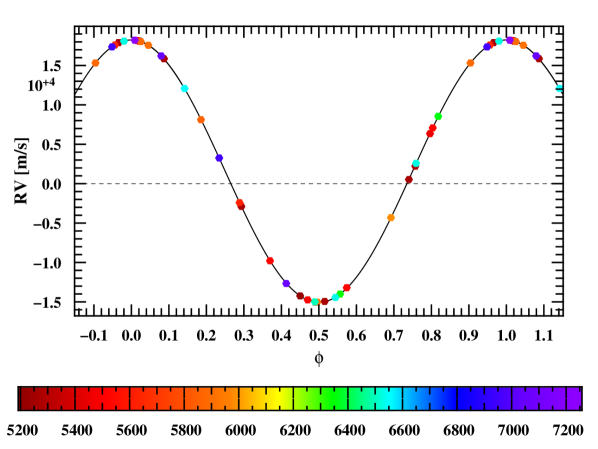
(a) EBLM J0543-57 inner: $m_{\rm B}=0.16M_{\odot}$, $P=4.464$ d, $e=0$

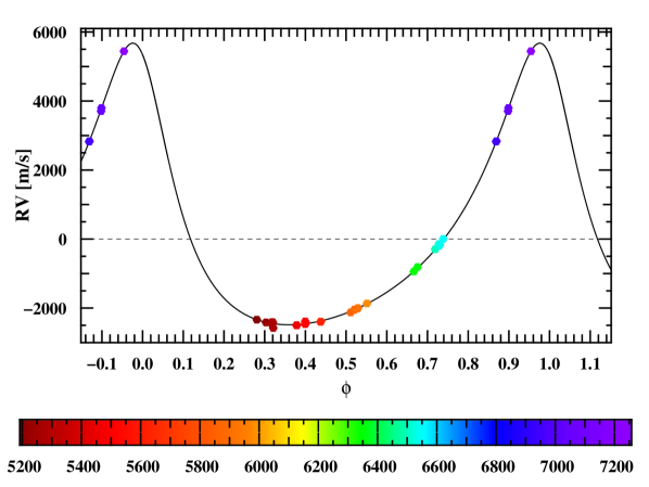
(b) EBLM J0543-57 outer: $m_{\rm C}=0.366M_{\odot}$, $P=3062.039$ d, $e=0.426$

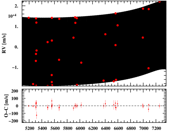
(c) EBLM J0543-57 RVs over time and residuals

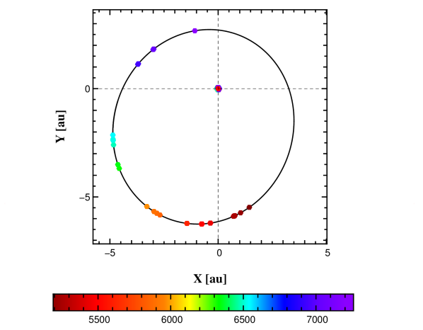
(d) EBLM J0543-57 inner and outer orbit diagrams

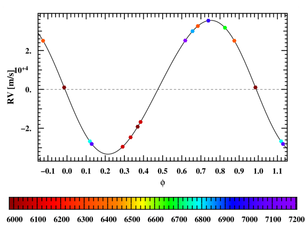
(e) EBLM J1146-42 inner: $m_{\rm B}=0.539M_{\odot}$, $P=10.466$ d, $e=0.06$

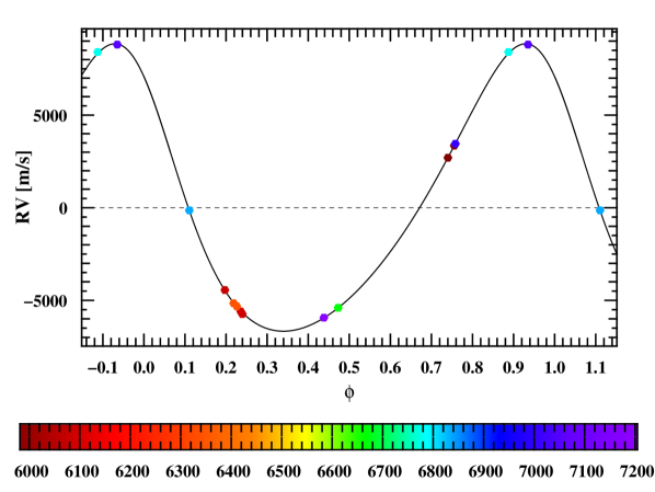
(f) EBLM J1146-42 outer: $m_{\rm C}=0.393M_{\odot}$, $P=259.835$ d, $e=0.219$

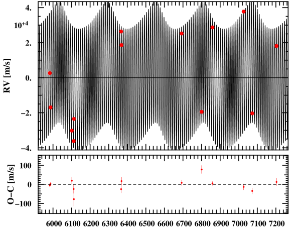
(g) EBLM J1146-42 RVs over time and residuals

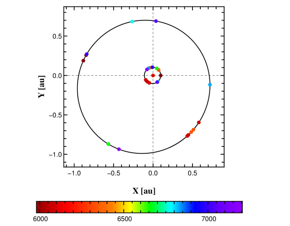
(h) EBLM J1146-42 inner and outer orbit diagrams

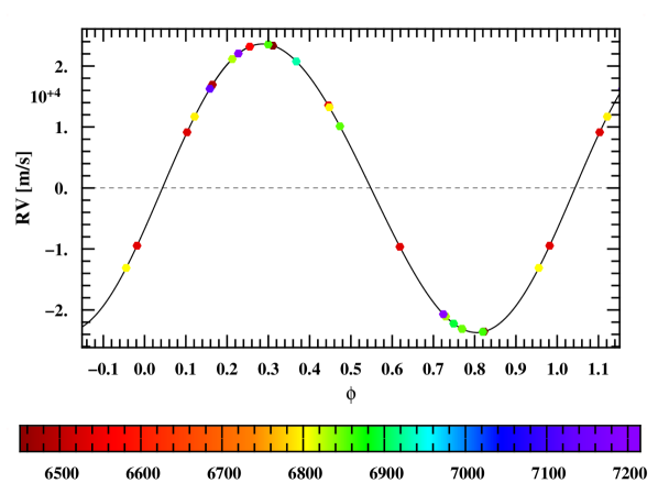
(i) EBLM J2011-71 inner: $m_{\rm B}=0.285M_{\odot}$, $P=5.873$ d, $e=0.031$

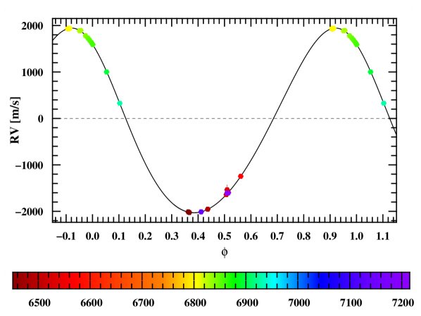
(j) EBLM J2011-71 outer: $m_{\rm C}=0.121M_{\odot}$, $P=662.54$ d, $e=0.101$

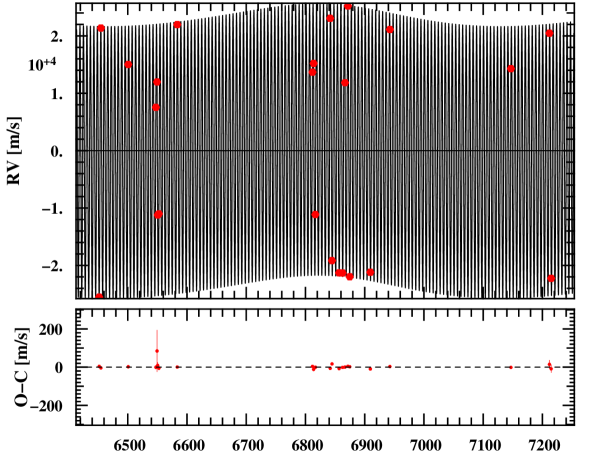
(k) EBLM J2011-71 RVs over time and residuals

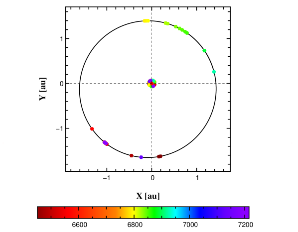
(l) EBLM J2011-71 inner and outer orbit diagrams

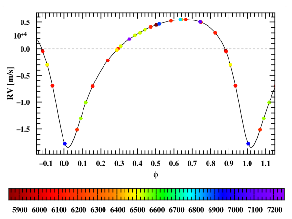
(m) EBLM J2046-40 inner: $m_{\rm B}=0.193M_{\odot}$, $P=37.014$ d, $e=0.473$

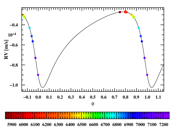
(n) EBLM J2046-40 outer: $m_{\rm C}=0.379M_{\odot}$, $P=5583.664$ d, $e=0.5$

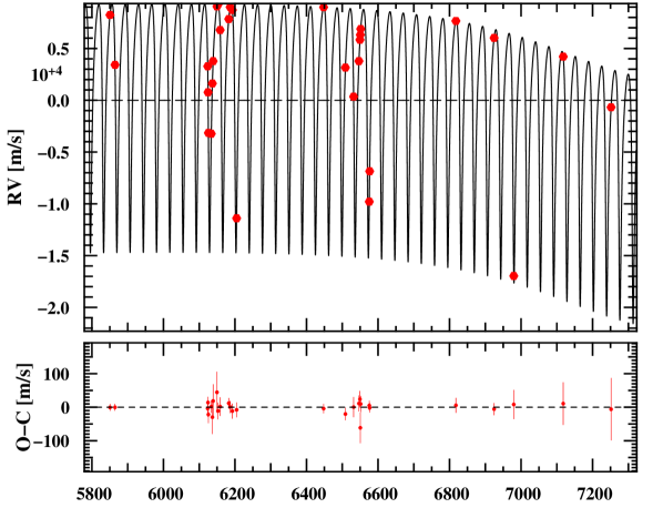
(o) EBLM J2046-40 RVs over time and residuals

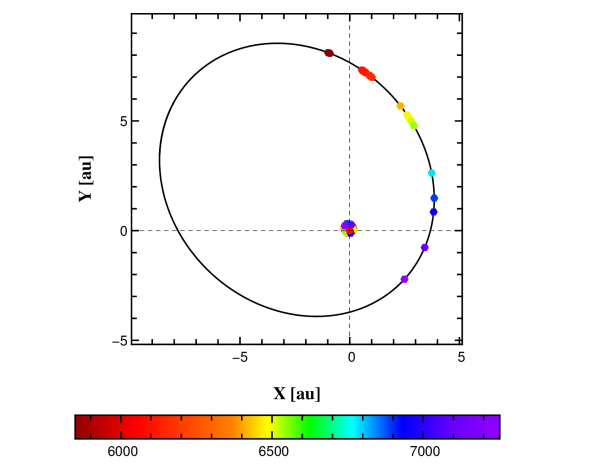
(p) EBLM J2046-40 inner and outer orbit diagrams

References

- Albrecht et al. (2012) Albrecht, S., Winn, J. N., Johnson, J. A., et al. 2012, ApJ, 757, 18
- Albrecht et al. (2014) Albrecht, S., Winn, J. N., Torres, G., et al. 2014, ApJ, 785, 83
- Anderson et al. (2010) Anderson, D. R., Hellier, C., Gillon, M., et al. 2010, ApJ, 709, 159
- Anderson et al. (2016) Anderson, K. R., Lai, D., & Storch, N. I. 2016, ArXiv e-prints
- Bakos et al. (2013) Bakos, G. Á., Csubry, Z., Penev, K., et al. 2013, PASP, 125, 154
- Baraffe et al. (1998) Baraffe, I., Chabrier, G., Allard, F., & Hauschildt, P. H. 1998, A&A, 337, 403
- Baraffe et al. (2015) Baraffe, I., Homeier, D., Allard, F., & Chabrier, G. 2015, A&A, 577, A42
- Baranne et al. (1996) Baranne, A., Queloz, D., Mayor, M., et al. 1996, A&AS, 119, 373
- Bate (2012) Bate, M. R. 2012, MNRAS, 419, 3115
- Bessell (2000) Bessell, M. S. 2000, PASP, 112, 961
- Bessell (2005) Bessell, M. S. 2005, ARA&A, 43, 293
- Bouchy et al. (2016) Bouchy, F., Ségransan, D., Díaz, R. F., et al. 2016, A&A, 585, A46
- Boyajian et al. (2013) Boyajian, T. S., von Braun, K., van Belle, G., et al. 2013, ApJ, 771, 40
- Brogi et al. (2012) Brogi, M., Snellen, I. A. G., de Kok, R. J., et al. 2012, Nature, 486, 502
- Chabrier (2003) Chabrier, G. 2003, PASP, 115, 763
- Chabrier & Baraffe (1997) Chabrier, G. & Baraffe, I. 1997, A&A, 327, 1039
- Chen & Kipping (2016) Chen, J. & Kipping, D. M. 2016, ArXiv e-prints
- Collier Cameron et al. (2007) Collier Cameron, A., Wilson, D. M., West, R. G., et al. 2007, MNRAS, 380, 1230
- Correia et al. (2010) Correia, A. C. M., Couetdic, J., Laskar, J., et al. 2010, A&A, 511, A21
- Cox (2000) Cox, A. N. 2000, Allen’s astrophysical quantities
- Crouzet et al. (2010) Crouzet, N., Guillot, T., Agabi, A., et al. 2010, A&A, 511, A36
- Davenport et al. (2014) Davenport, J. R. A., Ivezić, Ž., Becker, A. C., et al. 2014, MNRAS, 440, 3430
- Dawson (2014) Dawson, R. I. 2014, ApJ, 790, L31
- de Bruijne (2012) de Bruijne, J. H. J. 2012, Ap&SS, 341, 31
- de Wit et al. (2016) de Wit, J., Wakeford, H. R., Gillon, M., et al. 2016, Nature, 537, 69
- Demory et al. (2009) Demory, B.-O., Ségransan, D., Forveille, T., et al. 2009, A&A, 505, 205
- DENIS Consortium (2005) DENIS Consortium. 2005, VizieR Online Data Catalog, 2263, 0
- Díaz et al. (2014) Díaz, R. F., Montagnier, G., Leconte, J., et al. 2014, A&A, 572, A109
- Dotter et al. (2008) Dotter, A., Chaboyer, B., Jevremović, D., et al. 2008, ApJS, 178, 89
- Dumusque et al. (2015) Dumusque, X., Pepe, F., Lovis, C., & Latham, D. W. 2015, ApJ, 808, 171
- Duquennoy & Mayor (1991) Duquennoy, A. & Mayor, M. 1991, A&A, 248, 485
- Esposito et al. (2014) Esposito, M., Covino, E., Mancini, L., et al. 2014, A&A, 564, L13
- Fabrycky & Tremaine (2007) Fabrycky, D. & Tremaine, S. 2007, ApJ, 669, 1298
- Figueira et al. (2013) Figueira, P., Santos, N. C., Pepe, F., Lovis, C., & Nardetto, N. 2013, ArXiv e-prints
- Fiorucci & Munari (2003) Fiorucci, M. & Munari, U. 2003, A&A, 401, 781
- Foreman-Mackey et al. (2013) Foreman-Mackey, D., Hogg, D. W., Lang, D., & Goodman, J. 2013, PASP, 125, 306
- Gaudi et al. (2017) Gaudi, B. S., Stassun, K. G., Collins, K. A., et al. 2017, Nature, 546, 514
- Giacobbe et al. (2012) Giacobbe, P., Damasso, M., Sozzetti, A., et al. 2012, MNRAS, 424, 3101
- Gillon et al. (2013) Gillon, M., Jehin, E., Delrez, L., et al. 2013, in Protostars and Planets VI Posters
- Gillon et al. (2016) Gillon, M., Jehin, E., Lederer, S. M., et al. 2016, Nature, 533, 221
- Gillon et al. (2017) Gillon, M., Triaud, A. H. M. J., Demory, B.-O., et al. 2017, Nature, 542, 456
- Gómez Maqueo Chew et al. (2014) Gómez Maqueo Chew, Y., Morales, J. C., Faedi, F., et al. 2014, A&A, 572, A50
- Gray (2008) Gray, D. F. 2008, The Observation and Analysis of Stellar Photospheres, ed. Gray, D. F.
- Grether & Lineweaver (2006) Grether, D. & Lineweaver, C. H. 2006, ApJ, 640, 1051
- Hale (1994) Hale, A. 1994, AJ, 107, 306
- Hatzes & Rauer (2015) Hatzes, A. P. & Rauer, H. 2015, ApJ, 810, L25
- He et al. (2017) He, M. Y., Triaud, A. H. M. J., & Gillon, M. 2017, MNRAS, 464, 2687
- Henden et al. (2015) Henden, A. A., Levine, S., Terrell, D., & Welch, D. L. 2015, in American Astronomical Society Meeting Abstracts, Vol. 225, American Astronomical Society Meeting Abstracts, 336.16
- Henry et al. (2006) Henry, T. J., Jao, W.-C., Subasavage, J. P., et al. 2006, AJ, 132, 2360
- Høg et al. (2000) Høg, E., Fabricius, C., Makarov, V. V., et al. 2000, A&A, 355, L27
- Howard et al. (2012) Howard, A. W., Marcy, G. W., Bryson, S. T., et al. 2012, ApJS, 201, 15
- Howell et al. (2014) Howell, S. B., Sobeck, C., Haas, M., et al. 2014, PASP, 126, 398
- Hut (1981) Hut, P. 1981, A&A, 99, 126
- Kass & Raftery (1995) Kass, R. E. & Raftery, A. E. 1995, Journal of the American Statistical Association, 90, 773
- Knutson et al. (2014) Knutson, H. A., Fulton, B. J., Montet, B. T., et al. 2014, ApJ, 785, 126
- Kozai (1962) Kozai, Y. 1962, AJ, 67, 579
- Latham et al. (2002) Latham, D. W., Stefanik, R. P., Torres, G., et al. 2002, AJ, 124, 1144
- Lendl et al. (2014) Lendl, M., Triaud, A. H. M. J., Anderson, D. R., et al. 2014, A&A, 568, A81
- Lidov (1962) Lidov, M. L. 1962, Planet. Space Sci., 9, 719
- López-Morales et al. (2014) López-Morales, M., Triaud, A. H. M. J., Rodler, F., et al. 2014, ApJ, 792, L31
- Lovis & Pepe (2007) Lovis, C. & Pepe, F. 2007, A&A, 468, 1115
- Luger et al. (2017) Luger, R., Sestovic, M., Kruse, E., et al. 2017, ArXiv e-prints
- Ma & Ge (2014) Ma, B. & Ge, J. 2014, MNRAS, 439, 2781
- Marcy & Butler (2000) Marcy, G. W. & Butler, R. P. 2000, PASP, 112, 137
- Marmier (2014) Marmier, M. 2014, PhD thesis, Geneva Observatory, University of Geneva
- Marmier et al. (2013) Marmier, M., Ségransan, D., Udry, S., et al. 2013, A&A, 551, A90
- Mathieu et al. (1990) Mathieu, R. D., Latham, D. W., & Griffin, R. F. 1990, AJ, 100, 1859
- Mathieu et al. (2004) Mathieu, R. D., Meibom, S., & Dolan, C. J. 2004, ApJ, 602, L121
- Maxted et al. (2014) Maxted, P. F. L., Bloemen, S., Heber, U., et al. 2014, MNRAS, 437, 1681
- Mayor et al. (2011) Mayor, M., Marmier, M., Lovis, C., et al. 2011, eprint arXiv:1109.2497
- Mayor & Queloz (1995) Mayor, M. & Queloz, D. 1995, Nature, 378, 355
- Mayor et al. (2009) Mayor, M., Udry, S., Lovis, C., et al. 2009, A&A, 493, 639
- Mazeh et al. (1997) Mazeh, T., Mayor, M., & Latham, D. W. 1997, ApJ, 478, 367
- Mazeh & Shaham (1979) Mazeh, T. & Shaham, J. 1979, A&A, 77, 145
- Meibom & Mathieu (2005) Meibom, S. & Mathieu, R. D. 2005, ApJ, 620, 970
- Melo et al. (2001) Melo, C. H. F., Covino, E., Alcalá, J. M., & Torres, G. 2001, A&A, 378, 898
- Milliman et al. (2014) Milliman, K. E., Mathieu, R. D., Geller, A. M., et al. 2014, AJ, 148, 38
- Molaro et al. (2013) Molaro, P., Monaco, L., Barbieri, M., & Zaggia, S. 2013, MNRAS, 429, L79
- Monet et al. (2003) Monet, D. G., Levine, S. E., Canzian, B., et al. 2003, AJ, 125, 984
- Motalebi et al. (2015) Motalebi, F., Udry, S., Gillon, M., et al. 2015, A&A, 584, A72
- Neveu-VanMalle et al. (2016) Neveu-VanMalle, M., Queloz, D., Anderson, D. R., et al. 2016, A&A, 586, A93
- Neveu-VanMalle et al. (2014) Neveu-VanMalle, M., Queloz, D., Anderson, D. R., et al. 2014, A&A, 572, A49
- Nutzman & Charbonneau (2008) Nutzman, P. & Charbonneau, D. 2008, PASP, 120, 317
- Pepe et al. (2002) Pepe, F., Mayor, M., Rupprecht, G., et al. 2002, The Messenger, 110, 9
- Pepper et al. (2012) Pepper, J., Kuhn, R. B., Siverd, R., James, D., & Stassun, K. 2012, PASP, 124, 230
- Pinsonneault et al. (2001) Pinsonneault, M. H., DePoy, D. L., & Coffee, M. 2001, ApJ, 556, L59
- Pollacco et al. (2006) Pollacco, D. L., Skillen, I., Collier Cameron, A., et al. 2006, PASP, 118, 1407
- Queloz et al. (2001a) Queloz, D., Henry, G. W., Sivan, J. P., et al. 2001a, A&A, 379, 279
- Queloz et al. (2001b) Queloz, D., Mayor, M., Udry, S., et al. 2001b, The Messenger, 105, 1
- Rauer et al. (2014) Rauer, H., Catala, C., Aerts, C., et al. 2014, Experimental Astronomy, 38, 249
- Ricker et al. (2014) Ricker, G. R., Winn, J. N., Vanderspek, R., et al. 2014, in Society of Photo-Optical Instrumentation Engineers (SPIE) Conference Series, Vol. 9143, Society of Photo-Optical Instrumentation Engineers (SPIE) Conference Series, 20
- Rodler et al. (2012) Rodler, F., Lopez-Morales, M., & Ribas, I. 2012, ApJ, 753, L25
- Sahlmann et al. (2011) Sahlmann, J., Ségransan, D., Queloz, D., et al. 2011, A&A, 525, A95
- Santerne et al. (2016) Santerne, A., Moutou, C., Tsantaki, M., et al. 2016, A&A, 587, A64
- Santos et al. (2002) Santos, N. C., Mayor, M., Naef, D., et al. 2002, A&A, 392, 215
- Sato et al. (2005) Sato, B., Fischer, D. A., Henry, G. W., et al. 2005, ApJ, 633, 465
- Schlafly & Finkbeiner (2011) Schlafly, E. F. & Finkbeiner, D. P. 2011, ApJ, 737, 103
- Schwarz (1978) Schwarz, G. 1978, Annals of Statistics, 6, 461
- Ségransan et al. (2010) Ségransan, D., Udry, S., Mayor, M., et al. 2010, A&A, 511, A45
- Skrutskie et al. (2006) Skrutskie, M. F., Cutri, R. M., Stiening, R., et al. 2006, AJ, 131, 1163
- Terquem et al. (1998) Terquem, C., Papaloizou, J. C. B., Nelson, R. P., & Lin, D. N. C. 1998, ApJ, 502, 788
- Tokovinin et al. (2006) Tokovinin, A., Thomas, S., Sterzik, M., & Udry, S. 2006, A&A, 450, 681
- Torres et al. (2010) Torres, G., Bakos, G. Á., Hartman, J., et al. 2010, ApJ, 715, 458
- Torres & Ribas (2002) Torres, G. & Ribas, I. 2002, ApJ, 567, 1140
- Triaud (2011) Triaud, A. H. M. J. 2011, PhD thesis, Observatoire Astronomique de l’Universite de Geneve, http://archive-ouverte.unige.ch/unige:18065
- Triaud (2014) Triaud, A. H. M. J. 2014, MNRAS, 439, L61
- Triaud et al. (2010) Triaud, A. H. M. J., Collier Cameron, A., Queloz, D., et al. 2010, A&A, 524, A25
- Triaud et al. (2015) Triaud, A. H. M. J., Gillon, M., Ehrenreich, D., et al. 2015, MNRAS, 450, 2279
- Triaud et al. (2013) Triaud, A. H. M. J., Hebb, L., Anderson, D. R., et al. 2013, A&A, 549, A18
- Triaud et al. (2016) Triaud, A. H. M. J., Neveu-VanMalle, M., Lendl, M., et al. 2016, ArXiv e-prints
- Triaud et al. (2011) Triaud, A. H. M. J., Queloz, D., Hellier, C., et al. 2011, A&A, 531, A24
- Turner et al. (2016) Turner, O. D., Anderson, D. R., Collier Cameron, A., et al. 2016, PASP, 128, 064401
- Udry et al. (2003) Udry, S., Mayor, M., & Santos, N. C. 2003, A&A, 407, 369
- von Boetticher et al. (2017) von Boetticher, A., Triaud, A. H. M. J., Queloz, D., et al. 2017, ArXiv e-prints
- Wheatley et al. (2013) Wheatley, P. J., Pollacco, D. L., Queloz, D., et al. 2013, in European Physical Journal Web of Conferences, Vol. 47, European Physical Journal Web of Conferences, 13002
- Wilson et al. (2008) Wilson, D. M., Gillon, M., Hellier, C., et al. 2008, ApJ, 675, L113
- Winn & Fabrycky (2015) Winn, J. N. & Fabrycky, D. C. 2015, ARA&A, 53, 409
- Zahn (1975) Zahn, J.-P. 1975, A&A, 41, 329
- Zahn (1977) Zahn, J.-P. 1977, A&A, 57, 383
- Zahn & Bouchet (1989) Zahn, J.-P. & Bouchet, L. 1989, A&A, 223, 112
- Zahn (1978) Zahn, J.-R. 1978, A&A, 67, 162