A Loosely-Coupled Approach for Metric Scale Estimation in Monocular Vision-Inertial Systems

Abstract

In monocular vision systems, lack of knowledge about metric distances caused by the inherent scale ambiguity can be a strong limitation for some applications. We offer a method for fusing inertial measurements with monocular odometry or tracking to estimate metric distances in inertial-monocular systems and to increase the rate of pose estimates. As we performed the fusion in a loosely-coupled manner, each input block can be easily replaced with one’s preference, which makes our method quite flexible. We experimented our method using the ORB-SLAM algorithm for the monocular tracking input and Euler forward integration to process the inertial measurements. We chose sets of data recorded on UAVs to design a suitable system for flying robots.

I INTRODUCTION

In recent times, research interest for monocular vision has been strongly increasing in robotics applications. The use of vision-based sensors such as cameras have numerous advantages. They have low energy consumption, they can be manufactured in very small sizes and their cost is dramatically reducing every year. Their typical applications include autonomous navigation, surveillance or mapping. A key issue that directly impacts on the success of these applications is the estimation of locations and distances by using the information gathered by these visual sensors. Several studies show that combining visual information with low-cost, widely available inertial sensors, Inertial Measurement Units (IMUs), improves the accuracy of these estimations.

In this paper, we focus on this kind of sensor sets, called “inertial-monocular” systems, which are composed of a monocular camera and an IMU attached to Unmanned Aerial Vehicles (UAVs). We present a computationally lightweight, and fast solution for estimating the metric distances over the visual information collected by the monocular camera of a UAV. The problem is summarized as follows: By using the frames provided by the camera, algorithms for odometry or Simultaneous Localization And Mapping (SLAM) [1] can estimate the camera positions and orientations (camera poses) and, for the SLAM, create a 3-D representation of the environment. However, the estimates are calculated up to scale [2]. This scale ambiguity is inherent to monocular vision and cannot be avoided. When a 3-D scene is captured by the camera and projected into a 2-D frame, depth information is lost. By measuring the same scene from different points of views, depth can be reconstructed up to scale. The scale factor is different for each frame, nevertheless recent algorithms provide consistent camera pose estimates, which include the estimation of this scale factor. However, the estimation of the scale factor does not provide metric distances. The scale factor is used to ensure consistency in the estimation of camera positions, i.e., large distances in the world coordinate frame measured from a frame $F_{i}$ remain large even if they are measured again from another frame $F_{j}$. To recover metric distances, the length of the camera position vector has to be rescaled using a coefficient. This scaling operation results in metric estimates for distances. The aim of our method is to compute this scaling coefficient.

As mentioned above, monocular vision systems cannot recover the scale of the world; therefore, at least one additional sensor capable of measuring or estimating metric distances must be added to the system. Several sensors can meet this requirement such as lidar, ultrasound or IMU. The use of IMU is often preferred in UAVs because of its small size and low cost. However, IMU does not measure distances directly but acceleration and angular velocities in the inertial frame. Distances can be recovered through the calculation of positions by integrating the acceleration measurements but, consequently, the estimates drift quickly with the error accumulation, which prevents any long-term integration.

The approach we propose is based on distances ($L^{2}$ norm of translation vectors) and is suitable to fuse the output of any monocular odometry or the tracking part of SLAM algorithms with inertial measurements. An overview of the system architecture is shown in Fig. 1. In the following sections, we first provide an overview of the leading approaches. Then, mathematical details of the estimation of scaling coefficient by using IMU measurements are presented. Finally, we test the validity of our method over a set of UAV trajectories [3].

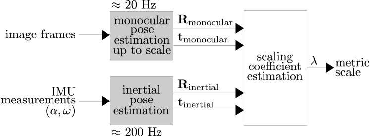
Figure 1: Overview of the system architecture: The blocks in grey can be replaced with one’s preferences. For our experiments, we used the ORB-SLAM algorithm for monocular pose estimation and Euler forward integration for inertial pose estimation.

II RELATED WORKS

Two main approaches for monocular visual-inertial fusion can be distinguished in the literature: Loosely-coupled filtering [4] [5] [6] and tightly-coupled systems [7] [8].

In tightly-coupled approaches, the fusion is done at a low level of the system. Therefore, this requires a deep understanding of the involved algorithms and specific design for the system.

The method described in [8] is the inertial extension of the DPPTAM [9], a direct SLAM algorithm. The tracking thread is modified to include the IMU measurements. The Gauss-Newton optimization is used to minimize the intensity and IMU residuals. The state vector is composed of the position, orientation and velocity of the robot and the IMU biases. The IMU measurements are integrated between two consecutive keyframes. The IMU residuals are the error of the inertial integration between two keyframe with regard to the state value at the corresponding time. The intensity residuals are the photometric error between two keyframes. They are calculated by reprojecting the map points in the keyframes using the estimate of the relative camera pose. The optimization of both residuals provide the final pose estimate of the current keyframe with regard to the world coordinate frame.

The method described in [7] is the inertial extension of ORB-SLAM [10]. In ORB-SLAM, no functionality is provided to calculate the uncertainty of pose estimates. Therefore, the implemented method needs to avoid the direct use of the uncertainty of the camera pose. To represent information about uncertainty, the authors use information matrices computed either from the preintegration of the IMU measurements or from the feature extraction. The reprojection error and inertial error are minimized using the Gauss-Newton optimization. The reprojection error comes from the reprojection of map points in the current keyframe while the IMU error is derived from the preintegration equations described in [11].

In contrast to tightly-coupled approaches, in loosely-coupled approaches, the vision part is considered as a black box, only the output of the box is used. In most loosely-coupled algorithms such as [4] [5] [6], the filter, which fuses the measurements, is derived from Kalman Filtering, e.g., Extended Kalman Filter or Multi-State Constraints Kalman Filter. The state is, at least, composed of the position, orientation, velocity and biases of the IMU. The differential equations, which govern the system and the IMU measurements, are used to predict the state. The incorporation of monocular visual measurements is done through the measurement model when the Kalman gain needs to be computed (the visual measurements update the state when the innovation is calculated).

In [4], the state vector additionally includes the calibration states (the constant relative position and orientation between the IMU coordinate frame and the camera coordinate frame) and a failure detection system. When a failure is detected (abrupt changes in the orientation estimates with regard to the measurement rate), the related visual measurements are automatically discarded to prevent the corruption of data.

In [5], the authors use trifocal tensor geometry which considers epipolar constraints in triples of consecutive images instead of pairs of images. Therefore, in addition to the usual IMU states, the state vector also contains the pose and orientation of the two previous keyframes.

In [6], the fusion is done by using measurements from three sensors: In addition to the visual and inertial sensors, a sonar is included in the system to measure distances (the altitude between the UAV and the ground). IMU is used to detect whether the UAV is flying level or tilted. If it is level, the sonar measurements are directly used to estimate the altitude. Otherwise, IMU measurements help to rectify the incorrect altitude information due to the tilting of the UAV. The scale factor estimation is represented as an optimization problem between the sonar and visual altitude measurements which is solved using the Levenberg-Marquardt algorithm [12].

In this paper, we propose an approach for fusing monocular and inertial measurements in a loosely-coupled manner which is simple to implement, requires small computational resources and so, is suitable for UAVs. We decided to design a loosely-coupled approach to make the methods used for visual tracking and IMU measurement integration easy to replace with any other method ones may prefer, which ensures better flexibility and usability for our approach. In our studies, we used the ORB-SLAM algorithm [10] for the visual tracking part and Euler forward integration for the inertial measurements processing.

III SCALING COEFFICIENT ESTIMATION WITH IMU MEASUREMENTS

III-A Coordinate Frames

Our system (see Fig. 1) is composed of two sensors (a camera and an IMU) attached on a rigid flying body, the UAV. We distinguish four coordinate frames: camera {$C$}, vision {$V$}, inertial {$I$} and world {$W$} coordinate frames. The IMU measures data in {$I$} attached to the body of the UAV. The integration of IMU measurements results in the estimation of the pose of the IMU in {$W$}. The monocular pose estimation algorithm outputs the camera poses in {$V$}, which corresponds to the first {$C$} coordinate frame when the tracking starts, i.e.

$$\{{V}\}\mathrel{\stackon[1.5pt]{=}{\stretchto{\scalerel*[width("=")]{\wedge}{\rule{4.30554pt}{12.91663pt}}}{0.5ex}}}\{{C}\}_{\text{t}=0}$$ (1)

The matrix ${}^{I}\mathbf{T}_{C}$, which represents the transformation between {$C$} and {$I$}, is constant, and can be computed off-line using a calibration method [13]. In the EuRoC dataset sequences that we used for our experiments, ${}^{I}\mathbf{T}_{C}$ is already provided. We consider that {$W$} corresponds to {$I$} at the moment tracking starts, when the {$V$} coordinate frame is generated, so

$$\{{W}\}\mathrel{\stackon[1.5pt]{=}{\stretchto{\scalerel*[width("=")]{\wedge}{\rule{4.30554pt}{12.91663pt}}}{0.5ex}}}\{{I}\}_{\text{t}=0}$$ (2)

In the following paragraphs, we consider that the monocular pose estimation algorithm outputs measurements in the world coordinate frame by applying the formula

$${}^{W}\!\mathbf{p}={}^{I}\mathbf{T}_{C}{}^{V}\!\mathbf{p}$$ (3)

where $\mathbf{p}$ is a 3-D measurement by the monocular pose estimation algorithm.

III-B Integration of IMU Measurements

TABLE I: Mathematical Notation

Notation	Description
{A}	The coordinate frame {A} referred as $A$ in equations.
${}^{A}\mathbf{R}_{B}$	3-by-3 rotation matrix that rotates vectors from {$B$} to {$A$}.
$\mathbf{t}$	3-by-1 translation vector.
$\mathbf{t}^{i}$	Translation vector calculated from inertial measurements.
$\mathbf{t}^{m}$	Translation vector calculated from monocular vision measurements.
$\mathbf{t}^{g}$	Translation vector calculated from ground truth measurements.
${}^{W}{\textbf{t}}_{F_{i},F_{j}}$	Translation vector between the coordinate frames $F_{i}$ and $F_{j}$ written in the world coordinate frame {W}.
${}^{A}\mathbf{T}_{B}$	Transformation matrix that transforms {B} into {A}.
${}^{A}\mathbf{T}_{B_{p}}$	Transformation matrix that transforms {B} at time $p$ into {A}, implies that ${}^{A}\mathbf{T}_{B}$ is changing along time with respect to {$A$}.
$F_{i}$	Camera coordinate frame associated with the image frame $i$.
$\lambda$	Scaling coefficient.
$\mathbf{b}_{a}$, $\mathbf{b}_{\omega}$	IMU biases for the accelerometers and gyroscopes.
$\mathbf{g}$	The gravity vector.
$\mathbf{a}(p)$	3-by-1 vector which contains the accelerometer measurements at time $p$ (one vector component per axis).
$\bm{\upomega}(p)$	3-by-1 vector which contains the gyroscope measurements at time $p$ (one vector component per axis).
$\Delta T$	Time step in seconds.
${}^{A}\mathbf{p}$	3-by-1 vector of a 3-D measurement in {$A$}.

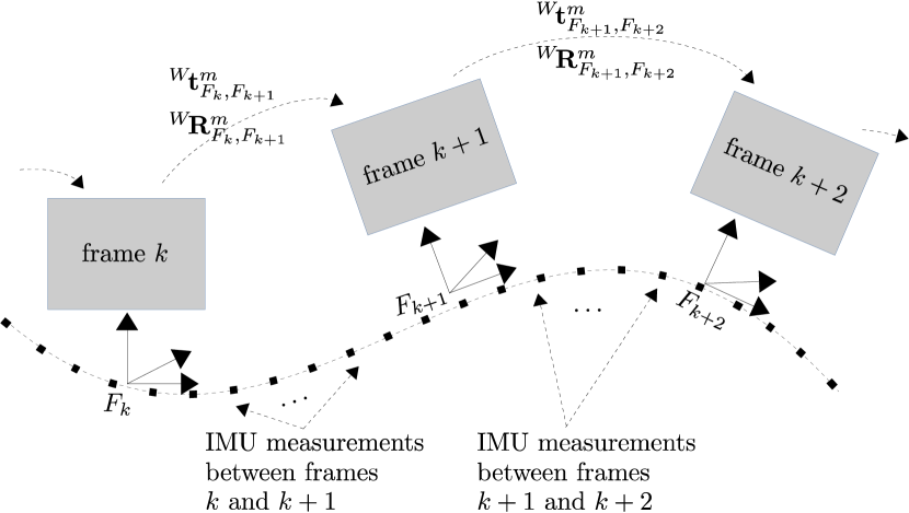
Figure 2: IMU measurements obtained between the two subsequent image frames are used to calculate the translation vectors and rotation matrices.

We assume having a monocular pose estimation algorithm which outputs consistent camera poses in the world coordinate frame. As a monocular camera cannot be used to calculate metric distances, we use the IMU measurements to compute the scaling coefficient. IMU is a sensor composed of three accelerometers and three gyroscopes which respectively measure accelerations and angular velocities along each of the three axis of the inertial frame. The pose of the IMU can be estimated by integrating the accelerometer and gyroscope measurements. However, the integration of the IMU measurement noise and the IMU biases makes the pose estimates to drift fast. Therefore, IMU measurements must be integrated only over a short period for limiting the drift and consequently to corrupt the estimates. We integrate IMU measurements between two consecutive image frames. So, if $F_{k}$ and $F_{k+1}$ are two coordinate frames associated with image frames $k$ and $k+1$ (see Fig. 2), the integration results in the estimation of the rotation matrix ${}^{F_{k}}\textbf{R}_{F_{k+1}}$, velocity ${}^{W}\textbf{v}_{F_{k},F_{k+1}}$ and translation ${}^{W}\textbf{t}_{F_{k},F_{k+1}}$ vectors between the two consecutive frames $F_{k}$ and $F_{k+1}$ in the world coordinate frame using IMU measurements.

We integrated the IMU measurements using Euler forward integration following the description given in [8]

$${}^{F_{i}}\textbf{R}_{F_{j}}=\prod_{p=k}^{k+N-1}\exp_{\text{SO(3)}}([\bm{\upomega}(p)+\mathbf{b}_{\omega}(p)]^{\wedge}\Delta T)$$ (4)

where $\bm{\upomega}$ is the vector of gyroscope measurements, $\mathbf{b}_{\omega}$ the gyroscope bias, $k$ the time step of frame $F_{i}$, $k+N$ the time step of frame $F_{j}$, $N-1$ the number of IMU measurements between the consecutive frames $F_{i}$ and $F_{j}$ and $\Delta T$ is the time step size (in seconds)

$${}^{W}\textbf{v}_{F_{i},F_{j}}=\sum_{p=k}^{k+N-1}[^{W}\mathbf{R}_{I_{p}}(\mathbf{a}(p)+\textbf{b}_{a}(p))-\mathbf{g}]\Delta T$$ (5)

where ${}^{W}\mathbf{R}_{I_{p}}$ is the rotation matrix between the world coordinate frame and the IMU coordinate frame at time $p$, $\mathbf{a}$ is the vector of accelerometer measurements, $\mathbf{b}_{a}$ the accelerometer bias and $g$ the gravity vector

$${}^{W}{\textbf{t}}_{F_{i},F_{j}}= N^{W}\mathbf{v}_{F_{i}}\Delta T+$$ (6)

$$\frac{1}{2}\sum_{p=k}^{k+N-1}\!\!\Big{[}\left(2\left(k+N-1-p\right)+1\right)$$

$$\left({w}^{\mathbf{R}}_{p}\left(\mathbf{a}(p)+\mathbf{b}_{a}(p)\right)-\mathbf{g}\right)\Big{]}\Delta T^{2}$$

The $\exp_{SO(3)}$ operator maps an vector of so(3) to a matrix of SO(3). The wedge operator $.\wedge$ convert a $3\times 1$ vector into an element of so(3), i.e., a skew-symmetric matrix of size $3\times 3$. The IMU biases, $\mathbf{b}_{a}$ and $\mathbf{b}_{\omega}$, were modeled as a random walk process

$$\mathbf{b}_{a}(k+1)=\mathbf{b}_{a}(k)+\Delta T\bm{\upsigma}_{a}^{2}$$ (7)

where $\bm{\upsigma}_{a}^{2}$ is the variance associated to the IMU accelerometers

$$\mathbf{b}_{\omega}(k+1)=\mathbf{b}_{\omega}(k)+\Delta T\bm{\upsigma}_{\omega}^{2}$$ (8)

where $\bm{\upsigma}_{\omega}^{2}$ is the variance associated to the IMU accelerometers

Note that the IMU integration equations (Eqs. 4, 5, 6) can be replaced with another approach for numerical integration (such as [11]) as long as this calculates the translation vector between two consecutive frames in the world coordinate frame {$W$}.

It is assumed that the estimates provided by the monocular pose estimation algorithm $\mathbf{x}^{\text{m}}$ drift slower than the estimates $\mathbf{x}^{\text{i}}$ computed using the IMU measurements, i.e., $\mathbf{x}^{\text{m}}$ is more accurate than $\mathbf{x}^{\text{i}}$. At each incoming frame, we used the value of $\mathbf{x}^{\text{m}}$ to initialize $\mathbf{x}^{\text{i}}$. We observed that a good initialization for the IMU estimates can greatly improve the accuracy of the estimation of the scaling coefficient. However, the initialization of the estimates $\mathbf{x}^{\text{i}}$ is not discussed in this paper and is part of the further improvement we plan to do.

We also benefit from the high measurement rate of the IMU (between 100 Hz and 200 Hz) to provide fast pose estimates. The pose estimates from the vision algorithm $\mathbf{x}_{\text{m}}$ can be updated once per new frame at maximum. Therefore, the camera pose is updated at the frame rate, usually around 30 Hz, which can be too slow for some applications such as control or navigation.

III-C Calculation of Scaling Coefficient

We want to find the scaling coefficient $\lambda$ as follows

$$\|^{W\!}\mathbf{t}^{\text{i}}\|_{2}=\lambda\|^{W\!}\mathbf{t}^{\text{m}}\|_{2}$$ (9)

where ${}^{W\!}\mathbf{t}^{\text{i}}$ are the translation vectors of the camera position given by the integration of IMU measurements in the world coordinate frame, ${}^{W\!}\mathbf{t}^{\text{m}}$ are the translation vectors of the camera position given by the monocular odometry or SLAM algorithm in the world coordinate frame and $\|.\|_{2}$ is the $L^{2}$ norm of a vector.

For each incoming new frame $F_{j}$, the translation of the camera between the consecutive frames $F_{i}$ and $F_{j}$ in the world coordinate frame given by the monocular vision algorithm ${}^{W\!}\mathbf{t}^{\text{m}}_{F_{i},F_{j}}$ is measured. We then integrate the corresponding IMU measurements using the Eq. (1), (2) and (3) to obtain the corresponding translation from the inertial measurements ${}^{W\!}\mathbf{t}^{\text{i}}_{F_{i},F_{j}}$

$$\lambda_{F_{i},F_{j}}=\frac{\|^{W\!}\mathbf{t}^{\text{i}}_{F_{i},F_{j}}\|_{2}}{\|^{W\!}\mathbf{t}^{\text{m}}_{F_{i},F_{j}}\|_{2}}$$ (10)

So Eq. 10 provides an estimated value of the scaling coefficient $\lambda$.

We can measure $\lambda$ for each frame, but the measurement noise on each measurement is significant because both the outputs of the SLAM algorithm and the IMU integration drift. Four methods have been tested to calculate the scaling coefficient $\hat{\lambda}$ using the measurements $\lambda_{F_{i},F_{j}}$. The four methods are: moving average on $\lambda_{F_{i},F_{j}}$ with an additive model for the error, moving average on $\log(\lambda_{F_{i},F_{j}})$ with a multiplicative model for the error, an autoregressive Filter and a Kalman Filter.

The moving averages are calculated over the available measurements at time $t$

$$\hat{\lambda}_{1}=\frac{1}{M}\sum_{k=2}^{M-1}\left(\frac{\|^{W\!}\mathbf{t}^{\text{i}}_{F_{k},F_{k+1}}\|_{2}}{\|^{W\!}\mathbf{t}^{\text{m}}_{F_{k},F_{k+1}}\|_{2}}\right)$$ (11)

where the error model is additive

$$\hat{\lambda}_{2}=\exp\left(\frac{1}{M}\sum_{k=2}^{M-1}\log\left(\frac{\|^{W\!}\mathbf{t}^{\text{i}}_{F_{k},F_{k+1}}\|_{2}}{\|^{W\!}\mathbf{t}^{\text{m}}_{F_{k},F_{k+1}}\|_{2}}\right)\right)$$ (12)

where the error model is multiplicative and $M$ is the number of frames at the considered discrete time $t$. The first frame is skipped because the error on the first IMU measurement is generally large.

We also decided to implement an autoregressive filter (AR) to estimate $\hat{\lambda}$. Moreover, this filter can be used to check whether the measurements are correlated in time. The current value of the filter output $y(i)$ is a weighted linear combination of the $p$ previous outputs ($p$ is the order of the filter) and the current measurement. The weights are computed by solving the Yule-Walker equations

$$y(i)=K+s(i)+\sum_{j=1}^{p}\alpha_{i}y(i-j)$$ (13)

where $y(i)$ is the output of the AR filter at discrete time $i$, $\alpha_{i}$ are the weights calculated with the Yule-Walker equations, $s$ is a zero-mean random variable with

$$s(i)=\lambda(i)-K$$ (14)

$$\lambda(i)=\frac{\|^{W\!}\mathbf{t}^{\text{i}}_{F_{i},F_{i+1}}\|_{2}}{\|^{W\!}\mathbf{t}^{\text{m}}_{F_{i},F_{i+1}}\|_{2}}$$ (15)

The weights $\alpha_{i}$ and bias term $K$ are calculated solving

$$\begin{bmatrix}\mu\\ c_{1}\\ c_{2}\\ \vdots\\ c_{p}\end{bmatrix}=\begin{bmatrix}1&\mu&\mu&\ldots&\mu\\ \mu&c_{0}&c_{1}&\ldots&c_{p-1}&\\ \mu&c_{1}&c_{0}&\ldots&c_{p-2}&\\ \vdots&\vdots&\vdots&\ddots&\vdots&\\ \mu&c_{p-1}&c_{p-2}&\ldots&c_{0}&\\ \end{bmatrix}\begin{bmatrix}K\\ \alpha_{1}\\ \alpha_{2}\\ \vdots\\ \alpha_{p}\end{bmatrix}$$ (16)

where $c_{p}$ is the cross-correlation of the signal $y$ with temporal lag $p$ and $\mu$ is the average of $y$ at time $i$.

The AR filter diverged and it led to poor accuracy for the estimate $\hat{\lambda}$ in all EuRoC sequences. These results show that the measurements are not temporally correlated and do not follow an autoregressive model.

Finally, a Kalman Filter has been implemented to estimate $\hat{\lambda}$. The model is

$$\lambda_{k}=a\lambda_{k-1}+w_{k}$$ (17)

$$z_{k}=h\lambda_{k-1}+v_{k}$$ (18)

where $a=1$ and $h=1$.

The prediction step is done using

$$\hat{\lambda}_{k|k-1}=a\hat{\lambda}_{k-1|k-1}$$ (19)

and the a priori variance $p_{k|k-1}$

$$p_{k|k-1}=a^{2}p_{k-1|k-1}+q$$ (20)

where $q$ is the covariance of the model white noise $w$.

The correction step is calculated as follows

$$k_{k|k}=\frac{hp_{k|k-1}}{h^{2}p_{k|k-1}+r}$$ (21)

where $k$ is the Kalman gain and $r$ is the covariance of the measurement white noise $v$

$$\hat{\lambda}_{k|k}=\hat{\lambda}_{k|k-1}+k_{k|k}(z_{k}-h\hat{\lambda}_{k|k-1})$$ (22)

and the a posteriori variance $p_{k|k}$

$$p_{k|k}=p_{k|k-1}(1-hk_{k|k})$$ (23)

IV EXPERIMENTAL RESULTS

We experimented the proposed method using the sequences from EuRoC dataset [3] and the ORB-SLAM algorithm [10]. The EuRoC dataset provides eleven sequences recorded by an Asctec Firefly hex-rotor helicopter in two different environments, a room equipped with a Vicon motion capture system and a machine hall. We used the frames from one of the front stereo camera (Aptina MT9V034 global shutter, WVGA monochrome, 20 FPS) to emulate monocular vision and the measurements of the MEMS IMU (ADIS16448, angular rate and acceleration, 200 Hz). The ground truth is measured either by the Vicon motion capture system in the sequences recorded in the Vicon room, or by a Leica MS50 laser tracker and scanner in the machine hall environment.

In the following, the sequences referred as V1_01, V1_02 and V1_03 were recorded in the Vicon room with configuration of texture 1; the sequences referred as V2_01, V2_02 and V2_03 were recorded in the Vicon room with configuration of texture 2; the sequences referred as MH01, MH02, MH03, MH04 and MH05 were recorded in the machine hall using the Leica system. Note that the trajectory of the UAV is different in each sequence.

The estimation of the scaling coefficient during the sequence V1_01 is pictured in Figure 3. The value of the scaling coefficient can be compared to a ground truth value, which is computed using a moving average with Vicon (or Leica) measurements ${}^{W\!}\mathbf{t}^{g}$ instead of IMU measurements

$$\lambda^{g}=\frac{1}{M}\sum_{k=1}^{M-1}\left(\frac{\|^{W\!}\mathbf{t}^{g}_{F_{k},F_{k+1}}\|_{2}}{\|^{W\!}\mathbf{t}^{\text{m}}_{F_{k},F_{k+1}}\|_{2}}\right)$$ (24)

The error $e_{\lambda}$ between the ground truth scaling coefficient $\lambda^{g}$ and the coefficient we estimate using inertial measurement $\hat{\lambda}$ is calculated as follows

$$e_{\lambda}=\|\lambda^{g}-\hat{\lambda}\|_{1}$$ (25)

where $\|.\|_{1}$ is the $L^{1}$ norm.

TABLE II: Scaling coefficient and effect on the trajectory

EuRoC	$\hat{\lambda}$			$\lambda^{g}$	$e_{\lambda}$			RMSE (m)			Total distance (m)
Sequence	$\hat{\lambda}_{1}$	$\hat{\lambda}_{2}$	KF		$\hat{\lambda}_{1}$	$\hat{\lambda}_{2}$	KF	$\hat{\lambda}_{1}$	$\hat{\lambda}_{2}$	KF	Ground truth	Best estimate
V1_01	$2.49$	$1.89$	$12.42$	$2.31$	$0.19$	$0.42$	$10.11$	$\textbf{0}.\textbf{22}$	$0.51$	$12.25$	$59.26$	$63.91\rule{0.0pt}{6.63052pt}$
V1_02	$1.80$	$1.41$	$7.57$	$2.35$	$0.55$	$0.94$	$5.22$	$\textbf{0}.\textbf{55}$	$0.95$	$5.25$	$76.58$	$58.74\rule{0.0pt}{6.63052pt}$
V1_03	$2.55$	$1.92$	$6.73$	$3.54$	$1.00$	$1.63$	$3.19$	$\textbf{0}.\textbf{46}$	$0.75$	$1.47$	$77.53$	$55.78\rule{0.0pt}{6.63052pt}$
V2_01	$2.92$	$2.33$	$1.17$	$3.02$	$0.10$	$0.70$	$1.86$	$\textbf{0}.\textbf{09}$	$0.60$	$1.67$	$36.93$	$35.66\rule{0.0pt}{6.63052pt}$
V2_02	$4.32$	$1.87$	$82.15$	$3.56$	$0.77$	$1.684$	$78.80$	$\textbf{0}.\textbf{47}$	$1.03$	$47.99$	$83.92$	$101.93\rule{0.0pt}{6.63052pt}$
V2_03	$1.94$	$1.42$	$1.26$	$2.15$	$1.84$	$2.36$	$2.52$	$\textbf{1}.\textbf{66}$	$2.13$	$2.27$	$139.15$	$71.30\rule{0.0pt}{6.63052pt}$
MH01	$251.58$	$7.57$	$10.10$	$6.92$	$208.66$	$0.65$	$3.18$	$216.55$	$\textbf{0}.\textbf{68}$	$3.30$	$85.50$	$93.54\rule{0.0pt}{6.63052pt}$
MH02	$51.91$	$2.64$	$1.08$	$2.94$	$48.97$	$0.30$	$1.86$	$146.69$	$\textbf{0}.\textbf{90}$	$5.56$	$84.39$	$75.88\rule{0.0pt}{6.63052pt}$
MH03	$35.81$	$2.31$	$4.93$	$3.77$	$32.04$	$1.46$	$1.16$	$39.85$	$1.82$	$\textbf{1}.\textbf{45}$	$131.13$	$171.45\rule{0.0pt}{6.63052pt}$
MH04	$36.74$	$3.78$	$9.28$	$7.51$	$29.23$	$3.74$	$1.17$	$32.78$	$4.19$	$\textbf{1}.\textbf{98}$	$103.58$	$127.94\rule{0.0pt}{6.63052pt}$
MH05	$33.21$	$2.05$	$2.27$	$2.74$	$30.47$	$0.69$	$0.47$	$109.16$	$2.48$	$\textbf{1}.\textbf{68}$	$116.02$	$96.22\rule{0.0pt}{6.63052pt}$

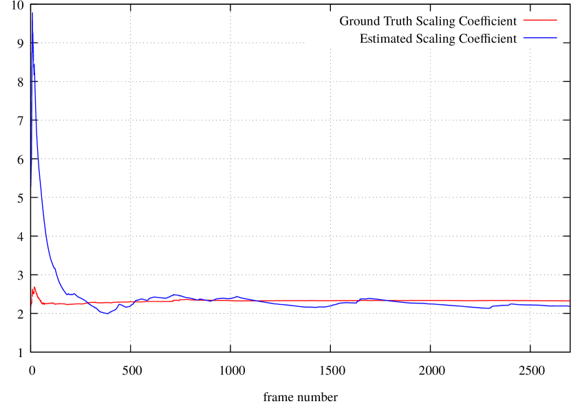
Figure 3: The estimation of the scaling coefficient $\lambda$ using the sequence V1_01 from EuRoC dataset (In blue the ground truth calculated from the Vicon estimates, in red the proposed estimation method).

We rescaled the trajectory provided by the monocular algorithm. As presented in Fig. 4, the distances given by the monocular algorithm are arbitrary but consistent, therefore the UAV’s trajectory is scaled differently than the ground truth. In Fig. 5, we rescaled the monocular trajectory of the sequence V1_01 using the ground truth $\lambda^{g}$ and estimated $\hat{\lambda}_{1}$ scaling coefficients. We computed the root-mean-square deviation (RMSE) for each sequence as follows

$$\text{RMSE}=\sqrt{\frac{\sum_{i=1}^{M}\left(\lambda^{g}\mathbf{x}_{i}^{T}-\hat{\lambda}\mathbf{x}_{i}^{T}\right)\left(\lambda^{g}\mathbf{x}_{i}-\hat{\lambda}\mathbf{x}_{i}\right)}{M}}$$ (26)

where $M$ is the number of frames in the sequence and $\mathbf{x}$ is the position of the camera in the world coordinate given by the monocular algorithm (ORB-SLAM for our experiments). The RMSE for each EuRoC sequence is given in Tab. II.

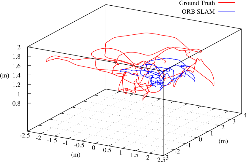
Figure 4: The trajectory of the camera during the V1_01 sequence from EuRoC dataset in the world coordinate frame (ORB-SLAM measurements are in blue, the ground truth measured with a Vicon motion capture system are in red).

The initial trajectory of the UAVs in the sequence V1_01 provided by the ORB-SLAM algorithm is displayed in Fig. 4. The same trajectory rescaled using the scaling coefficients $\lambda^{g}$ and $\hat{\lambda}_{1}$ is displayed in Fig. 5.

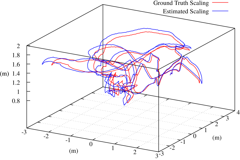
Figure 5: The rescaled trajectory of the camera provided by ORB-SLAM in the V1_01 sequence from EuRoC dataset in the world coordinate frame (the blue trajectory was rescaled using the value of $\lambda$, the red trajectory was rescaled using the ground truth scaling coefficient).

As expected, the bigger the scaling coefficient error $e_{\lambda}$, the bigger the RMSE. The sequences recorded in the Vicon room provide trajectories with lower RMSE than the sequences recorded in the machine hall. The difference between the two sets of sequences can be explained by the strong excitation of the IMU for the calibration of the Leica laser that incorporates a lot of noise in the measurements $\mathbf{t}^{i}$. In the Vicon sequences, the estimate $\hat{\lambda}_{1}$ outperforms. The sequences recorded in the machine hall are very challenging for the inertial fusion because the UAV performed very fast translational movements during a few seconds for Leica ground truth calibration purposes which result in large acceleration measurements and partially corrupt the inertial estimates as shown in Fig. 6. Therefore, in the machine hall sequences where strong noise corrupts some IMU measurements, $\hat{\lambda}_{2}$ is far better than $\hat{\lambda}_{1}$, which never managed to completely absorb the strong perturbations of the calibration. Interestingly, Kalman Filter (KF) gives also satisfactory results for Leica sequences. The results of Kalman Filter can be further improved with a finer tuning of the process noise variance $q$. For instance, with a smaller value for $q$, the RMSE of sequences MH_03 and MH_04 drops to 0.17 m and 0.76 m respectively. As every single EuRoC sequence is quite different from the others, finding a nice tuning value for the Kalman Filter is not straightforward. We recommend to tune the filter accordingly to the type of flight the UAV performs (smoothness and aggressiveness of trajectories, motion speed, angular velocities). If a Kalman Filter cannot be implemented or tuned, $\hat{\lambda}_{2}$ remains a acceptable estimate. More broadly, keeping the IMU out from large perturbations by using smooth trajectories provides more accurate estimates. The estimates computed through the AR filter, which are not presented because of the dramatically large value of RMSE, show that there is no temporal correlation of the error.

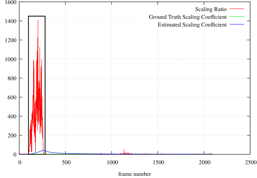
Figure 6: An example of the corruption of estimates due to the fast translational movements (shown in the rectangular area as marked) for the Leica calibration in one of the sequences recorded in the machine hall environment (MH05).

V Concluding Remarks and Future Work

We presented a fast and easy-to-implement method for the calculation of the scaling coefficient by fusing inertial measurements with monocular pose estimation. Monocular camera systems, due to their nature, can not provide the real-world scale of the pose estimates. To overcome this problem, we use the inertial measurements produced by an IMU to i) estimate the scaling coefficient, which relates the monocular camera pose estimation to the real-world scale, and ii) speed up the pose estimation by exploiting the availability of the inertial measurements in very high rates.

The method is highly modular, which makes each component to be easily replaceable with one’s preferences without impacting the overall operation of the system.

To improve the current method, we plan to further investigate the initialization of the IMU integration process, particularly with the incorporation of the current estimate of the scaling coefficient when appropriate.

We defined three approaches for calculating the scaling coefficient with regard to the nature of the trajectory followed by the UAV. We found that the Kalman Filter approach gives accurate estimates when the tuning is done well, which unfortunately can be hard to do for some applications. Determination of the tuning value of the process noise is a complex topic which will be part of our future research work and experimentations.

References

- [1] C. Cadena, L. Carlone, H. Carrillo, Y. Latif, D. Scaramuzza, J. Neira, I. Reid, and J. J. Leonard, “Past, Present, and Future of Simultaneous Localization and Mapping: Towards the Robust-Perception Age,” IEEE Transactions on Robotics, vol. 32, no. 6, pp. 1309–1332, 2016.
- [2] R. Hartley and A. Zisserman, Multiple View Geometry in Computer Vision. Cambridge university press, 2003.
- [3] M. Burri, J. Nikolic, P. Gohl, T. Schneider, J. Rehder, S. Omari, M. W. Achtelik, and R. Siegwart, “The EuRoC Micro Aerial Vehicle Datasets,” The International Journal of Robotics Research, vol. 35 (10), pp. 1157–1163, 2016.
- [4] S. Weiss and R. Siegwart, “Real-Time Metric State Estimation for Modular Vision-Inertial Systems,” in 2011 IEEE International Conference on Robotics and Automation (ICRA), Shanghai, China, 2011, pp. 4531–4537.
- [5] J. S. Hu and M. Y. Chen, “A Sliding-Window Visual-IMU Odometer Based on Tri-Focal Tensor Geometry,” in IEEE International Conference on Robotics and Automation (ICRA), Hong Kong, China, 2014, pp. 3963–3968.
- [6] I. Sa, H. He, V. Huynh, and P. Corke, “Monocular Vision based Autonomous Navigation for a Cost-Effective Open-Source MAVs in GPS-denied Environments,” in 2013 IEEE/ASME International Conference on Advanced Intelligent Mechatronics (AIM), Wollongong, Australia, 2013, pp. 1355–1360.
- [7] R. Mur-Artal and J. D. Tardós, “Visual-Inertial Monocular SLAM with Map Reuse,” IEEE Robotics and Automation Letters, vol. 2, no. 2, pp. 796–803, 2017.
- [8] A. Concha, G. Loianno, V. Kumar, and J. Civera, “Visual-Inertial Direct SLAM,” in IEEE International Conference on Robotics and Automation (ICRA), Stockholm, Sweden, 2016, pp. 1331–1338.
- [9] A. Concha and J. Civera, “DPPTAM: Dense Piecewise Planar Tracking and Mapping from a Monocular Sequence,” in IEEE/RSJ International Conference on Intelligent Robots and Systems (IROS), Hamburg, Germany, 2015, pp. 5686–5693.
- [10] R. Mur-Artal, J. M. M. Montiel, and J. D. Tardos, “ORB-SLAM: A Versatile and Accurate Monocular SLAM System,” IEEE Transactions on Robotics, vol. 31, no. 5, pp. 1147–1163, 2015.
- [11] C. Forster, L. Carlone, F. Dellaert, and D. Scaramuzza, “IMU Preintegration on Manifold for Efficient Visual-Inertial Maximum-a-Posteriori Estimation,” in Robotics: Science and Systems (RSS), Rome, Italy, 2015.
- [12] J. J. Moré, “The Levenberg-Marquardt Algorithm: Implementation and Theory,” in Numerical Analysis. Springer, 1978, pp. 105–116.
- [13] F. M. Mirzaei and S. I. Roumeliotis, “A Kalman Filter-Based Algorithm for IMU-Camera Calibration: Observability Analysis and Performance Evaluation,” IEEE Transactions on Robotics, vol. 24, no. 5, pp. 1143–1156, Oct 2008.