Magnonic topological insulators in antiferromagnets

Abstract

Extending the notion of symmetry protected topological phases to insulating antiferromagnets (AFs) described in terms of opposite magnetic dipole moments associated with the magnetic N$\acute{{\rm{e}}}$el order, we establish a bosonic counterpart of topological insulators in semiconductors. Making use of the Aharonov-Casher effect, induced by electric field gradients, we propose a magnonic analog of the quantum spin Hall effect (magnonic QSHE) for edge states that carry helical magnons. We show that such up and down magnons form the same Landau levels and perform cyclotron motion with the same frequency but propagate in opposite direction. The insulating AF becomes characterized by a topological ${\mathbb{Z}}_{2}$ number consisting of the Chern integer associated with each helical magnon edge state. Focusing on the topological Hall phase for magnons, we study bulk magnon effects such as magnonic spin, thermal, Nernst, and Ettinghausen effects, as well as the thermomagnetic properties of helical magnon transport both in topologically trivial and nontrivial bulk AFs and establish the magnonic Wiedemann-Franz law. We show that our predictions are within experimental reach with current device and measurement techniques.

I Introduction

Since the observation of quasiequilibrium Bose-Einstein condensation Demokritov et al. (2006) of magnons in an insulating ferromagnet (FM) at room temperature, the last decade has seen remarkable and rapid development of a new branch of magnetism, dubbed magnonics Chumak et al. (2015); Serga et al. (2010); Nakata et al. (2017a), aimed at utilizing magnons, the quantized version of spin-waves, as substitute for electrons with the advantage of low-dissipation. Magnons are chargeless bosonic quasi-particles with a magnetic dipole moment $g\mu_{\rm{B}}{\mathbf{e}}_{z}$ that can serve as a carrier of information in units of the Bohr magneton $\mu_{\rm{B}}$. In particular, insulating FMs Kajiwara et al. (2010); Onose et al. (2010); Cornelissen et al. (2015); Liu et al. (2017) that possess a macroscopic magnetization [Fig. 1 (a)] have been playing an essential role in magnonics. Spin-wave spin current Kajiwara et al. (2010); Cornelissen et al. (2015), thermal Hall effect of magnons Onose et al. (2010), and Snell’s law Tanabe et al. (2014); Stigloher et al. (2016) for spin-waves have been experimentally established and just this year the magnon planar Hall effect Liu et al. (2017) has been observed. A magnetic dipole moving in an electric field acquires a geometric phase by the Aharonov-Casher Aharonov and Casher (1984); Mignani (1991); Meier and Loss (2003); Nakata et al. (2014); Ericsson and Sj$\ddot{\rm{o}}$qvist (2001); Liu and Vignale (2011, 2012) (AC) effect, which is analogous to the Aharonov-Bohm effect Aharonov and Bohm (1959); Loss et al. (1990); Loss and Goldbart (1992) of electrically charged particles in magnetic fields, and the AC effect in magnetic systems has also been experimentally confirmed Zhang et al. (2014).

Figure 1: (Color online) Left: Schematic representation of spin excitations in (a) a FM with the uniform ground state magnetization and (b) an AF with classical magnetic N$\acute{{\rm{e}}}$el order. Right: Schematic representation of edge magnon states in a two-dimensional topological (a) FM and (b) AF. (a) Chiral edge magnon state where magnons with a magnetic dipole moment $g\mu_{\rm{B}}{\bf e}_{z}$ propagate along the edge of a finite sample in a given direction. (b) Helical edge magnon state where up and down magnons ($\sigma=\pm 1$) with opposite magnetic dipole moments $\sigma g\mu_{\rm{B}}{\bf e}_{z}$ propagate along the edge in opposite directions. The AF thus forms a bosonic analog of a TI characterized by two edge modes with opposite chiralities and can be identified with two independent copies (with opposite magnetic moments) of single-layer FMs shown in (a).

Under a strong magnetic field, two-dimensional electronic systems can exhibit the integer quantum Hall effect v. Klitzing et al. (1980) (QHE), which is characterized by chiral edge modes. Thouless, Kohmoto, den Nijs, and Nightingale Thouless et al. (1982); Kohmoto (1985) (TKNN) described the QHE  Pankratov (1987); Haldane (1988); Volovik and Yakovenko (1989); Klinovaja et al. (2015) in terms of a topological invariant, known as TKNN integer, associated with bulk wave functions Halperin (1982); Hatsugai (1993) in momentum space. This introduced the notion of topological phases of matter, which has been attracting much attention over the last decade. In particular, in 2005, Kane and Mele Kane and Mele (2005a, b) have shown that graphene in the absence of a magnetic field exhibits a quantum spin Hall effect (QSHE) Kane and Mele (2005b); Bernevig and Zhang (2006); Hasan and Kane (2010); Qi and Zhang (2011), which is characterized by a pair of gapless spin-polarized edge states. These helical edge states are protected from backscattering by time-reversal symmetry (TRS), forming in this sense topologically protected Kramers pairs. This can be seen to be the first example of a symmetry protected topological (SPT) phase Zeng et al. ; Senthil (2015); Senthil and Levin (2013) and it is now classified as a topological insulator (TI) Kane and Mele (2005a); Sheng et al. (2005); Murakami (2006); Hasan and Kane (2010); Qi and Zhang (2011), which is characterized by a ${\mathbb{Z}}_{2}$ number, as the TKNN integer Thouless et al. (1982); Kohmoto (1985) associated with each edge state.

In this paper we extend the notion of topological phases to insulating antiferromagnets (AFs) in the N$\acute{{\rm{e}}}$el ordered phases which do not possess a macroscopic magnetization, see Fig. 1 (b). The component of the total spin along the N$\acute{{\rm{e}}}$el vector is assumed to be conserved, and it is this conservation law which plays the role of the TRS (which is broken in the ordered AF) that protects the topological phase and helical edge states against nonmagnetic impurities and the details of the surface. T. Wolfram and R. E. De Wames (1952) In particular, using magnons Anderson (1952); Kubo (1952); Jungwirth et al. (2016); Gomonaya and Loktev (2014) we thus establish a bosonic counterpart of the TI and propose a magnonic QSHE resulting from the N$\acute{{\rm{e}}}$el order in AFs.

In Ref. [Nakata et al., 2017b], motivated by the above-mentioned remarkable progress in recent experiments, we Meier and Loss (2003); Nakata et al. (2015, 2017a); van Hoogdalem et al. (2013) have proposed a way to electromagnetically realize the ‘quantum’ Hall effect of magnons in FMs, in the sense that the magnon Hall conductances are characterized by a Chern number Thouless et al. (1982); Kohmoto (1985) in an almost flat magnon band, which hosts a chiral edge magnon state, see Fig. 1 (a). By providing a topological description Xiao et al. (2010a); Kohmoto (1985); Thouless et al. (1982) of the classical magnon Hall effect induced by the AC effect, which was proposed in Ref. [Meier and Loss, 2003], we developed it further into the magnonic ‘quantum’ Hall effect and appropriately defining the thermal conductance for bosons, we found that the magnon Hall conductances in such topological FMs obey a Wiedemann-Franz Franz and Wiedemann (1853) (WF) law for magnon transport Nakata et al. (2015, 2017a). In this paper, motivated by the recent experimental Seki et al. (2015) demonstration of thermal generation of spin currents in AFs using the spin Seebeck effect Uchida et al. (2010); Saitoh et al. (2006); Ohnuma et al. (2013); Adachi et al. (2011, 2010); Xiao et al. (2010b); Dejene et al. (2014); Flipse et al. (2014) and by the report Cheng et al. (2016); Zyuzin and Kovalev (2016); Shiomi et al. of the magnonic spin Nernst effect in AFs, we develop Ref. [Nakata et al., 2017b] further into the AF regime Jungwirth et al. (2016); Gomonaya and Loktev (2014); Kubo (1952); Anderson (1952); van Hoogdalem and Loss (2011); Normand et al. (2000) and propose a magnonic analog of the QSHE Kane and Mele (2005b); Bernevig and Zhang (2006); Kane and Mele (2005a); Sheng et al. (2005); Murakami (2006); Hasan and Kane (2010); Qi and Zhang (2011) for edge states that carry helical edge magnons [Fig. 1 (b)] due to the AC phase. Focusing on helical magnon transport both in topologically trivial and nontrivial bulk Halperin (1982); Hatsugai (1993) AFs, we also study thermomagnetic properties and discuss the universality of the magnonic WF law Nakata et al. (2015, 2017b, 2017a). Using magnons in insulating AFs characterized by the N$\acute{{\rm{e}}}$el magnetic order, we thus establish the bosonic counterpart of TIs Kane and Mele (2005a); Sheng et al. (2005); Murakami (2006); Hasan and Kane (2010); Qi and Zhang (2011).

At sufficiently low temperatures, effects of magnon-magnon and magnon-phonon interactions become Nakata et al. (2015); Adachi et al. (2010); Prasai et al. (2017) negligibly small. Indeed, Ref. [Prasai et al., 2017] reported measurements of magnets at low temperature $T\lesssim{\cal{O}}(1)$K, where the exponent of the temperature dependence of the phonon thermal conductance is larger than the one for magnons. This indicates that for thermal transport the contribution of phonons dies out more quickly than that of magnons with decreasing temperature. We then focus on noninteracting magnons at such low temperatures throughout this work and assume that the total spin along the $z$ direction is conserved and thus remains a good quantum number.

This paper is organized as follows. In Sec. II we introduce the model system for magnons with a quadratic dispersion because of an easy-axis spin anisotropy in a topologically trivial bulk AF and find that the dynamics can be described as the combination of two independent copies of that in a FM and thus derive the identical magnonic WF law for a topologically trivial FM and AF. In Sec. III.1, introducing the model system for magnons in the presence of an AC phase induced by an electric field gradient, we find the correspondence between the single magnon Hamiltonian and the one of an electrically charged particle moving in a magnetic vector potential, and see that the force acting on magnons is invariant under a gauge transformation. In Sec. III.2, we see that each magnon with opposite magnetic dipole moment inherent to the N$\acute{{\rm{e}}}$el order forms the same Landau levels and performs cyclotron motion with the same frequency but in opposite direction, leading to the helical edge magnon state. We find that the AF in the topological ${\mathbb{Z}}_{2}$ phase is characterized by a Chern number associated with each edge state. In Sec. III.3, introducing a tight-binding representation (TBR) of the magnon Hamiltonian, we obtain the magnon energy spectrum and helical edge states numerically, for constant and periodic electric field gradients. In Sec. III.4, we study thermomagnetic properties of Hall transport of bulk magnons, with focus on the the helical edge magnon states, and analyze the differences between the topological and non-topological phases of the AF. In Sec. IV we give some concrete estimates for experimental candidate materials. Finally, we summarize and give some conclusions in Sec. V, and remark open issues in Sec. VI. Technical details are deferred to the Appendices.

II Topologically trivial AF

In this section, we consider a topologically trivial AF on a three-dimensional ($d=3$) cubic lattice in the ordered phase with the N$\acute{{\rm{e}}}$el order parameter along the $z$ direction, see Fig. 1 (b). Spins of length $S$ on each bipartite sublattice, denoted by A and B, satisfy Altland and Simons (2006); Cheng et al. (2016); Zyuzin and Kovalev (2016) ${\mathbf{S}}_{\rm{A}}=-{\mathbf{S}}_{\rm{B}}=S{\mathbf{e}}_{z}$ in the ground state. The magnet is described by the following spin Hamiltonian, Kubo (1952); Anderson (1952)

$${\cal{H}}=J\sum_{\langle ij\rangle}{\mathbf{S}}_{i}\cdot{\mathbf{S}}_{j}-\frac{\cal{K}}{2}\sum_{i}(S_{i}^{z})^{2},$$ (1)

where $J>0$ parametrizes the antiferromagnetic exchange interaction between the nearest-neighbor spins and ${\cal{K}}>0$ is the easy-axis anisotropy Artman et al. (1965); Kota and Imamura (2017) that ensures the magnetic N$\acute{{\rm{e}}}$el order along the $z$ direction. Since the Hamiltonian is invariant under global spin rotations about the $z$ axis, the $z$ component of the total spin is a good quantum number (i.e. conserved). Therefore, magnons, quanta of spin waves, have well-defined spin along the $z$ axis, as will be shown explicitly below. Using the sublattice-dependent Holstein-Primakoff Holstein and Primakoff (1940); Altland and Simons (2006); Cheng et al. (2016); Zyuzin and Kovalev (2016) transformation, $S_{i{\rm{A}}}^{+}=\sqrt{2S}[1-a_{i}^{\dagger}a_{i}/(2S)]^{1/2}a_{i}$, $S_{i{\rm{A}}}^{z}=S-a_{i}^{\dagger}a_{i}$, $S_{j{\rm{B}}}^{+}=\sqrt{2S}[1-b_{j}^{\dagger}b_{j}/(2S)]^{1/2}b_{j}^{\dagger}$, $S_{j{\rm{B}}}^{z}=-S+b_{j}^{\dagger}b_{j}$, the spin degrees of freedom in Eq. (1) can be recast in terms of bosonic operators that satisfy the commutation relations, $[a_{i},a_{j}^{\dagger}]=\delta_{i,j}$ and $[b_{i},b_{j}^{\dagger}]=\delta_{i,j}$ and all other commutators between the annihilation (creation) operators $a_{i}^{(\dagger)}$ and $b_{i}^{(\dagger)}$ vanish to the lowest order in $1/S$, assuming large spins $S\gg 1$. Further performing the well-known Bogoliubov transformation Altland and Simons (2006) (see Appendix A for details), the system can be mapped onto a system of non-interacting spin-up and spin-down magnons, which carry opposite magnetic dipole moment Altland and Simons (2006) $\sigma g\mu_{\rm{B}}{\bf e}_{z}$ with $\sigma=\pm 1$. The transformed Hamiltonian assumes diagonal form Kubo (1952); Anderson (1952), ${\cal{H}}=\sum_{\mathbf{k}}\hbar\omega_{\mathbf{k}}({\cal{A}}_{\mathbf{k}}^{\dagger}{\cal{A}}_{\mathbf{k}}+{\cal{B}}_{\mathbf{k}}^{\dagger}{\cal{B}}_{\mathbf{k}})$, in terms of Bogoliubov quasi-particle operators, ${\cal{A}}_{\mathbf{k}}$ and ${\cal{B}}_{\mathbf{k}}$, satisfying $[{\cal{A}}_{\mathbf{k}},{\cal{A}}_{{\mathbf{k^{\prime}}}}^{\dagger}]=\delta_{{\mathbf{k}},{\mathbf{k^{\prime}}}}$ and $[{\cal{B}}_{\mathbf{k}},{\cal{B}}_{{\mathbf{k^{\prime}}}}^{\dagger}]=\delta_{{\mathbf{k}},{\mathbf{k^{\prime}}}}$ with all the other commutators vanishing. Within the long wave-length approximation and assuming a spin anisotropy Artman et al. (1965); Kota and Imamura (2017) at low temperature, the dispersion Kubo (1952) becomes gapped and parabolic in terms of $k=|{\mathbf{k}}|$, $\hbar\omega_{{\mathbf{k}}}=Dk^{2}+\Delta$, where $D=JSa^{2}/\sqrt{\kappa^{2}+2\kappa}$ parametrizes the inverse of the ‘magnon mass’ (see below), $\Delta=2dJS\sqrt{\kappa^{2}+2\kappa}$ is the magnon gap, $\kappa={\cal{K}}/(2dJ)$, $a$ denotes the lattice constant, and $d=3$ is the dimension of the cubic lattice (e.g., $d=2$ for the square lattice). Note that the dispersion becomes linear $\hbar\omega_{{\mathbf{k}}}\propto k$ in the absence of the spin anisotropy Anderson (1952), see Appendix A for details.

Since the $z$ component of the total spin is given by Cheng et al. (2016) $S^{z}=\sum_{i}(S_{i{\rm{A}}}^{z}+S_{i{\rm{B}}}^{z})=\sum_{\mathbf{k}}(-a_{\mathbf{k}}^{\dagger}a_{\mathbf{k}}+b_{\mathbf{k}}^{\dagger}b_{\mathbf{k}})=\sum_{\mathbf{k}}(-{\cal{A}}_{\mathbf{k}}^{\dagger}{\cal{A}}_{\mathbf{k}}+{\cal{B}}_{\mathbf{k}}^{\dagger}{\cal{B}}_{\mathbf{k}})$, the ${\cal{A}}$ (${\cal{B}}$) magnon carries $\sigma=-1$ ($+1$) spin angular momentum along the $z$ direction and can be identified with a down (up) magnon. Thus the low-energy magnetic excitation of the AF [Eq. (1)] can be described as chargeless bosonic quasiparticles carrying a magnetic dipole moment $\sigma g\mu_{\rm{B}}{\bf e}_{z}$ with $\sigma=\pm 1$ [Fig. 1 (b)], where $g$ is the $g$-factor of the constituent spins and $\mu_{\rm{B}}$ is the Bohr magneton. Throughout this paper, we work under the assumption that the total spin along the $z$ direction is conserved and remains a good quantum number.

In the presence of an external magnetic field $B\geq 0$ along the $z$ axis ${\mathbf{B}}=B{\mathbf{e}}_{z}$, the degeneracy is lifted and the low-energy physics of the AF at sufficiently low temperatures where effects of magnon-magnon and magnon-phonon interactions become Nakata et al. (2015); Adachi et al. (2010); Prasai et al. (2017) negligibly small is described by the Hamiltonian

$${\cal{H}}=\sum_{\sigma=\uparrow,\downarrow}\sum_{\mathbf{k}}\hbar\omega_{{\mathbf{k}}\sigma}a_{{\mathbf{k}}\sigma}^{\dagger}a_{{\mathbf{k}}\sigma},$$ (2)

where $\sigma=\uparrow$ and $\sigma=\downarrow$ denote the up magnon ($\sigma=1$) and the down magnon ($\sigma=-1$), respectively. Here, $\hbar\omega_{{\mathbf{k}}\sigma}=Dk^{2}+\Delta_{\sigma}$ and $\Delta_{\sigma}=\Delta-\sigma g\mu_{\rm{B}}B$ are the energy and the gap of spin-$\sigma$ magnons; $a_{{\mathbf{k}}\sigma}^{\dagger}a_{{\mathbf{k}}\sigma}$ is the number operator of spin-$\sigma$ magnons. Throughout the paper, we adopt the aforementioned notations for simplicity. We consider a magnetic field that is much weaker than the anisotropy, i.e., $g\mu_{\rm{B}}B\ll\Delta$, where the spin anisotropy prevents spin flop transition.

II.1 Onsager coefficients

The two magnon modes, up and down, are completely decoupled in the AF described by Eq. (2). Therefore the dynamics of magnons in the AF can be described as the combination of two independent copies of the dynamics of magnons in a FM for each mode $\sigma=\pm 1$. For spin-$\sigma$ magnons, a magnetic field gradient $\partial_{x}B$ along the $x$ axis works as a driving force ${\mathbf{F}}_{B}=F_{\sigma}{\mathbf{e}}_{x}$ with $F_{\sigma}=\sigma g\mu_{\rm{B}}\partial_{x}B$. Since the directions of the force are opposite for the two magnon modes $\sigma=\pm 1$, the magnetic field gradient generates helical magnon transport in the topologically trivial bulk AF, Eq. (2), as will be shown explicitly below. Specifically, the magnetic field and temperature gradients generate magnonic spin and heat currents, $j_{x\sigma}$ and $j_{x\sigma}^{Q}$, respectively, along the $x$ direction. Within the linear response regime, each Onsager coefficient $L_{ij\sigma}$ ($i,j=1,2$ ) is defined by

$$\begin{pmatrix}\langle j_{x\sigma}\rangle\\ \langle j_{x\sigma}^{Q}\rangle\end{pmatrix}=\begin{pmatrix}L_{11\sigma}&L_{12\sigma}\\ L_{21\sigma}&L_{22\sigma}\end{pmatrix}\begin{pmatrix}\partial_{x}B\\ -\partial_{x}T/T\end{pmatrix}.$$ (3)

A straightforward calculation using the Boltzmann equation Mahan (2000); Basso et al. (2016a, b, c) gives the following coefficients (see Appendix B for details),

$${{L}}_{11\sigma} =(g\mu_{\rm{B}})^{2}{\cal{C}}\cdot{\rm{Li}}_{3/2}({\rm{e}}^{-b_{\sigma}}),$$ (4a)

$${{L}}_{12\sigma} =\sigma g\mu_{\rm{B}}k_{\rm{B}}T{\cal{C}}\Big{[}\frac{5}{2}{\rm{Li}}_{5/2}({\rm{e}}^{-b_{\sigma}})+b_{\sigma}{\rm{Li}}_{3/2}({\rm{e}}^{-b_{\sigma}})\Big{]}$$ (4b)

$$={{L}}_{21\sigma},$$ (4c)

$${{L}}_{22\sigma} =(k_{\rm{B}}T)^{2}{\cal{C}}\Big{[}\frac{35}{4}{\rm{Li}}_{7/2}({\rm{e}}^{-b_{\sigma}})+5b_{\sigma}{\rm{Li}}_{5/2}({\rm{e}}^{-b_{\sigma}})$$

$$+b_{\sigma}^{2}{\rm{Li}}_{3/2}({\rm{e}}^{-b_{\sigma}})\Big{]},$$ (4d)

where $b_{\sigma}\equiv\Delta_{\sigma}/(k_{\rm{B}}T)$ represents the dimensionless inverse temperature, ${\rm{Li}}_{s}(z)=\sum_{n=1}^{\infty}z^{n}/n^{s}$ is the polylogarithm function, and ${\cal{C}}\equiv\tau(k_{\rm{B}}T)^{3/2}/(4\pi^{3/2}\hbar^{2}\sqrt{D})$ with a phenomenologically introduced lifetime $\tau$ of magnons, which can be generated by nonmagnetic impurity scatterings and is assumed to be constant at low temperature. The coefficients in Eq. (4c) satisfy the Onsager relation. In the absence of a magnetic field, $B=0$, up and down magnons are degenerate and the degeneracy is robust against external perturbations due to the spin anisotropy Artman et al. (1965); Kota and Imamura (2017) and the resultant magnon energy gap. This gives ${{L}}_{ii\uparrow}={{L}}_{ii\downarrow}$, while ${{L}}_{ij\uparrow}=-{{L}}_{ij\downarrow}$ for $i\not=j$ because of the opposite magnetic dipole moment $\sigma=\pm 1$. Note that the particle current for each magnon $j_{x\sigma}^{\rm{P}}$ is given by $j_{x\sigma}^{\rm{P}}=j_{x\sigma}/(\sigma g\mu_{\rm{B}})$, and Eqs. (4a) and (4b) show that the magnetic field gradient generates helical magnon transport in the bulk AF where magnons with opposite magnetic moments flow in opposite $x$ directions, while all magnons subjected to a thermal gradient flow in the same $x$ direction. Thermomagnetic properties of such magnon transport in topologically trivial bulk AFs are summarized in Table 1.

Table 1: Thermomagnetic properties of magnon transport at low temperatures induced by magnetic field and thermal gradients both in topologically trivial and nontrivial bulk AFs, discussed in Sec. II and Sec. III.4, respectively. The difference arises from the Chern number ${\cal{N}}_{0\sigma}=\sigma=\pm 1$, i.e., the relation between topological integer ${\cal{N}}_{0\uparrow}+{\cal{N}}_{0\downarrow}=0$, while ${\cal{Z}}_{0}\equiv{({\cal{N}}_{0\uparrow}-{\cal{N}}_{0\downarrow})}/{2}=1\ ({\rm{mod}}\,2)$. Here we refer to helical magnon transport where magnons with opposite magnetic dipole moments $\sigma g\mu_{\rm{B}}{\bf e}_{z}$ propagate in opposite directions.

Antiferromagnet	Topologically trivial bulk: Sec. II	Topological bulk: Sec. III.4
Magnetic field gradient	Helical magnon transport	Magnon Hall transport
	Spin: $\sum_{\sigma}L_{11\sigma}\not=0$	Spin: $\sum_{\sigma}L_{11\sigma}^{yx}=0$
	Heat: $\sum_{\sigma}L_{21\sigma}=0$	Heat: $\sum_{\sigma}L_{21\sigma}^{yx}\not=0$
Thermal gradient	Magnon transport	Helical magnon Hall transport
	Spin: $\sum_{\sigma}L_{12\sigma}=0$	Spin: $\sum_{\sigma}L_{12\sigma}^{yx}\not=0$
	Heat: $\sum_{\sigma}L_{22\sigma}\not=0$	Heat: $\sum_{\sigma}L_{22\sigma}^{yx}=0$

II.2 Thermomagnetic relations

In analogy to charge transport in metals Ashcroft and Mermin (1976) and magnon transport Nakata et al. (2015, 2017a) in FMs, we refer to ${\cal{S}}_{\sigma}\equiv L_{12\sigma}/(TL_{11\sigma})$ as the antiferromagnetic magnon Seebeck coefficient and ${\cal{P}}_{\sigma}\equiv L_{21\sigma}/L_{11\sigma}$ as the antiferromagnetic Peltier coefficient for up and down magnons. The Onsager relation provides the Thomson relation (also known as Kelvin-Onsager relation Bauer et al. (2012)) ${\cal{P}}_{\sigma}=T{\cal{S}}_{\sigma}$. In contrast to FMs, the total term vanishes for AFs, ${\cal{S}}_{\rm{AF}}\equiv\sum_{\sigma}{\cal{S}}_{\sigma}=0$ and ${\cal{P}}_{\rm{AF}}\equiv\sum_{\sigma}{\cal{P}}_{\sigma}=0$, due to the opposite magnetic dipole moment, $\sum_{\sigma}{{L}}_{12\sigma}=\sum_{\sigma}{{L}}_{21\sigma}=0$. Still, focusing on each magnon mode separately, the coefficients ${\cal{S}}_{\sigma}$ and ${\cal{P}}_{\sigma}$ show a universal behavior at low temperature, $b\equiv\Delta/(k_{\rm{B}}T)\gg 1$, in the sense that the coefficients do not depend on the antiferromagnetic exchange interaction $J$ specific to the material, and reduce to the qualitatively same form as the ones for FMs, Nakata et al. (2015, 2017a)

$${\cal{S}}_{\sigma}\stackrel{{\scriptstyle\rightarrow}}{{=}}\frac{\sigma}{g\mu_{\rm{B}}}\frac{\Delta}{T},\,\,\,\,\,\,\,\,\,\,\,\,\,{\cal{P}}_{\sigma}\stackrel{{\scriptstyle\rightarrow}}{{=}}\sigma\frac{\Delta}{g\mu_{\rm{B}}}.$$ (5)

This is another demonstration of the fact that the dynamics of the AF reduces to independent copies for each magnon $\sigma=\pm 1$ in FMs; up and down magnons are completely decoupled in an AF in leading magnon-approximation given by Eq. (2). This implies that the up and down contributions, $K_{\sigma}$, to the thermal conductance of the AF $K_{\rm{AF}}=\sum_{\sigma}K_{\sigma}$ can be considered separately, and are given by Nakata et al. (2015, 2017a)

$$K_{\sigma}=\frac{1}{T}\Big{(}{{L}}_{22\sigma}-\frac{{{L}}_{12\sigma}{{L}}_{21\sigma}}{{{L}}_{11\sigma}}\Big{)}.$$ (6)

As we have seen in the study of FMs Nakata et al. (2015, 2017b, 2017a), $K_{\sigma}$ is expressed by off-diagonal elements Grunwald and Hajdu (1985); Karavolas and Triberis (1999) ${{{L}}_{12\sigma}{{L}}_{21\sigma}}/{{{L}}_{11\sigma}}$ as well as ${{L}}_{22\sigma}$. This can be seen in the following way (see Refs. [Nakata et al., 2015, 2017b, 2017a] for details). The applied temperature gradient $\partial_{x}T$ induces a magnonic spin current for each magnon ($\sigma=\uparrow,\downarrow$), $\langle j_{x\sigma}\rangle=-L_{12\sigma}\partial_{x}T/T$, which leads to an accumulation of each magnon at the boundaries and thereby builds up a non-uniform magnetization since two magnon modes are decoupled and do not interfere with each other in the AF. This generates an intrinsic magnetization gradient Johnson and Silsbee (1987); Basso et al. (2016a, b, c); Cornelissen et al. (2016a); Du et al. (2017) $\partial_{x}B_{\sigma}^{\ast}$ acting separately on each magnon that produces a magnonic counter-current. Then, the system reaches a stationary state such that in- and out-flowing magnonic spin currents balance each other; $\langle j_{x\sigma}\rangle=0$ in this new quasi-equilibrium state where

$$\partial_{x}B_{\sigma}^{\ast}=\frac{L_{12\sigma}}{L_{11\sigma}}\frac{\partial_{x}T}{T}.$$ (7)

Thus the total thermal conductance $K_{\rm{AF}}=\sum_{\sigma}K_{\sigma}$ defined by $\langle j_{x\sigma}^{Q}\rangle=-K_{\sigma}\partial_{x}T$ is measured. Since the thermally-induced intrinsic magnetization gradient $\partial_{x}B_{\sigma}^{\ast}$ given in Eq. (7) acts individually on each magnon as an effective magnetic field gradient, inserting Eq. (7) into Eq. (3), the contribution from each magnon $K_{\sigma}$ to the total thermal conductance of the AF $K_{\rm{AF}}$ becomes Eq. (6) in terms of Onsager coefficients where the off-diagonal elements Grunwald and Hajdu (1985); Karavolas and Triberis (1999) arise from the magnetization gradient-induced counter-current. This is in analogy to thermal transport of electrons in metals Ashcroft and Mermin (1976) where, however, the off-diagonal contributions are strongly suppressed by the sharp Fermi surface of fermions at temperatures $k_{B}T$ much smaller than the Fermi energy.

The coefficient $L_{11\sigma}$ is identified with the magnonic spin conductance $G_{\sigma}=L_{11\sigma}$ for each magnon and the total one of the AF is given by $G_{\rm{AF}}=\sum_{\sigma}G_{\sigma}$. From these we obtain the thermomagnetic ratio $K_{\rm{AF}}/G_{\rm{AF}}$, characterizing magnonic spin and thermal transport in the AF. At low temperatures, $b\gg 1$, the ratio becomes linear in temperature,

$$\frac{K_{\rm{AF}}}{G_{\rm{AF}}}\stackrel{{\scriptstyle\rightarrow}}{{=}}{\cal{L}}_{\rm{AF}}T\,.$$ (8)

Here, ${\cal{L}}_{\rm{AF}}$ is the magnetic Lorenz number for AFs given by

$${\cal{L}}_{\rm{AF}}=\frac{5}{2}\Big{(}\frac{k_{\rm{B}}}{g\mu_{\rm{B}}}\Big{)}^{2},$$ (9)

which is independent of material parameters apart from the $g$-factor. Thus, at low temperatures, the ratio ${K_{\rm{AF}}}/{G_{\rm{AF}}}$ satisfies the WF law in the sense that it becomes linear in temperature; the WF law holds in the same way for magnons both in AFs and FMs Nakata et al. (2015, 2017a, 2017b), which are bosonic excitations, as for electrons Franz and Wiedemann (1853); Ashcroft and Mermin (1976) which are fermions. In this sense, it can be concluded that the linear-in-$T$ behavior of the thermomagnetic ratio is indeed universal. We remark that if one wrongly omits the off-diagonal coefficients Grunwald and Hajdu (1985); Karavolas and Triberis (1999) in Eq. (6) which can be as large as the diagonal ones, the ratio would not obey WF law, breaking the linearity in temperature.

Lastly we comment on the factor ‘$5/2$’ in Eq. (9) which is different from ‘1’ that we have derived in our last work on magnon transport in topologically trivial three-dimensional ferromagnetic junctions. Nakata et al. (2015, 2017a) The difference arises from the geometry of the system setup, single bulk or junction, rather than FMs or AFs. Indeed, the factor ‘$5/2$’ arises also in a single bulk FM and the ratio reduces to the same form Eq. (8). This can be seen also as follows; until now, considering a topologically trivial three-dimensional single bulk AF, we have seen that the up and down magnons of the AF are completely decoupled (in leading order) and the dynamics indeed reduces to independent copies of each magnon in single bulk FMs [Eq. (2)]. Therefore focusing only on $\sigma$-magnons and using Eqs. (4a)-(4d), the magnonic WF law for a single bulk FM can be derived, which becomes at low temperatures, $b\gg 1$,

$$\frac{K_{\sigma}}{G_{\sigma}}\stackrel{{\scriptstyle\rightarrow}}{{=}}\frac{5}{2}\Big{(}\frac{k_{\rm{B}}}{g\mu_{\rm{B}}}\Big{)}^{2}T.$$ (10)

Thus, we see that the factor ‘$5/2$’ arises also for the single bulk FM , and we conclude that the factor ‘$5/2$’ is common to both ferro- and antiferromagnetic single bulk magnets. From this, we see that in contrast to the universality of the linear-in-$T$ behavior, the magnetic Lorenz number is not; it may vary from system to system depending on e.g., the geometry of the setup, single bulk or junction Nakata et al. (2015), and the system dimension Nakata et al. (2017b). In addition, the Onsager coefficients for the systems depend on the details of the setup by having different types of polylogarithm function ${\rm{Li}}_{s}$; both ferro- and antiferromagnetic single bulk magnets are described by ${\rm{Li}}_{l+3/2}$ ($l=0,1,2$), while the three-dimensional ferromagnetic junction by the exponential integral ${\rm{Li}}_{l}$. This difference in the polylogarithm functions gives rise to different prefactors depending on the system setup.

III Topological AF

In this section, using above results, we consider a clean AF on a two-dimensional square lattice ($d=2$), embedded in the $xy$-plane, with a focus on the effects of an electric field ${\mathbf{E}}$ that couples to the magnetic dipole moment $\sigma g\mu_{\rm{B}}{\mathbf{e}}_{z}$ of up and down magnons through the AC effect Aharonov and Casher (1984).

III.1 Aharonov-Casher effect on magnons

In the last section (Sec. II), starting from the spin Hamiltonian Eq. (1) in the absence of electric fields, we have shown that the low-energy dynamics of AFs in the long wave-length (continuum) limit is described by the completely decoupled up and down magnons, see Eq. (2), with dispersion $\hbar\omega_{{\mathbf{k}}\sigma}=Dk^{2}+\Delta_{\sigma}$. We can then introduce an effective Hamiltonian for such magnon modes, given by ${\cal{H}}_{\rm{m}\sigma}={\hat{{\mathbf{p}}}}^{2}/2m+\Delta_{\sigma}$, where the effective mass of the magnons is defined by $(2m)^{-1}=D/\hbar^{2}$ with $d=2$, and $\hat{{\mathbf{p}}}=(p_{x},p_{y},0)$ is the momentum operator. Thus, the magnons behave like ordinary particles of mass $m$ with quadratic dispersion, moving in the $xy$-plane and carrying a magnetic dipole moment $\sigma g\mu_{\rm{B}}{\mathbf{e}}_{z}$.

In the presence of an electric field ${\mathbf{E}}({\mathbf{r}})$, the magnetic dipole moment $\sigma g\mu_{\rm{B}}{\mathbf{e}}_{z}$ of a moving magnon experiences a magnetic force in the rest frame of the magnon. This system is formally identical to the one studied by Aharonov and Casher Aharonov and Casher (1984), namely that of a neutral particle carrying a magnetic dipole moment, moving in an electric field. Thus, following their work Aharonov and Casher (1984) we account for the electric field by replacing the momentum operator $\hat{{\mathbf{p}}}$ by $\hat{{\mathbf{p}}}+\sigma{g\mu_{\rm{B}}}{\mathbf{A}}_{\rm{m}}/{c}$, where

$${\mathbf{A}}_{\rm{m}}({\mathbf{r}})=\frac{1}{c}{\mathbf{E}}({\mathbf{r}})\times{\mathbf{e_{z}}}$$ (11)

is the ‘electric’ vector potential ${\mathbf{A}}_{\rm{m}}$ acting on the magnons at position ${\mathbf{r}}=(x,y,0)$. The total Hamiltonian then becomes ${\cal{H}}_{\rm{m}}=\sum_{\sigma=\pm}{\cal{H}}_{\rm{m}\sigma}$ with

$${\cal{H}}_{\rm{m}\sigma}=\frac{1}{2m}\Big{(}\hat{{\mathbf{p}}}+\sigma\frac{g\mu_{\rm{B}}}{c}{\mathbf{A}}_{\rm{m}}\Big{)}^{2}+\Delta_{\sigma}.$$ (12)

This expression describes the low-energy dynamics of the magnons moving in an electric field ${\mathbf{E}}$. It is valid at sufficiently low temperatures where the effects of magnon-magnon and magnon-phonon interactions become Nakata et al. (2015); Adachi et al. (2010); Prasai et al. (2017) negligibly small. The Hamiltonian in Eq. (12) is formally identical to that of a charged particle moving in a magnetic vector potential, in which the coupling constant is given by $\sigma g\mu_{\rm{B}}$ instead of the electric charge $e$.

When an electric field has the special quadratic form ${\mathbf{E}}({\mathbf{r}})={\mathcal{E}}(-x/2,-y/2,0)$, with ${\mathcal{E}}$ a constant field gradient, it gives rise to the ‘symmetric’ gauge potential ${\mathbf{A}}_{\rm{m}}({\mathbf{r}})=({\mathcal{E}}/c)(-y/2,+x/2,0)$. Since

$${\mathbf{\nabla}}\times{\mathbf{A}}_{\rm{m}}=\frac{{\mathcal{E}}}{c}{\mathbf{e}}_{z},$$ (13)

the field gradient ${\mathcal{E}}$ plays the role of the perpendicular magnetic field in two-dimensional electron gases Ezawa (2013). The considered electric field with the constant gradient $\cal{E}$ can be realized $\it{e.g.}$ by an STM tip Freitag et al. (2016); Chen and Wang (2011). Similarly, the analog of the Landau gauge ${\mathbf{A}}_{\rm{m}}({\mathbf{r}})=({\mathcal{E}}/c)(0,x,0)$ is provided by ${\mathbf{E}}({\mathbf{r}})={\mathcal{E}}(-x,0,0)$. Within the quantum-mechanical treatment Ezawa (2013), the resulting magnon dynamics [Eqs. (16)-(19)] is identical to the one of the symmetric gauge since both satisfy ${\mathbf{\nabla}}\times{\mathbf{A}}_{\rm{m}}=({{\mathcal{E}}}/{c}){\mathbf{e}}_{z}$ and thus the two Hamiltonians with different ‘gauges’ can be transformed into each other by the unitary gauge transformation $U_{\sigma}\equiv{\rm{exp}}(i\sigma g\mu_{\rm{B}}{\cal{E}}xy/2\hbar c^{2})$.

With the Hamiltonian ${\cal{H}}_{\rm{m}\sigma}$ given in Eq. (12) we can adopt the topological formulations Xiao et al. (2010a); Kohmoto (1985) of the conventional QHE in terms of Chern numbers. See Ref. [Nakata et al., 2017b] for the developed formulation of AC phase-induced magnon Hall effects in FM [see also Fig. 1 (a)], which corresponds to that for ${\cal{H}}_{\rm{m}\uparrow}$.

Using canonical equations, $\dot{\mathbf{r}}={\mathbf{v}}=\partial{\cal{H}}_{\rm{m}\sigma}/\partial{\mathbf{p}}$ and $\dot{\mathbf{p}}=-\partial{\cal{H}}_{\rm{m}\sigma}/\partial{\mathbf{r}}$, where $\dot{\mathbf{r}}$ denotes the time derivative of $\mathbf{r}$ and ${\mathbf{v}}$ is the velocity, the force ${\mathbf{F}}_{\rm{AC}}$ acting on magnons in electric fields is then given by Meier and Loss (2003)

$${\mathbf{F}}_{\rm{AC}}=\sigma g\mu_{\rm{B}}\Big{[}{\mathbf{\nabla}}B-\frac{{\mathbf{v}}}{c}\times({\mathbf{\nabla}}\times{\mathbf{A}}_{\rm{m}})\Big{]}.$$ (14)

The force ${\mathbf{F}}_{\rm{AC}}$ is invariant under the gauge transformation ${\mathbf{A}}_{\rm{m}}\mapsto{\mathbf{A}}_{\rm{m}}^{\prime}={\mathbf{A}}_{\rm{m}}+{\mathbf{\nabla}}\chi$ accompanied by ${\mathbf{E}}\mapsto{\mathbf{E}}^{\prime}={\mathbf{E}}+c{\mathbf{e}}_{z}\times{\mathbf{\nabla}}\chi$ for arbitrary scalar function $\chi=\chi(x,y)$. Note that the gauge invariance in the present case is specific to electrically neutral particles only, such as magnons, since ${\mathbf{E}}^{\prime}$ and ${\mathbf{E}}$ give rise to different physical forces on charged particles. Inserting Eq. (13) into Eq. (14), the force becomes

$${\mathbf{F}}_{\rm{AC}}=m\dot{\mathbf{v}}=\sigma g\mu_{\rm{B}}\Big{(}{\mathbf{\nabla}}B-{\mathbf{v}}\times\frac{{\mathcal{E}}{\mathbf{e}}_{z}}{c^{2}}\Big{)},$$ (15)

which indicates that the role of electric field and magnetic field in electrically charged particles Ezawa (2013) is played by the magnetic field gradient ${\mathbf{\nabla}}B$ and the electric field gradient ${\mathcal{E}}$, respectively, for ‘magnetically charged’ particles such as our magnons.

Assuming that the velocity ${\mathbf{v}}$ consists of the cyclotron motion ${\mathbf{v}}_{\rm{c}}$ (see Sec. III.2) and the drift velocity ${\mathbf{v}}_{\rm{d}}$ with Ezawa (2013) ${\mathbf{\dot{v}}}_{\rm{d}}=0$, Eq. (15) gives ${\mathbf{v}}_{\rm{d}}\times{\mathbf{e}}_{z}=(c^{2}/{\cal{E}}){\mathbf{\nabla}}B$. Applying the magnetic field gradient along the $x$ axis $\partial_{x}B\not=0$ while $\partial_{y}B=0$, the drift velocity becomes ${\mathbf{v}}_{\rm{d}}=(0,c^{2}\partial_{x}B/{\cal{E}},0)$, which is perpendicular to the applied magnetic field gradient and independent of $\sigma$. Thus, in the presence of both magnetic and electric field gradients, each magnon ($\sigma=\pm 1$) performs the drift motion along the same direction since both driving forces depend on $\sigma$ [see Eq. (15)] and eventually the $\sigma$-dependence cancels out as $\sigma^{2}=1$. This is consistent with the results of ‘bulk’ Hall conductances given in Eq. (32) where (Sec. III.4) the magnetic field gradient is applied perturbatively. The matrix element in Eq. (31) for magnonic spin Hall effects of bulk magnons [Eq. (29a)] indeed vanishes due to the relation between each topological integer. See Eqs. (30)-(32) for details.

Note that the drift velocity vanishes in the absence of the magnetic field gradient, while each magnon ($\sigma=\pm 1$) still performs the cyclotron motion in opposite directions due to the electric field gradient [Eqs. (15)-(19)], leading to the helical edge magnon states, and we consider this situation henceforth. See Sec. III.2 (also Appendix C) for details.

III.2 A bosonic analog of QSHE by edge magnons

A straightforward calculation using Eq. (12) with $B=0$ (see Appendix C for details) shows that the quantum dynamics Ezawa (2013) of down and up magnons are identical except that the direction of their cyclotron motion is opposite (Fig. 1). Indeed, they form the same Landau levels Nakata et al. (2017b) with the principal quantum number $n_{\sigma}\in{\mathbb{N}}_{0}$,

$$E_{n_{\sigma}}=\hbar\omega_{c}\Big{(}n_{\sigma}+\frac{1}{2}\Big{)}+\Delta\ \ \ {\rm{for}}\ \ n_{\sigma}\in{\mathbb{N}}_{0},$$ (16)

and the two magnons $\sigma g\mu_{\rm{B}}{\mathbf{e}}_{z}$ perform cyclotron motions with the same frequency Nakata et al. (2017b)

$$\omega_{c}=\frac{g\mu_{\rm{B}}{\mathcal{E}}}{mc^{2}}$$ (17)

and same electric length Nakata et al. (2017b) $l_{\rm{{\mathcal{E}}}}$, defined by

$$l_{\rm{{\mathcal{E}}}}\equiv\sqrt{{\hbar c^{2}}/{g\mu_{\rm{B}}{\mathcal{E}}}},$$ (18)

but along opposite direction, cf. Fig. 1 (b),

$$\frac{d}{dt}({\cal{R}}_{x\sigma}+i{\cal{R}}_{y\sigma})=i\sigma\omega_{c}({\cal{R}}_{x\sigma}+i{\cal{R}}_{y\sigma}),$$ (19)

where ${\mathbf{R}}_{{\rm{{\mathcal{E}}}}\sigma}=({\cal{R}}_{x\sigma},{\cal{R}}_{y\sigma})$ is the relative coordinate See . The factor $\sigma$ in Eq. (19) is rooted in the magnetic dipole moment $\sigma g\mu_{\rm{B}}{\mathbf{e}}_{z}$ of a magnon. The source of cyclotron motion is the electric field gradient $\cal{E}$ [Eqs. (13) and (17)], which is common to the both modes.

Figure 2: (Color online) Plots of the magnonic energy spectrum, rescaled energy $E/t_{x}$, as function of the rescaled wavevector $k_{y}a_{y}/\pi$ obtained by numerically solving the tight-binding model Eq. (24) for a strip with width of 115 lattice sites, for $t_{x}=t_{y}=1$ and $\theta_{1}=2\pi/5$, showing the first and partially the second Landau levels (black). The up magnon edge states ($\sigma=1$) are in red while down magnon edge states ($\sigma=-1$) are in blue. The periodicity of the vector potential is (a) $q\gg 1$, (b) $q=7$, and (c) $q=4$. Panel (a) shows a band structure characteristic for a TI with a well-developed gap in an almost flat band and with helical edge states formed by the up and down magnons. Panel (b): Qualitatively the same as in (a). Panel (c): For each given value of $k_{y}$ there are well-defined edge states with a gap in the spectrum, but they coexist with bulk states at different momenta.

Taking into account the opposite directions of the cyclotron motion, the quantum dynamics of the AF reduces to independent copies Kane and Mele (2005a); Hasan and Kane (2010); Qi and Zhang (2011) for each magnon $\sigma=\pm 1$ in FMs (Fig. 1) ${\cal{H}}_{\rm{m}}=\sum_{\sigma}{\cal{H}}_{\rm{m}\sigma}$. In Ref. [Nakata et al., 2017b], we have shown that at low temperature $k_{\rm{B}}T\ll\hbar\omega_{c}$, only the lowest energy mode $n_{\uparrow}=0$ in Eq. (16) becomes relevant and the cyclotron motion of up magnons along one direction [Fig. 1 (a)] leads to a chiral edge state giving Halperin (1982); Hatsugai (1993); Shindou et al. (2013a, b); Shindou and Ohe (2014) the Chern number ${\cal{N}}_{0\uparrow}=+1$. Since the dynamics of down magnons is the same as that of up magnons except that the direction of cyclotron motion is opposite [Fig. 1 (b)], the down magnon propagates also along the edge of the sample but in the opposite direction to that of the up magnon, which gives Halperin (1982); Hatsugai (1993); Shindou et al. (2013a, b); Shindou and Ohe (2014) the Chern number ${\cal{N}}_{0\downarrow}=-1$. Thus, at low temperatures, $k_{\rm{B}}T\ll\hbar\omega_{c}$, the Chern number ${\cal{N}}_{0\sigma}$ of up and down magnons in the lowest Landau level $n_{\sigma}=0$ is summarized by

$${\cal{N}}_{0\sigma}=\sigma,$$ (20)

and the AF is characterized by the resulting helical edge magnon state (Fig. 2) where due to the opposite magnon spin $\sigma=\pm 1$, up and down magnons propagate along the edge of the sample but in opposite direction QSH [Fig. 1 (b)]. This is a bosonic analog of the QSHE Kane and Mele (2005b); Bernevig and Zhang (2006); Kane and Mele (2005a); Sheng et al. (2005); Murakami (2006); Hasan and Kane (2010); Qi and Zhang (2011) for electronic edge states, namely, the QSHE for edge magnons induced by the AC effect. Note that due to the opposite cyclotron motion, the total Chern number vanishes,

$$\sum_{\sigma}{\cal{N}}_{0\sigma}={\cal{N}}_{0\uparrow}+{\cal{N}}_{0\downarrow}=0,$$ (21)

while

$${\cal{Z}}_{0}\equiv\frac{1}{2}({\cal{N}}_{0\uparrow}-{\cal{N}}_{0\downarrow})=1\ \ \ ({\rm{mod}}\,\,2).$$ (22)

Thus the QSHE of helical edge magnon states is characterized by a ${\mathbb{Z}}_{2}$ topological numberKane and Mele (2005a); Sheng et al. (2005); Murakami (2006); Hasan and Kane (2010); Qi and Zhang (2011); Z2R , explicitly given here by ${\cal{Z}}_{0}=1$, and the AF with the AC effect may be identified Liu et al. (2015); Kim et al. (2013); Khanikaev et al. (2013); Slobozhanyuk et al. (2017) with a bosonic version QSH of TIs. Such a magnonic analog of TIs can be understood as copies Kane and Mele (2005a); Hasan and Kane (2010); Qi and Zhang (2011) of the ferromagnetic ‘quantum’ Hall system Nakata et al. (2017b) having opposite magnon polarization.

III.3 Energy spectrum and chiral edge states

We calculate the magnon energy spectrum now for a finite geometry of strip shape to find the Landau levels and in particular the chiral edge modes of magnons, all in analogy to the QHE for electrons Klinovaja and Loss (2013, 2014). For the numerical evaluation we need to discretize the continuum Hamiltonian $\sum_{\sigma}{\cal{H}}_{\rm{m}\sigma}$, given in Eq. (12). This leads to the standard TBR of a continuum Hamiltonian in the presence of a gauge potential Saito (1998); Datta (1997); Luttinger (1951); Sheng and Weng (1997),

$${\cal{H}}_{\rm{AC}}=-\sum_{\sigma=\uparrow,\downarrow}\sum_{\langle ij\rangle}(t_{ij}{\rm{e}}^{i\sigma\theta_{ij}}a_{i,\sigma}a_{j,\sigma}^{\dagger}+{\rm{H.c.}}),$$ (23)

where $a_{i\sigma}$ is the annihilation operator of spin-$\sigma$ magnons localized at the site $i$ satisfying the bosonic commutation relations, $[a_{i\sigma},a_{j\sigma^{\prime}}^{\dagger}]=\delta_{ij}\delta_{\sigma\sigma^{\prime}}$ etc., and where the Peierls phase $\theta_{ij}=(g\mu_{\rm{B}}/\hbar c)\int_{{\mathbf{r}}_{i}}^{{\mathbf{r}}_{j}}d{\mathbf{r}}\cdot{\mathbf{A}}_{\rm{m}}$ is the AC phase which the magnon with the magnetic moment $\sigma g\mu_{\rm{B}}{\mathbf{e}}_{z}$ acquires during the hopping on the lattice, and $t_{ij}>0$ is the hopping amplitude. Here, we suppressed the constant ${\Delta}$ [Eq. (12)], being irrelevant for the chiral edge states. If a magnon hops between site $i$ and $j$ along $x\,(y)$ direction, the amplitude is given by Datta (1997) $t_{x(y)}=\hbar^{2}/(2ma_{x(y)}^{2})$, where $a_{x(y)}$ is the lattice constant along $x(y)$ direction in the TBR. For simplicity, we will consider the isotropic limit $t_{x}=t_{y}$ henceforth. In the continuum limit, $a_{x,y}\to 0$, Eq. (23) reduces to the magnon Hamiltonian Eq. (12).

We wish to emphasize that the tight-binding lattice is just introduced for calculational purposes and the tight-binding lattice is not related to the original lattice of the spin system, Eq. (1), from which we started. In other words, there is no relation between the lattice constants $a_{x(y)}$ occurring in the TBR and the lattice constants occurring in Eq. (1). Also, searching for edge states that are topological and thus independent of microscopic details, we can choose parameter values in the simulations that are most convenient from a numerical point of view.

Next, we use the analog of the Landau gauge such that the system is translation-invariant along the $y$ axis. Introducing the momentum $k_{y}$, we can perform a Fourier transformation of Eq. (23) such that ${\cal{H}}_{\rm{AC}}=\sum_{k_{y}}H_{k_{y}}$,Klinovaja and Loss (2013, 2014), with

$$H_{k_{y}} =-t_{x}\sum_{n,\sigma}(a_{k_{y},n+1,\sigma}^{\dagger}a_{k_{y},n,\sigma}+{\rm{H.c.}})$$ (24)

$$\hskip 11.0pt-2t_{y}\sum_{n,\sigma}[\cos(k_{y}a_{y}+\sigma\theta_{n})]a_{k_{y},n,\sigma}^{\dagger}a_{k_{y},n,\sigma},$$

where $a_{k_{y},n,\sigma}$ annihilates a spin-$\sigma$ magnon with momentum $k_{y}$ in $y$ direction at site $n=x/a_{x}$ (along $x$ direction). The AC phase accumulated by the up magnon ($\sigma=1$) as it hops in $y$ direction by one lattice constant $a_{y}$ is given by $\theta_{n}=(g\mu_{\rm{B}}/\hbar c^{2})\mathcal{E}na_{x}a_{y}=n\theta_{1}$, where $\theta_{1}\equiv(g\mu_{\rm{B}}/\hbar c^{2})\mathcal{E}a_{x}a_{y}$, while the down magnon ($\sigma=-1$) acquires the opposite sign $-\theta_{n}$. For definiteness, we focus on the spectrum around the lowest Landau level.

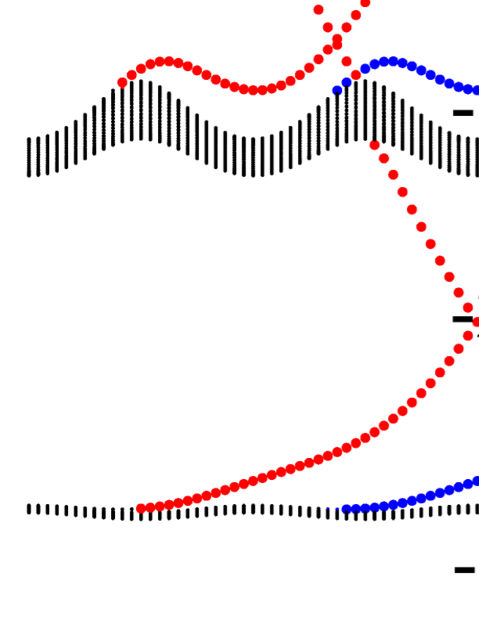
Performing exact numerical diagonalization of the Hamiltonian (24), we obtain the spectrum shown in Fig. 2. In the TI regime, the system hosts a pair of helical edge magnon states. We have checked numerically, that choosing different parameter values changes the spectrum quantitatively but the helical edge states remain, showing that they are indeed topologically stable.

To avoid a breakdown of the sample due to the huge voltage drop resulting from an applied strong electric field, we also consider electric fields and vector potentials ${\mathbf{A}}_{\rm{m}}$ that are periodic in $x$ direction and of saw-tooth shape Nakata et al. (2017b). Using such a periodically extended fields only over a distance that can be much smaller than the sample dimensions or even the electric length $l_{\rm{{\mathcal{E}}}}$, we Nakata et al. (2017b) have seen that the requirement of strong field gradients ${\mathcal{E}}$ needed for creating a quantum Hall effect of magnons in FMs (e.g., Landau levels and the resultant level spacing) can be substantially softened, while still producing well-defined chiral edge magnon states Nakata et al. (2017b), since the magnitude of ${\mathcal{E}}$ for each period remains the same. Periodic fields may be realized by periodically arranging STM tips Freitag et al. (2016); Chen and Wang (2011); Nakata et al. (2017b).

Such periodic potentials are easily implemented in our approach by assuming in Eq. (24) $\theta_{n}=\theta_{1}q\{n/q\}$, with period $q$ (integer) and where $\{\cdot\}$ denotes the fractional part smaller than one. This implies that the periodic vector potential has the form ${\mathbf{A}}_{{\rm{m}}q}=({\mathcal{E}}R_{q}/c)(0,\{x/R_{q}\},0)$, where $R_{q}=qa_{x}$ is the period.

From Fig. 2 we see that for large period $q$ there is a well-developed gap in an almost flat band and with the corresponding edge states, see Fig. 2 (a). If $q$ gets smaller than the electric length, the bulk gap is no longer uniform in momentum, see Figs. 2 (b) and (c). As a result, edge states coexist with bulk modes at different momenta Li et al. (2016); Su et al. (2017), see Fig. 2 (c). However, for fixed values of $k_{y}$, there is still a gap in the spectrum and furthermore, well-defined edge states still exist. Thus, if disorder is weak the edge modes will not couple to the bulk and the Hall conductance will still be dominated by these edge modes, similarly to Weyl semimetals.

Under the assumption that the spin along the $z$ direction remains a good quantum number Z2R ; Klinovaja and Tserkovnyak (2014), we have seen that the key to a nonzero Chern number ${\cal{N}}_{0\sigma}$ is the cyclotron motion of individual magnons. Indeed, the AC phase-induced cyclotron motion leads to edge magnon states (Fig. 2) each giving Halperin (1982); Hatsugai (1993); Shindou et al. (2013a, b); Shindou and Ohe (2014) rise to a non-zero Chern number ${\cal{N}}_{0\sigma}=\sigma$. Therefore, as long as magnons can perform cyclotron motions, the edge magnon state is robust against external perturbation Kane and Mele (2005b); Bernevig and Zhang (2006); Kane and Mele (2005a); Sheng et al. (2005); Murakami (2006); Hasan and Kane (2010); Qi and Zhang (2011) and the relation ${\cal{N}}_{0\uparrow}+{\cal{N}}_{0\downarrow}=0$ between each topological integer Kane and Mele (2005a); Hasan and Kane (2010); Qi and Zhang (2011); Z2R remains valid. Indeed, it has been confirmed experimentally that magnons satisfy Snell’s law at interfaces Tanabe et al. (2014); Stigloher et al. (2016), indicating specular (i.e., elastic) reflection at the boundary to vacuum, and thereby we can expect that magnons form skipping orbits along the boundary like electrons Halperin (1982), giving rise to edge states.

We note that there are still general differences Nakata et al. (2017b) to electrons due to the bosonic nature of the magnons. Due to the Bose-distribution function, even in the presence of topological edge states, the Hall transport coefficients of bulk magnons generally cannot be described in terms of a Chern integer. Only in almost flat bands Nakata et al. (2017b), the Hall coefficients become characterized by such a topological invariant that edge magnon states bring about, while the Hall coefficients are still characterized by the Bose-distribution function (see Sec. III.4). This is in contrast to electronic systems.

III.4 Hall conductances of magnons

In this section, we discuss Hall transport properties of bulk Halperin (1982); Hatsugai (1993); Shindou et al. (2013a, b); Shindou and Ohe (2014) magnons in the AC effect-induced magnonic TIs characterized by a spin-dependent Chern number ${\cal{N}}_{0\sigma}=\sigma$ [Eq. (22)], by making use of the aforementioned mapping between the system and two independent copies Kane and Mele (2005a); Hasan and Kane (2010); Qi and Zhang (2011) of a ferromagnetic ‘quantum’ Hall system Nakata et al. (2017b). We consider the cases where again the total spin along the $z$ direction is a good quantum number. The crystal lattice creates a periodic potential for magnons Ashcroft and Mermin (1976); Kohmoto (1985); Xiao et al. (2010a) $U({\mathbf{r}})=U({\mathbf{r}}+{\mathbf{R}})$ with Bravais lattice vector ${\mathbf{R}}=(a_{x},a_{y})$, which gives rise to a band structure for magnons. In the absence of a magnetic field, $B=0$, the Hamiltonian for spin-$\sigma$ magnons is given by ${\cal{H}}_{\sigma}({\mathbf{r}})={\cal{H}}_{{\rm{m}}\sigma}({\mathbf{r}})+U({\mathbf{r}})$. We then introduce the Bloch Hamiltonian with Bloch wavevector ${\mathbf{k}}=(k_{x},k_{y})$ following Refs. [Kohmoto, 1985; Xiao et al., 2010a; Nakata et al., 2017b], ${\cal{H}}_{{\mathbf{k}}\sigma}\equiv{\rm{e}}^{-i{\mathbf{k}}\cdot{\mathbf{r}}}{\cal{H}}_{\sigma}{\rm{e}}^{i{\mathbf{k}}\cdot{\mathbf{r}}}=[-i\hbar{\mathbf{\nabla}}+\hbar{\mathbf{k}}+\sigma g\mu_{\rm{B}}{\mathbf{A}}_{\rm{m}}({\mathbf{r}})/c]^{2}/2m+\Delta+U({\mathbf{r}})$, where ${\mathbf{A}}_{\rm{m}}$ is the periodically extended vector potential Nakata et al. (2017b). The eigenfunction of the Schrödinger equation ${\cal{H}}_{{\mathbf{k}}\sigma}u_{n{\mathbf{k}}\sigma}({\mathbf{r}})=E_{n{\mathbf{k}}\sigma}u_{n{\mathbf{k}}\sigma}({\mathbf{r}})$ is given by van Hoogdalem et al. (2013); Kohmoto (1985); Xiao et al. (2010a) the magnonic Bloch wave function $u_{n{\mathbf{k}}\sigma}({\mathbf{r}})\equiv{\rm{e}}^{-i{\mathbf{k}}\cdot{\mathbf{r}}}\psi_{n{\mathbf{k}}\sigma}$, where ${\cal{H}}_{\sigma}\psi_{n{\mathbf{k}}\sigma}=E_{n{\mathbf{k}}\sigma}\psi_{n{\mathbf{k}}\sigma}$.

At sufficiently low temperature $k_{{\rm{B}}}T\ll\hbar\omega_{c}$, the lowest mode $n=0$ dominates the dynamics (Fig. 2). In Ref. [Nakata et al., 2017b], where we have studied the magnon bands of a FM in the ‘quantum’ Hall phases realized by the electric field gradient-induced AC effects, we have shown that the lowest magnon band is almost flat on the energy scale set by the temperature van Hoogdalem et al. (2013); Xu et al. (2016); Chisnell et al. (2015), i.e., the band width is much smaller than $k_{{\rm{B}}}T$, and named it almost flat band. Due to this flatness, the lowest band [e.g., Fig. 2 (a)] can be well characterized by its typical energy $E_{0\sigma}^{\ast}$ in the sense that the value of the Bose-distribution function $n_{\rm{B}}(E_{0{\mathbf{k}}\sigma})=({\rm{e}}^{\beta E_{0{\mathbf{k}}}\sigma}-1)^{-1}$ with $\beta\equiv(k_{\rm{B}}T)^{-1}$ can be considered as approximately uniform in the Brillouin zone, $n_{\rm{B}}(E_{0{\mathbf{k}}\sigma})\simeq n_{\rm{B}}(E_{0\sigma}^{*})$, which we will adopt in the subsequent discussion.

Within the linear response regime, the spin and heat Hall current densities for each mode, $j_{y\sigma}$ and $j_{y\sigma}^{Q}$, subjected to a magnetic field gradient Haldane and Arovas (1995); Kovalev et al. (2017) and a temperature one are described by the Onsager matrix

$$\begin{pmatrix}\langle j_{y\sigma}\rangle\\ \langle j_{y\sigma}^{Q}\rangle\end{pmatrix}=\begin{pmatrix}L_{11\sigma}^{yx}&L_{12\sigma}^{yx}\\ L_{21\sigma}^{yx}&L_{22\sigma}^{yx}\end{pmatrix}\begin{pmatrix}\partial_{x}B\\ -\partial_{x}T/T\end{pmatrix}.$$ (25)

Since the band is almost flat, the Hall transport coefficients Matsumoto and Murakami (2011a, b); Nakata et al. (2017b) $L_{ij\sigma}^{yx}$ can be characterized by the Chern number ${\cal{N}}_{0\sigma}=\sigma$,

$$L_{ij\sigma}^{yx}=(k_{\rm{B}}T)^{\eta}(\sigma g\mu_{\rm{B}})^{2-{\eta}}{\cal{C}}_{\eta}\big{(}n_{\rm{B}}(E_{0\sigma}^{\ast})\big{)}\cdot{\cal{N}}_{0\sigma}/h,$$ (26)

where $\eta=i+j-2$, ${\cal{C}}_{0}\big{(}n_{\rm{B}}(E_{0\sigma}^{\ast})\big{)}=n_{\rm{B}}(E_{0\sigma}^{\ast})$, ${\cal{C}}_{1}\big{(}n_{\rm{B}}(E_{0\sigma}^{\ast})\big{)}=[1+n_{\rm{B}}(E_{0\sigma}^{\ast})]{\rm{log}}[1+n_{\rm{B}}(E_{0\sigma}^{\ast})]-n_{\rm{B}}(E_{0\sigma}^{\ast}){\rm{log}}[n_{\rm{B}}(E_{0\sigma}^{\ast})]$, and ${\cal{C}}_{2}\big{(}n_{\rm{B}}(E_{0\sigma}^{\ast})\big{)}=[1+n_{\rm{B}}(E_{0\sigma}^{\ast})]\big{(}{\rm{log}}[1+1/n_{\rm{B}}(E_{0\sigma}^{\ast})]\big{)}^{2}-\big{(}{\rm{log}}[n_{\rm{B}}(E_{0\sigma}^{\ast})]\big{)}^{2}-2{\rm{Li}}_{2}\big{(}-n_{\rm{B}}(E_{0\sigma}^{\ast})\big{)}$. The Onsager reciprocity is satisfied by having $L_{12\sigma}^{yx}=L_{21\sigma}^{yx}$. The coefficient $L_{11\sigma}^{yx}$ is identified with the magnonic spin Hall conductance $G_{\sigma}^{yx}$ arising from each magnon and the total one of the AF is given by $G_{\rm{AF}}^{yx}=\sum_{\sigma}G_{\sigma}^{yx}$. The contribution of each magnon $K_{\sigma}^{yx}$ to the thermal Hall conductance of the AF $K_{\rm{AF}}^{yx}=\sum_{\sigma}K_{\sigma}^{yx}$ is expressed in terms of Onsager coefficients by Nakata et al. (2017b)

$$K_{\sigma}^{yx}=\Big{(}L_{22\sigma}^{yx}-\frac{L_{21\sigma}^{yx}L_{12\sigma}^{yx}}{L_{11\sigma}^{yx}}\Big{)}/T,$$ (27)

where as we have seen in Sec. II, the off-diagonal elements Grunwald and Hajdu (1985); Karavolas and Triberis (1999) similarly arise from the magnon counter-current by the thermally-induced magnetization gradient Johnson and Silsbee (1987); Basso et al. (2016a, b, c); Cornelissen et al. (2016a); Du et al. (2017) $\partial_{x}B_{\sigma}^{\ast}=({L_{12\sigma}^{yx}}/{L_{11\sigma}^{yx}})({\partial_{x}T}/{T})$. See Ref. [Nakata et al., 2017b] for details of the thermal Hall conductance in the ‘quantum’ Hall regime and the Hall coefficient $L_{ij\uparrow}^{yx}$.

In the almost flat band $E_{0\uparrow}^{\ast}\approx E_{0\downarrow}^{\ast}\equiv E_{0}^{\ast}$, the Hall transport coefficient Eq. (26) becomes

$$L_{ij\sigma}^{yx}=\sigma^{2-{\eta}}{L^{\prime}}_{ij}{\cal{N}}_{0\sigma},$$ (28)

where we introduced ${L^{\prime}}_{ij}=(k_{\rm{B}}T)^{\eta}(g\mu_{\rm{B}})^{2-{\eta}}{\cal{C}}_{\eta}\big{(}n_{\rm{B}}(E_{0}^{\ast})\big{)}/h$, which does not depend on the index $\sigma$ with dropping the index $yx$ for convenience. This gives $G_{\sigma}^{yx}=L^{\prime}_{11}{\cal{N}}_{0\sigma}$ and $K_{\sigma}^{yx}=(1/T)(L_{22}^{\prime}-{L_{21}^{\prime}L_{12}^{\prime}}/{L_{11}^{\prime}}){\cal{N}}_{0\sigma}$. Consequently,

$$G_{\rm{AF}}^{yx} = {L^{\prime}}_{11}({\cal{N}}_{0\uparrow}+{\cal{N}}_{0\downarrow}),$$ (29a)

$$K_{\rm{AF}}^{yx} = (1/T)\Big{(}L_{22}^{\prime}-\frac{L_{21}^{\prime}L_{12}^{\prime}}{L_{11}^{\prime}}\Big{)}({\cal{N}}_{0\uparrow}+{\cal{N}}_{0\downarrow}).$$ (29b)

The vanishing of the total Chern number Kane and Mele (2005a); Hasan and Kane (2010); Qi and Zhang (2011) [Eq. (21)], ${\cal{N}}_{0\uparrow}+{\cal{N}}_{0\downarrow}=0$, results in

$$G_{\rm{AF}}^{yx}=0,\ \ \ \ \ K_{\rm{AF}}^{yx}=0.$$ (30)

Thus in contrast to the magnonic Hall system of FMs Nakata et al. (2017b), the thermomagnetic ratio of the AF $K_{\rm{AF}}^{yx}/G_{\rm{AF}}^{yx}$ becomes ill-defined in the sense that the total magnonic spin Hall conductance is zero $G_{\rm{AF}}^{yx}=0$; the WF law Nakata et al. (2015, 2017a) characterized by the liner-in-$T$ behavior becomes violated since the total magnonic thermal Hall conductance vanishes, i.e. $K_{\rm{AF}}^{yx}=0$.

Defining the total magnonic spin and heat Hall current densities, ${\cal{J}}_{y}\equiv\sum_{\sigma}j_{y\sigma}$ and ${\cal{J}}_{y}^{Q}\equiv\sum_{\sigma}j_{y\sigma}^{Q}$, respectively, Eq. (25) is rewritten as

$$\begin{pmatrix}\langle{\cal{J}}_{y}\rangle\\ \langle{\cal{J}}_{y}^{Q}\rangle\end{pmatrix}=\begin{pmatrix}L^{\prime}_{11}({\cal{N}}_{0\uparrow}+{\cal{N}}_{0\downarrow})&L^{\prime}_{12}({\cal{N}}_{0\uparrow}-{\cal{N}}_{0\downarrow})\\ L^{\prime}_{21}({\cal{N}}_{0\uparrow}-{\cal{N}}_{0\downarrow})&L^{\prime}_{22}({\cal{N}}_{0\uparrow}+{\cal{N}}_{0\downarrow})\end{pmatrix}\begin{pmatrix}\partial_{x}B\\ -\frac{\partial_{x}T}{T}\end{pmatrix}.$$

(31)

The component of $L^{\prime}_{12}$ represents the magnonic spin Nernst effect in AFs Cheng et al. (2016); Zyuzin and Kovalev (2016); Shiomi et al. where thermal gradients generate helical magnon Hall transport, and consequently, the total magnonic spin Hall current becomes nonzero. This arises from the opposite magnetic dipole moment $\sigma=\pm 1$ inherent to the N$\acute{{\rm{e}}}$el magnetic order in AF, and the effect is characterized or ensured by the ${\mathbb{Z}}_{2}$ topological invariant Kane and Mele (2005a); Sheng et al. (2005); Hasan and Kane (2010); Qi and Zhang (2011); Z2R [Eq. (22)] ${\cal{Z}}_{0}\equiv({\cal{N}}_{0\uparrow}-{\cal{N}}_{0\downarrow})/2=1$.

The same holds for the reciprocal phenomenon, the magnonic Nernst-Ettinghausen effects Murakami and Okamoto (2017) parametrized by $L^{\prime}_{21}$, while Kane and Mele (2005b); Bernevig and Zhang (2006); Kane and Mele (2005a); Sheng et al. (2005); Murakami (2006); Hasan and Kane (2010); Qi and Zhang (2011). Note that here we refer to the phenomenon described by $L^{\prime}_{11}$ term as ‘magnonic spin Hall effect’ in the bulk AF since it characterizes the magnonic spin Hall conductance $G_{\rm{AF}}^{yx}$ where all magnons subjected to a magnetic field gradient propagate in the same direction and, consequently, the total magnonic spin Hall current becomes zero. This can be qualitatively understood as follows; the particle Hall current density for each magnon $j_{y\sigma}^{\rm{P}}$ is given by $j_{y\sigma}^{\rm{P}}=j_{y\sigma}/(\sigma g\mu_{\rm{B}})$, and Eqs. (25) and (28) provide (see also Table 1)

$$\langle j_{y\sigma}^{\rm{P}}\rangle=\sigma{\cal{N}}_{0\sigma}\frac{{L^{\prime}}_{11}}{g\mu_{\rm{B}}}\partial_{x}B-{\cal{N}}_{0\sigma}\frac{{L^{\prime}}_{12}}{g\mu_{\rm{B}}}\frac{\partial_{x}T}{T}.$$ (32)

Since ${\cal{N}}_{0\sigma}=\sigma$, i.e., ${\cal{N}}_{0\uparrow}=-{\cal{N}}_{0\downarrow}=1$, it shows that thermal gradient generates helical magnon Hall transport in the topological bulk AF where up and down magnons flow in opposite $y$ direction, while all magnons subjected to the magnetic field gradient flow in the same $y$ direction because of the relation $\sigma{\cal{N}}_{0\sigma}=1$. This is in contrast to the topologically trivial bulk AF (Sec. II) where the magnetic field gradient working as a driving force $F_{\sigma}\propto\sigma g\mu_{\rm{B}}$ produces helical magnon currents. The difference arises from each topological integer Kane and Mele (2005b); Bernevig and Zhang (2006); Kane and Mele (2005a); Sheng et al. (2005); Murakami (2006); Hasan and Kane (2010); Qi and Zhang (2011), i.e., the Chern number ${\cal{N}}_{0\sigma}=\sigma$ which leads to $\sigma{\cal{N}}_{0\sigma}=1$. Note that each magnon by itself carries spin $G_{\sigma}^{yx}\not=0$ and heat $K_{\sigma}^{yx}\not=0$, and each mode respectively satisfies the same WF law Nakata et al. (2017b) $K_{\sigma}^{yx}/G_{\sigma}^{yx}=[k_{\rm{B}}/(g\mu_{\rm{B}})]^{2}T$ as the ‘quantum’ Hall system of ferromagnetic magnons. However, due to the relation ${\cal{N}}_{0\uparrow}+{\cal{N}}_{0\downarrow}=0$ between each topological integer Kane and Mele (2005b); Bernevig and Zhang (2006); Kane and Mele (2005a); Sheng et al. (2005); Murakami (2006); Hasan and Kane (2010); Qi and Zhang (2011), magnonic spin and thermal Hall effects in the bulk represented by Eqs. (29a) and (29b), respectively, are prohibited in the topological bulk AF, while the magnonic Nernst-Ettinghausen effects Murakami and Okamoto (2017) shown by the off-diagonals in Eq. (31), $L^{\prime}_{12}$ and $L^{\prime}_{21}$ terms, are characterized or ensured by the ${\mathbb{Z}}_{2}$ topological number ${\cal{Z}}_{0}$ defined in Eq. (22). Thermomagnetic properties of such magnon transport in the topological bulk Mook AF are summarized in Table 1.

Lastly, regarding the linear response to magnetic field gradient, e.g., the total magnonic spin Hall conductance $G_{\rm{AF}}^{yx}$ or $L^{\prime}_{11}$ term, we remark that in Eqs. (29a) and (31), we may still work under the assumption that the relation ${\cal{N}}_{0\uparrow}+{\cal{N}}_{0\downarrow}=0$ between each topological integer Kane and Mele (2005b); Bernevig and Zhang (2006); Kane and Mele (2005a); Sheng et al. (2005); Murakami (2006); Hasan and Kane (2010); Qi and Zhang (2011) is valid since, just for a perturbative driving force, we assume a (negligibly) small magnetic field gradient that does not disturb the cyclotron motion of magnons; thanks to the spin anisotropy-induced energy gap, the energy spectrum is not affected at all and each edge magnon state remains unchanged thereby ensuring the relation ${\cal{N}}_{0\uparrow}+{\cal{N}}_{0\downarrow}=0$ between topological integer, i.e., ${\cal{N}}_{0\sigma}=\sigma$. Recall that in Sec. III.2, we have seen that the cyclotron motion induced by the AC effect leads to the helical edge magnon state characterized by the nonzero Chern number ${\cal{N}}_{0\sigma}=\sigma$. Therefore, as long as each magnon type performs a cyclotron motion, the relation remains unchanged.

IV Estimates for experiments

Observation of spin-wave spin currents Kajiwara et al. (2010); Cornelissen et al. (2015), thermal Hall effect of magnons Onose et al. (2010), magnon planar Hall effect Liu et al. (2017), Snell’s law for spin-wave Tanabe et al. (2014); Stigloher et al. (2016), and electrically-induced AC effect Aharonov and Casher (1984); Mignani (1991); Meier and Loss (2003); Nakata et al. (2014); Ericsson and Sj$\ddot{\rm{o}}$qvist (2001); Nakata et al. (2017b) on a magnonic system Zhang et al. (2014) has been reported. Recently, measurement of magnonic spin conductance Liu et al. (2017) has been reported in Ref. [Cornelissen et al., 2016b] and thermal generation of spin currents in AFs has been established experimentally in Ref. [Seki et al., 2015] using the spin Seebeck effect Uchida et al. (2010); Saitoh et al. (2006); Ohnuma et al. (2013); Adachi et al. (2011, 2010); Xiao et al. (2010b); Dejene et al. (2014); Flipse et al. (2014), with the subsequent report Shiomi et al. ; Cheng et al. (2016); Zyuzin and Kovalev (2016) of magnonic spin Nernst effect in AFs. Moreover, on top of Brillouin light scattering spectroscopy Demokritov et al. (2001, 2006); Agrawal et al. (2013), using infrared camera, the real-time observation of spin-wave propagation is now possible and Ref. [Tanabe et al., 2016] reported the observation of magnon Hall-like effect Liu et al. (2017).

Therefore, we can expect that the observations of the magnonic WF law in the topologically trivial bulk AF and the magnonic QSHE (helical edge magnons) in the topological AF are now within experimental reach Du et al. (2017); Backes et al. (2015); Freitag et al. (2016); Chen and Wang (2011); Mena et al. (2014); An et al. (2013) via measurement schemes proposed in Ref. [Nakata et al., 2017b]. The considered electric field with the constant gradient can be realized by an electric skew-harmonic potential Nakata et al. (2017b) and, while being challenging, it may be realized by STM tips Freitag et al. (2016); Chen and Wang (2011). The resulting magnetization gradient from the applied thermal gradient plays a role of an effective magnetic field gradient and works as a nonequilibrium magnonic spin chemical potential Johnson and Silsbee (1987); Basso et al. (2016a, b, c); Cornelissen et al. (2016a) that has been established experimentally in Ref. [Du et al., 2017].

For an estimate, we assume the following experiment parameter values Artman et al. (1965); Kota and Imamura (2017) for ${\rm{Cr}}_{2}{\rm{O}}_{3}$, $J=15$meV, ${\cal{K}}=0.03$meV, $S=3/2$, $g=2$, ${\mathcal{E}}=1$V/nm², and $a=0.5$nm. This provides the Landau gap $\hbar\omega_{c}=1\mu$eV and $l_{\rm{{\mathcal{E}}}}=0.7\mu$m [Eqs. (17) and (18)], with which the magnonic QSHE and helical edge magnons could be observed at $T\lesssim 10$mK. At these low temperatures, effects of magnon-magnon and magnon-phonon interactions can be expected to become negligible Nakata et al. (2015); Adachi et al. (2010); Prasai et al. (2017). An alternative platform to look for topological magnon Hall effects would be skyrmion-like lattices of AFs Zhang et al. (2016); Barker and Tretiakov (2016); G$\ddot{\rm{o}}$bel et al. (2017) with Dzyaloshinskii-Moriya (DM) Dzyaloshinskii (1958); Moriya (1960a, b) interaction where the N$\acute{{\rm{e}}}$el order parameter varies slowly compared to the typical wavelength of magnons (i.e., spin-waves). In Ref. [van Hoogdalem et al., 2013] (see Appendix D for details), we have seen that the low-energy magnetic excitations in the skyrmion lattice are magnons and the DM interaction Mook et al. (2015); Zhang et al. (2013); Katsura et al. (2005) produces intrinsically a vector potential analogous to ${\mathbf{A}}_{\rm{m}}$ which reduces to the same form as Eq. (12). Assuming experimental parameter values Nagaosa and Tokura (2013); Yu et al. (2010); Han et al. (2010) (see Ref. [Nakata et al., 2017b] for details), Landau gaps on the order of a few meVs could be reached. Since the Hamiltonian for an AF in a skyrmion-like lattice where the N$\acute{{\rm{e}}}$el order varies slowly (compared to the typical wavelength of spin-waves) also reduces to the qualitatively same form as Eq. (12), we expect that the topological magnon Hall effects could be observed at $T\lesssim{\cal{O}}(10)$K in such AFs Zhang et al. (2016); Barker and Tretiakov (2016); G$\ddot{\rm{o}}$bel et al. (2017). The temperature, however, should be low enough to make spin-phonon and magnon-magnon contributions negligible Nakata et al. (2015); Adachi et al. (2010); Prasai et al. (2017). As to the magnonic WF law in the topologically trivial bulk AFs, the energy gap amounts to $\Delta=4$meV and thus the magnonic WF law may be observed at $T=40$K ($k_{\rm{B}}T=\Delta$). However, again, the temperature should be low enough Pho to make spin-phonon and magnon-magnon contributions negligible Nakata et al. (2015); Adachi et al. (2010); Prasai et al. (2017). Therefore we expect that the effect becomes observable at low temperature $T\lesssim{\cal{O}}(1)$K.

Given these estimates, we conclude that the observations of the magnonic and topological phenomena in AFs as proposed in this work, while being challenging, seem within experimental reach Kent .

V Summary

Under the assumption that the spin along the $z$ direction remains a good quantum number, we have studied thermomagnetic properties of helical transport of magnons with the opposite magnetic dipole moment inherent to the N$\acute{{\rm{e}}}$el order both in topologically trivial and nontrivial bulk AFs. Since the quantum-mechanical dynamics of magnons in the insulating AF is described as the combination of independent copies of that in FMs, we found that both topologically trivial magnets satisfy the same magnonic WF law, exhibiting a linear-in-$T$ behavior at sufficiently low temperatures, while the law becomes violated in the topological bulk AF due to the topological invariant that helical edge magnon states bring about. In the electric field gradient-induced AC effect, up and down magnons form the same Landau energy level and perform cyclotron motion with the same frequency but in opposite directions giving rise to helical edge magnon states, i.e., QSHE of edge magnons, and the AF becomes characterized by the ${\mathbb{Z}}_{2}$ topological number consisting of the Chern integer that each edge state brings about and the AF can be identified as a bosonic version of a TI. In the almost flat band inherent to the electrically-induced topological AF, the magnonic spin and thermal Hall effects of bulk magnons are prohibited by the topological integer, while the Nernst-Ettinghausen effects are ensured by the ${\mathbb{Z}}_{2}$ topological invariant. The relation between each topological integer is robust against external perturbation as long as magnons can perform cyclotron motion giving the helical edge magnon states.

Finally, it would be interesting to test our predictions experimentally.

VI Discussion

To conclude a few comments on our approach are in order. Instead of deriving the helical edge states directly from the spin Hamiltonian in the presence of electric fields as done previously for FMs Nakata et al. (2017b), here we first derive the magnon approximation of the spin Hamiltonian in the continuum limit and then introduce the AC phase. The resulting Hamiltonian with quadratic magnon dispersion is then analyzed numerically by introducing the corresponding TBR. Throughout this paper we have thus restricted our consideration to AFs where within the long wave-length approximation the dispersion becomes gapped and parabolic, and the dynamics of magnons in the AF can be described as the combination of two independent copies of the dynamics of magnons in a FM for each mode $\sigma=\pm 1$. The helical edge states we found in this approximation are topologically stable and thus their emergence does not depend on the microscopic details as long as the gap remains open. Still, a general treatment of AFs (beyond the parabolic dispersion regime, on different lattices, e.g., on a triangular spin lattice in the presence of frustration etc.) remains an open issue and deserves further study.

Lastly we remark that due to the opposite magnetic dipole moments of up and down magnons associated with the magnetic N$\acute{{\rm{e}}}$el order in AFs, the $\sigma$-dependence is simply added to the TBR Eq. (23). This $\sigma$-dependence, while being a small theoretical difference from the FMs Nakata et al. (2017b), produces qualitatively new phenomena in AFs such as helical edge magnon states and the violation of the magnonic WF law Nakata et al. (2017b). We stress that this simplicity of the $\sigma$-dependence is specific to the time-independent case considered here. In contrast, when the electric field becomes time-dependent (e.g., in the presence of laser pulses) the AC gauge potential becomes also time-dependent and the $\sigma$-dependence could be controlled or even vanish for some ac electric fields. This opens up a new control on the topological phase. It will thus be interesting to study time-dependent effects in these systems in more detail.

Appendix A Magnons in AFs

In this Appendix, we provide some details of the straightforward treatment of AFs Altland and Simons (2006); Kubo (1952); Anderson (1952) showing that their N$\acute{{\rm{e}}}$el order provides up and down magnons, i.e., ‘magnetically charged’ bosonic quasiparticles carrying opposite magnetic dipole moments $\sigma g\mu_{\rm{B}}{\bf e}_{z}$. An external magnetic field ${\mathbf{B}}=B{\mathbf{e}}_{z}$ couples with spins via the Zeeman interaction given by ${\cal{H}}_{B}=-g\mu_{\rm{B}}B\sum_{l}S_{l}^{z}$. Assuming spins in the AF form the N$\acute{{\rm{e}}}$el order along $z$ direction, and using the sublattice-dependent Holstein-Primakoff Holstein and Primakoff (1940); Altland and Simons (2006); Cheng et al. (2016); Zyuzin and Kovalev (2016) transformation, $S_{i{\rm{A}}}^{z}=S-a_{i}^{\dagger}a_{i}$, $S_{j{\rm{B}}}^{z}=-S+b_{j}^{\dagger}b_{j}$, with $[a_{i},a_{j}^{\dagger}]=\delta_{i,j}$ and $[b_{i},b_{j}^{\dagger}]=\delta_{i,j}$, we find for the $z$ component of the total spin Cheng et al. (2016) $S^{z}\equiv\sum_{l}S_{l}^{z}=\sum_{i}(S_{i{\rm{A}}}^{z}+S_{i{\rm{B}}}^{z})=\sum_{i}(-a_{i}^{\dagger}a_{i}+b_{i}^{\dagger}b_{i})$. After Fourier transformation $S^{z}=\sum_{\mathbf{k}}(-a_{\mathbf{k}}^{\dagger}a_{\mathbf{k}}+b_{\mathbf{k}}^{\dagger}b_{\mathbf{k}})$, the Hamiltonian becomes ${\cal{H}}_{B}=g\mu_{\rm{B}}B\sum_{\mathbf{k}}(a_{\mathbf{k}}^{\dagger}a_{\mathbf{k}}-b_{\mathbf{k}}^{\dagger}b_{\mathbf{k}})$. Using a Bogoliubov transformation

$$\begin{pmatrix}a_{\mathbf{k}}^{\dagger}\\ b_{\mathbf{k}}\end{pmatrix}=\cal{M}\begin{pmatrix}{\cal{A}}_{\mathbf{k}}^{\dagger}\\ {\cal{B}}_{\mathbf{k}}\end{pmatrix},\begin{pmatrix}a_{\mathbf{k}}\\ b_{\mathbf{k}}^{\dagger}\end{pmatrix}=\cal{M}\begin{pmatrix}{\cal{A}}_{\mathbf{k}}\\ {\cal{B}}_{\mathbf{k}}^{\dagger}\end{pmatrix}$$ (33)

with the coefficient matrix $\cal{M}$ defined by

$$\cal{M}=\begin{pmatrix}{\rm{cosh}}\vartheta_{\mathbf{k}}&-{\rm{sinh}}\vartheta_{\mathbf{k}}\\ -{\rm{sinh}}\vartheta_{\mathbf{k}}&{\rm{cosh}}\vartheta_{\mathbf{k}}\end{pmatrix},$$ (34)

the Hamiltonian $\cal{H}$ in the main text becomes diagonal Altland and Simons (2006); Kubo (1952); Anderson (1952), ${\cal{H}}=\sum_{\mathbf{k}}\hbar\omega_{\mathbf{k}}({\cal{A}}_{\mathbf{k}}^{\dagger}{\cal{A}}_{\mathbf{k}}+{\cal{B}}_{\mathbf{k}}^{\dagger}{\cal{B}}_{\mathbf{k}})$, in terms of Bogoliubov quasiparticle operators, ${\cal{A}}_{\mathbf{k}}$ and ${\cal{B}}_{\mathbf{k}}$, satisfying bosonic commutation relations $[{\cal{A}}_{\mathbf{k}},{\cal{A}}_{{\mathbf{k^{\prime}}}}^{\dagger}]=\delta_{{\mathbf{k}},{\mathbf{k^{\prime}}}}$ and $[{\cal{B}}_{\mathbf{k}},{\cal{B}}_{{\mathbf{k^{\prime}}}}^{\dagger}]=\delta_{{\mathbf{k}},{\mathbf{k^{\prime}}}}$, where ${\rm{tanh}}(2\vartheta_{\mathbf{k}})=\gamma_{\mathbf{k}}/(1+\kappa)$, $\gamma_{\mathbf{k}}=(1/\rho)\sum_{m=1}^{\rho}{\rm{e}}^{-i{\mathbf{k}}\cdot{\bm{\delta}}_{m}}$, the coordination number $\rho=2d$, and ${\bm{\delta}}_{m}$ the relative coordinate vector that connects the nearest neighboring sites. The $z$ component of the total spin is rewritten as $S^{z}=\sum_{\mathbf{k}}(-a_{\mathbf{k}}^{\dagger}a_{\mathbf{k}}+b_{\mathbf{k}}^{\dagger}b_{\mathbf{k}})=\sum_{\mathbf{k}}(-{\cal{A}}_{\mathbf{k}}^{\dagger}{\cal{A}}_{\mathbf{k}}+{\cal{B}}_{\mathbf{k}}^{\dagger}{\cal{B}}_{\mathbf{k}})$ and thereby ${\cal{H}}_{B}=g\mu_{\rm{B}}B\sum_{\mathbf{k}}(a_{\mathbf{k}}^{\dagger}a_{\mathbf{k}}-b_{\mathbf{k}}^{\dagger}b_{\mathbf{k}})=g\mu_{\rm{B}}B\sum_{\mathbf{k}}({\cal{A}}_{\mathbf{k}}^{\dagger}{\cal{A}}_{\mathbf{k}}-{\cal{B}}_{\mathbf{k}}^{\dagger}{\cal{B}}_{\mathbf{k}})$. Therefore, it can be seen that the ${\cal{A}}$- (${\cal{B}}$-) magnon carries $\sigma=-1$ ($+1$) spin angular momentum along the $z$ direction and can be identified with down and up magnons, respectively.

In the absence of the magnetic field, $B=0$, these up and down magnons are degenerate and the energy dispersion Kubo (1952); Anderson (1952) is given by $\hbar\omega_{{\mathbf{k}}}=2JdS\sqrt{(1+\kappa)^{2}-\gamma_{\mathbf{k}}^{2}}$. Within the long wave-length approximation, it becomes $\gamma_{\mathbf{k}}^{2}=1-(ak)^{2}/d$ for $\mid{\mathbf{k}}\mid=k$ and thereby assuming a spin anisotropy Artman et al. (1965); Kota and Imamura (2017) at low temperature, the dispersion becomes parabolic in terms of $k$ and reduces to the form $\hbar\omega_{{\mathbf{k}}}=Dk^{2}+\Delta$ with $D=JSa^{2}/\sqrt{\kappa^{2}+2\kappa}$ which is used in the main text. Note that the dispersion becomes linear in terms of $k$, $\hbar\omega_{{\mathbf{k}}}\propto k$, when there is no spin anisotropy ${\cal{K}}=0$, i.e., $\kappa=0$.

Lastly we remark that the $z$ component of spins is a good quantum number Z2R of our system, which commutes with the original spin Hamiltonian [Eq. (1)]. Therefore regardless of the analytical approach taken, e.g., noninteracting magnon picture Kubo (1952); Anderson (1952) using the Holstein-Primakoff transformation we adopted throughout this work, the excitations should have a well-defined spin $z$ component. The Hamiltonian and the spin $z$ component are simultaneously diagonalizable. Therefore it can be expected that, apart from any magnon picture, two well-defined opposite spin modes and the helical nature of the resultant edge spin modes should survive in any case at sufficiently low temperatures where phonons die out Adachi et al. (2010); Prasai et al. (2017).

Appendix B Boltzmann equation for magnons

In this Appendix, we provide some details of the straightforward calculation for the Onsager coefficients $L_{ij\sigma}$ in the topologically trivial bulk AF. Assuming the system is slightly out of equilibrium and using the Boltzmann transport equation Basso et al. (2016a, b, c) given in Ref. [Mahan, 2000], the Bose-distribution function of magnons $f_{{\mathbf{k}}\sigma}$ becomes $f_{{\mathbf{k}}\sigma}=f^{0}_{{\mathbf{k}}\sigma}+g_{{\mathbf{k}}\sigma}$ where $f^{0}_{{\mathbf{k}}\sigma}=({\rm{e}}^{\beta\epsilon_{{{\mathbf{k}}\sigma}}}-1)^{-1}$ with $\epsilon_{{{\mathbf{k}}\sigma}}=\hbar\omega_{{\mathbf{k}}\sigma}$ is the equilibrium distribution while the deviation from equilibrium $g_{{\mathbf{k}}\sigma}=f_{{\mathbf{k}}\sigma}-f^{0}_{{\mathbf{k}}\sigma}$ is given by $g_{{\mathbf{k}}\sigma}=\tau{\mathbf{v}}_{{\mathbf{k}}}\cdot[-\sigma g\mu_{\rm{B}}{\mathbf{\nabla}}B+(\epsilon_{{{\mathbf{k}}\sigma}}/T){\mathbf{\nabla}}T](\partial f^{0}_{{\mathbf{k}}\sigma}/\partial\epsilon_{{{\mathbf{k}}\sigma}})$ within the liner response regime, where ${\mathbf{v}}_{{\mathbf{k}}}=\partial\epsilon_{{\mathbf{k}}\sigma}/\partial\hbar{\mathbf{k}}$ is the velocity and $\tau$ a phenomenologically introduced relaxation time of magnons, mainly due to nonmagnetic impurity scatterings and thereby we may assume it to be a constant at low temperature. The resulting particle, spin, and heat currents for each magnon mode, ${\mathbf{j}}_{\sigma}^{\rm{P}}$, ${\mathbf{j}}_{\sigma}$, ${\mathbf{j}}_{\sigma}^{Q}$, respectively, are given by ${\mathbf{j}}_{\sigma}^{\rm{P}}=\int[d^{3}{\mathbf{k}}/(2\pi)^{3}]{\mathbf{v}}_{{\mathbf{k}}}g_{{\mathbf{k}}\sigma}$, ${\mathbf{j}}_{\sigma}=\int[d^{3}{\mathbf{k}}/(2\pi)^{3}]\sigma g\mu_{\rm{B}}{\mathbf{v}}_{{\mathbf{k}}}g_{{\mathbf{k}}\sigma}$, ${\mathbf{j}}_{\sigma}^{Q}=\int[d^{3}{\mathbf{k}}/(2\pi)^{3}]\epsilon_{{\mathbf{k}}\sigma}{\mathbf{v}}_{{\mathbf{k}}}g_{{\mathbf{k}}\sigma}$. Assuming spatial isotropy $|k_{x}|=|k_{y}|=|k_{z}|$ for ${\mathbf{k}}=(k_{x},k_{y},k_{z})$ and performing the Gaussian integrals, the Onsager coefficients $L_{ij\sigma}$ shown in the main text are obtained.

Appendix C Cyclotron motion of magnons

In this Appendix, we provide for completeness some details of the straightforward calculation showing that the dynamics of magnons with the opposite magnetic dipole moments $\sigma g\mu_{\rm{B}}{\mathbf{e}}_{z}$ are identical except that the resulting chirality of the magnon propagation becomes opposite [Fig. 1 (b)]. Using the correspondence explained in the main text, the calculation becomes analogous to the one for electrons Mahan (2000); Ezawa (2013), and especially it parallels the one for ferromagnetic magnons given in Ref. [Nakata et al., 2017b] except that we have now two magnon modes with opposite magnetic dipole moment ($\sigma=\pm 1$). Introducing operators analogous to a covariant momentum ${\hat{{\mathbf{\Pi}}}}_{\sigma}\equiv\hat{{\mathbf{p}}}+\sigma g\mu_{\rm{B}}{\mathbf{A}}_{\rm{m}}/c=(\Pi_{x\sigma},\Pi_{y\sigma})$, which satisfy $[\Pi_{x\sigma},\Pi_{y\sigma}]=-i\sigma\hbar^{2}/l_{\rm{{\mathcal{E}}}}^{2}$, and dropping the irrelevant constant, the Hamiltonian for each mode can be rewritten as ${\cal{H}}_{{\rm{m}}\sigma}=(\Pi_{x\sigma}^{2}+\Pi_{y\sigma}^{2})/2m$. Next, introducing the operators $A_{\sigma}\equiv l_{\rm{{\mathcal{E}}}}(\Pi_{x\sigma}-i\sigma\Pi_{y\sigma})/\sqrt{2}\hbar$ and $A_{\sigma}^{\dagger}\equiv l_{\rm{{\mathcal{E}}}}(\Pi_{x\sigma}+i\sigma\Pi_{y\sigma})/\sqrt{2}\hbar$, which satisfy bosonic commutation relations, $[A_{\sigma},A_{\sigma}^{\dagger}]=1$ with the remaining commutators vanishing, the Hamiltonian becomes ${\cal{H}}_{{\rm{m}}\sigma}=\hbar\omega_{c}(A_{\sigma}^{\dagger}A_{\sigma}+1/2)$. Indeed, introducing Ezawa (2013) the guiding-center coordinate by $X_{\sigma}=x-\sigma l_{\rm{{\mathcal{E}}}}^{2}\Pi_{y\sigma}/\hbar$ and $Y_{\sigma}=y+\sigma l_{\rm{{\mathcal{E}}}}^{2}\Pi_{x\sigma}/\hbar$, which satisfy $[X_{\sigma},Y_{\sigma}]=i\sigma l_{\rm{{\mathcal{E}}}}^{2}$ with $dX_{\sigma}/dt=dY_{\sigma}/dt=0$ indicating that the drift velocity vanishes in the absence of the magnetic field gradient, the time-evolution of the relative coordinate ${\mathbf{R}}_{{\rm{{\mathcal{E}}}}\sigma}=({\cal{R}}_{x\sigma},{\cal{R}}_{y\sigma})\equiv(-l_{\rm{{\mathcal{E}}}}^{2}\Pi_{y\sigma}/\hbar,l_{\rm{{\mathcal{E}}}}^{2}\Pi_{x\sigma}/\hbar)$ becomes $d({\cal{R}}_{x\sigma}+i{\cal{R}}_{y\sigma})/dt=i\sigma\omega_{c}({\cal{R}}_{x\sigma}+i{\cal{R}}_{y\sigma})$. Thus in the presence of an electric field gradient, two magnons form the same Landau level and perform cyclotron motion with the same frequency, but propagate in opposite directions due to the opposite magnetic dipole moment $\sigma g\mu_{\rm{B}}{\mathbf{e}}_{z}$ [Fig. 1 (b)].

Appendix D Landau levels in topological magnets

In this Appendix, we provide some insight into the magnons in DM interaction-induced skyrmion-like structures where the DM Dzyaloshinskii (1958); Moriya (1960a, b) interaction provides Katsura et al. (2005) an effective AC phase. In Ref. [van Hoogdalem et al., 2013], we have seen that the low-energy magnetic excitations in the skyrmion lattice are magnons and the DM interaction produces a textured equilibrium magnetization that works intrinsically as a vector potential analogous to ${\mathbf{A}}_{\rm{m}}$. The Hamiltonian of magnons indeed reduces to the same form of Eq. (12) with the analog of the Landau gauge that produces the Landau energy level [Eq. (16)]. Assuming the magnitude of the DM interaction Nagaosa and Tokura (2013); Yu et al. (2010); Han et al. (2010); Tacchi et al. (2017); Mulkers et al. (2017) $\Gamma_{\rm{DM}}$, the Landau energy level spacing is given by van Hoogdalem et al. (2013) $(4JS/\sqrt{3}\pi)(\Gamma_{\rm{DM}}/J)^{2}$; see Refs. [van Hoogdalem et al., 2013; Nakata et al., 2017b] for details. Using the correspondence with the Landau energy level spacing by electric field gradient-induced AC effect $\hbar\omega_{\rm{c}}$ [Eqs. (16) and (17)], it can be seen to be qualitatively identified with an effective inner electric field gradient QSH and the magnitude is estimated by ${\cal{E}}_{\rm{DM}}=[2/(\sqrt{3}\pi a^{2})](\hbar c^{2}/g\mu_{\rm{B}})(\Gamma_{\rm{DM}}/J)^{2}\propto\Gamma_{\rm{DM}}^{2}$. This indicates that the DM interaction produces a slowly-varying textured equilibrium magnetization that provides an effective AC phase and in such a skyrmion-like structure, it works as an effective, fictitious, and intrinsic electric field gradient ${\cal{E}}_{\rm{DM}}={\cal{O}}(10^{2})$V/nm² of very large magnitude van Hoogdalem et al. (2013); Katsura et al. (2005). Note that the key to edge magnon states is the vector potential ${\mathbf{A}}_{\rm{m}}$ that globally satisfies the relation [Eq. (13)] ${\mathbf{\nabla}}\times{\mathbf{A}}_{\rm{m}}=({{\mathcal{E}}}/{c}){\mathbf{e}}_{z}$ where magnons experience the vector potential macroscopically, leading to cyclotron motion.

References

- Demokritov et al. (2006) S. O. Demokritov, V. E. Demidov, O. Dzyapko, G. A. Melkov, A. A. Serga, B. Hillebrands, and A. N. Slavin, Nature 443, 430 (2006).
- Chumak et al. (2015) A. V. Chumak, V. I. Vasyuchka, A. A. Serga, and B. Hillebrands, Nat. Phys. 11, 453 (2015).
- Serga et al. (2010) A. A. Serga, A. V. Chumak, and B. Hillebrands, J. Phys. D 43, 264002 (2010).
- Nakata et al. (2017a) K. Nakata, P. Simon, and D. Loss, J. Phys. D: Appl. Phys. 50, 114004 (2017a).
- Kajiwara et al. (2010) Y. Kajiwara, K. Harii, S. Takahashi, J. Ohe, K. Uchida, M. Mizuguchi, H. Umezawa, H. Kawai, K. Ando, K. Takanashi, et al., Nature 464, 262 (2010).
- Onose et al. (2010) Y. Onose, T. Ideue, H. Katsura, Y. Shiomi, N. Nagaosa, and Y. Tokura, Science 329, 297 (2010).
- Cornelissen et al. (2015) L. J. Cornelissen, J. Liu, R. A. Duine, J. B. Youssef, and B. J. van Wees, Nat. Phys. 11, 1022 (2015).
- Liu et al. (2017) J. Liu, L. J. Cornelissen, J. Shan, T. Kuschel, and B. J. van Wees, Phys. Rev. B 95, 140402(R) (2017).
- Tanabe et al. (2014) K. Tanabe, R. Matsumoto, J. Ohe, S. Murakami, T. Moriyama, D. Chiba, K. Kobayashi, and T. Ono, Appl. Phys. Express 7, 053001 (2014).
- Stigloher et al. (2016) J. Stigloher, M. Decker, H. Krner, K. Tanabe, T. Moriyama, T. Taniguchi, H. Hata, M. Madami, G. Gubbiotti, K. Kobayashi, et al., Phys. Rev. Lett. 117, 037204 (2016).
- Aharonov and Casher (1984) Y. Aharonov and A. Casher, Phys. Rev. Lett. 53, 319 (1984).
- Mignani (1991) R. Mignani, J. Phys. A: Math. Gen. 24, L421 (1991).
- Meier and Loss (2003) F. Meier and D. Loss, Phys. Rev. Lett. 90, 167204 (2003).
- Nakata et al. (2014) K. Nakata, K. A. van Hoogdalem, P. Simon, and D. Loss, Phys. Rev. B 90, 144419 (2014).
- Ericsson and Sjqvist (2001) M. Ericsson and E. Sjqvist, Phys. Rev. A 65, 013607 (2001).
- Liu and Vignale (2011) T. Liu and G. Vignale, Phys. Rev. Lett. 106, 247203 (2011).
- Liu and Vignale (2012) T. Liu and G. Vignale, J. Appl. Phys. 111, 083907 (2012).
- Aharonov and Bohm (1959) Y. Aharonov and D. Bohm, Phys. Rev. 115, 485 (1959).
- Loss et al. (1990) D. Loss, P. Goldbart, and A. V. Balatsky, Phys. Rev. Lett. 65, 1655 (1990).
- Loss and Goldbart (1992) D. Loss and P. M. Goldbart, Phys. Rev. B 45, 13544 (1992).
- Zhang et al. (2014) X. Zhang, T. Liu, M. E. Flatte, and H. X. Tang, Phys. Rev. Lett. 113, 037202 (2014).
- v. Klitzing et al. (1980) K. v. Klitzing, G. Dorda, and M. Pepper, Phys. Rev. Lett. 45, 494 (1980).
- Thouless et al. (1982) D. J. Thouless, M. Kohmoto, M. P. Nightingale, and M. den Nijs, Phys. Rev. Lett. 49, 405 (1982).
- Kohmoto (1985) M. Kohmoto, Ann. Phys. 160, 343 (1985).
- Pankratov (1987) O. A. Pankratov, Phys. Lett. A 121, 360 (1987).
- Haldane (1988) F. D. M. Haldane, Phys. Rev. Lett. 61, 2015 (1988).
- Volovik and Yakovenko (1989) G. E. Volovik and V. M. Yakovenko, J. Phys.: Condens. Matter 1, 5263 (1989).
- Klinovaja et al. (2015) J. Klinovaja, Y. Tserkovnyak, and D. Loss, Phys. Rev. B 91, 085426 (2015).
- Halperin (1982) B. I. Halperin, Phys. Rev. B 25, 2185 (1982).
- Hatsugai (1993) Y. Hatsugai, Phys. Rev. Lett. 71, 3697 (1993).
- Kane and Mele (2005a) C. Kane and E. Mele, Phys. Rev. Lett. 95, 146802 (2005a).
- Kane and Mele (2005b) C. Kane and E. Mele, Phys. Rev. Lett. 95, 226801 (2005b).
- Bernevig and Zhang (2006) B. A. Bernevig and S. C. Zhang, Phys. Rev. Lett. 96, 106802 (2006).
- Hasan and Kane (2010) M. Z. Hasan and C. L. Kane, Rev. Mod. Phys. 82, 3045 (2010).
- Qi and Zhang (2011) X. L. Qi and S. C. Zhang, Rev. Mod. Phys. 83, 1057 (2011).
- (36) B. Zeng, X. Chen, D. L. Zhou, and X. G. Wen, arXiv:1508.02595.
- Senthil (2015) T. Senthil, Annu. Rev. Condens. Matter Phys. 6, 299 (2015).
- Senthil and Levin (2013) T. Senthil and M. Levin, Phys. Rev. Lett. 110, 046801 (2013).
- Sheng et al. (2005) D. N. Sheng, Z. Y. Weng, L. Sheng, and F. D. M. Haldane, Phys. Rev. Lett. 97, 036808 (2005).
- Murakami (2006) S. Murakami, Phys. Rev. Lett. 97, 236805 (2006).
- T. Wolfram and R. E. De Wames (1952) T. Wolfram and R. E. De Wames, Phys. Rev. 185, 762 (1952).
- Anderson (1952) P. W. Anderson, Phys. Rev. 86, 694 (1952).
- Kubo (1952) R. Kubo, Phys. Rev. 87, 568 (1952).
- Jungwirth et al. (2016) T. Jungwirth, X. Marti, P. Wadley, and J. Wunderlich, Nat. Nanotech. 11, 231 (2016).
- Gomonaya and Loktev (2014) E. V. Gomonaya and V. M. Loktev, Low Temp. Phys. 40, 17 (2014).
- Nakata et al. (2017b) K. Nakata, J. Klinovaja, and D. Loss, Phys. Rev. B 95, 125429 (2017b).
- Nakata et al. (2015) K. Nakata, P. Simon, and D. Loss, Phys. Rev. B 92, 134425 (2015).
- van Hoogdalem et al. (2013) K. A. van Hoogdalem, Y. Tserkovnyak, and D. Loss, Phys. Rev. B 87, 024402 (2013).
- Xiao et al. (2010a) D. Xiao, M.-C. Chang, and Q. Niu, Rev. Mod. Phys. 82, 1959 (2010a).
- Franz and Wiedemann (1853) R. Franz and G. Wiedemann, Annalen der Physik 165, 497 (1853).
- Seki et al. (2015) S. Seki, T. Ideue, M. Kubota, Y. Kozuka, R. Takagi, M. Nakamura, Y. Kaneko, M. Kawasaki, and Y. Tokura, Phys. Rev. Lett. 115, 266601 (2015).
- Uchida et al. (2010) K. Uchida, J. Xiao, H. Adachi, J. Ohe, S. Takahashi, J. Ieda, T. Ota, Y. Kajiwara, H. Umezawa, H. Kawai, et al., Nat. Mater. 9, 894 (2010).
- Saitoh et al. (2006) E. Saitoh, M. Ueda, H. Miyajima, and G. Tatara, Appl. Phys. Lett. 88, 182509 (2006).
- Ohnuma et al. (2013) Y. Ohnuma, H. Adachi, E. Saitoh, and S. Maekawa, Phys. Rev. B 87, 014423 (2013).
- Adachi et al. (2011) H. Adachi, J. Ohe, S. Takahashi, and S. Maekawa, Phys. Rev. B 83, 094410 (2011).
- Adachi et al. (2010) H. Adachi, K. Uchida, E. Saitoh, J. Ohe, S. Takahashi, and S. Maekawa, Apply. Phys. Lett. 97, 252506 (2010).
- Xiao et al. (2010b) J. Xiao, G. E. W. Bauer, K. Uchida, E. Saitoh, and S. Maekawa, Phys. Rev. B 81, 214418 (2010b).
- Dejene et al. (2014) F. K. Dejene, J. Flipse, and B. J. van Wees, Phys. Rev. B 90, 180402(R) (2014).
- Flipse et al. (2014) J. Flipse, F. K. Dejene, D. Wagenaar, G. E. Bauer, J. B. Youssef, and B. J. van Wees, Phys. Rev. Lett. 113, 027601 (2014).
- Cheng et al. (2016) R. Cheng, S. Okamoto, and D. Xiao, Phys. Rev. Lett. 117, 217202 (2016).
- Zyuzin and Kovalev (2016) V. A. Zyuzin and A. A. Kovalev, Phys. Rev. Lett. 117, 217203 (2016).
- (62) Y. Shiomi, R. Takashima, and E. Saitoh, arXiv:1706.03978.
- van Hoogdalem and Loss (2011) K. A. van Hoogdalem and D. Loss, Phys. Rev. B 84, 024402 (2011).
- Normand et al. (2000) B. Normand, J. Kyriakidis, and D. Loss, Ann. Phys. (Leipzig) 9, 133 (2000).
- Prasai et al. (2017) N. Prasai, B. A. Trump, G. G. Marcus, A. Akopyan, S. X. Huang, T. M. McQueen, and J. L. Cohn, Phys. Rev. B 95, 224407 (2017).
- Altland and Simons (2006) A. Altland and B. Simons, Condensed Matter Field Theory (Cambridge University Press, 2006).
- Artman et al. (1965) J. O. Artman, J. C. Murphy, and S. Foner, Phys. Rev. 138, A912 (1965).
- Kota and Imamura (2017) Y. Kota and H. Imamura, Appl. Phys. Express 10, 013002 (2017).
- Holstein and Primakoff (1940) T. Holstein and H. Primakoff, Phys. Rev. 58, 1098 (1940).
- Mahan (2000) G. D. Mahan, Many-Particle Physics (Kluwer Academic, Plenum Publishers, Third edition, 2000).
- Basso et al. (2016a) V. Basso, E. Ferraro, A. Magni, A. Sola, M. Kuepferling, and M. Pasquale, Phys. Rev. B 93, 184421 (2016a).
- Basso et al. (2016b) V. Basso, E. Ferraro, and M. Piazzi, Phys. Rev. B 94, 144422 (2016b).
- Basso et al. (2016c) V. Basso, E. Ferraro, and M. Piazzi, Phys. Rev. B 94, 179907 (2016c).
- Ashcroft and Mermin (1976) N. W. Ashcroft and N. D. Mermin, Solid State Physics (Brooks Cole, 1976).
- Bauer et al. (2012) G. E. W. Bauer, E. Saitoh, and B. J. van Wees, Nat.Mater 11, 391 (2012).
- Grunwald and Hajdu (1985) A. Grunwald and J. Hajdu, Z. Phys. B 60, 235 (1985).
- Karavolas and Triberis (1999) V. C. Karavolas and G. P. Triberis, Phys. Rev. B 59, 7590 (1999).
- Johnson and Silsbee (1987) M. Johnson and R. H. Silsbee, Phys. Rev. B 35, 4959 (1987).
- Cornelissen et al. (2016a) L. J. Cornelissen, K. J. H. Peters, G. E. W. Bauer, R. A. Duine, and B. J. van Wees, Phys. Rev. B 94, 014412 (2016a).
- Du et al. (2017) C. Du, T. V. der Sar, T. X. Zhou, P. Upadhyaya, F. Casola, H. Zhang, M. C. Onbasli, C. A. Ross, R. L. Walsworth, Y. Tserkovnyak, et al., Science 357, 195 (2017).
- Ezawa (2013) Z. F. Ezawa, Quantum Hall Effects: Recent Theoretical and Experimental Developments (World Scientific Publishing Co. Pte. Ltd., third edition, Singapore, 2013).
- Freitag et al. (2016) N. M. Freitag, L. A. Chizhova, P. N.-Incze, C. R. Woods, R. V. Gorbachev, Y. Cao, A. K. Geim, K. S. Novoselov, J. Burgdorfer, F. Libisch, et al., Nano Lett. 16, 5798 (2016).
- Chen and Wang (2011) X. Chen and X. Wang, Nanotechnology 22, 075204 (2011).
- (84) See Appendices for details.
- Shindou et al. (2013a) R. Shindou, R. Matsumoto, S. Murakami, and J. Ohe, Phys. Rev. B 87, 174427 (2013a).
- Shindou et al. (2013b) R. Shindou, J. Ohe, R. Matsumoto, S. Murakami, and E. Saitoh, Phys. Rev. B 87, 174402 (2013b).
- Shindou and Ohe (2014) R. Shindou and J. Ohe, Phys. Rev. B 89, 054412 (2014).
- (88) The parameter in Ref. [Bernevig and Zhang, 2006] is given here by the electric field gradient . See also Appendix D.
- (89) See Ref. [Hasan and Kane, 2010] for a robustness of the invariant.
- Liu et al. (2015) Q. Liu, X. Zhang, L. B. Abdalla, A. Fazzio, and A. Zunger, Nano Lett. 15, 1222 (2015).
- Kim et al. (2013) H. S. Kim, C. H. Kim, H. Jeong, H. Jin, and J. Yu, Phys. Rev. B 87, 165117 (2013).
- Khanikaev et al. (2013) A. B. Khanikaev, S. H. Mousavi, W. K. Tse, M. Kargarian, A. H. MacDonald, and G. Shvets, Nat. Mater. 12, 233 (2013).
- Slobozhanyuk et al. (2017) A. Slobozhanyuk, S. H. Mousavi, X. Ni, D. Smirnova, Y. S. Kivshar, and A. B. Khanikaev, Nat. Phys. 11, 130 (2017).
- Klinovaja and Loss (2013) J. Klinovaja and D. Loss, Phys. Rev. Lett. 111, 196401 (2013).
- Klinovaja and Loss (2014) J. Klinovaja and D. Loss, Eur. Phys. J. B 87, 171 (2014).
- Saito (1998) R. Saito, Physical Properties of Carbon Nanotubes (Imperial College Press, 1998).
- Datta (1997) S. Datta, Electronic Transport in Mesoscopic Systems (Cambridge University Press, 1997).
- Luttinger (1951) J. M. Luttinger, Phys. Rev. 84, 814 (1951).
- Sheng and Weng (1997) D. N. Sheng and Z. Y. Weng, Phys. Rev. Lett. 78, 318 (1997).
- Li et al. (2016) F.-Y. Li, Y.-D. Li, Y.-B. Kim, L. Balents, Y. Yu, and G. Chen, Nat. Commun. 7, 12691 (2016).
- Su et al. (2017) Y. Su, X. S. Wang, and X. R. Wang, Phys. Rev. B 95, 224403 (2017).
- Klinovaja and Tserkovnyak (2014) J. Klinovaja and Y. Tserkovnyak, Phys. Rev. B 90, 115426 (2014).
- Xu et al. (2016) B. Xu, T. Ohtsuki, and R. Shindou, Phys. Rev. B 94, 220403(R) (2016).
- Chisnell et al. (2015) R. Chisnell, J. S. Helton, D. E. Freedman, D. K. Singh, R. I. Bewley, D. G. Nocera, and Y. S. Lee, Phys. Rev. Lett. 115, 147201 (2015).
- Haldane and Arovas (1995) F. D. M. Haldane and D. P. Arovas, Phys. Rev. B 52, 4223 (1995).
- Kovalev et al. (2017) A. A. Kovalev, V. A. Zyuzin, and B. Li, Phys. Rev. B 95, 165106 (2017).
- Matsumoto and Murakami (2011a) R. Matsumoto and S. Murakami, Phys. Rev. Lett. 106, 197202 (2011a).
- Matsumoto and Murakami (2011b) R. Matsumoto and S. Murakami, Phys. Rev. B 84, 184406 (2011b).
- Murakami and Okamoto (2017) S. Murakami and A. Okamoto, J. Phys. Soc. Jpn. 86, 011010 (2017).
- (110) A. Mook, in preparation (private communication): After the completion of this work, we have been informed another study on Hall effects of magnons in ‘bulk’ antiferromagnets from one of the authors.
- Cornelissen et al. (2016b) L. J. Cornelissen, J. Shan, and B. J. van Wees, Phys. Rev. B 94, 180402(R) (2016b).
- Demokritov et al. (2001) S. O. Demokritov, B. Hillebrands, and A. N. Slavin, Phys. Rep. 348, 441 (2001).
- Agrawal et al. (2013) M. Agrawal, V. I. Vasyuchka, A. A. Serga, A. D. Karenowska, G. A. Melkov, and B. Hillebrands, Phys. Rev. Lett. 111, 107204 (2013).
- Tanabe et al. (2016) K. Tanabe, R. Matsumoto, J. Ohe, S. Murakami, T. Moriyama, D. Chiba, K. Kobayashi, and T. Ono, Phys. Status Solidi B 253, 783 (2016).
- Backes et al. (2015) D. Backes, F. Maci, S. Bonetti, R. Kukreja, H. Ohldag, and A. D. Kent, Phys. Rev. Lett. 115, 127205 (2015).
- Mena et al. (2014) M. Mena, R. Perry, T. Perring, M. Le, S. Guerrero, M. Storni, D. Adroja, C. Regg, and D. McMorrow, Phys. Rev. Lett. 113, 047202 (2014).
- An et al. (2013) T. An, V. I. Vasyuchka, K. Uchida, A. V. Chumak, K. Yamaguchi, K. Harii, J. Ohe, M. B. Jungfleisch, Y. Kajiwara, H. Adachi, et al., Nat. Mater. 12, 549 (2013).
- Zhang et al. (2016) X. Zhang, Y. Zhou, and M. Ezawa, Sci. Rep. 6, 24795 (2016).
- Barker and Tretiakov (2016) J. Barker and O. A. Tretiakov, Phys. Rev. Lett. 116, 147203 (2016).
- Gbel et al. (2017) B. Gbel, A. Mook, J. Henk, and I. Mertig, Phys. Rev. B 96, 060406(R) (2017).
- Dzyaloshinskii (1958) I. Dzyaloshinskii, J. Phys. Chem. Solids 4, 241 (1958).
- Moriya (1960a) T. Moriya, Phys. Rev. 120, 91 (1960a).
- Moriya (1960b) T. Moriya, Phys. Rev. Lett. 4, 228 (1960b).
- Mook et al. (2015) A. Mook, J. Henk, and I. Mertig, Phys. Rev. B 91, 224411 (2015).
- Zhang et al. (2013) L. Zhang, J. Ren, J.-S. Wang, and B. Li, Phys. Rev. B 87, 144101 (2013).
- Katsura et al. (2005) H. Katsura, N. Nagaosa, and A. V. Balatsky, Phys. Rev. Lett. 95, 057205 (2005).
- Nagaosa and Tokura (2013) N. Nagaosa and Y. Tokura, Nat. Nanotechnol. 8, 899 (2013).
- Yu et al. (2010) X. Z. Yu, Y. Onose, N. Kanazawa, J. H. Park, J. H. Han, Y. Matsui, N. Nagaosa, and Y. Tokura, Nature 465, 901 (2010).
- Han et al. (2010) J. H. Han, J. Zang, Z. Yang, J.-H. Park, and N. Nagaosa, Phys. Rev. B 82, 094429 (2010).
- (130) At low temperatures K, phonon contributions are negligible Adachi et al. (2010), which agrees with the experiment Prasai et al. (2017).
- (131) A. Kent, private communication.
- Tacchi et al. (2017) S. Tacchi, R. Troncoso, M. Ahlberg, G. Gubbiotti, M. Madami, Akerman, and P. Landeros, Phys. Rev. Lett. 118, 147201 (2017).
- Mulkers et al. (2017) J. Mulkers, B. V. Waeyenberge, and M. V. Milosevic, Phys. Rev. B 95, 144401 (2017).
- Katsura et al. (2010) H. Katsura, N. Nagaosa, and P. A. Lee, Phys. Rev. Lett. 104, 066403 (2010).
- Kim et al. (2016) S. K. Kim, H. Ochoa, R. Zarzuela, and Y. Tserkovnyak, Phys. Rev. Lett. 117, 227201 (2016).
- Haldane and Raghu (2008) F. D. M. Haldane and S. Raghu, Phys. Rev. Lett. 100, 013904 (2008).
- Sterdyniak et al. (2015) A. Sterdyniak, N. R. Cooper, and N. Regnault, Phys. Rev. Lett. 115, 116802 (2015).