Magnetothermoelectric transport properties in phosphorene

Abstract

We numerically study the electrical and thermoelectric transport properties in phosphorene in the presence of both a magnetic field and disorder. The quantized Hall conductivity is similar to that of a conventional two-dimensional electron gas, but the positions of all the Hall plateaus shift to the left due to the spectral asymmetry, in agreement with the experimental observations. The thermoelectric conductivity and Nernst signal exhibit remarkable anisotropy, and the thermopower is nearly isotropic. When a bias voltage is applied between top and bottom layers of phosphorene, both thermopower and Nernst signal are enhanced and their peak values become large.

I Introduction

Recently, a new two-dimensional (2D) semiconductor material, called black phosphorus, has attracted much attention because of its unique electronic properties and potential applications  Reich2014 ; Li2015 ; Li2014 ; Liu2014 ; Gomez2014 ; Xia2014 ; Koenig2014 ; Zare2017 . Black phosphorus is a layered material, in which individual atomic layers are stacked together by van der Waals interactions. Similar to graphene, black phosphorus can be mechanically exfoliated to obtain samples with a few or single layers, with the latter being known as phosphorene Li2014 ; Liu2014 . Within a phosphorene sheet, every phosphorous atom is covalently bonded with three neighboring atoms, forming a puckered honeycomb structure. This hinge-like puckered structure leads to a highly anisotropic electronic structure, with a direct band gap of 1.51 $eV$ that can be potentially tuned by changing the number of layers Qiao2014 . The low-energy dispersion is quadratic with very different effective masses along armchair and zigzag directions for both electrons and holes Fei2014 . Under a strong perpendicular magnetic field, an integer quantum Hall effect (QHE) has been realized in black phosphorus Li2015 . Field effect transistors based on a few layers of phosphorene are found to have a higher on-off current ratio at room temperatures Li2014 ; Liu2014 ; Gomez2014 ; Xia2014 , making it a promising candidate material for fabrication of switching devices. On the other hand, the experimental measurements of the thermoelectric power in bulk black phosphorus indicate that Flores2015 the Seebeck coefficient is 335$\pm 10\mu V/K$ at room temperature, and it increases with temperature, suggesting that phosphorene-based materials could be a good candidate for thermoelectric applications.

Up to now, some theoretical investigations have been carried out on the thermoelectric properties of phosphorene Fei2014 ; Qin2014 ; Lv2014 ; Satoru2014 . It is found that the thermoelectric performance of bulk black phosphorus can be greatly enhanced by strain effect, and the thermopower exhibits an anisotropic property at high temperatures Fei2014 ; Qin2014 . It has been pointed out that the Seebeck coefficient of phosphorene is larger than that of bulk black phosphorus Lv2014 . So far, the effects of a strong magnetic field and disorder in phosphorene have not been investigated. It is well known that when the magnetic field is absent, the thermoelectric transport depends crucially on impurity scattering as well as thermal activation. In a strong magnetic field, due to the fact that high-degenerated Landau levels (LLs) dominate transport processes, the thermoelectric properties in this unique anisotropic system may exhibit complex physical properties. On the other hand, in the experiment, Chang-Ran Wang $et$ $al.$ Wang2011 demonstrate that the thermopower can be enhanced greatly at a low temperature by using a dual-gated bilayer graphene device, which was predicted theoretically as an effect of opening of a band gap hao2010 . Up to now, there have been no experimental studies on tuning the thermopower of phosphorene. It is highly desirable to investigate disorder effect and thermal activation on the thermoelectric transport for different transport directions of phosphorene in the presence of a strong perpendicular magnetic field.

In this paper, we carry out a numerical study on the electrical and thermoelectric transport of phosphorene in the presence of a strong magnetic field and disorder. We investigate the effects of disorder and thermal activation on the broadening of LLs and the corresponding thermoelectric transport coefficients. We show that the quantized Hall conductivity of phosphorene is similar to that of a conventional two-dimensional electron gas (2DEG), but the positions of all the Hall plateaus shift to the left due to the spectral asymmetry, in agreement with the experimental observations. Interestingly, both the thermoelectric conductivities and Nernst signal exhibit remarkable anisotropy, but thermopower is nearly isotropic. When a bias voltage is applied between the top and bottom layers of phosphorene, it is interesting to find that both the thermopower and Nernst signal are enhanced compared to the unbiased case. These features can be understood as being due to the increase of the bulk energy gap. Moreover, we also study the disorder effect on the electrical and thermoelectric transport in phosphorene. With increasing disorder strength, the Hall plateaus can be destroyed through the float-up of extended levels toward the band center and higher plateaus disappear first. The $\nu=0$ Hall plateau is most robust against disorder scattering. In the presence of the strong magnetic field, both thermopower and Nernst signal are robust to the disorder, because of the existence of the quantized LLs.

This paper is organized as follows. In Sec. II, the model Hamiltonian of phosphorene is introduced. In Sec. III, numerical results of the electrical and thermoelectric transport coefficients obtained by using exact diagonalization are presented. The final section contains a summary.

II Model and Methods

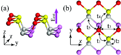
Figure 1: (color online). (a) Crystal structure of phosphorene, and (b) the top view of phosphorene, where the hopping parameters $t_{ij}$ of the tight-binding model are indicated. Circles of different colors correspond to atoms located in different planes within a single puckered layer.

Phosphorene has a characteristic puckered structure as shown in Fig.1, which leads to the two anisotropic in-plane directions. To specify the system size, we assume that the sample has totally $L_{y}$ zigzag chains with $L_{x}$ atomic sites on each zigzag chain Sheng2006 . The total number of sites in the sample is denoted as $N=L_{x}\times L_{y}$. In our numerical calculation, the system size is taken to be $N=96\times 48$, and the distance between nearest-neighbor sites is chosen as the unit of length. It have been shown that the calculated results do not depend on the system sizes, as long as the system lengths are reasonably large Ma2009 . The unit cell of phosphorene contains four phosphorus atoms, with two phosphorus atoms on the top layer and the other two on the bottom layer. When a magnetic field is applied perpendicular to the phosphorene film, the Hamiltonian can be written in the tight-binding form Rudenko2014 ,

$$H = \sum\limits_{\langle{ij}\rangle}t_{ij}e^{ia_{ij}}c_{i}^{\dagger}c_{j}+\sum\limits_{i}U_{i}c_{i}^{\dagger}c_{i}+H.c.+\sum\limits_{i}w_{i}c_{i}^{\dagger}c_{i}\ .$$ (1)

Here, the summation of $\langle{ij}\rangle$ runs over neighboring lattice sites, and $c_{i}^{\dagger}$ and $c_{i}$ are the creation and annihilation operators of electrons on site $i$. The hopping integrals $t_{ij}$ between site $i$ and its neighbours $j$ are described in Fig.1. The hopping integral $t_{1}$ corresponds to the connection along a zigzag chain in the upper or lower layer, and $t_{2}$ stands for the connection between a pair of zigzag chains in the upper and lower layers. $t_{3}$ is between the nearest-neighbour sites of a pair of zigzag chains in the upper or lower layer, and $t_{4}$ is between the next nearest-neighbour sites of a pair of zigzag chains in the upper and lower layers. $t_{5}$ is the hopping integral between two atoms on upper and lower zigzag chains that are farthest from each other. The values of these hopping integrals are $t_{1}=-1.220$ $eV$, $t_{2}=3.665$ $eV$, $t_{3}=-0.205$ $eV$, $t_{4}=-0.105$ $eV$, and $t_{5}=-0.055$ $eV$ Rudenko2014 . The magnetic flux per hexagon $\phi=\sum_{{\small{\mbox{\hexagon}}}}a_{ij}=\frac{2\pi}{M}$ is proportional to the strength of the applied magnetic field $B$, where $M$ is an integer and the lattice constant is taken to be unity. In the presence of a uniform perpendicular electric field, the electrostatic potentials of the top and bottom layers are set as $U_{top}=-U_{bottom}=\frac{1}{2}\Delta_{g}$ Ma2016 . For illustrative purpose, a relatively large potential difference $\Delta_{g}$=2$|t_{1}|$ is taken. The last term is the on-site random potential accounting for Anderson disorder, where $w_{i}$ is assumed to be uniformly distributed in the range $w_{i}\in[-W/2,W/2]$, with $W$ as the disorder strength Huo1992 ; Sheng97 .

In the linear response regime, the charge current in response to an electric field or a temperature gradient can be written as ${\bf J}={\hat{\sigma}}{\bf E}+{\hat{\alpha}}(-\nabla T)$, where ${\hat{\sigma}}$ and ${\hat{\alpha}}$ are the electrical and thermoelectric conductivity tensors, respectively. The electrical conductivity $\sigma_{ji}$ at zero temperature can be calculated by using the Kubo formula

$$\sigma_{ji}=\frac{ie^{2}\hbar}{A}\sum_{{\epsilon_{\alpha}}\neq{\epsilon_{\beta}}}\frac{f(\epsilon_{\alpha})-f(\epsilon_{\beta})}{\epsilon_{\alpha}-\epsilon_{\beta}}\frac{\langle\alpha\mid V_{j}\mid\beta\rangle\langle\beta\mid V_{i}\mid\alpha\rangle}{\epsilon_{\alpha}-\epsilon_{\beta}+i\eta},$$ (2)

Here, $\epsilon_{\alpha}$ and $\epsilon_{\beta}$ are the eigenenergies corresponding to the eigenstates $|\alpha\rangle$ and $|\beta\rangle$ of the system, respectively, which can be obtained through exact diagonalization of the Hamiltonian Eq. (1). $A$ is the area of the sample, and $f(\epsilon_{\alpha})$ and $f(\epsilon_{\beta})$ are the Fermi-Dirac distribution functions, defined as $f(x)=1/[e^{(x-E_{F})/k_{B}T}+1]$. $V_{j}$ and $V_{i}$ are the velocity operators, and $\eta$ is the positive infinitesimal, accounting for the finite broadening of the LLs. With tuning Fermi energy $E_{F}$, a series of integer-quantized Hall plateaus of $\sigma_{xy}$ appear, each one corresponding to $E_{F}$ moving in the gaps between two neighboring LLs.

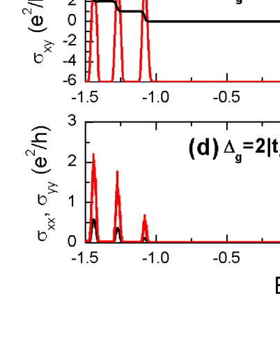
Figure 2: (color online). Calculated electron density of states, Hall conductivity $\sigma_{xy}$ and longitudinal conductivity $\sigma_{xx}$ ($\sigma_{yy}$) of phosphorene as functions of the Fermi energy at zero temperature. (a)-(b) $\Delta_{g}=0$, (c)-(d) $\Delta_{g}=2|t_{1}|$. The system size is taken to be $N=96\times 48$, magnetic flux $\phi=2\pi/48$, and disorder strength $W=0.5$. The positive infinitesimal $\eta$ is set to $10^{-3}eV$. Each data point is obtained by averaging over up to $2000$ disorder configurations.

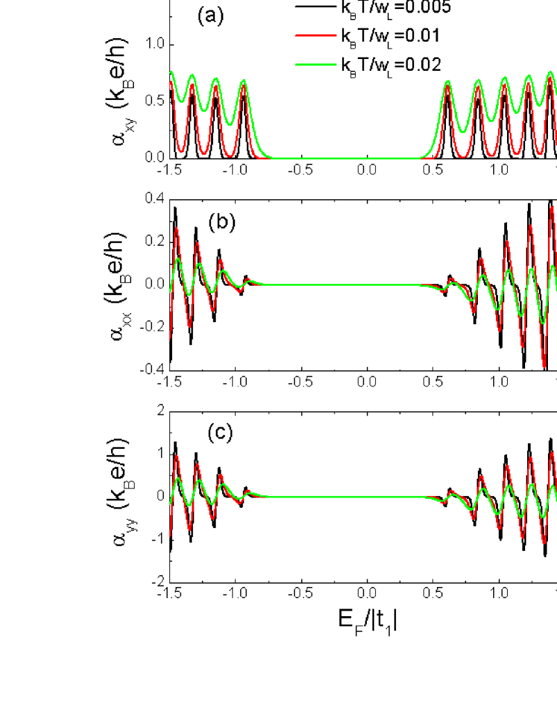
Figure 3: (color online). Thermoelectric conductivities at finite temperatures of phosphorene. (a)-(c)$\alpha_{xy}(E_{F},T)$, $\alpha_{xx}(E_{F},T)$ and $\alpha_{yy}(E_{F},T)$ as functions of the Fermi energy at different temperatures. (d)-(f) Comparison of the results from numerical calculations and from the generalized Mott relation for two characteristic temperatures, $k_{B}T/W_{L}=0.005$ and $k_{B}T/W_{L}=0.02$. Here, the asymmetric gap $W_{L}$ is equal to $W_{L}/|t_{1}|=1.548$, which is determined by the distance between two neighboring peaks of $\sigma_{xx}$ peaks around zero energy. The other parameters are chosen to be the same as in Fig.2.

We exactly diagonalize the model Hamiltonian in the presence of disorder Sheng97 , and obtain the transport coefficients by using the energy spectra and wave functions. In practice, we can first calculate the electrical conductivities $\sigma_{ji}$ at zero temperature, and then use the relation Jonson84

$$\sigma_{ji}(E_{F},T) = \int d\epsilon\,\sigma_{ji}(\epsilon)\left(-{\partial f(\epsilon)\over\partial\epsilon}\right),$$ (3)

$$\alpha_{ji}(E_{F},T) = {-1\over eT}\int d\epsilon\,\sigma_{ji}(\epsilon)(\epsilon-E_{F})\left(-{\partial f(\epsilon)\over\partial\epsilon}\right),$$ (4)

to obtain the electrical and thermoelectric conductivity at finite temperatures. At low temperatures, the second equation can be approximated as

$$\alpha_{ji}(E_{F},T)=-\frac{\pi^{2}k_{B}^{2}T}{3e}\left.\frac{d\sigma_{ji}(\epsilon,T)}{d\epsilon}\right|_{\epsilon=E_{F}},$$ (5)

which is the semiclassical Mott relation Jonson84 ; Oji84 . The validity of this relation will be examined for the present phosphorene system. The thermopower and Nernst signal can be calculated subsequently from footnote1

$$S_{xx} = {E_{x}\over\nabla_{x}T}=({\sigma_{yy}\alpha_{xx}+\sigma_{xy}\alpha_{xy}})/{D}$$ (6)

$$S_{yy} = {E_{y}\over\nabla_{y}T}=({\sigma_{xx}\alpha_{yy}+\sigma_{xy}\alpha_{xy}})/{D}$$ (7)

$$S_{xy} = {E_{x}\over\nabla_{y}T}=({\sigma_{yy}\alpha_{xy}-\sigma_{xy}\alpha_{yy}})/{D}$$ (8)

$$S_{yx} = {E_{y}\over\nabla_{x}T}=({-\sigma_{xx}\alpha_{xy}+\sigma_{xy}\alpha_{xx}})/{D},$$ (9)

with $D=\sigma_{xx}\sigma_{yy}+\sigma_{xy}^{2}$.

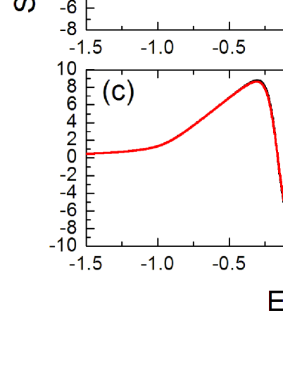
Figure 4: (color online). Calculated thermopower $S_{xx}$ and $S_{yy}$ as functions of the Fermi energy at three different temperatures in phosphorene.

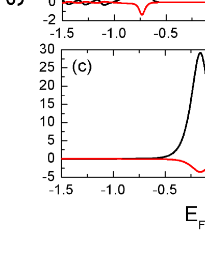
Figure 5: (color online). Calculated Nernst signal $S_{xy}$ and $S_{yx}$ as functions of the Fermi energy at three different temperatures in phosphorene.

III Results and Discussion

III.1 The electrical and thermoelectric transport

In Fig.2, we first show the electron density of states (DOS), the Hall conductivity $\sigma_{xy}$ and longitudinal conductivity $\sigma_{xx}$ ($\sigma_{yy}$) as functions of $E_{F}$ at zero temperature. In the presence of a magnetic field, the DOS is discrete, forming a series of LLs, as seen from the right part of Fig.2(a). We will call the LL just above $E_{F}=0$ as $n=1$ LL, that just below $E_{F}=0$ as $n=-1$ LL, and so on. Clearly, the central $n=0$ LL around $E_{F}$=0 is markedly absent. Moreover, all the LLs in the positive and negative regions are somewhat asymmetric in position, which can be attributed to the absence of particle-hole symmetry of the present band structure Ma2016 . The Hall conductivity is strictly quantized due to the quantized LLs. As can be seen from Fig.2(a), the Hall conductivity exhibits a sequence of plateaus at $\sigma_{xy}=\nu e^{2}/h$, where the filling factor $\nu=\pm kg_{s}$ with $k$ as an integer, and $g_{s}=1$ due to the lack of the valley degeneracy. With each additional LL being occupied, the total Hall conductivity is increased by $e^{2}/h$. This is an invariant as long as the states between the $n$-th and $(n-1)$-th LL are localized. Around zero energy point, a pronounced plateau with $\nu=0$ is found, which can only be understood as being due to the appearance of the bulk energy gap between the valence and conduction bands Rudenko2014 . Moreover, one can also see that the width of the $\nu=0$ plateaus is determined by the LL spacing between the two nearest levels. These results are somewhat similar to the conventional integer QHE found in the 2D semiconductor systems subject to a perpendicular magnetic field, but the conductivity plateaus in the conduction band and valence band are not antisymmetric in energy due to the asymmetric positions of the LLs. Our calculated results are in good agreement with the experimental observation of the QHE in black phosphorus Li2015 . In Figs.2(b), the longitudinal conductivity $\sigma_{xx}$ along the zigzag direction shows some pronounced peaks when the Fermi energy coincides with the LLs. According to the Kubo formula in Eq. (2), $\sigma_{xx}$ is proportional to $\sigma_{xx}\propto n{\partial f(\epsilon)\over\partial\epsilon}\delta(\epsilon-\epsilon_{n})$. As a result, $\sigma_{xx}$ displays a very similar structure to that of the DOS. In addition, the peak values of $\sigma_{xx}$ increase along with the increase of $E_{F}$ because of the larger transmission rate between the one-electron states $|\alpha\rangle$ and $|\beta\rangle$ with higher LLs index Zhou2015 ; Ando1974 ; Vasilopoulos2012 ; Zhou2014 . The results of the longitudinal conductivity along the armchair direction $\sigma_{yy}$ are qualitatively similar to those of $\sigma_{xx}$. Interestingly, the longitudinal conductivity exhibits an obvious anisotropic property, with the value along the zigzag direction much smaller than that along the armchair direction $\sigma_{xx}<\sigma_{yy}$. This anisotropic property is due to the anisotropic electronic structure Lv2014 ; Fei2014 . The band along the zigzag direction is much flatter than that along the armchair direction, which results in the much larger band effective mass and therefore much smaller carrier mobility and electrical conductivity in the zigzag direction.

When a bias voltage or a potential difference $\Delta_{g}$ is applied between the top and bottom layer of phosphorene, the Hall conductivity exhibits some interesting features. In Figs.2(c)-(d), we show the calculated DOS and electrical conductivity for a bias voltage $\Delta_{g}=2|t_{1}|$. As seen from Fig.2(c), the gap between the $n=\pm 1$ LLs is increased, which can only be understood as being due to the increase of the bulk energy gap between the valence and conduction bands. The Hall conductivity exhibits the same quantization rule as that of the unbiased phosphorene, while the width of the $\nu=0$ Hall plateau is enlarged due to the increase of the gap between the LLs. The longitudinal conductivity exhibits similar anisotropic behavior to that of the unbiased case, as shown in Figs.2(d).

Now we turn to study the thermoelectric transport coefficients of phosphorene. In Fig.3, we first plot the calculated thermoelectric conductivity at finite temperatures. Here, the temperature is defined by the ratio between $k_{B}T$ and $W_{L}$, where $W_{L}$ is the energy difference between the two nearest $\sigma_{xx}$ peaks around zero energy. As shown in Figs.3(a)-(c), the transverse thermoelectric conductivity $\alpha_{xy}$ displays a series of peaks, while the longitudinal thermoelectric conductivity ${\alpha_{xx}}$ (${\alpha_{yy}}$) oscillates and changes sign at the center of each LL. As seen from Fig.3(a), $\alpha_{xy}$ displays a pronounced valley with $\alpha_{xy}=0$ around zero energy at low temperatures. These are consistent with the presence of $\nu=0$ Hall plateau due to the lack of the valley degeneracy in phosphorene. Moreover, the positions of all the peaks in $\alpha_{xy}$ are asymmetric in energy due to the spectral asymmetry Ma2016 . In Figs.3(b) and (c), the longitudinal thermoelectric conductivity $\alpha_{xx}$($\alpha_{yy}$) also exhibits an obvious anisotropy, with the value along the zigzag direction much smaller than that along the armchair direction $\alpha_{xx}<\alpha_{yy}$. This is due to the anisotropic longitudinal conductivity. In Figs.3(d)-(f), we also compare the above results with those calculated from the semiclassical Mott relation given in Eq.(5). The Mott relation is found to remain valid only at low temperatures, indicating that the semiclassical Mott relation is asymptotically valid in Landau-quantized systems, as suggested in Ref. Jonson84, . With increasing temperature, its deviation will become more and more pronounced. However, if we take into account the finite-temperature values of electrical conductivity, the Mott relation still predicts the correct asymptotic behavior.

We further discuss some interesting features of the thermopower and Nernst signal in phosphorene using Eqs.(6)-(9), which can be directly observed in experiments by measuring the responsive electric fields. In Fig. 4, we first show the thermopower along the zigzag direction, $S_{xx}$, at different temperatures. As seen from Fig. 4(a), $S_{xx}$ exhibits a series of peaks at all the LLs. The largest peak values of $S_{xx}$ at $n=\pm 1$ LLs are found to be $\pm 6.6$ $k_{B}/e$ ($\pm 568.7$ $\mu V/K$) at $k_{B}T=0.005W_{L}$. With the increase of temperature, the peaks gradually rise and widen, their positions shifting towards $E_{F}=-0.16|t_{1}|$. As seen from Fig. 4(c), the peak values around $E_{F}=-0.16|t_{1}|$ increase to $\pm 8.8$ $k_{B}/e$ ($\pm 758.3$ $\mu V/K$) at $k_{B}T=0.05W_{L}$. We can see that there is only a very small difference between $S_{xx}$ and $S_{yy}$, and so the thermopower is nearly isotropic, which is qualitatively consistent with that obtained by Fei $et$ $al.$ Fei2014 ; Qin2014 ; Lv2014 .

In Fig. 5, we show the Nernst signals $S_{xy}$ and $S_{yx}$ at different temperatures. With the increase of temperature, the largest peak values of $S_{xy}$ and $S_{yx}$ increase, and the peak positions shift towards $E_{F}=-0.16|t_{1}|$. Interestingly, the Nernst signals exhibit remarkable anisotropic property over the whole temperature range. In addition to the opposite signs between $S_{xy}$ and $S_{yx}$, there is a big difference in magnitude between them. For example, at $k_{B}T=0.05W_{L}$, the peak value of $S_{xy}$ is $29.2$ $k_{B}/e$ (2516.2 $\mu V/K$), but the value of $S_{yx}$ is only $-3.6$ $k_{B}/e$ ($-310.2$ $\mu V/K$), as seen from Fig.5(c). This anisotropic origin can be understood by the following argument. Our calculation shows that in Eq. (8) or (9), the first term in the bracket is much greater than the second term, i.e., $\sigma_{yy}\alpha_{xy}\gg\sigma_{xy}\alpha_{yy}$ and $\sigma_{xx}\alpha_{xy}\gg\sigma_{xy}\alpha_{xx}$. As a result, we have $S_{xy}/S_{yx}\approx\sigma_{yy}/\sigma_{xx}$ from Eqs. (8) and (9). Due to the obvious anisotropy of the longitudinal conductivity $\sigma_{xx}<\sigma_{yy}$, we can conclude that the Nernst signal is also anisotropic, $S_{xy}>S_{yx}$.

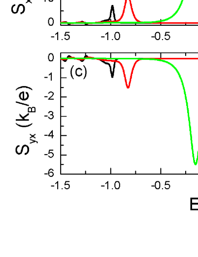
Figure 6: (color online). Calculated thermopower and Nernst signal in the presence of an applied bias voltage $\Delta_{g}$ of phosphorene at three different temperatures.

More interesting, when a bias voltage $\Delta_{g}$ is applied between the top and bottom layers of phosphorene, the peak values of thermopower and Nernst signal become large. As seen from Figs.6(a), the peak values of thermopower $S_{xx}$ increase to $\pm 9.9k_{B}/e$ ($\pm 853.1\mu V/K$), which are greater than those in the unbiased case. The enhanced thermopower is mainly due to the increase of the bulk energy gap between the valence and conduction bands. According to the definition of the thermopower, $S_{xx}$ is determined by the electron-transmission-weighted average value of the heat energy $E$-$E_{F}$. Due to the increase of the bulk energy gap in biased phosphorene, the electrons near the conduction band edge, which are responsible for the maximum thermopower, have a much larger $E$-$E_{F}$ compared to the case of unbiased phosphorene. This is similar to the situation in semiconducting armchair graphene nanoribbons ouyang2009 ; xing2009 ; hao2010 . On the other hand, the peak value of $S_{xy}$ increases to $39.4k_{B}/e$ (3395.1 $\mu V/K$), and the value of $S_{yx}$ increases to $-5.5$ $k_{B}/e$ ($-473.9$ $\mu V/K$). The enhanced thermopower and Nernst signal are very beneficial for the thermoelectric applications of phosphorene-based materials. It is known that a large thermopower does not necessarily lead to an enhanced power factor. On the contrary, a moderate thermopower combined with a suitable electrical conductivity may eventually result in a high power factor. The similar phenomenon has also been observed in experiments Zhao2014 .

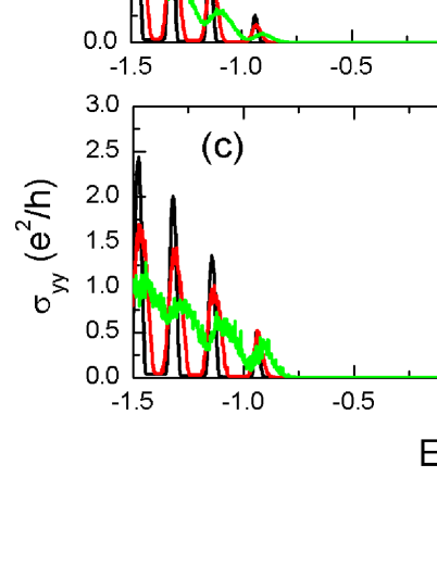
Figure 7: (color online). Calculated Hall conductivity $\sigma_{xy}$ and longitudinal conductivity $\sigma_{xx}$ ($\sigma_{yy}$) in units of $e^{2}/h$ as functions of the Fermi energy at zero temperature in phosphorene for three different disorder strengths.

III.2 Disorder effect on the electrical and thermoelectric transport

Now we study the effect of disorder on the electrical conductivity in phosphorene. In Fig.7, both Hall conductivity $\sigma_{xy}$ and longitudinal conductivity $\sigma_{xx}$ are shown as functions of $E_{F}$ for three different disorder strengths. As seen from Fig.7(a), the plateaus with $\nu=0,\pm 1,\pm 2$ and $\pm 3$ remain well quantized at $W=0.5$. With increasing $W$, the higher Hall plateaus (with larger $|\nu|$) are destroyed first because of the relatively small plateau widths. At $W=2.0$, only the $\nu=0$ QHE state remains robust. Clearly, after the destruction of the QHE states near the band edge, all the electron states become localized. Then the topological Chern numbers initially carried by these states will move towards band center in a similar manner to the case of graphene Sheng2006 . Thus the phase diagram indicates a float-up picture, in which the extended levels move towards band center with increasing disorder strength, causing higher plateaus to disappear first. As seen from Figs.7(b)and (c), the peaks of the calculated longitudinal conductivity $\sigma_{xx}$ are strongly broadened with increasing disorder strength.

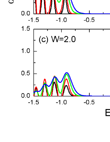
Figure 8: (color online). The transverse thermoelectric conductivity $\alpha_{xy}$ of phosphorene for three different disorder strengths. (a)$W=0.5$, (b)$W=1.0$ and (c)$W=2.0$. Here, the asymmetric gaps $W_{L}$ are equal to $W_{L}/|t_{1}|=1.851,1.824,$ and $1.755$, respectively.

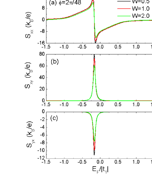
Figure 9: (color online). Calculated thermopower and Nernst signal of phosphorene for three different disorder strength at a fix temperature $k_{B}T=0.05W_{L}$. Here, $W_{L}$ is chosen as $W_{L}/|t_{1}|=1.8$. (a)-(b)$\phi=2\pi/48$, (c)-(d)$\phi=2\pi/24$.

We also investigate the disorder effect on the thermoelectric conductivity in phosphorene. In Fig.8, the transverse thermoelectric conductivity $\alpha_{xy}$ for three different disorder strengths $W=$0.5, 1.0 and 2.0 is shown. It is found that $\alpha_{xy}$ displays a series of peaks at the center of each LL. With increasing disorder strength from $W=0.5$ to $W=2.0$, the widths of peaks in $\alpha_{xy}$ increase. All the peaks will disappear around $W\sim 3.0$, which is caused by the merging of states with opposite Chern numbers at strong disorder Sheng2006 .

We finally investigate the disorder effect on the thermopower and Nernst signal in phosphorene. In Figs. 9(a)-(c), the calculated $S_{xx}$, $S_{xy}$ and $S_{yx}$ are plotted for different disorder strengths with magnetic flux $\phi=2\pi/48$. It is well known that when the magnetic field is absent, the thermopower is strongly affected by the disorder, and the peaks are suppressed even for small disorder Ma2016 . However, in the presence of the strong magnetic field, both thermopower and Nernst signal are robust to the disorder, due to the fact that the highly-degenerated LLs dominate transport processes. When the magnetic field is increased to $\phi=2\pi/24$, it is interesting to find that the peak heights of $S_{xx}$, $S_{xy}$ and $S_{yx}$ remain almost unchanged with increasing the disorder strength, as seen from Figs. 9(d)-(f). It means that, the stronger the magnetic field is, the more robust the thermopower and Nernst signal. In fact, a similar conclusion has been reached in the study of disorder effect in graphene nanoribbons xing2009 .

IV Summary

In summary, we have numerically investigated the electrical and thermoelectric transport properties of phosphorene in the presence of both a magnetic field and disorder. The quantized Hall conductivity is similar to that of a conventional 2DEG, but the positions of all the Hall plateaus shift to the left due to the spectral asymmetry. The thermoelectric conductivities and Nernst signal exhibit remarkable anisotropy, and the thermopower is nearly isotropic. Upon applying a bias voltage to phosphorene, the quantized Hall plateaus remain to follow the same sequence, but the width of $\nu=0$ plateau increases. It is interesting to find that the peak values of the thermopower and Nernst signal become larger compared to the unbiased case. We attribute the large magnitude of the thermopower to the increase of the bulk energy gap. Moreover, we also study the disorder effect on the electrical and thermoelectric transport in phosphorene. With increasing disorder strength, the Hall plateaus can be destroyed through the float-up of extended levels toward the band center and higher plateaus disappear first. The $\nu=0$ plateau is most robust against disorder scattering. In the presence of the strong magnetic field, both thermopower and Nernst signal are robust to the disorder, because of the existence of the quantized LLs. The stronger the magnetic field is, the more robust the thermopower and Nernst signal.

- (1) E. S. Reich, Nature 506, 19 (2014).
- (2) Likai Li, Fangyuan Yang, Guo Jun Ye, Zuocheng Zhang, Zengwei Zhu, Wen-Kai Lou, Liang Li, Kenji Watanabe, Takashi Taniguchi, Kai Chang, Yayu Wang, Xian Hui Chen and Yuanbo Zhang, Nature Nanotechnology, 11, 593 (2016).
- (3) L. Li, Y. Yu, G. J. Ye, Q. Ge, X. Ou, H. Wu, D. Feng, X. H. Chen, and Y. Zhang, Nature Nanotech. 9, 372 (2014).
- (4) H. Liu, A. T. Neal, Z. Zhu, D. Tománek and P. D. Ye, ACS Nano 8, 4033 (2014).
- (5) F. Xia, H. Wang, and Y. Jia, Nat. Commun. 5, 4458 (2014).
- (6) A. Castellanos-Gomez, L. Vicarelli, E. Prada, J. O. Island, K. L. Narasimha-Acharya, S. I. Blanter, D. J. Groenendijk, M. Buscema, G. A. Steele, J. V. Alvarez, H. W. Zandbergen, J. J. Palacios, and H. S. J. van der Zant, 2D Mater. 1, 025001 (2014).
- (7) S. P. Koenig, R. A. Doganov, H. Schmidt, A. H. Castro Neto, and B. zyilmaz, Appl. Phys. Lett. 104, 103106 (2014).
- (8) Moslem Zare, Babak Zare Rameshti, Farnood G. Ghamsari, and Reza Asgari, Phys. Rev. B 95, 045422 (2017).
- (9) J. Qiao, X. Kong, Z.X. Hu, F. Yang and W. Ji, Nat. Commun. 5, 4475 (2014).
- (10) R. Fei, A. Faghaninia, R. Soklaski, J. A. Yan, C. Lo, and L. Yang, Nano Lett, 14, 6393 (2014).
- (11) E. Flores, J. R. Ares, A. Castellanos-Gomez, M. Barawi, I. J. Ferrer, and C. Sánchez Appl. Phys. Lett. 106, 022102 (2015).
- (12) G. Qin, Q.B. Yan, Z. Qin, S.Y. Yue, H.J. Cui, Q.R. Zheng, and G. Su, Scientific Reports 4, 6946 (2014).
- (13) H. Y. Lv, W. J. Lu, D. F. Shao, and Y. P. Sun, Phys. Rev. B 90, 085433 (2014).
- (14) Satoru Konabe and Takahiro Yamamoto, Applied Physics Express 8, 015202 (2015).
- (15) Chang-Ran Wang, Wen-Sen Lu, Lei Hao, Wei-Li Lee, Ting-Kuo Lee, Feng Lin, I-Chun Cheng, and Jian-Zhang Chen, Phys. Rev. Lett. 107, 186602 (2011).
- (16) Lei Hao and T. K. Lee, Phys. Rev. B 81, 165445 (2010).
- (17) D. N. Sheng, L. Sheng, and Z. Y. Weng, Phys. Rev. B, 73, 233406 (2006).
- (18) R. Ma, L. Sheng, R. Shen, M. Liu, and D. N. Sheng, Phys. Rev. B, 80, 205101 (2009); R. Ma, L. Zhu, L. Sheng, M. Liu, and D. N. Sheng, Europhys. Lett., 87, 17009 (2009).
- (19) A. N. Rudenko and M. I. Katsnelson, Phys. Rev. B, 89, 201408 (2014).
- (20) R. Ma, H. Geng, W. Y. Deng, M. N. Chen, L. Sheng, and D. Y. Xing, Phys. Rev. B, 94, 125410 (2016).
- (21) Y. Huo and R. N. Bhatt, Phys. Rev. Lett. 68, 1375 (1992);
- (22) D. N. Sheng and Z. Y. Weng, Phys. Rev. Lett., 78, 318 (1997).
- (23) M. Jonson and S. M. Girvin, Phys. Rev. B, 29, 1939 (1984).
- (24) H. Oji, J. Phys. C, 17, 3059 (1984).
- (25) Different literatures may have a sign difference due to different conventions.
- (26) X. Y. Zhou, R. Zhang, J. P. Sun, Y. L. Zou, D. Zhang, W. K. Lou, F. Cheng, G. H. Zhou, F. Zhai and Kai Chang, Scientific Reports, 5, 12295 (2015).
- (27) Tsuneya Ando and Yasutada Uemura, J. Phys. Soc. Jpn. 36, 959 (1974).
- (28) P. M. Krstajić and P. Vasilopoulos, Phys. Rev. B 86, 115432 (2012).
- (29) Xiaoying Zhou, Yiman Liu, Ma Zhou, Dongsheng Tang and Guanghui Zhou, Journal of Physics: Condensed Matter, 26, 485008 (2014).
- (30) Y. Ouyang and J. Guo, Appl. Phys. Lett. 94, 263107 (2009).
- (31) Li-Dong Zhao, Shih-Han Lo, Yongsheng Zhang, Hui Sun, Gangjian Tan, Ctirad Uher, C. Wolverton, Vinayak P. Dravid and Mercouri G. Kanatzidis, Nature 508, 373 (2014).
- (32) Yanxia Xing, Qing-feng Sun, and J. Wang, Phys. Rev. B 80, 235411 (2009).