Reinforcement Learning for Bandit Neural Machine Translation with Simulated Human Feedback

Abstract

Machine translation is a natural candidate problem for reinforcement learning from human feedback: users provide quick, dirty ratings on candidate translations to guide a system to improve. Yet, current neural machine translation training focuses on expensive human-generated reference translations. We describe a reinforcement learning algorithm that improves neural machine translation systems from simulated human feedback. Our algorithm combines the advantage actor-critic algorithm Mnih et al. (2016) with the attention-based neural encoder-decoder architecture Luong et al. (2015). This algorithm (a) is well-designed for problems with a large action space and delayed rewards, (b) effectively optimizes traditional corpus-level machine translation metrics, and (c) is robust to skewed, high-variance, granular feedback modeled after actual human behaviors.

1 Introduction

Bandit structured prediction is the task of learning to solve complex joint prediction problems (like parsing or machine translation) under a very limited feedback model: a system must produce a single structured output (e.g., translation) and then the world reveals a score that measures how good or bad that output is, but provides neither a “correct” output nor feedback on any other possible output Chang et al. (2015); Sokolov et al. (2015). Because of the extreme sparsity of this feedback, a common experimental setup is that one pre-trains a good-but-not-great “reference” system based on whatever labeled data is available, and then seeks to improve it over time using this bandit feedback. A common motivation for this problem setting is cost. In the case of translation, bilingual “experts” can read a source sentence and a possible translation, and can much more quickly provide a rating of that translation than they can produce a full translation on their own. Furthermore, one can often collect even less expensive ratings from “non-experts” who may or may not be bilingual Hu et al. (2014). Breaking this reliance on expensive data could unlock previously ignored languages and speed development of broad-coverage machine translation systems.

All work on bandit structured prediction we know makes an important simplifying assumption: the score provided by the world is exactly the score the system must optimize (§ 2). In the case of parsing, the score is attachment score; in the case of machine translation, the score is (sentence-level) Bleu. While this simplifying assumption has been incredibly useful in building algorithms, it is highly unrealistic. Any time we want to optimize a system by collecting user feedback, we must take into account:

1. The metric we care about (e.g., expert ratings) may not correlate perfectly with the measure that the reference system was trained on (e.g., Bleu or log likelihood);

2. Human judgments might be more granular than traditional continuous metrics (e.g., thumbs up vs. thumbs down);

3. Human feedback have high variance (e.g., different raters might give different responses given the same system output);

4. Human feedback might be substantially skewed (e.g., a rater may think all system outputs are poor).

Our first contribution is a strategy to simulate expert and non-expert ratings to evaluate the robustness of bandit structured prediction algorithms in general, in a more realistic environment (§ 4). We construct a family of perturbations to capture three attributes: granularity, variance, and skew. We apply these perturbations on automatically generated scores to simulate noisy human ratings. To make our simulated ratings as realistic as possible, we study recent human evaluation data Graham et al. (2017) and fit models to match the noise profiles in actual human ratings (§ 4.2).

Our second contribution is a reinforcement learning solution to bandit structured prediction and a study of its robustness to these simulated human ratings (§ 3). We combine an encoder-decoder architecture of machine translation Luong et al. (2015) with the advantage actor-critic algorithm Mnih et al. (2016), yielding an approach that is simple to implement but works on low-resource bandit machine translation. Even with substantially restricted granularity, with high variance feedback, or with skewed rewards, this combination improves pre-trained models (§ 6). In particular, under realistic settings of our noise parameters, the algorithm’s online reward and final held-out accuracies do not significantly degrade from a noise-free setting.

2 Bandit Machine Translation

The bandit structured prediction problem Chang et al. (2015); Sokolov et al. (2015) is an extension of the contextual bandits problem Kakade et al. (2008); Langford and Zhang (2008) to structured prediction. Bandit structured prediction operates over time $i=1\dots K$ as:

1. World reveals context $\boldsymbol{x}^{(i)}$

2. Algorithm predicts structured output $\hat{\boldsymbol{y}}^{(i)}$

3. World reveals reward $R\left(\hat{\boldsymbol{y}}^{(i)},\boldsymbol{x}^{(i)}\right)$

We consider the problem of learning to translate from human ratings in a bandit structured prediction framework. In each round, a translation model receives a source sentence $\boldsymbol{x}^{(i)}$, produces a translation $\hat{\boldsymbol{y}}^{(i)}$, and receives a rating $R\left(\hat{\boldsymbol{y}}^{(i)},\boldsymbol{x}^{(i)}\right)$ from a human that reflects the quality of the translation. We seek an algorithm that achieves high reward over $K$ rounds (high cumulative reward). The challenge is that even though the model knows how good the translation is, it knows neither where its mistakes are nor what the “correct” translation looks like. It must balance exploration (finding new good predictions) with exploitation (producing predictions it already knows are good). This is especially difficult in a task like machine translation, where, for a twenty token sentence with a vocabulary size of $50k$, there are approximately $10^{94}$ possible outputs, of which the algorithm gets to test exactly one.

Figure 1: A translation rating interface provided by Facebook. Users see a sentence followed by its machined-generated translation and can give ratings from one to five stars.

Despite these challenges, learning from non-expert ratings is desirable. In real-world scenarios, non-expert ratings are easy to collect but other stronger forms of feedback are prohibitively expensive. Platforms that offer translations can get quick feedback “for free” from their users to improve their systems (Figure 1). Even in a setting in which annotators are paid, it is much less expensive to ask a bilingual speaker to provide a rating of a proposed translation than it is to pay a professional translator to produce one from scratch.

3 Effective Algorithm for Bandit MT

This section describes the neural machine translation architecture of our system (§ 3.1). We formulate bandit neural machine translation as a reinforcement learning problem (§ 3.2) and discuss why standard actor-critic algorithms struggle with this problem (§ 3.3). Finally, we describe a more effective training approach based on the advantage actor-critic algorithm (§ 3.4).

3.1 Neural machine translation

Our neural machine translation (NMT) model is a neural encoder-decoder that directly computes the probability of translating a target sentence $\boldsymbol{y}=(y_{1},\cdots,y_{m})$ from source sentence $\boldsymbol{x}$:

$$P_{\boldsymbol{\theta}}(\boldsymbol{y}\mid\boldsymbol{x})=\prod_{t=1}^{m}P_{\boldsymbol{\theta}}(y_{t}\mid\boldsymbol{y}_{<t},\boldsymbol{x})$$ (1)

where $P_{\boldsymbol{\theta}}(y_{t}\mid\boldsymbol{y}_{<t},\boldsymbol{x})$ is the probability of outputting the next word $y_{t}$ at time step $t$ given a translation prefix $\boldsymbol{y}_{<t}$ and a source sentence $\boldsymbol{x}$.

We use an encoder-decoder NMT architecture with global attention Luong et al. (2015), where both the encoder and decoder are recurrent neural networks (RNN) (see Appendix A for a more detailed description). These models are normally trained by supervised learning, but as reference translations are not available in our setting, we use reinforcement learning methods, which only require numerical feedback to function.

3.2 Bandit NMT as Reinforcement Learning

NMT generating process can be viewed as a Markov decision process on a continuous state space. The states are the hidden vectors $\boldsymbol{h}_{t}^{dec}$ generated by the decoder. The action space is the target language’s vocabulary.

To generate a translation from a source sentence $\boldsymbol{x}$, an NMT model starts at an initial state $\boldsymbol{h}_{0}^{dec}$: a representation of $\boldsymbol{x}$ computed by the encoder. At time step $t$, the model decides the next action to take by defining a stochastic policy $P_{\boldsymbol{\theta}}(y_{t}\mid\boldsymbol{y}_{<t},\boldsymbol{x})$, which is directly parametrized by the parameters $\boldsymbol{\theta}$ of the model. This policy takes the current state $\boldsymbol{h}_{t-1}^{dec}$ as input and produces a probability distribution over all actions (target vocabulary words). The next action $\hat{y}_{t}$ is chosen by taking $\arg\max$ or sampling from this distribution. The model computes the next state $\boldsymbol{h}_{t}^{dec}$ by updating the current state $\boldsymbol{h}_{t-1}^{dec}$ by the action taken $\hat{y}_{t}$.

The objective of bandit NMT is to find a policy that maximizes the expected reward of translations sampled from the model’s policy:

$$\max_{\boldsymbol{\theta}}\mathcal{L}_{pg}(\boldsymbol{\theta})=\max_{\boldsymbol{\theta}}\mathbb{E}_{\begin{subarray}{c}\boldsymbol{x}\sim D_{\textrm{tr}}\\ \hat{\boldsymbol{y}}\sim P_{\boldsymbol{\theta}}(\cdot\mid\boldsymbol{x})\end{subarray}}\Big{[}R(\hat{\boldsymbol{y}},\boldsymbol{x})\Big{]}$$ (2)

where $D_{tr}$ is the training set and $R$ is the reward function (the rater). We optimize this objective function with policy gradient methods. For a fixed $\boldsymbol{x}$, the gradient of the objective in Eq 2 is:

$$\nabla_{\boldsymbol{\theta}}\mathcal{L}_{pg}(\boldsymbol{\theta})=\mathbb{E}_{\hat{\boldsymbol{y}}\sim P_{\boldsymbol{\theta}}(\cdot)}\left[R(\hat{\boldsymbol{y}})\nabla_{\boldsymbol{\theta}}\log P_{\boldsymbol{\theta}}(\hat{\boldsymbol{y}})\right]$$ (3)

$$=\mathbb{E}_{\begin{subarray}{c}\hat{\boldsymbol{y}}\sim P_{\boldsymbol{\theta}}(\cdot)\end{subarray}}\Big{[}\sum_{t=1}^{m}\sum_{y_{t}}Q(\hat{\boldsymbol{y}}_{<t},\hat{y}_{t})\nabla_{\boldsymbol{\theta}}P_{\boldsymbol{\theta}}(\hat{y}_{t}\mid\hat{\boldsymbol{y}}_{<t})\Big{]}$$

where $Q(\hat{\boldsymbol{y}}_{<t},\hat{y}_{t})$ is the expected future reward of $\hat{y}_{t}$ given the current prefix $\hat{\boldsymbol{y}}_{<t}$, then continuing sampling from $P_{\boldsymbol{\theta}}$ to complete the translation:

$$Q(\hat{\boldsymbol{y}}_{<t},\hat{y}_{t}) =\mathbb{E}_{\hat{\boldsymbol{y}}^{\prime}\sim P_{\boldsymbol{\theta}}(\cdot\mid\boldsymbol{x})}\left[\tilde{R}(\hat{\boldsymbol{y}}^{\prime},\boldsymbol{x})\right]$$ (4)

$$\textrm{with }\tilde{R}(\hat{\boldsymbol{y}}^{\prime},\boldsymbol{x}) \equiv R(\hat{\boldsymbol{y}}^{\prime},\boldsymbol{x})\mathbbm{1}\left\{\hat{\boldsymbol{y}}^{\prime}_{<t}=\hat{\boldsymbol{y}}_{<t},\hat{y}^{\prime}_{t}=\hat{y}_{t}\right\}$$

$\mathbbm{1}\{\cdot\}$ is the indicator function, which returns 1 if the logic inside the bracket is true and returns 0 otherwise.

The gradient in Eq 3 requires rating all possible translations, which is not feasible in bandit NMT. Naïve Monte Carlo reinforcement learning methods such as REINFORCE Williams (1992) estimates $Q$ values by sample means but yields very high variance when the action space is large, leading to training instability.

3.3 Why are actor-critic algorithms not effective for bandit NMT?

Reinforcement learning methods that rely on function approximation are preferred when tackling bandit structured prediction with a large action space because they can capture similarities between structures and generalize to unseen regions of the structure space. The actor-critic algorithm Konda and Tsitsiklis uses function approximation to directly model the $Q$ function, called the critic model. In our early attempts on bandit NMT, we adapted the actor-critic algorithm for NMT in Bahdanau et al. (2017), which employs the algorithm in a supervised learning setting. Specifically, while an encoder-decoder critic model $Q_{\boldsymbol{\omega}}$ as a substitute for the true $Q$ function in Eq 3 enables taking the full sum inside the expectation (because the critic model can be queried with any state-action pair), we are unable to obtain reasonable results with this approach.

Nevertheless, insights into why this approach fails on our problem explains the effectiveness of the approach discussed in the next section. There are two properties in Bahdanau et al. (2017) that our problem lacks but are key elements for a successful actor-critic. The first is access to reference translations: while the critic model is able to observe reference translations during training in their setting, bandit NMT assumes those are never available. The second is per-step rewards: while the reward function in their setting is known and can be exploited to compute immediate rewards after taking each action, in bandit NMT, the actor-critic algorithm struggles with credit assignment because it only receives reward when a translation is completed. Bahdanau et al. (2017) report that the algorithm degrades if rewards are delayed until the end, consistent with our observations.

With an enormous action space of bandit NMT, approximating gradients with the $Q$ critic model induces biases and potentially drives the model to wrong optima. Values of rarely taken actions are often overestimated without an explicit constraint between $Q$ values of actions (e.g., a sum-to-one constraint). Bahdanau et al. (2017) add an ad-hoc regularization term to the loss function to mitigate this issue and further stablizes the algorithm with a delay update scheme, but at the same time introduces extra tuning hyper-parameters.

3.4 Advantage Actor-Critic for Bandit NMT

We follow the approach of advantage actor-critic (Mnih et al., 2016, A2C) and combine it with the neural encoder-decoder architecture. The resulting algorithm—which we call NED-A2C—approximates the gradient in Eq 3 by a single sample $\hat{\boldsymbol{y}}\sim P(\cdot\mid\hat{\boldsymbol{x}})$ and centers the reward $R(\hat{\boldsymbol{y}})$ using the state-specific expected future reward $V(\hat{\boldsymbol{y}}_{<t})$ to reduce variance:

$$\nabla_{\boldsymbol{\theta}}\mathcal{L}_{pg}(\boldsymbol{\theta}) \approx\sum_{t=1}^{m}\bar{R}_{t}(\hat{\boldsymbol{y}})\nabla_{\boldsymbol{\theta}}\log P_{\boldsymbol{\theta}}(\hat{y}_{t}\mid\hat{\boldsymbol{y}}_{<t})$$ (5)

$$\textrm{with }\bar{R}_{t}(\hat{\boldsymbol{y}}) \equiv R(\hat{\boldsymbol{y}})-V(\hat{\boldsymbol{y}}_{<t})$$

$$V(\hat{\boldsymbol{y}}_{<t}) \equiv\mathbb{E}_{\hat{y}^{\prime}_{t}\sim P(\cdot\mid\hat{\boldsymbol{y}}_{<t})}\left[Q(\hat{\boldsymbol{y}}_{<t},\hat{y}^{\prime}_{t})\right]$$

We train a separate attention-based encoder-decoder model $V_{\boldsymbol{\omega}}$ to estimate $V$ values. This model encodes a source sentence $\boldsymbol{x}$ and decodes a sampled translation $\hat{\boldsymbol{y}}$. At time step $t$, it computes $V_{\boldsymbol{\omega}}(\hat{\boldsymbol{y}}_{<t},\boldsymbol{x})=\boldsymbol{w}^{\top}\boldsymbol{h}_{t}^{crt}$, where $\boldsymbol{h}^{crt}_{t}$ is the current decoder’s hidden vector and $\boldsymbol{w}$ is a learned weight vector. The critic model minimizes the MSE between its estimates and the true values:

$$\mathcal{L}_{crt}(\boldsymbol{\omega}) =\mathbb{E}_{\begin{subarray}{c}\boldsymbol{x}\sim D_{\textrm{tr}}\\ \hat{\boldsymbol{y}}\sim P_{\boldsymbol{\theta}}(\cdot\mid\boldsymbol{x})\end{subarray}}\left[\sum_{t=1}^{m}L_{t}(\hat{\boldsymbol{y}},\boldsymbol{x})\right]$$ (6)

$$\textrm{with }L_{t}(\hat{\boldsymbol{y}},\boldsymbol{x}) \equiv\left[V_{\boldsymbol{\omega}}(\hat{\boldsymbol{y}}_{<t},\boldsymbol{x})-R(\hat{\boldsymbol{y}},\boldsymbol{x})\right]^{2}.$$

We use a gradient approximation to update $\boldsymbol{\omega}$ for a fixed $\boldsymbol{x}$ and $\hat{\boldsymbol{y}}\sim P(\cdot\mid\hat{\boldsymbol{x}})$:

$$\nabla_{\boldsymbol{\omega}}\mathcal{L}_{crt}(\boldsymbol{\omega})\approx\sum_{t=1}^{m}\left[V_{\boldsymbol{\omega}}(\hat{\boldsymbol{y}}_{<t})-R(\hat{\boldsymbol{y}})\right]\nabla_{\boldsymbol{\omega}}V_{\boldsymbol{\omega}}(\hat{\boldsymbol{y}}_{<t})$$ (7)

NED-A2C is better suited for problems with a large action space and has other advantages over actor-critic. For large action spaces, approximating gradients using the $V$ critic model induces lower biases than using the $Q$ critic model. As implied by its definition, the $V$ model is robust to biases incurred by rarely taken actions since rewards of those actions are weighted by very small probabilities in the expectation. In addition, the $V$ model has a much smaller number of parameters and thus is more sample-efficient and more stable to train than the $Q$ model. These attractive properties were not studied in A2C’s original paper Mnih et al. (2016).

Algorithm 1 The NED-A2C algorithm for bandit NMT.

1:  for $i=1\cdots K$ do

2:     receive a source sentence $\boldsymbol{x}^{(i)}$

3:     sample a translation: $\hat{\boldsymbol{y}}^{(i)}\sim P_{\boldsymbol{\theta}}(\cdot\mid\boldsymbol{x}^{(i)})$

4:     receive reward $R(\hat{\boldsymbol{y}}^{(i)},\boldsymbol{x}^{(i)})$

5:     update the NMT model using Eq 5.

6:     update the critic model using Eq 7.

7:  end for

Algorithm 1 summarizes NED-A2C for bandit NMT. For each $\boldsymbol{x}$, we draw a single sample $\hat{\boldsymbol{y}}$ from the NMT model, which is used for both estimating gradients of the NMT model and the critic model. We run this algorithm with mini-batches of $\boldsymbol{x}$ and aggregate gradients over all $\boldsymbol{x}$ in a mini-batch for each update. Although our focus is on bandit NMT, this algorithm naturally works with any bandit structured prediction problem.

4 Modeling Imperfect Ratings

Our goal is to establish the feasibility of using real human feedback to optimize a machine translation system, in a setting where one can collect expert feedback as well as a setting in which one only collects non-expert feedback. In all cases, we consider the expert feedback to be the “gold standard” that we wish to optimize. To establish the feasibility of driving learning from human feedback without doing a full, costly user study, we begin with a simulation study. The key aspects (Figure 2) of human feedback we capture are: (a) mismatch between training objective and feedback-maximizing objective, (b) human ratings typically are binned (§ 4.1), (c) individual human ratings have high variance (§ 4.2), and (d) non-expert ratings can be skewed with respect to expert ratings (§ 4.3).

In our simulated study, we begin by modeling gold standard human ratings using add-one-smoothed sentence-level Bleu Chen and Cherry (2014). Our evaluation criteria, therefore, is average sentence-Bleu over the run of our algorithm. However, in any realistic scenario, human feedback will vary from its average, and so the reward that our algorithm receives will be a perturbed variant of sentence-Bleu. In particular, if the sentence-Bleu score is $s\in[0,1]$, the algorithm will only observe $s^{\prime}\sim\textrm{pert}(s)$, where pert is a perturbation distribution. Because our reference machine translation system is pre-trained using log-likelihood, there is already an (a) mismatch between training objective and feedback, so we focus on (b-d) below.

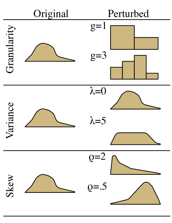
Figure 2: Examples of how our perturbation functions change the “true” feedback distribution (left) to ones that better capture features found in human feedback (right).

4.1 Humans Provide Granular Feedback

When collecting human feedback, it is often more effective to collect discrete binned scores. A classic example is the Likert scale for human agreement Likert (1932) or star ratings for product reviews. Insisting that human judges provide continuous values (or feedback at too fine a granularity) can demotivate raters without improving rating quality Preston and Colman (2000).

To model granular feedback, we use a simple rounding procedure. Given an integer parameter $g$ for degree of granularity, we define:

$$\textrm{pert}^{\textrm{gran}}(s;g) =\frac{1}{g}\textrm{round}(gs)$$ (8)

This perturbation function divides the range of possible outputs into $g+1$ bins. For example, for $g=5$, we obtain bins $[0,0.1)$, $[0.1,0.3)$, $[0.3,0.5)$, $[0.5,0.7)$, $[0.7,0.9)$ and $[0.9,1.0]$. Since most sentence-Bleu scores are much closer to zero than to one, many of the larger bins are frequently vacant.

4.2 Experts Have High Variance

Human feedback has high variance around its expected value. A natural goal for a variance model of human annotators is to simulate—as closely as possible—how human raters actually perform. We use human evaluation data recently collected as part of the WMT shared task Graham et al. (2017). The data consist of 7200 sentences multiply annotated by giving non-expert annotators on Amazon Mechanical Turk a reference sentence and a single system translation, and asking the raters to judge the adequacy of the translation.

From these data, we treat the average human rating as the ground truth and consider how individual human ratings vary around that mean. To visualize these results with kernel density estimates (standard normal kernels) of the standard deviation. Figure 3 shows the mean rating (x-axis) and the deviation of the human ratings (y-axis) at each mean.As expected, the standard deviation is small at the extremes and large in the middle (this is a bounded interval), with a fairly large range in the middle: a translation whose average score is $50$ can get human evaluation scores anywhere between $20$ and $80$ with high probability. We use a linear approximation to define our variance-based perturbation function as a Gaussian distribution, which is parameterized by a scale $\lambda$ that grows or shrinks the variances (when $\lambda=1$ this exactly matches the variance in the plot).

$$\textrm{pert}^{\textrm{var}}(s;\lambda) =\textrm{Nor}\left(s,\lambda\sigma(s)^{2}\right)$$ (9)

$$\sigma(s) =\left\{\begin{array}[]{ll}~{}~{}~{}0.64s-0.02&\textrm{if }s<50\\ -0.67s+67.0&\textrm{otherwise}\end{array}\right.$$ (12)

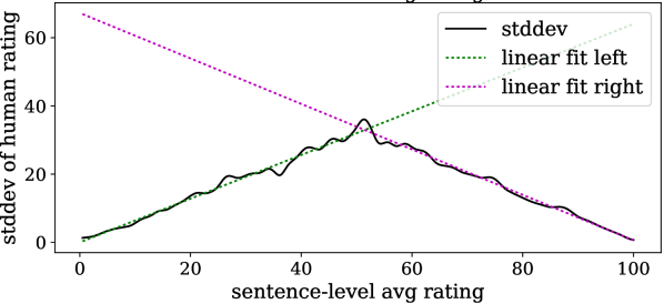
Figure 3: Average rating (x-axis) versus a kernel density estimate of the variance of human ratings around that mean, with linear fits. Human scores vary more around middling judgments than extreme judgments.

4.3 Non-Experts are Skewed from Experts

The preceding two noise models assume that the reward closely models the value we want to optimize (has the same mean). This may not be the case with non-expert ratings. Non-expert raters are skewed both for reinforcement learning Thomaz et al. (2006); Thomaz and Breazeal (2008); Loftin et al. (2014) and recommender systems Herlocker et al. (2000); Adomavicius and Zhang (2012), but are typically bimodal: some are harsh (typically provide very low scores, even for “okay” outputs) and some are motivational (providing high scores for “okay” outputs).

We can model both harsh and motivations raters with a simple deterministic skew perturbation function, parametrized by a scalar $\rho\in[0,\infty)$:

$$\textrm{pert}^{\textrm{skew}}(s;\rho) =s^{\rho}$$ (13)

For $\rho>1$, the rater is harsh; for $\rho<1$, the rater is motivational.

5 Experimental Setup

	De-En	Zh-En
Supervised training	186K	190K
Bandit training	167K	165K
Development	7.7K	7.9K
Test	9.1K	7.4K

Table 1: Sentence counts in data sets.

We choose two language pairs from different language families with different typological properties: German-to-English and (De-En) and Chinese-to-English (Zh-En). We use parallel transcriptions of TED talks for these pairs of languages from the machine translation track of the IWSLT 2014 and 2015 Cettolo et al. (2014, 2015, 2012). For each language pair, we split its data into four sets for supervised training, bandit training, development and testing (Table 1). For English and German, we tokenize and clean sentences using Moses Koehn et al. (2007). For Chinese, we use the Stanford Chinese word segmenter Chang et al. (2008) to segment sentences and tokenize. We remove all sentences with length greater than 50, resulting in an average sentence length of 18. We use IWSLT 2015 data for supervised training and development, IWSLT 2014 data for bandit training and previous years’ development and evaluation data for testing.

5.1 Evaluation Framework

For each task, we first use the supervised training set to pre-train a reference NMT model using supervised learning. On the same training set, we also pre-train the critic model with translations sampled from the pre-trained NMT model. Next, we enter a bandit learning mode where our models only observe the source sentences of the bandit training set. Unless specified differently, we train the NMT models with NED-A2C for one pass over the bandit training set. If a perturbation function is applied to Per-Sentence Bleu scores, it is only applied in this stage, not in the pre-training stage.

We measure the improvement $\Delta S$ of an evaluation metric $S$ due to bandit training: $\Delta S=S_{A2C}-S_{ref}$, where $S_{ref}$ is the metric computed on the reference models and $S_{A2C}$ is the metric computed on models trained with NED-A2C. Our primary interest is Per-Sentence Bleu: average sentence-level Bleu of translations that are sampled and scored during the bandit learning pass. This metric represents average expert ratings, which we want to optimize for in real-world scenarios. We also measure Heldout Bleu: corpus-level Bleu on an unseen test set, where translations are greedily decoded by the NMT models. This shows how much our method improves translation quality, since corpus-level Bleu correlates better with human judgments than sentence-level Bleu.

Because of randomness due to both the random sampling in the model for “exploration” as well as the randomness in the reward function, we repeat each experiment five times and report the mean results with 95% confidence intervals.

5.2 Model configuration

Both the NMT model and the critic model are encoder-decoder models with global attention Luong et al. (2015). The encoder and the decoder are unidirectional single-layer LSTMs. They have the same word embedding size and LSTM hidden size of 500. The source and target vocabulary sizes are both 50K. We do not use dropout in our experiments. We train our models by the Adam optimizer Kingma and Ba (2015) with $\beta_{1}=0.9,\beta_{2}=0.999$ and a batch size of 64. For Adam’s $\alpha$ hyperparameter, we use $10^{-3}$ during pre-training and $10^{-4}$ during bandit learning (for both the NMT model and the critic model). During pre-training, starting from the fifth pass, we decay $\alpha$ by a factor of 0.5 when perplexity on the development set increases. The NMT model reaches its highest corpus-level Bleu on the development set after ten passes through the supervised training data, while the critic model’s training error stabilizes after five passes. The training speed is 18s/batch for supervised pre-training and 41s/batch for training with the NED-A2C algorithm.

6 Results and Analysis

In this section, we describe the results of our experiments, broken into the following questions: how NED-A2C improves reference models (§ 6.1); the effect the three perturbation functions have on the algorithm (§ 6.2); and whether the algorithm improves a corpus-level metric that corresponds well with human judgments (§ 6.3).

6.1 Effectiveness of NED-A2C under Un-perturbed Bandit Feedback

	De-En			Zh-En
	Reference	$\Delta_{sup}$	$\Delta_{A2C}$	Reference	$\Delta_{sup}$	$\Delta_{A2C}$
Fully pre-trained reference model
Per-Sentence Bleu	38.26 $\pm$ 0.02	0.07 $\pm$ 0.05	2.82 $\pm$ 0.03	32.79 $\pm$ 0.01	0.36 $\pm$ 0.05	1.08 $\pm$ 0.03
Heldout Bleu	24.94 $\pm$ 0.00	1.48 $\pm$ 0.00	1.82 $\pm$ 0.08	13.73 $\pm$ 0.00	1.18 $\pm$ 0.00	0.86 $\pm$ 0.11
Weakly pre-trained reference model
Per-Sentence Bleu	19.15 $\pm$ 0.01	2.94 $\pm$ 0.02	7.07 $\pm$ 0.06	14.77 $\pm$ 0.01	1.11 $\pm$ 0.02	3.60 $\pm$ 0.04
Heldout Bleu	19.63 $\pm$ 0.00	3.94 $\pm$ 0.00	1.61 $\pm$ 0.17	9.34 $\pm$ 0.00	2.31 $\pm$ 0.00	0.92 $\pm$ 0.13

Table 2: Translation scores and improvements based on a single round of un-perturbed bandit feedback. Per-Sentence Bleu and Heldout Bleu are not comparable: the former is sentence-Bleu, the latter is corpus-Bleu.

We evaluate our method in an ideal setting where un-perturbed Per-Sentence Bleu simulates ratings during both training and evaluation (Table 2).

Single round of feedback.

In this setting, our models only observe each source sentence once and before producing its translation. On both De-En and Zh-En, NED-A2C improves Per-Sentence Bleu of reference models after only a single pass (+2.82 and +1.08 respectively).

Poor initialization.

Policy gradient algorithms have difficulty improving from poor initializations, especially on problems with a large action space, because they use model-based exploration, which is ineffective when most actions have equal probabilities Bahdanau et al. (2017); Ranzato et al. (2016). To see whether NED-A2C has this problem, we repeat the experiment with the same setup but with reference models pre-trained for only a single pass. Surprisingly, NED-A2C is highly effective at improving these poorly trained models (+7.07 on De-En and +3.60 on Zh-En in Per-Sentence Bleu).

Comparisons with supervised learning.

To further demonstrate the effectiveness of NED-A2C, we compare it with training the reference models with supervised learning for a single pass on the bandit training set. Surprisingly, observing ground-truth translations barely improves the models in Per-Sentence Bleu when they are fully trained (less than +0.4 on both tasks). A possible explanation is that the models have already reached full capacity and do not benefit from more examples. NED-A2C further enhances the models because it eliminates the mismatch between the supervised training objective and the evaluation objective. On weakly trained reference models, NED-A2C also significantly outperforms supervised learning ($\Delta$Per-Sentence Bleu of NED-A2C is over three times as large as those of supervised learning).

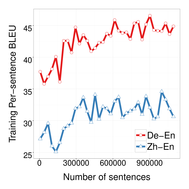
Figure 4: Learning curves of models trained with NED-A2C for five epochs.

Multiple rounds of feedback.

We examine if NED-A2C can improve the models even further with multiple rounds of feedback. With supervised learning, the models can memorize the reference translations but, in this case, the models have to be able to exploit and explore effectively. We train the models with NED-A2C for five passes and observe a much more significant $\Delta$Per-Sentence Bleu than training for a single pass in both pairs of language (+6.73 on De-En and +4.56 on Zh-En) (Figure 4).

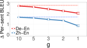
(a) Granularity

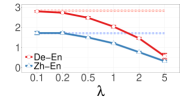
(b) Variance

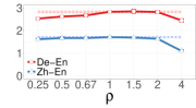
(c) Skew

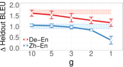
(d) Granularity

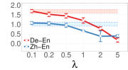
(e) Variance

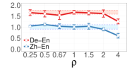
(f) Skew

Figure 5: Performance gains of NMT models trained with NED-A2C in Per-Sentence Bleu (top row) and in Heldout Bleu (bottom row) under various degrees of granularity, variance, and skew of scores. Performance gains of models trained with un-perturbed scores are within the shaded regions.

6.2 Effect of Perturbed Bandit Feedback

We apply perturbation functions defined in § 4.1 to Per-Sentence Bleu scores and use the perturbed scores as rewards during bandit training (Figure 5).

Granular Rewards.

We discretize raw Per-Sentence Bleu scores using $\textrm{pert}^{gran}(s;g)$ (§ 4.1). We vary $g$ from one to ten (number of bins varies from two to eleven). Compared to continuous rewards, for both pairs of languages, $\Delta$Per-Sentence Bleu is not affected with $g$ at least five (at least six bins). As granularity decreases, $\Delta$Per-Sentence Bleu monotonically degrades. However, even when $g=1$ (scores are either 0 or 1), the models still improve by at least a point.

High-variance Rewards.

We simulate noisy rewards using the model of human rating variance $\textrm{pert}^{var}(s;\lambda)$ (§ 4.2) with $\lambda\in\{0.1,0.2,0.5,1,2,5\}$. Our models can withstand an amount of about 20% the variance in our human eval data without dropping in $\Delta$Per-Sentence Bleu. When the amount of variance attains 100%, matching the amount of variance in the human data, $\Delta$Per-Sentence Bleu go down by about 30% for both pairs of languages. As more variance is injected, the models degrade quickly but still improve from the pre-trained models. Variance is the most detrimental type of perturbation to NED-A2C among the three aspects of human ratings we model.

Skewed Rewards.

We model skewed raters using $\textrm{pert}^{skew}(s;\rho)$ (§ 4.3) with $\rho\in\{0.25,0.5,0.67,1,1.5,2,4\}$. NED-A2C is robust to skewed scores. $\Delta$Per-Sentence Bleu is at least 90% of unskewed scores for most skew values. Only when the scores are extremely harsh ($\rho=4$) does $\Delta$Per-Sentence Bleu degrade significantly (most dramatically by 35% on Zh-En). At that degree of skew, a score of 0.3 is suppressed to be less than 0.08, giving little signal for the models to learn from. On the other spectrum, the models are less sensitive to motivating scores as Per-Sentence Bleu is unaffected on Zh-En and only decreases by 7% on De-En.

6.3 Held-out Translation Quality

Our method also improves pre-trained models in Heldout Bleu, a metric that correlates with translation quality better than Per-Sentence Bleu (Table 2). When scores are perturbed by our rating model, we observe similar patterns as with Per-Sentence Bleu: the models are robust to most perturbations except when scores are very coarse, or very harsh, or have very high variance (Figure 5, second row). Supervised learning improves Heldout Bleu better, possibly because maximizing log-likelihood of reference translations correlates more strongly with maximizing Heldout Bleu of predicted translations than maximizing Per-Sentence Bleu of predicted translations.

7 Related Work and Discussion

Ratings provided by humans can be used as effective learning signals for machines. Reinforcement learning has become the de facto standard for incorporating this feedback across diverse tasks such as robot voice control Tenorio-Gonzalez et al. (2010), myoelectric control Pilarski et al. (2011), and virtual assistants Isbell et al. (2001). Recently, this learning framework has been combined with recurrent neural networks to solve machine translation Bahdanau et al. (2017), dialogue generation Li et al. (2016), neural architecture search Zoph and Le (2017), and device placement Mirhoseini et al. (2017). Other approaches to more general structured prediction under bandit feedback Chang et al. (2015); Sokolov et al. (2016a, b) show the broader efficacy of this framework. Ranzato et al. (2016) describe MIXER for training neural encoder-decoder models, which is a reinforcement learning approach closely related to ours but requires a policy-mixing strategy and only uses a linear critic model. Among work on bandit MT, ours is closest to Kreutzer et al. (2017), which also tackle this problem using neural encoder-decoder models, but we (a) take advantage of a state-of-the-art reinforcement learning method; (b) devise a strategy to simulate noisy rewards; and (c) demonstrate the robustness of our method on noisy simulated rewards.

Our results show that bandit feedback can be an effective feedback mechanism for neural machine translation systems. This is despite that errors in human annotations hurt machine learning models in many NLP tasks Snow et al. (2008). An obvious question is whether we could extend our framework to model individual annotator preferences Passonneau and Carpenter (2014) or learn personalized models Mirkin et al. (2015); Rabinovich et al. (2017), and handle heteroscedastic noise Park (1966); Kersting et al. (2007); Antos et al. (2010). Another direction is to apply active learning techniques to reduce the sample complexity required to improve the systems or to extend to richer action spaces for problems like simultaneous translation, which requires prediction Grissom II et al. (2014) and reordering He et al. (2015) among other strategies to both minimize delay and effectively translate a sentence He et al. (2016).

Appendix A Neural MT Architecture

Our neural machine translation (NMT) model consists of an encoder and a decoder, each of which is a recurrent neural network (RNN). We closely follow Luong et al. (2015) for the structure of our model. It directly models the posterior distribution $P_{\boldsymbol{\theta}}(\boldsymbol{y}\mid\boldsymbol{x})$ of translating a source sentence $\boldsymbol{x}=(x_{1},\cdots,x_{n})$ to a target sentence $\boldsymbol{y}=(y_{1},\cdots,y_{m})$:

$$P_{\boldsymbol{\theta}}(\boldsymbol{y}\mid\boldsymbol{x})=\prod_{t=1}^{m}P_{\boldsymbol{\theta}}(y_{t}\mid\boldsymbol{y}_{<t},\boldsymbol{x})$$ (14)

where $\boldsymbol{y}_{<t}$ are all tokens in the target sentence prior to $y_{t}$.

Each local disitribution $P_{\boldsymbol{\theta}}(y_{t}\mid\boldsymbol{y}_{<t},\boldsymbol{x})$ is modeled as a multinomial distribution over the target language’s vocabulary. We compute this distribution by applying a linear transformation followed by a softmax function on the decoder’s output vector $\boldsymbol{h}_{t}^{dec}$:

$$P_{\boldsymbol{\theta}}(y_{t}\mid\boldsymbol{y}_{<t},\boldsymbol{x}) =\mathrm{softmax}(\boldsymbol{W}_{s}\ \boldsymbol{h}_{t}^{dec})$$ (15)

$$\boldsymbol{h}_{t}^{dec} =\tanh(\boldsymbol{W}_{o}[\tilde{\boldsymbol{h}}_{t}^{dec};\boldsymbol{c}_{t}])$$ (16)

$$\boldsymbol{c}_{t} =\mathrm{attend}(\tilde{\boldsymbol{h}}_{1:n}^{enc},\tilde{\boldsymbol{h}}_{t}^{dec})$$ (17)

where $[\cdot;\cdot]$ is the concatenation of two vectors, $\mathrm{attend}(\cdot,\cdot)$ is an attention mechanism, $\tilde{\boldsymbol{h}}_{1:n}^{enc}$ are all encoder’s hidden vectors and $\tilde{\boldsymbol{h}}_{t}^{dec}$ is the decoder’s hidden vector at time step $t$. We use the “general” global attention in Luong et al. (2015).

During training, the encoder first encodes $\boldsymbol{x}$ to a continuous vector $\Phi(\boldsymbol{x})$, which is used as the initial hidden vector for the decoder. In our paper, $\Phi(\boldsymbol{x})$ simply returns the last hidden vector of the encoder. The decoder performs RNN updates to produce a sequence of hidden vectors:

$$\begin{split}\tilde{\boldsymbol{h}}_{0}^{dec}&=\Phi(\boldsymbol{x})\\ \tilde{\boldsymbol{h}}_{t}^{dec}&=f_{\boldsymbol{\theta}}\left(\tilde{\boldsymbol{h}}_{t-1}^{dec},\left[\boldsymbol{h}_{t-1}^{dec};e(y_{t})\right]\right)\end{split}$$ (18)

where $e(.)$ is a word embedding lookup function and $y_{t}$ is the ground-truth token at time step $t$. Feeding the output vector $\boldsymbol{h}_{t-1}^{dec}$ to the next step is known as “input feeding”.

At prediction time, the ground-truth token $y_{t}$ in Eq 18 is replaced by the model’s own prediction $\hat{y}_{t}$:

$$\hat{y}_{t}=\arg\max_{y}P_{\boldsymbol{\theta}}(y\mid\hat{\boldsymbol{y}}_{<t},\boldsymbol{x})$$ (19)

In a supervised learning framework, an NMT model is typically trained under the maximum log-likelihood objective:

$$\begin{split}\max_{\boldsymbol{\theta}}\mathcal{L}_{sup}(\boldsymbol{\theta})&=\max_{\boldsymbol{\theta}}\mathbb{E}_{(\boldsymbol{x},\boldsymbol{y})\sim D_{\textrm{tr}}}\left[\log P_{\boldsymbol{\theta}}\left(\boldsymbol{y}\mid\boldsymbol{x}\right)\right]\end{split}$$ (20)

where $D_{\textrm{tr}}$ is the training set. However, this learning framework is not applicable to bandit learning since ground-truth translations are not available.

References

- Adomavicius and Zhang (2012) Gediminas Adomavicius and Jingjing Zhang. 2012. Impact of data characteristics on recommender systems performance. ACM Transactions on Management Information Systems (TMIS) 3(1):3.
- Antos et al. (2010) András Antos, Varun Grover, and Csaba Szepesvári. 2010. Active learning in heteroscedastic noise. Theoretical Computer Science 411(29-30):2712–2728.
- Bahdanau et al. (2017) Dzmitry Bahdanau, Philemon Brakel, Kelvin Xu, Anirudh Goyal, Ryan Lowe, Joelle Pineau, Aaron Courville, and Yoshua Bengio. 2017. An actor-critic algorithm for sequence prediction. In International Conference on Learning Representations (ICLR).
- Cettolo et al. (2012) Mauro Cettolo, Christian Girardi, and Marcello Federico. 2012. Wit3: Web inventory of transcribed and translated talks. In Conference of the European Association for Machine Translation (EAMT). Trento, Italy.
- Cettolo et al. (2015) Mauro Cettolo, Jan Niehues, Sebastian Stüker, Luisa Bentivogli, Roldano Cattoni, and Marcello Federico. 2015. The IWSLT 2015 evaluation campaign. In International Workshop on Spoken Language Translation (IWSLT).
- Cettolo et al. (2014) Mauro Cettolo, Jan Niehues, Sebastian Stüker, Luisa Bentivogli, and Marcello Federico. 2014. Report on the 11th IWSLT evaluation campaign, IWSLT 2014. In International Workshop on Spoken Language Translation (IWSLT).
- Chang et al. (2015) Kai-Wei Chang, Akshay Krishnamurthy, Alekh Agarwal, Hal Daumé III, and John Langford. 2015. Learning to search better than your teacher. In Proceedings of the International Conference on Machine Learning (ICML).
- Chang et al. (2008) Pi-Chuan Chang, Michel Galley, and Chris Manning. 2008. Optimizing chinese word segmentation for machine translation performance. In Workshop on Machine Translation.
- Chen and Cherry (2014) Boxing Chen and Colin Cherry. 2014. A systematic comparison of smoothing techniques for sentence-level bleu. In Association for Computational Linguistics (ACL).
- Graham et al. (2017) Yvette Graham, Timothy Baldwin, Alistair Moffat, and Justin Zobel. 2017. Can machine translation systems be evaluated by the crowd alone. Natural Language Engineering 23(1):3–30.
- Grissom II et al. (2014) Alvin Grissom II, He He, Jordan Boyd-Graber, John Morgan, and Hal Daumé III. 2014. Don’t until the final verb wait: Reinforcement learning for simultaneous machine translation. In Empirical Methods in Natural Language Processing (EMNLP).
- He et al. (2016) He He, Jordan Boyd-Graber, and Hal Daumé III. 2016. Interpretese vs. translationese: The uniqueness of human strategies in simultaneous interpretation. In Conference of the North American Chapter of the Association for Computational Linguistics (NAACL).
- He et al. (2015) He He, Alvin Grissom II, Jordan Boyd-Graber, and Hal Daumé III. 2015. Syntax-based rewriting for simultaneous machine translation. In Empirical Methods in Natural Language Processing (EMNLP).
- Herlocker et al. (2000) Jonathan L Herlocker, Joseph A Konstan, and John Riedl. 2000. Explaining collaborative filtering recommendations. In ACM Conference on Computer Supported Cooperative Work.
- Hu et al. (2014) Chang Hu, Philip Resnik, and Benjamin B Bederson. 2014. Crowdsourced monolingual translation. ACM Transactions on Computer-Human Interaction (TOCHI) 21(4):22.
- Isbell et al. (2001) Charles Isbell, Christian R Shelton, Michael Kearns, Satinder Singh, and Peter Stone. 2001. A social reinforcement learning agent. In International Conference on Autonomous Agents (AA).
- Kakade et al. (2008) Sham M Kakade, Shai Shalev-Shwartz, and Ambuj Tewari. 2008. Efficient bandit algorithms for online multiclass prediction. In International Conference on Machine learning (ICML).
- Kersting et al. (2007) Kristian Kersting, Christian Plagemann, Patrick Pfaff, and Wolfram Burgard. 2007. Most likely heteroscedastic gaussian process regression. In International Conference on Machine Learning (ICML).
- Kingma and Ba (2015) Diederik P. Kingma and Jimmy Ba. 2015. Adam: A method for stochastic optimization. In International Conference on Learning Representations (ICLR).
- Koehn et al. (2007) Philipp Koehn, Hieu Hoang, Alexandra Birch, Chris Callison-Burch, Marcello Federico, Nicola Bertoldi, Brooke Cowan, Wade Shen, Christine Moran, Richard Zens, et al. 2007. Moses: Open source toolkit for statistical machine translation. In Association for Computational Linguistics (ACL).
- (21) Vijay R Konda and John N Tsitsiklis. ???? Actor-critic algorithms. In Advances in Neural Information Processing Systems (NIPS).
- Kreutzer et al. (2017) Julia Kreutzer, Artem Sokolov, and Stefan Riezler. 2017. Bandit structured prediction for neural sequence-to-sequence learning. In Association of Computational Linguistics (ACL).
- Langford and Zhang (2008) John Langford and Tong Zhang. 2008. The epoch-greedy algorithm for multi-armed bandits with side information. In Advances in Neural Information Processing Systems (NIPS).
- Li et al. (2016) Jiwei Li, Will Monroe, Alan Ritter, Michel Galley, Jianfeng Gao, and Dan Jurafsky. 2016. Deep reinforcement learning for dialogue generation. In Empirical Methods in Natural Language Processing (EMNLP).
- Likert (1932) Rensis Likert. 1932. A technique for the measurement of attitudes. Archives of Psychology 22(140):1–55.
- Loftin et al. (2014) Robert Loftin, James MacGlashan, Michael L Littman, Matthew E Taylor, and David L Roberts. 2014. A strategy-aware technique for learning behaviors from discrete human feedback. Technical report, North Carolina State University. Dept. of Computer Science.
- Luong et al. (2015) Minh-Thang Luong, Hieu Pham, and Christopher D Manning. 2015. Effective approaches to attention-based neural machine translation. In Empirical Methods in Natural Language Processing (EMNLP).
- Mirhoseini et al. (2017) Azalia Mirhoseini, Hieu Pham, Quoc V Le, Benoit Steiner, Rasmus Larsen, Yuefeng Zhou, Naveen Kumar, Mohammad Norouzi, Samy Bengio, and Jeff Dean. 2017. Device placement optimization with reinforcement learning. In International Conference on Machine Learning (ICML).
- Mirkin et al. (2015) Shachar Mirkin, Scott Nowson, Caroline Brun, and Julien Perez. 2015. Motivating personality-aware machine translation. In The 2015 Conference on Empirical Methods on Natural Language Processing (EMNLP).
- Mnih et al. (2016) Volodymyr Mnih, Adria Puigdomenech Badia, Mehdi Mirza, Alex Graves, Timothy P Lillicrap, Tim Harley, David Silver, and Koray Kavukcuoglu. 2016. Asynchronous methods for deep reinforcement learning. In International Conference on Machine Learning (ICML).
- Park (1966) Rolla E Park. 1966. Estimation with heteroscedastic error terms. Econometrica 34(4):888.
- Passonneau and Carpenter (2014) Rebecca J Passonneau and Bob Carpenter. 2014. The benefits of a model of annotation. Transactions of the Association for Computational Linguistics (TACL) 2:311–326.
- Pilarski et al. (2011) Patrick M Pilarski, Michael R Dawson, Thomas Degris, Farbod Fahimi, Jason P Carey, and Richard S Sutton. 2011. Online human training of a myoelectric prosthesis controller via actor-critic reinforcement learning. In IEEE International Conference on Rehabilitation Robotics (ICORR).
- Preston and Colman (2000) Carolyn C Preston and Andrew M Colman. 2000. Optimal number of response categories in rating scales: reliability, validity, discriminating power, and respondent preferences. Acta Psychologica 104(1):1–15.
- Rabinovich et al. (2017) Ella Rabinovich, Shachar Mirkin, Raj Nath Patel, Lucia Specia, and Shuly Wintner. 2017. Personalized machine translation: Preserving original author traits. Association for Computational Linguistics (ACL) .
- Ranzato et al. (2016) Marc’Aurelio Ranzato, Sumit Chopra, Michael Auli, and Wojciech Zaremba. 2016. Sequence level training with recurrent neural networks. International Conference on Learning Representations (ICLR) .
- Snow et al. (2008) Rion Snow, Brendan O’Connor, Daniel Jurafsky, and Andrew Y Ng. 2008. Cheap and fast—but is it good?: Evaluating non-expert annotations for natural language tasks. In Empirical Methods in Natural Language Processing (EMNLP).
- Sokolov et al. (2016a) Artem Sokolov, Julia Kreutzer, Christopher Lo, and Stefan Riezler. 2016a. Learning structured predictors from bandit feedback for interactive NLP. In Association for Computational Linguistics (ACL).
- Sokolov et al. (2016b) Artem Sokolov, Julia Kreutzer, and Stefan Riezler. 2016b. Stochastic structured prediction under bandit feedback. In Advances In Neural Information Processing Systems (NIPS).
- Sokolov et al. (2015) Artem Sokolov, Stefan Riezler, and Tanguy Urvoy. 2015. Bandit structured prediction for learning from partial feedback in statistical machine translation. In In Proceedings of MT Summit XV. Miami, FL.
- Tenorio-Gonzalez et al. (2010) Ana C Tenorio-Gonzalez, Eduardo F Morales, and Luis Villaseñor-Pineda. 2010. Dynamic reward shaping: training a robot by voice. In Ibero-American Conference on Artificial Intelligence. Springer, pages 483–492.
- Thomaz and Breazeal (2008) Andrea L Thomaz and Cynthia Breazeal. 2008. Teachable robots: Understanding human teaching behavior to build more effective robot learners. Artificial Intelligence 172(6-7):716–737.
- Thomaz et al. (2006) Andrea Lockerd Thomaz, Cynthia Breazeal, et al. 2006. Reinforcement learning with human teachers: Evidence of feedback and guidance with implications for learning performance. In Association for the Advancement of Artificial Intelligence (AAAI).
- Williams (1992) Ronald J Williams. 1992. Simple statistical gradient-following algorithms for connectionist reinforcement learning. Machine learning 8(3-4):229–256.
- Zoph and Le (2017) Barret Zoph and Quoc V. Le. 2017. Neural architecture search with reinforcement learning. In International Conference on Learning Representations (ICLR).