Synthesizing Robust Adversarial Examples
Abstract
Standard methods for generating adversarial examples for neural networks do not consistently fool neural network classifiers in the physical world due to a combination of viewpoint shifts, camera noise, and other natural transformations, limiting their relevance to real-world systems. We demonstrate the existence of robust 3D adversarial objects, and we present the first algorithm for synthesizing examples that are adversarial over a chosen distribution of transformations. We synthesize two-dimensional adversarial images that are robust to noise, distortion, and affine transformation. We apply our algorithm to complex three-dimensional objects, using 3D-printing to manufacture the first physical adversarial objects. Our results demonstrate the existence of 3D adversarial objects in the physical world.
1 Introduction
The existence of adversarial examples for neural networks (Szegedy et al., 2013; Biggio et al., 2013) was initially largely a theoretical concern. Recent work has demonstrated the applicability of adversarial examples in the physical world, showing that adversarial examples on a printed page remain adversarial when captured using a cell phone camera in an approximately axis-aligned setting (Kurakin et al., 2016). But while minute, carefully-crafted perturbations can cause targeted misclassification in neural networks, adversarial examples produced using standard techniques fail to fool classifiers in the physical world when the examples are captured over varying viewpoints and affected by natural phenomena such as lighting and camera noise (Luo et al., 2016; Lu et al., 2017). These results indicate that real-world systems may not be at risk in practice because adversarial examples generated using standard techniques are not robust in the physical world.
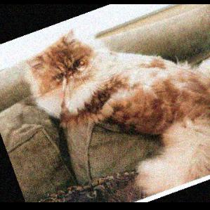
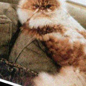
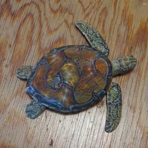
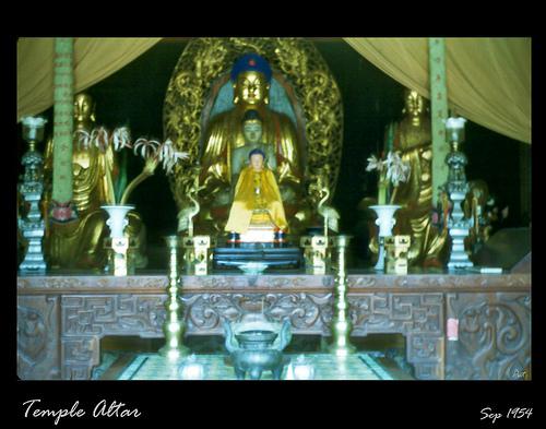
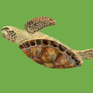
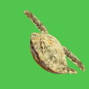
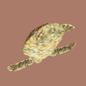
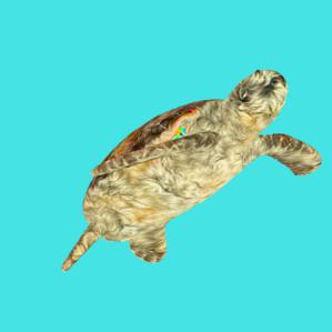
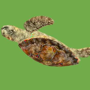
classified as turtle classified as rifle classified as other
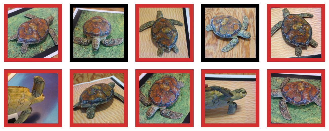
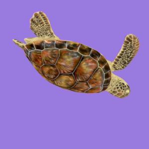
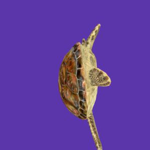
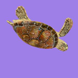
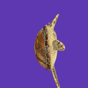
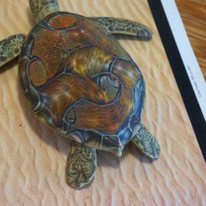
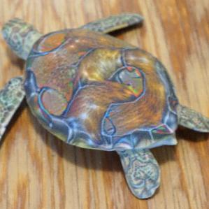
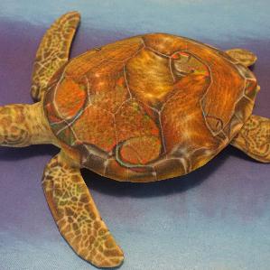
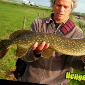
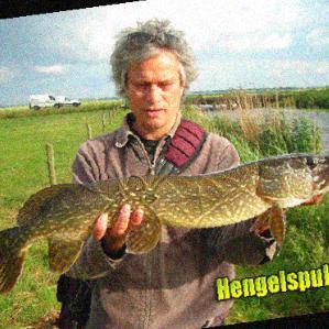
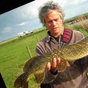
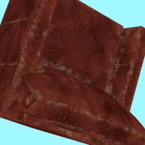
We show that neural network-based classifiers are vulnerable to physical-world adversarial examples that remain adversarial over a different viewpoints. We introduce a new algorithm for synthesizing adversarial examples that are robust over a chosen distribution of transformations, which we apply for reliably producing robust adversarial images as well as physical-world adversarial objects. Figure 2 shows an example of an adversarial object constructed using our approach, where a 3D-printed turtle is consistently classified as rifle (a target class that was selected at random) by an ImageNet classifier. In this paper, we demonstrate the efficacy and generality of our method, demonstrating conclusively that adversarial examples are a practical concern in real-world systems.
1.1 Challenges
Methods for transforming ordinary two-dimensional images into adversarial examples, including techniques such as the L-BFGS attack (Szegedy et al., 2013), FGSM (Goodfellow et al., 2015), and the CW attack (Carlini & Wagner, 2017c), are well-known. While adversarial examples generated through these techniques can transfer to the physical world (Kurakin et al., 2016), the techniques have limited success in affecting real-world systems where the input may be transformed before being fed to the classifier. Prior work has shown that adversarial examples generated using these standard techniques often lose their adversarial nature once subjected to minor transformations (Luo et al., 2016; Lu et al., 2017).
Prior techniques attempting to synthesize adversarial examples robust over any chosen distribution of transformations in the physical world have had limited success (Evtimov et al., 2017). While some progress has been made, concurrent efforts have demonstrated a small number of data points on nonstandard classifiers, and only in the two-dimensional case, with no clear generalization to three dimensions (further discussed in Section 4).
Prior work has focused on generating two-dimensional adversarial examples, even for the physical world (Sharif et al., 2016; Evtimov et al., 2017), where “viewpoints” can be approximated by an affine transformations of an original image. However, 3D objects must remain adversarial in the face of complex transformations not applicable to 2D physical-world objects, such as 3D rotation and perspective projection.
1.2 Contributions
We demonstrate the existence of robust adversarial examples and adversarial objects in the physical world. We propose a general-purpose algorithm for reliably constructing adversarial examples robust over a chosen distribution of transformations, and we demonstrate the efficacy of this algorithm in both the 2D and 3D case. We succeed in computing and fabricating physical-world 3D adversarial objects that are robust over a large, realistic distribution of 3D viewpoints, demonstrating that the algorithm successfully produces adversarial three-dimensional objects that are adversarial in the physical world. Specifically, our contributions are as follows:
-
•
We develop Expectation Over Transformation (EOT), the first algorithm that produces robust adversarial examples: single adversarial examples that are simultaneously adversarial over an entire distribution of transformations.
-
•
We consider the problem of constructing 3D adversarial examples under the EOT framework, viewing the 3D rendering process as part of the transformation, and we show that the approach successfully synthesizes adversarial objects.
-
•
We fabricate the first 3D physical-world adversarial objects and show that they fool classifiers in the physical world, demonstrating the efficacy of our approach end-to-end and showing the existence of robust physical-world adversarial objects.
2 Approach
First, we present the Expectation Over Transformation (EOT) algorithm, a general framework allowing for the construction of adversarial examples that remain adversarial over a chosen transformation distribution . We then describe our end-to-end approach for generating adversarial objects using a specialized application of EOT in conjunction with differentiating through the 3D rendering process.
2.1 Expectation Over Transformation
When constructing adversarial examples in the white-box case (that is, with access to a classifier and its gradient), we know in advance a set of possible classes and a space of valid inputs to the classifier; we have access to the function and its gradient , for any class and input . In the standard case, adversarial examples are produced by maximizing the log-likelihood of the target class over a -radius ball around the original image (which we represent as a vector of pixels each in ):
| subject to | |||||
This approach has been shown to be effective at generating adversarial examples. However, prior work has shown that these adversarial examples fail to remain adversarial under image transformations that occur in the real world, such as angle and viewpoint changes (Luo et al., 2016; Lu et al., 2017).
To address this issue, we introduce Expectation Over Transformation (EOT). The key insight behind EOT is to model such perturbations within the optimization procedure. Rather than optimizing the log-likelihood of a single example, EOT uses a chosen distribution of transformation functions taking an input controlled by the adversary to the “true” input perceived by the classifier. Furthermore, rather than simply taking the norm of to constrain the solution space, given a distance function , EOT instead aims to constrain the expected effective distance between the adversarial and original inputs, which we define as:
We use this new definition because we want to minimize the (expected) perceived distance as seen by the classifier. This is especially important in cases where has a different domain and codomain, e.g. when is a texture and is a rendering corresponding to the texture, we care to minimize the visual difference between and rather than minimizing the distance in texture space.
Thus, we have the following optimization problem:
| subject to | |||||
In practice, the distribution can model perceptual distortions such as random rotation, translation, or addition of noise. However, the method generalizes beyond simple transformations; transformations in can perform operations such as 3D rendering of a texture.
We maximize the objective via stochastic gradient descent. We approximate the gradient of the expected value through sampling transformations independently at each gradient descent step and differentiating through the transformation.
2.2 Choosing a distribution of transformations
Given its ability to synthesize robust adversarial examples, we use the EOT framework for generating 2D examples, 3D models, and ultimately physical-world adversarial objects. Within the framework, however, there is a great deal of freedom in the actual method by which examples are generated, including choice of , distance metric, and optimization method.
2.2.1 2D case
In the 2D case, we choose to approximate a realistic space of possible distortions involved in printing out an image and taking a natural picture of it. This amounts to a set of random transformations of the form , which are more thoroughly described in Section 3. These random transformations are easy to differentiate, allowing for a straightforward application of EOT.
2.2.2 3D case
We note that the domain and codomain of need not be the same. To synthesize 3D adversarial examples, we consider textures (color patterns) corresponding to some chosen 3D object (shape), and we choose a distribution of transformation functions that take a texture and render a pose of the 3D object with the texture applied. The transformation functions map a texture to a rendering of an object, simulating functions including rendering, lighting, rotation, translation, and perspective projection of the object. Finding textures that are adversarial over a realistic distribution of poses allows for transfer of adversarial examples to the physical world.
To solve this optimization problem, EOT requires the ability to differentiate though the 3D rendering function with respect to the texture. Given a particular pose and choices for all other transformation parameters, a simple 3D rendering process can be modeled as a matrix multiplication and addition: every pixel in the rendering is some linear combination of pixels in the texture (plus some constant term). Given a particular choice of parameters, the rendering of a texture can be written as for some coordinate map and background .
Standard 3D renderers, as part of the rendering pipeline, compute the texture-space coordinates corresponding to on-screen coordinates; we modify an existing renderer to return this information. Then, instead of differentiating through the renderer, we compute and then differentiate through . We must re-compute and using the renderer for each pose, because EOT samples new poses at each gradient descent step.
2.3 Optimizing the objective
Once EOT has been parameterized, i.e. once a distribution is chosen, the issue of actually optimizing the induced objective function remains. Rather than solving the constrained optimization problem given above, we use the Lagrangian-relaxed form of the problem, as Carlini & Wagner (2017c) do in the standard single-viewpoint case:
In order to encourage visual imperceptibility of the generated images, we set to be the norm in the LAB color space, a perceptually uniform color space where Euclidean distance roughly corresponds with perceptual distance (McLaren, 1976). Using distance in LAB space as a proxy for human perceptual distance is a standard technique in computer vision. Note that the can be sampled and estimated in conjunction with ; in general, the Lagrangian formulation gives EOT the ability to constrain the search space (in our case, using LAB distance) without computing a complex projection. Our optimization, then, is:
We use projected gradient descent to maximize the objective, and clip to the set of valid inputs (e.g. for images).
3 Evaluation
First, we describe our procedure for quantitatively evaluating the efficacy of EOT for generating 2D, 3D, and physical-world adversarial examples. Then, we show that we can reliably produce transformation-tolerant adversarial examples in both the 2D and 3D case. We show that we can synthesize and fabricate 3D adversarial objects, even those with complex shapes, in the physical world: these adversarial objects remain adversarial regardless of viewpoint, camera noise, and other similar real-world factors. Finally, we present a qualitative analysis of our results and discuss some challenges in applying EOT in the physical world.
3.1 Procedure
In our experiments, we use TensorFlow’s standard pre-trained InceptionV3 classifier (Szegedy et al., 2015) which has 78.0% top-1 accuracy on ImageNet. In all of our experiments, we use randomly chosen target classes, and we use EOT to synthesize adversarial examples over a chosen distribution. We measure the distance per pixel between the original and adversarial example (in LAB space), and we also measure classification accuracy (percent of randomly sampled viewpoints classified as the true class) and adversariality (percent of randomly sampled viewpoints classified as the adversarial class) for both the original and adversarial example. When working in simulation, we evaluate over a large number of transformations sampled randomly from the distribution; in the physical world, we evaluate over a large number of manually-captured images of our adversarial objects taken over different viewpoints.
Given a source object , a set of correct classes , a target class , and a robust adversarial example , we quantify the effectiveness of the adversarial example over a distribution of transformations as follows. Let be a function indicating whether the image was classified as the class :
We quantify the effectiveness of a robust adversarial example by measuring adversariality, which we define as:
This is equal to the probability that the example is classified as the target class for a transformation sampled from the distribution . We approximate the expectation by sampling a large number of values from the distribution at test time.
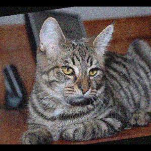
3.2 Robust 2D adversarial examples
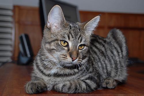
In the 2D case, we consider the distribution of transformations that includes rescaling, rotation, lightening or darkening by an additive factor, adding Gaussian noise, and translation of the image.
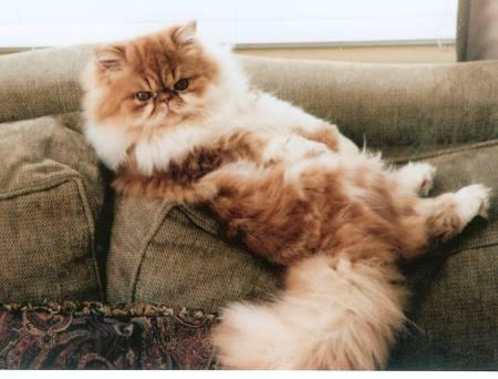
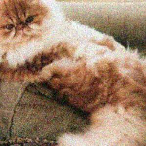
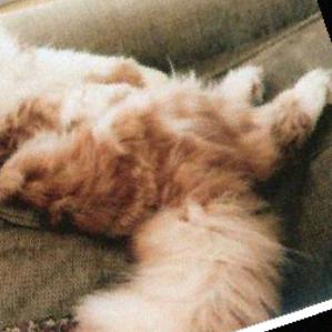
We take the first 1000 images in the ImageNet validation set, randomly choose a target class for each image, and use EOT to synthesize an adversarial example that is robust over the chosen distribution. We use a fixed in our Lagrangian to constrain visual similarity. For each adversarial example, we evaluate over 1000 random transformations sampled from the distribution at evaluation time. Table 1 summarizes the results. The adversarial examples have a mean adversariality of 96.4%, showing that our approach is highly effective in producing robust adversarial examples. Figure 2 shows one synthesized adversarial example. See the appendix for more examples.
| Images | Classification Accuracy | Adversariality | ||||||
|---|---|---|---|---|---|---|---|---|
| mean | stdev | mean | stdev | mean | ||||
| Original | 70.0% | 36.4% | 0.01% | 0.3% | 0 | |||
| Adversarial | 0.9% | 2.0% | 96.4% | 4.4% | ||||
|
|
| Original: Persian cat |
|
| 97% / 0% |

|
| 99% / 0% |
|
| 19% / 0% |

|
| 95% / 0% | |

|
|
| Adv: jacamar |

|
| 0% / 91% |
|
| 0% / 96% |

|
| 0% / 83% |
|
| 0% / 97% |
3.3 Robust 3D adversarial examples
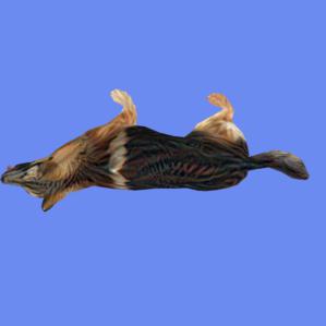
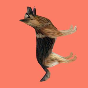
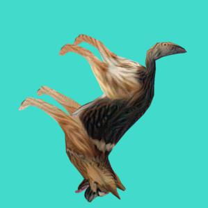
We produce 3D adversarial examples by modeling the 3D rendering as a transformation under EOT. Given a textured 3D object, we optimize the texture such that the rendering is adversarial from any viewpoint. We consider a distribution that incorporates different camera distances, lighting conditions, translation and rotation of the object, and solid background colors. We approximate the expectation over transformation by taking the mean loss over batches of size 40; furthermore, due to the computational expense of computing new poses, we reuse up to 80% of the batch at each iteration, but enforce that each batch contain at least 8 new poses. As previously mentioned, the parameters of the distribution we use is specified in the appendix, sampled as independent continuous random variables (that are uniform except for Gaussian noise). We searched over several values in our Lagrangian for each example / target class pair. In our final evaluation, we used the example with the smallest that still maintained ¿90% adversariality over 100 held out, random transformations.
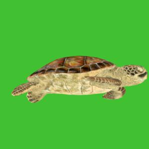
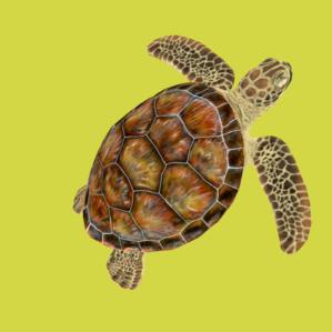
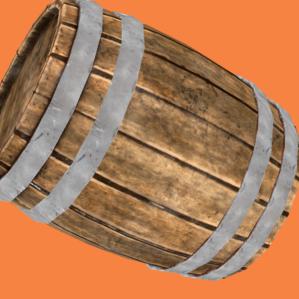
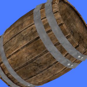
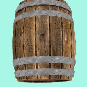
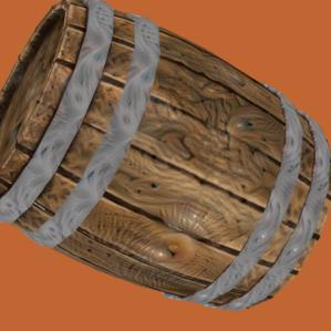
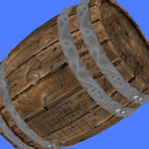
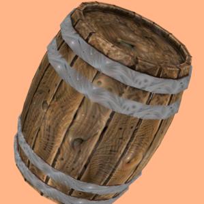
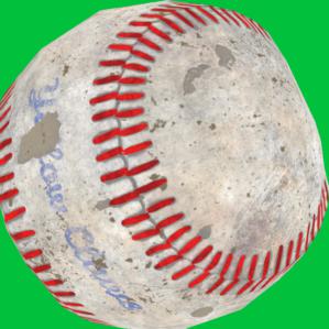
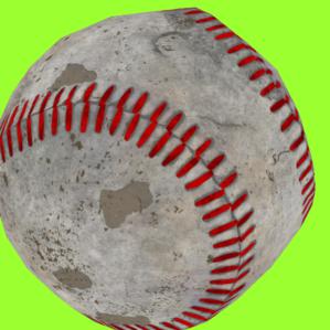
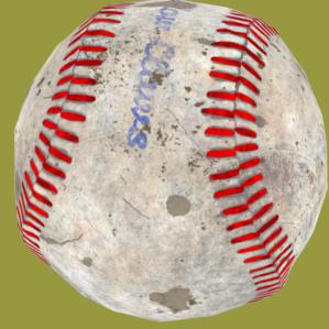
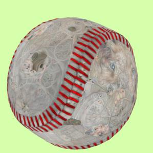
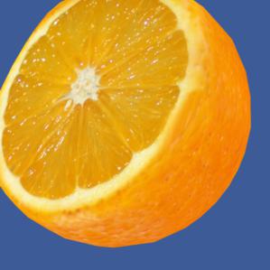
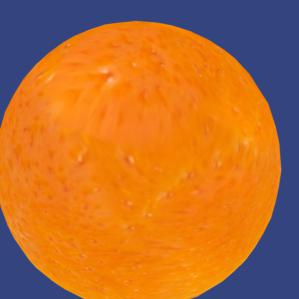
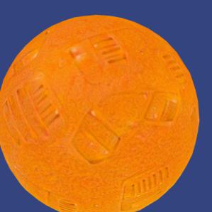
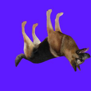
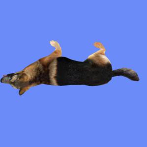
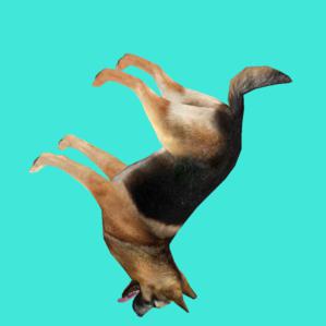
We consider 10 3D models, obtained from 3D asset sites, that represent different ImageNet classes: barrel, baseball, dog, orange, turtle, clownfish, sofa, teddy bear, car, and taxi.
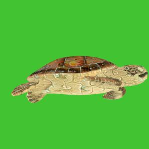
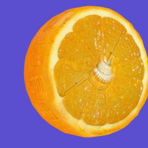
We choose 20 random target classes per 3D model, and use EOT to synthesize adversarial textures for the 3D models with minimal parameter search (four pre-chosen values were tested across each (3D model, target) pair). For each of the 200 adversarial examples, we sample 100 random transformations from the distribution at evaluation time. Table 2 summarizes results, and Figure 3 shows renderings of drawn samples, along with classification probabilities. See the appendix for more examples.
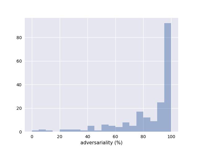
The adversarial objects have a mean adversariality of 83.4% with a long left tail, showing that EOT usually produces highly adversarial objects. See the appendix for a plot of the distribution of adversariality over the 200 examples.
| Images | Classification Accuracy | Adversariality | ||||||
|---|---|---|---|---|---|---|---|---|
| mean | stdev | mean | stdev | mean | ||||
| Original | 68.8% | 31.2% | 0.01% | 0.1% | 0 | |||
| Adversarial | 1.1% | 3.1% | 83.4% | 21.7% | ||||
| Original: turtle |
|
| 97% / 0% |
|
| 96% / 0% |
|
| 96% / 0% |
|
| 20% / 0% | |
| Adv: jigsaw puzzle |
|
| 0% / 100% |

|
| 0% / 99% |
|
| 0% / 99% |
|
| 0% / 83% |
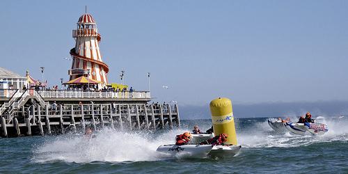
3.4 Physical adversarial examples
In the case of the physical world, we cannot capture the “true” distribution unless we perfectly model all physical phenomena. Therefore, we must approximate the distribution and perform EOT over the proxy distribution. We find that this works well in practice: we produce objects that are optimized for the proxy distribution, and we find that they generalize to the “true” physical-world distribution and remain adversarial.
Beyond modeling the 3D rendering process, we need to model physical-world phenomena such as lighting effects and camera noise. Furthermore, we need to model the 3D printing process: in our case, we use commercially available full-color 3D printing. With the 3D printing technology we use, we find that color accuracy varies between prints, so we model printing errors as well. We approximate all of these phenomena by a distribution of transformations under EOT: in addition to the transformations considered for 3D in simulation, we consider camera noise, additive and multiplicative lighting, and per-channel color inaccuracies.
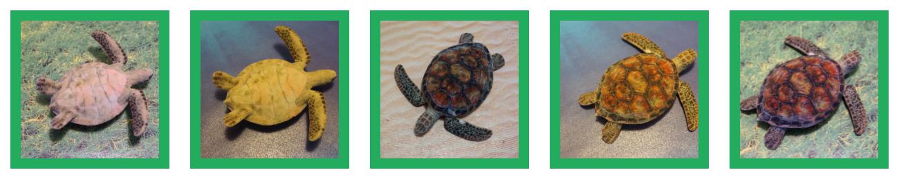
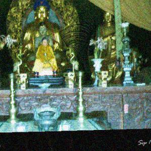
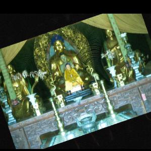
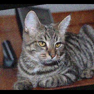
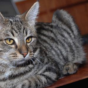
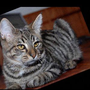
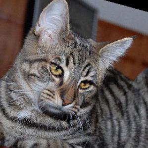
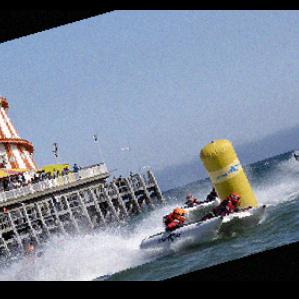
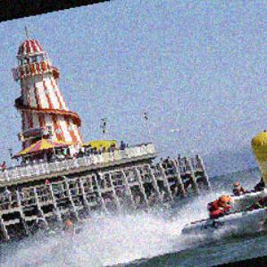
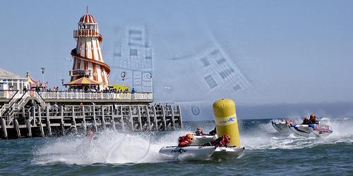
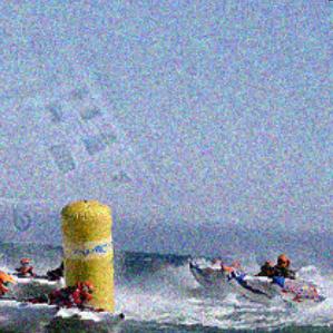
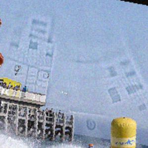
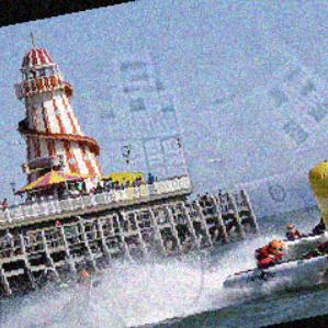
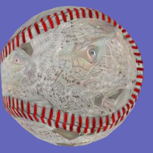
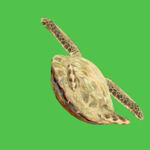
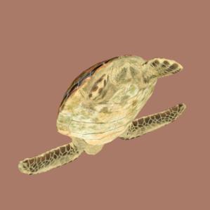
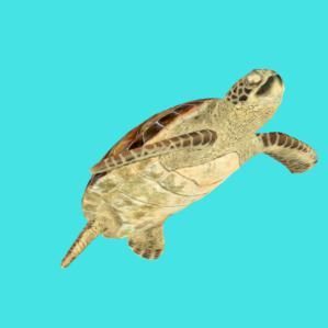
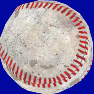
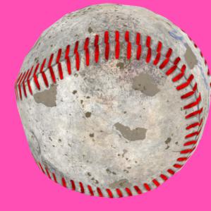
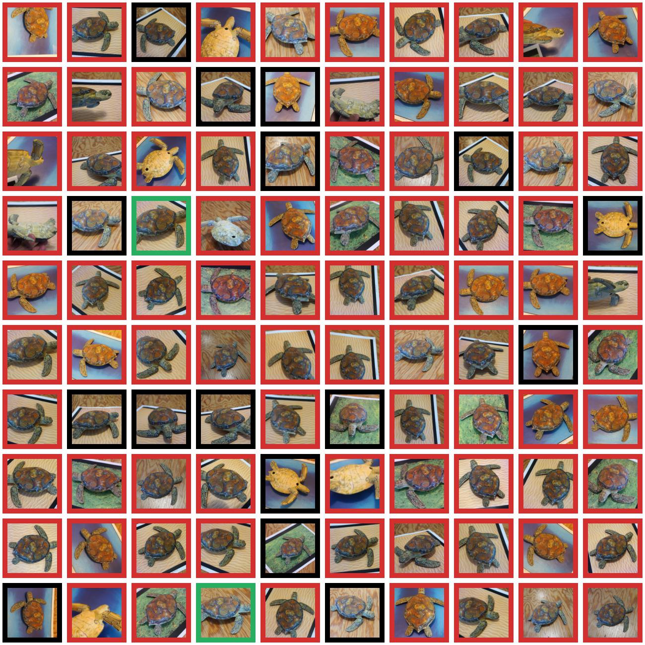
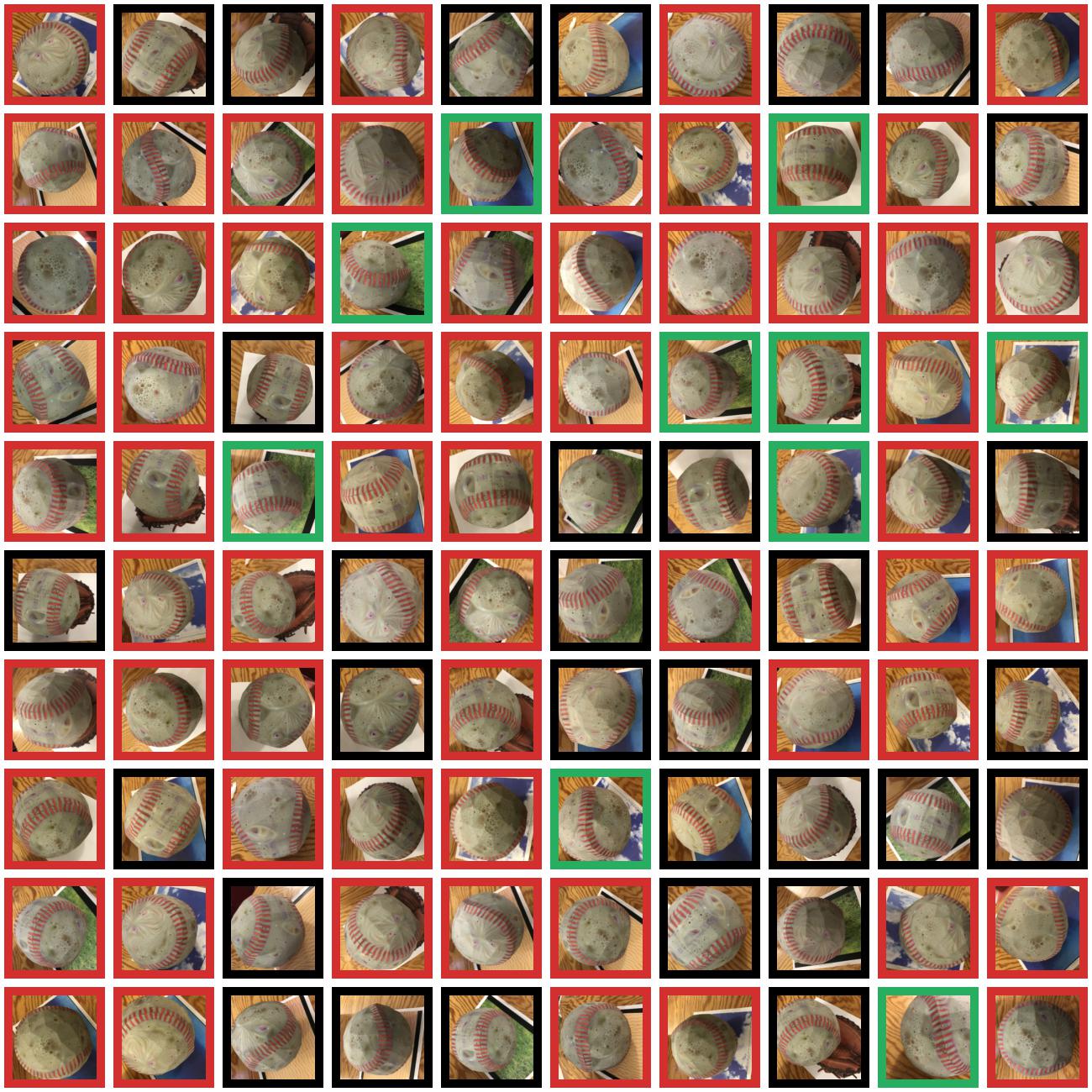
We evaluate physical adversarial examples over two 3D-printed objects: one of a turtle (where we consider any of the 5 turtle classes in ImageNet as the “true” class), and one of a baseball. The unperturbed 3D-printed objects are correctly classified as the true class with 100% accuracy over a large number of samples. Figure 4 shows example photographs of unperturbed objects, along with their classifications.
classified as turtle classified as rifle classified as other
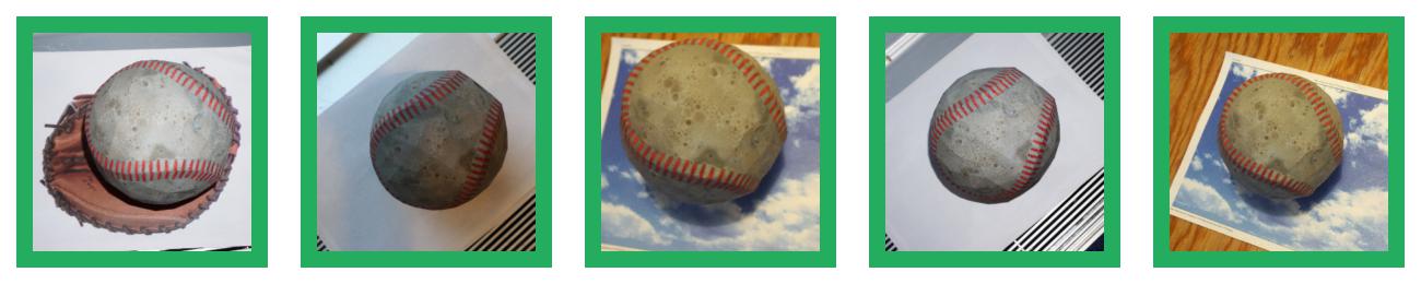
classified as baseball classified as espresso classified as other
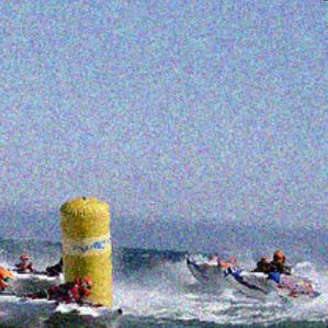
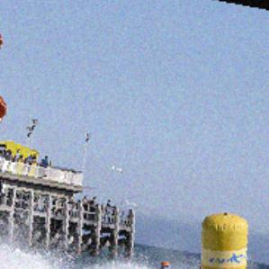
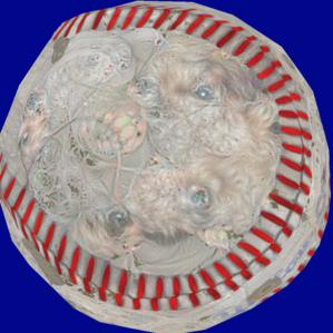
We choose target classes for each of the 3D models at random — “rifle” for the turtle, and “espresso” for the baseball — and we use EOT to synthesize adversarial examples. We evaluate the performance of our two 3D-printed adversarial objects by taking 100 photos of each object over a variety of viewpoints333Although the viewpoints were simply the result of walking around the objects, moving them up/down, etc., we do not call them “random” since they were not in fact generated numerically or sampled from a concrete distribution, in contrast with the rendered 3D examples.. Figure 5 shows a random sample of these images, along with their classifications. Table 3 gives a quantitative analysis over all images, showing that our 3D-printed adversarial objects are strongly adversarial over a wide distribution of transformations. See the appendix for more examples.
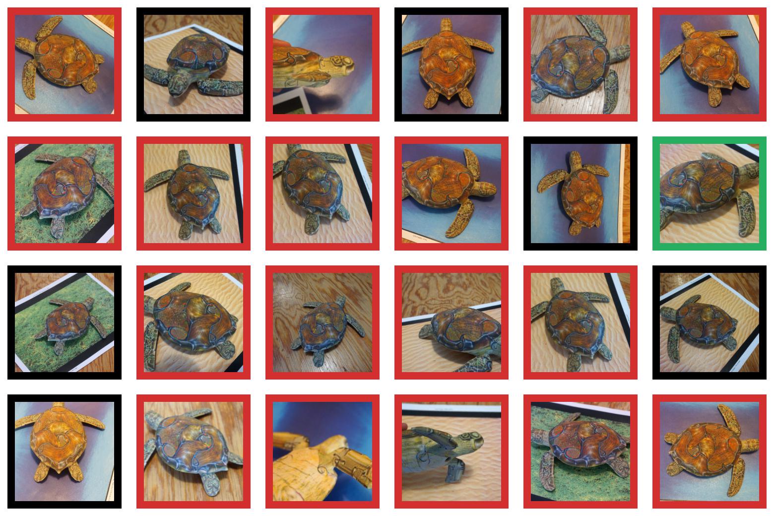
classified as turtle classified as rifle classified as other
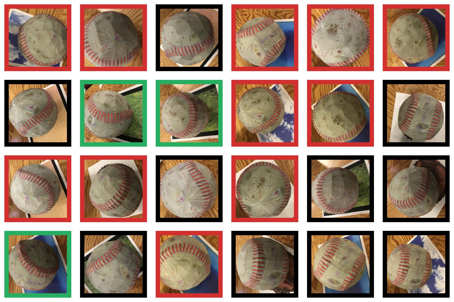
classified as baseball classified as espresso classified as other
| Object | Adversarial | Misclassified | Correct | |
|---|---|---|---|---|
| Turtle | 82% | 16% | 2% | |
| Baseball | 59% | 31% | 10% |
3.5 Discussion
Our quantitative analysis demonstrates the efficacy of EOT and confirms the existence of robust physical-world adversarial examples and objects. Now, we present a qualitative analysis of the results.
Perturbation budget.
The perturbation required to produce successful adversarial examples depends on the distribution of transformations that is chosen. Generally, the larger the distribution, the larger the perturbation required. For example, making an adversarial example robust to rotation of up to requires less perturbation than making an example robust to rotation, translation, and rescaling. Similarly, constructing robust 3D adversarial examples generally requires a larger perturbation to the underlying texture than required for constructing 2D adversarial examples.
Modeling perception.
The EOT algorithm as presented in Section 2 presents a general method to construct adversarial examples over a chosen perceptual distribution, but notably gives no guarantees for observations of the image outside of the chosen distribution. In constructing physical-world adversarial objects, we use a crude approximation of the rendering and capture process, and this succeeds in ensuring robustness in a diverse set of environments; see, for example, Figure 6, which shows the same adversarial turtle in vastly different lighting conditions. When a stronger guarantee is needed, a domain expert may opt to model the perceptual distribution more precisely in order to better constrain the search space.
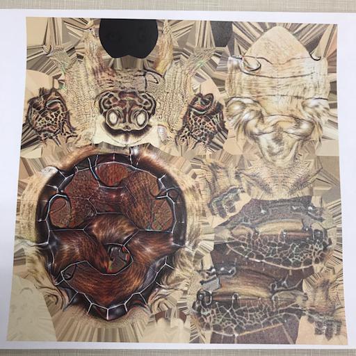
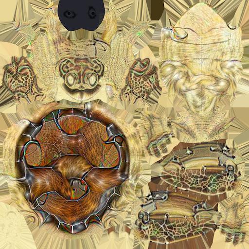
Error in printing.
We find significant error in the color accuracy of even state of the art commercially available color 3D printing; Figure 7 shows a comparison of a 3D-printed model along with a printout of the model’s texture, printed on a standard laser color printer. Still, by modeling this color error as part of the distribution of transformations in a coarse-grained manner, EOT was able to overcome the problem and produce robust physical-world adversarial objects. We predict that we could have produced adversarial examples with smaller perturbation with a higher-fidelity printing process or a more fine-grained model incorporating the printer’s color gamut.
Semantically relevant misclassification.
Interestingly, for the majority of viewpoints where the adversarial target class is not the top-1 predicted class, the classifier also fails to correctly predict the source class. Instead, we find that the classifier often classifies the object as an object that is semantically similar to the adversarial target; while generating the adversarial turtle to be classified as a rifle, for example, the second most popular class (after “rifle”) was “revolver,” followed by “holster” and then “assault rifle.” Similarly, when generating the baseball to be classified as an espresso, the example was often classified as “coffee” or “bakery.”
Breaking defenses.
The existence of robust adversarial examples implies that defenses based on randomly transforming the input are not secure: adversarial examples generated using EOT can circumvent these defenses. Athalye et al. (2018) investigates this further and circumvents several published defenses by applying Expectation over Transformation.
Limitations.
There are two possible failure cases of the EOT algorithm. As with any adversarial attack, if the attacker is constrained to too small of a ball, EOT will be unable to create an adversarial example. Another case is when the distribution of transformations the attacker chooses is too “large”. As a simple example, it is impossible to make an adversarial example robust to the function that randomly perturbs each pixel value to the interval uniformly at random.
Imperceptibility.
Note that we consider a “targeted adversarial example” to be an input that has been perturbed to misclassify as a selected class, is within the constraint bound imposed, and can be still clearly identified as the original class. While many of the generated examples are truly imperceptible from their corresponding original inputs, others exhibit noticeable perturbations. In all cases, however, the visual constraint ( metric) maintains identifiability as the original class.
4 Related Work
4.1 Adversarial examples
State of the art neural networks are vulnerable to adversarial examples (Szegedy et al., 2013; Biggio et al., 2013). Researchers have proposed a number of methods for synthesizing adversarial examples in the white-box setting (with access to the gradient of the classifier), including L-BFGS (Szegedy et al., 2013), the Fast Gradient Sign Method (FGSM) (Goodfellow et al., 2015), Jacobian-based Saliency Map Attack (JSMA) (Papernot et al., 2016b), a Lagrangian relaxation formulation (Carlini & Wagner, 2017c), and DeepFool (Moosavi-Dezfooli et al., 2015), all for what we call the single-viewpoint case where the adversary directly controls the input to the neural network. Projected Gradient Descent (PGD) can be seen as a universal first-order adversary (Madry et al., 2017). A number of approaches find adversarial examples in the black-box setting, with some relying on the transferability phenomena and making use of substitute models (Papernot et al., 2017, 2016a) and others applying black-box gradient estimation (Chen et al., 2017).
Moosavi-Dezfooli et al. (2017) show the existence of universal (image-agnostic) adversarial perturbations, small perturbation vectors that can be applied to any image to induce misclassification. Their work solves a different problem than we do: they propose an algorithm that finds perturbations that are universal over images; in our work, we give an algorithm that finds a perturbation to a single image or object that is universal over a chosen distribution of transformations. In preliminary experiments, we found that universal adversarial perturbations, like standard adversarial perturbations to single images, are not inherently robust to transformation.
4.2 Defenses
Some progress has been made in defending against adversarial examples in the white-box setting, but a complete solution has not yet been found. Many proposed defenses (Papernot et al., 2016c; Hendrik Metzen et al., 2017; Hendrycks & Gimpel, 2017; Meng & Chen, 2017; Zantedeschi et al., 2017; Buckman et al., 2018; Ma et al., 2018; Guo et al., 2018; Dhillon et al., 2018; Xie et al., 2018; Song et al., 2018; Samangouei et al., 2018) have been found to be vulnerable to iterative optimization-based attacks (Carlini & Wagner, 2016, 2017c, 2017b, 2017a; Athalye et al., 2018).
Some of these defenses that can be viewed as “input transformation” defenses are circumvented through application of EOT.
4.3 Physical-world adversarial examples
In the first work on physical-world adversarial examples, Kurakin et al. (2016) demonstrate the transferability of FGSM-generated adversarial misclassification on a printed page. In their setup, a photo is taken of a printed image with QR code guides, and the resultant image is warped, cropped, and resized to become a square of the same size as the source image before classifying it. Their results show the existence of 2D physical-world adversarial examples for approximately axis-aligned views, demonstrating that adversarial perturbations produced using FGSM can transfer to the physical world and are robust to camera noise, rescaling, and lighting effects. Kurakin et al. (2016) do not synthesize targeted physical-world adversarial examples, they do not evaluate other real-world 2D transformations such as rotation, skew, translation, or zoom, and their approach does not translate to the 3D case.
Sharif et al. (2016) develop a real-world adversarial attack on a state-of-the-art face recognition algorithm, where adversarial eyeglass frames cause targeted misclassification in portrait photos. The algorithm produces robust perturbations through optimizing over a fixed set of inputs: the attacker collects a set of images and finds a perturbation that minimizes cross entropy loss over the set. The algorithm solves a different problem than we do in our work: it produces adversarial perturbations universal over portrait photos taken head-on from a single viewpoint, while EOT produces 2D/3D adversarial examples robust over transformations. Their approach also includes a mechanism for enhancing perturbations’ printability using a color map to address the limited color gamut and color inaccuracy of the printer. Note that this differs from our approach in achieving printability: rather than creating a color map, we find an adversarial example that is robust to color inaccuracy. Our approach has the advantage of working in settings where color accuracy varies between prints, as was the case with our 3D-printer.
Concurrently to our work, Evtimov et al. (2017) proposed a method for generating robust physical-world adversarial examples in the 2D case by optimizing over a fixed set of manually-captured images. However, the approach is limited to the 2D case, with no clear translation to 3D, where there is no simple mapping between what the adversary controls (the texture) and the observed input to the classifier (an image). Furthermore, the approach requires the taking and preprocessing of a large number of photos in order to produce each adversarial example, which may be expensive or even infeasible for many objects.
Brown et al. (2016) apply our EOT algorithm to produce an “adversarial patch”, a small image patch that can be applied to any scene to cause targeted misclassification in the physical world.
Real-world adversarial examples have also been demonstrated in contexts other than image classification/detection, such as speech-to-text (Carlini et al., 2016).
5 Conclusion
Our work demonstrates the existence of robust adversarial examples, adversarial inputs that remain adversarial over a chosen distribution of transformations. By introducing EOT, a general-purpose algorithm for creating robust adversarial examples, and by modeling 3D rendering and printing within the framework of EOT, we succeed in fabricating three-dimensional adversarial objects. With access only to low-cost commercially available 3D printing technology, we successfully print physical adversarial objects that are classified as a chosen target class over a variety of angles, viewpoints, and lighting conditions by a standard ImageNet classifier. Our results suggest that adversarial examples and objects are a practical concern for real world systems, even when the examples are viewed from a variety of angles and viewpoints.
Acknowledgments
We wish to thank Ilya Sutskever for providing feedback on early parts of this work, and we wish to thank John Carrington and ZVerse for providing financial and technical support with 3D printing. We are grateful to Tatsu Hashimoto, Daniel Kang, Jacob Steinhardt, and Aditi Raghunathan for helpful comments on early drafts of this paper.
References
- Athalye et al. (2018) Athalye, A., Carlini, N., and Wagner, D. Obfuscated gradients give a false sense of security: Circumventing defenses to adversarial examples. 2018. URL https://arxiv.org/abs/1802.00420.
- Biggio et al. (2013) Biggio, B., Corona, I., Maiorca, D., Nelson, B., Šrndić, N., Laskov, P., Giacinto, G., and Roli, F. Evasion attacks against machine learning at test time. In Joint European Conference on Machine Learning and Knowledge Discovery in Databases, pp. 387–402. Springer, 2013.
- Brown et al. (2016) Brown, T. B., Mané, D., Roy, A., Abadi, M., and Gilmer, J. Defensive distillation is not robust to adversarial examples. 2016. URL https://arxiv.org/abs/1607.04311.
- Buckman et al. (2018) Buckman, J., Roy, A., Raffel, C., and Goodfellow, I. Thermometer encoding: One hot way to resist adversarial examples. International Conference on Learning Representations, 2018. URL https://openreview.net/forum?id=S18Su--CW. accepted as poster.
- Carlini & Wagner (2016) Carlini, N. and Wagner, D. Defensive distillation is not robust to adversarial examples. 2016. URL https://arxiv.org/abs/1607.04311.
- Carlini & Wagner (2017a) Carlini, N. and Wagner, D. Adversarial examples are not easily detected: Bypassing ten detection methods. AISec, 2017a.
- Carlini & Wagner (2017b) Carlini, N. and Wagner, D. Magnet and “efficient defenses against adversarial attacks” are not robust to adversarial examples. arXiv preprint arXiv:1711.08478, 2017b.
- Carlini & Wagner (2017c) Carlini, N. and Wagner, D. Towards evaluating the robustness of neural networks. In IEEE Symposium on Security & Privacy, 2017c.
- Carlini et al. (2016) Carlini, N., Mishra, P., Vaidya, T., Zhang, Y., Sherr, M., Shields, C., Wagner, D., and Zhou, W. Hidden voice commands. In 25th USENIX Security Symposium (USENIX Security 16), pp. 513–530, Austin, TX, 2016. USENIX Association. ISBN 978-1-931971-32-4. URL https://www.usenix.org/conference/usenixsecurity16/technical-sessions/presentation/carlini.
- Chen et al. (2017) Chen, P.-Y., Zhang, H., Sharma, Y., Yi, J., and Hsieh, C.-J. Zoo: Zeroth order optimization based black-box attacks to deep neural networks without training substitute models. In Proceedings of the 10th ACM Workshop on Artificial Intelligence and Security, AISec ’17, pp. 15–26, New York, NY, USA, 2017. ACM. ISBN 978-1-4503-5202-4. doi: 10.1145/3128572.3140448. URL http://doi.acm.org/10.1145/3128572.3140448.
- Dhillon et al. (2018) Dhillon, G. S., Azizzadenesheli, K., Bernstein, J. D., Kossaifi, J., Khanna, A., Lipton, Z. C., and Anandkumar, A. Stochastic activation pruning for robust adversarial defense. International Conference on Learning Representations, 2018. URL https://openreview.net/forum?id=H1uR4GZRZ. accepted as poster.
- Evtimov et al. (2017) Evtimov, I., Eykholt, K., Fernandes, E., Kohno, T., Li, B., Prakash, A., Rahmati, A., and Song, D. Robust Physical-World Attacks on Deep Learning Models. 2017. URL https://arxiv.org/abs/1707.08945.
- Goodfellow et al. (2015) Goodfellow, I. J., Shlens, J., and Szegedy, C. Explaining and harnessing adversarial examples. In Proceedings of the International Conference on Learning Representations (ICLR), 2015.
- Guo et al. (2018) Guo, C., Rana, M., Cisse, M., and van der Maaten, L. Countering adversarial images using input transformations. International Conference on Learning Representations, 2018. URL https://openreview.net/forum?id=SyJ7ClWCb. accepted as poster.
- Hendrik Metzen et al. (2017) Hendrik Metzen, J., Genewein, T., Fischer, V., and Bischoff, B. On detecting adversarial perturbations. In International Conference on Learning Representations, 2017.
- Hendrycks & Gimpel (2017) Hendrycks, D. and Gimpel, K. Early methods for detecting adversarial images. In International Conference on Learning Representations (Workshop Track), 2017.
- Kurakin et al. (2016) Kurakin, A., Goodfellow, I., and Bengio, S. Adversarial examples in the physical world. 2016. URL https://arxiv.org/abs/1607.02533.
- Lu et al. (2017) Lu, J., Sibai, H., Fabry, E., and Forsyth, D. No need to worry about adversarial examples in object detection in autonomous vehicles. 2017. URL https://arxiv.org/abs/1707.03501.
- Luo et al. (2016) Luo, Y., Boix, X., Roig, G., Poggio, T., and Zhao, Q. Foveation-based mechanisms alleviate adversarial examples. 2016. URL https://arxiv.org/abs/1511.06292.
- Ma et al. (2018) Ma, X., Li, B., Wang, Y., Erfani, S. M., Wijewickrema, S., Schoenebeck, G., Houle, M. E., Song, D., and Bailey, J. Characterizing adversarial subspaces using local intrinsic dimensionality. International Conference on Learning Representations, 2018. URL https://openreview.net/forum?id=B1gJ1L2aW. accepted as oral presentation.
- Madry et al. (2017) Madry, A., Makelov, A., Schmidt, L., Tsipras, D., and Vladu, A. Towards deep learning models resistant to adversarial attacks. 2017. URL https://arxiv.org/abs/1706.06083.
- McLaren (1976) McLaren, K. Xiii—the development of the cie 1976 (l* a* b*) uniform colour space and colour‐difference formula. Journal of the Society of Dyers and Colourists, 92(9):338–341, September 1976. doi: 10.1111/j.1478-4408.1976.tb03301.x. URL https://onlinelibrary.wiley.com/doi/abs/10.1111/j.1478-4408.1976.tb03301.x.
- Meng & Chen (2017) Meng, D. and Chen, H. MagNet: a two-pronged defense against adversarial examples. In ACM Conference on Computer and Communications Security (CCS), 2017. arXiv preprint arXiv:1705.09064.
- Moosavi-Dezfooli et al. (2015) Moosavi-Dezfooli, S., Fawzi, A., and Frossard, P. Deepfool: a simple and accurate method to fool deep neural networks. CoRR, abs/1511.04599, 2015. URL http://arxiv.org/abs/1511.04599.
- Moosavi-Dezfooli et al. (2017) Moosavi-Dezfooli, S.-M., Fawzi, A., Fawzi, O., and Frossard, P. Universal adversarial perturbations. In IEEE Conference on Computer Vision and Pattern Recognition (CVPR), 2017.
- Papernot et al. (2016a) Papernot, N., McDaniel, P., and Goodfellow, I. Transferability in machine learning: from phenomena to black-box attacks using adversarial samples. 2016a. URL https://arxiv.org/abs/1605.07277.
- Papernot et al. (2016b) Papernot, N., McDaniel, P., Jha, S., Fredrikson, M., Celik, Z. B., and Swami, A. The limitations of deep learning in adversarial settings. In IEEE European Symposium on Security & Privacy, 2016b.
- Papernot et al. (2016c) Papernot, N., McDaniel, P., Wu, X., Jha, S., and Swami, A. Distillation as a defense to adversarial perturbations against deep neural networks. In Security and Privacy (SP), 2016 IEEE Symposium on, pp. 582–597. IEEE, 2016c.
- Papernot et al. (2017) Papernot, N., McDaniel, P., Goodfellow, I., Jha, S., Celik, Z. B., and Swami, A. Practical black-box attacks against machine learning. In Proceedings of the 2017 ACM on Asia Conference on Computer and Communications Security, ASIA CCS ’17, pp. 506–519, New York, NY, USA, 2017. ACM. ISBN 978-1-4503-4944-4. doi: 10.1145/3052973.3053009. URL http://doi.acm.org/10.1145/3052973.3053009.
- Samangouei et al. (2018) Samangouei, P., Kabkab, M., and Chellappa, R. Defense-gan: Protecting classifiers against adversarial attacks using generative models. International Conference on Learning Representations, 2018. URL https://openreview.net/forum?id=BkJ3ibb0-. accepted as poster.
- Sharif et al. (2016) Sharif, M., Bhagavatula, S., Bauer, L., and Reiter, M. K. Accessorize to a crime: Real and stealthy attacks on state-of-the-art face recognition. In Proceedings of the 2016 ACM SIGSAC Conference on Computer and Communications Security, CCS ’16, pp. 1528–1540, New York, NY, USA, 2016. ACM. ISBN 978-1-4503-4139-4. doi: 10.1145/2976749.2978392. URL http://doi.acm.org/10.1145/2976749.2978392.
- Song et al. (2018) Song, Y., Kim, T., Nowozin, S., Ermon, S., and Kushman, N. Pixeldefend: Leveraging generative models to understand and defend against adversarial examples. International Conference on Learning Representations, 2018. URL https://openreview.net/forum?id=rJUYGxbCW. accepted as poster.
- Szegedy et al. (2013) Szegedy, C., Zaremba, W., Sutskever, I., Bruna, J., Erhan, D., Goodfellow, I., and Fergus, R. Intriguing properties of neural networks. 2013. URL https://arxiv.org/abs/1312.6199.
- Szegedy et al. (2015) Szegedy, C., Vanhoucke, V., Ioffe, S., Shlens, J., and Wojna, Z. Rethinking the inception architecture for computer vision. 2015. URL https://arxiv.org/abs/1512.00567.
- Xie et al. (2018) Xie, C., Wang, J., Zhang, Z., Ren, Z., and Yuille, A. Mitigating adversarial effects through randomization. International Conference on Learning Representations, 2018. URL https://openreview.net/forum?id=Sk9yuql0Z. accepted as poster.
- Zantedeschi et al. (2017) Zantedeschi, V., Nicolae, M.-I., and Rawat, A. Efficient defenses against adversarial attacks. arXiv preprint arXiv:1707.06728, 2017.
Appendix A Distributions of Transformations
Under the EOT framework, we must choose a distribution of transformations, and the optimization produces an adversarial example that is robust under the distribution of transformations. Here, we give the specific parameters we chose in the 2D (Table 4), 3D (Table 5), and physical-world case (Table 6).
Appendix B Robust 2D Adversarial Examples
Appendix C Robust 3D Adversarial Examples
Appendix D Physical Adversarial Examples
Figure 14 gives all 100 photographs of our adversarial 3D-printed turtle, and Figure 15 gives all 100 photographs of our adversarial 3D-printed baseball.
| Transformation | Minimum | Maximum |
|---|---|---|
| Scale | ||
| Rotation | ||
| Lighten / Darken | ||
| Gaussian Noise (stdev) | ||
| Translation | any in-bounds | |
| Transformation | Minimum | Maximum |
|---|---|---|
| Camera distance | ||
| X/Y translation | ||
| Rotation | any | |
| Background | (0.1, 0.1, 0.1) | (1.0, 1.0, 1.0) |
| Transformation | Minimum | Maximum |
|---|---|---|
| Camera distance | ||
| X/Y translation | ||
| Rotation | any | |
| Background | (0.1, 0.1, 0.1) | (1.0, 1.0, 1.0) |
| Lighten / Darken (additive) | ||
| Lighten / Darken (multiplicative) | ||
| Per-channel (additive) | ||
| Per-channel (multiplicative) | ||
| Gaussian Noise (stdev) | ||
|
|
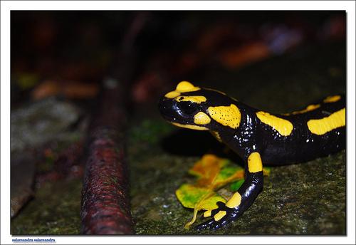
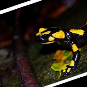
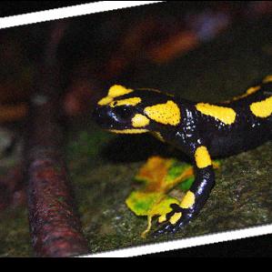
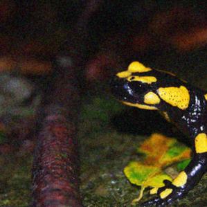
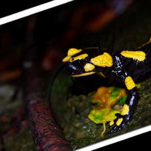
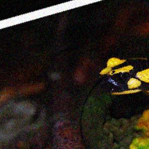
| Original: European fire salamander |
|
| : 93% | |
| : 0% |
|
| : 91% | |
| : 0% |
|
| : 93% | |
| : 0% |
|
| : 93% | |
| : 0% | |

|
|
| Adv: guacamole |
|
| : 0% | |
| : 99% |

|
| : 0% | |
| : 99% |
|
| : 0% | |
| : 96% |

|
| : 0% | |
| : 95% | |

|
|
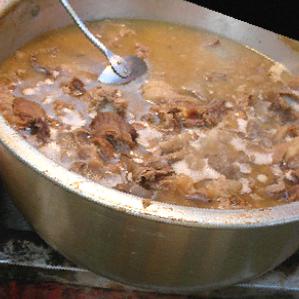
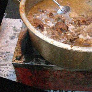
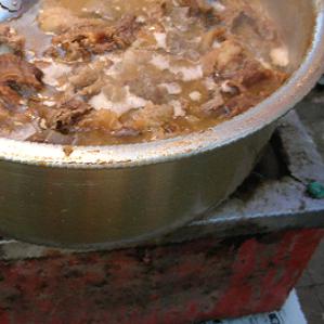
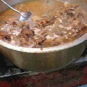
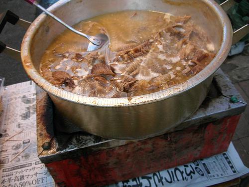
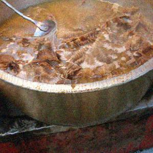
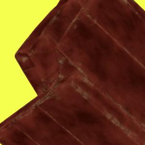
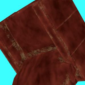
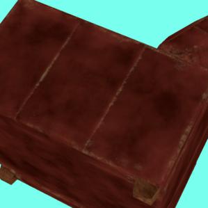
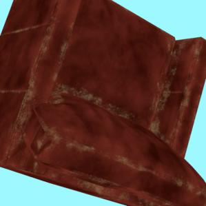
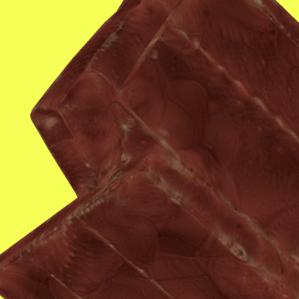
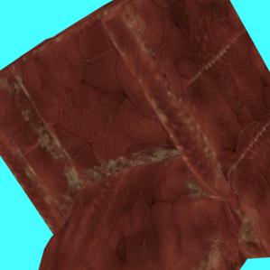
| Original: caldron |
|
| : 75% | |
| : 0% |
|
| : 83% | |
| : 0% |
|
| : 54% | |
| : 0% |
|
| : 80% | |
| : 0% | |
|
|
| Adv: velvet |

|
| : 0% | |
| : 94% |

|
| : 0% | |
| : 94% |

|
| : 1% | |
| : 91% |
|
| : 0% | |
| : 100% | |
|
|
| Original: altar |
|
| : 87% | |
| : 0% |
|
| : 38% | |
| : 0% |

|
| : 59% | |
| : 0% |

|
| : 2% | |
| : 0% | |

|
|
| Adv: African elephant |
|
| : 0% | |
| : 93% |

|
| : 0% | |
| : 87% |
|
| : 3% | |
| : 73% |
|
| : 0% | |
| : 92% |
|
|
| Original: barracouta |
|
| : 91% | |
| : 0% |

|
| : 95% | |
| : 0% |

|
| : 92% | |
| : 0% |
|
| : 92% | |
| : 0% | |

|
|
| Adv: tick |

|
| : 0% | |
| : 88% |
|
| : 0% | |
| : 99% |
|
| : 0% | |
| : 98% |

|
| : 0% | |
| : 95% | |
|
|
| Original: tiger cat |

|
| : 85% | |
| : 0% |

|
| : 91% | |
| : 0% |
|
| : 69% | |
| : 0% |
|
| : 96% | |
| : 0% | |

|
|
| Adv: tiger |
|
| : 32% | |
| : 54% |
|
| : 11% | |
| : 84% |
|
| : 59% | |
| : 22% |

|
| : 14% | |
| : 79% | |
|
|
| Original: speedboat |
|
| : 14% | |
| : 0% |
|
| : 1% | |
| : 0% |
|
| : 1% | |
| : 0% |
|
| : 1% | |
| : 0% | |
|
|
| Adv: crossword puzzle |
|
| : 3% | |
| : 91% |
|
| : 0% | |
| : 100% |

|
| : 0% | |
| : 100% |
|
| : 0% | |
| : 100% |
| Original: barrel |

|
| : 96% | |
| : 0% |
|
| : 99% | |
| : 0% |
|
| : 96% | |
| : 0% |
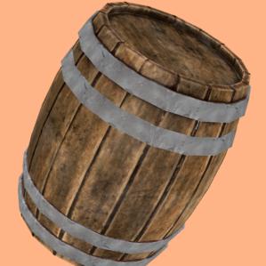
|
| : 97% | |
| : 0% | |
| Adv: guillotine |
|
| : 1% | |
| : 10% |
|
| : 0% | |
| : 95% |
|
| : 0% | |
| : 91% |
|
| : 3% | |
| : 4% | |
| Original: baseball |
|
| : 100% | |
| : 0% |
|
| : 100% | |
| : 0% |
|
| : 100% | |
| : 0% |
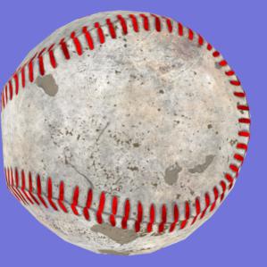
|
| : 100% | |
| : 0% | |
| Adv: green lizard |
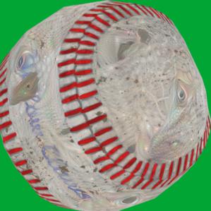
|
| : 0% | |
| : 66% |
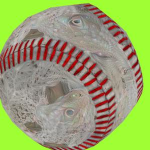
|
| : 0% | |
| : 94% |
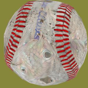
|
| : 0% | |
| : 87% |
|
| : 0% | |
| : 94% | |
| Original: turtle |
|
| : 94% | |
| : 0% |
|
| : 98% | |
| : 0% |
|
| : 90% | |
| : 0% |
|
| : 97% | |
| : 0% | |
| Adv: Bouvier des Flandres |
|
| : 1% | |
| : 1% |
|
| : 0% | |
| : 6% |
|
| : 0% | |
| : 21% |
|
| : 0% | |
| : 84% |
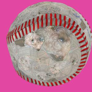
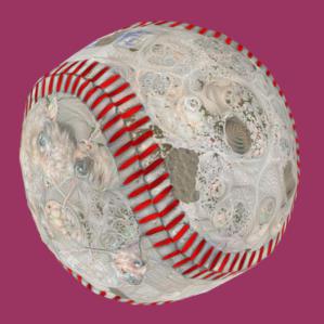
| Original: baseball |
|
| : 100% | |
| : 0% |

|
| : 100% | |
| : 0% |
|
| : 100% | |
| : 0% |

|
| : 100% | |
| : 0% | |
| Adv: Airedale |
|
| : 0% | |
| : 94% |
|
| : 0% | |
| : 6% |
|
| : 0% | |
| : 96% |
|
| : 0% | |
| : 18% | |
| Original: orange |
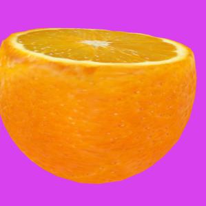
|
| : 73% | |
| : 0% |

|
| : 29% | |
| : 0% |
|
| : 20% | |
| : 0% |
|
| : 85% | |
| : 0% | |
| Adv: power drill |
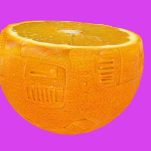
|
| : 0% | |
| : 89% |
|
| : 4% | |
| : 75% |

|
| : 0% | |
| : 98% |
|
| : 0% | |
| : 84% | |
| Original: dog |
|
| : 1% | |
| : 0% |
|
| : 32% | |
| : 0% |

|
| : 12% | |
| : 0% |
|
| : 0% | |
| : 0% | |
| Adv: bittern |

|
| : 0% | |
| : 97% |
|
| : 0% | |
| : 91% |
|
| : 0% | |
| : 98% |
|
| : 0% | |
| : 97% |
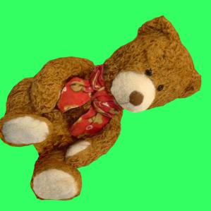
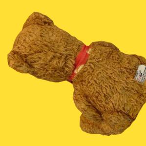
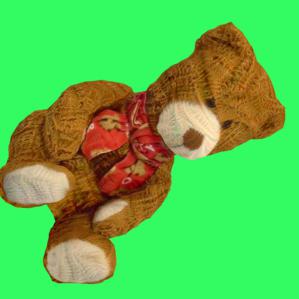
| Original: teddybear |
|
| : 90% | |
| : 0% |

|
| : 1% | |
| : 0% |

|
| : 98% | |
| : 0% |
|
| : 5% | |
| : 0% | |
| Adv: sock |
|
| : 0% | |
| : 99% |
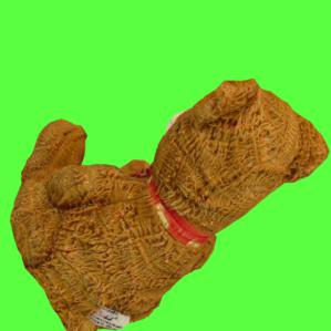
|
| : 0% | |
| : 99% |
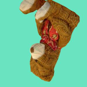
|
| : 0% | |
| : 98% |

|
| : 0% | |
| : 99% | |
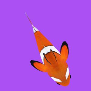
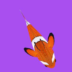
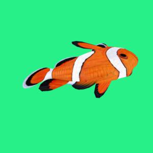
| Original: clownfish |
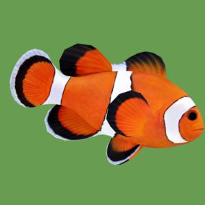
|
| : 46% | |
| : 0% |
|
| : 14% | |
| : 0% |
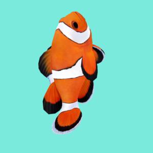
|
| : 2% | |
| : 0% |

|
| : 65% | |
| : 0% | |
| Adv: panpipe |
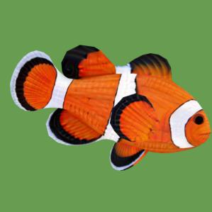
|
| : 0% | |
| : 100% |
|
| : 0% | |
| : 1% |

|
| : 0% | |
| : 12% |
|
| : 0% | |
| : 0% | |
| Original: sofa |
|
| : 15% | |
| : 0% |
|
| : 73% | |
| : 0% |
|
| : 1% | |
| : 0% |
|
| : 70% | |
| : 0% | |
| Adv: sturgeon |
|
| : 0% | |
| : 100% |
|
| : 0% | |
| : 100% |

|
| : 0% | |
| : 100% |
|
| : 0% | |
| : 100% |
classified as turtle classified as rifle classified as other
classified as baseball classified as espresso classified as other