Optically induced Lifshitz transition in bilayer graphene

Abstract

It is shown theoretically that the renormalization of the electron energy spectrum of bilayer graphene with a strong high-frequency electromagnetic field (dressing field) results in the Lifshitz transition — the abrupt change in the topology of the Fermi surface near the band edge. This effect substantially depends on the polarization of the field: The linearly polarized dressing field induces the Lifshitz transition from the quadruply-connected Fermi surface to the doubly-connected one, whereas the circularly polarized field induces the multicritical point, where the four different Fermi topologies may coexist. As a consequence, the discussed phenomenon creates physical basis to control the electronic properties of bilayer graphene with light.

I Introduction

In the last decades, the achievements in the laser technology and microwave techniques have made possible the control of various structures with a high-frequency electromagnetic field (dressing field), which is based on the Floquet theory of periodically driven quantum systems (Floquet engineering) Hanggi_98 ; Kohler_05 ; Bukov_15 ; Holthaus_16 . As a consequence, the study of condensed-matter structures strongly coupled to light has become an excited field of modern physics with the objective to find unique exploitable features. Particularly, electronic properties of various nanostructures coupled to a dressing field — including quantum wells Wagner_10 ; Teich_13 ; Kibis_14 ; Pervishko_15 ; Dini_16 ; Morina_15 , quantum rings Sigurdsson_14 ; Kibis_13 ; Koshelev_15 ; Joibari_14 , graphene Kristinsson_16 ; Kibis_16 ; Glazov_14 ; Perez_14 ; Syzranov_13 ; Kibis_11_1 ; Kibis_10 ; Oka_09 ; Kibis_17 , topological insulators Calvo_15 ; Yudin_16 ; Torres_14 ; Usaj_14 ; Ezawa_2013 , etc — are currently in the focus of attention. Developing this scientific trend in the present paper, we elaborated the theory to control the topology of the Fermi surface of bilayer graphene (BLG) with a dressing field.

BLG is the two-dimensional material consisting of two graphene monolayers, which excite enormous interest of the condensed-matter community during last years bilayer1 ; AA1 . In contrast to usual graphene monolayer with the linear (Dirac) electron dispersion CastroNeto_09 ; DasSarma_11 , the characteristic electronic properties of BLG are the massive chiral electrons and the so-called trigonal warping — the triangular perturbation of the circular iso-energetic lines near the band edge. As a consequence, the Fermi surface of BLG near the band edge consists of several electron “pockets” which are very sensitive to external impacts. Particularly, the gate voltage or uniform mechanical stress crucially changes the structure of the pockets. This results in the Lifshitz phase transition — the abrupt change in the topology of the Fermi surface Falko1 ; Falko2 ; Shtyk2017 ; Dutreix2016 . Although a strong electromagnetic field is actively studied in last years as a tool to control electronic properties of BLG — to induce the valley currents IRbil1 ; IRbil2 , to create the Floquet topological insulator IRbil3 , to produce additional Dirac points IRbil4 , etc — the optical control of the Lifshitz transition in BLG still await for consideration. The present paper is aimed to fill partially this gap in the theory.

The paper is organized as follows. In Sec. II, we apply the conventional Floquet theory to derive the effective Hamiltonian describing stationary properties of electrons in irradiated BLG. In Sec. III, we discuss the dependence of renormalized electronic characteristics of the irradiated BLG on parameters of the dressing field. The last Sec. IV contain the Conclusion and Acknowledgments.

II Model

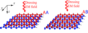
Figure 1: (Color online) Sketch of the system under consideration: AA-stacked and AB-stacked bilayer graphene subjected to an electromagnetic wave (dressing EM field) propagating perpendicularly to the graphene plane.

There are the two different crystal structures of BLG, which are known as a AA-stacked and AB-stacked BLG bilayer1 ; AA1 (see Fig. 1). Since electronic properties of BLG strongly depends on the stacking geometry, let us consider these two structures successively. For the case of the AB-stacked BLG, its low-energy electronic states are described by the four-band Hamiltonian bilayer1

$$\hat{{\cal H}}^{\prime}_{AB}=\begin{pmatrix}0&v_{1}\pi^{\dagger}&0&v_{3}\pi\\ v_{1}\pi&0&t_{1}&0\\ 0&t_{1}&0&v_{1}\pi^{\dagger}\\ v_{3}\pi^{\dagger}&0&v_{1}\pi&0\end{pmatrix},$$ (1)

where $\pi=\xi p_{x}+ip_{y}$, $p_{x,y}$ is the electron momentum in the BLG plane, $\xi=\pm 1$ is the valley index corresponding to the electron states in the two different $K$-points of the Brillouin zone, $K_{\xi}=\left({4\xi\pi}/{3a},0\right)$, $a$ is the interatomic distance, $v_{1,3}=\sqrt{3}at_{1,3}/2\hbar$ are the characteristic electron velocities, $t_{1}$ and $t_{3}$ are the characteristic energies of the interatomic electron hopping in the BLG plane and between the two graphene layers, correspondingly. Eliminating electron orbitals related to dimer sites, the Hamiltonian (1) can be reduced to the two-band effective Hamiltonian bilayer1

$$\hat{{\cal H}}_{AB}=-\alpha\begin{pmatrix}0&\left(\pi^{\dagger}\right)^{2}\\ \pi^{2}&0\end{pmatrix}+v_{3}\begin{pmatrix}0&\pi\\ \pi^{\dagger}&0\end{pmatrix},$$ (2)

where $\alpha=1/2m+v_{3}a/4\sqrt{3}\hbar$ and $m=t_{1}/2v_{1}^{2}$ is the effective electron mass. The effective Hamiltonian (2) describes the most interesting low-energy electronic properties of AB-stacked BLG — particularly, massive chiral electrons and trigonal warping bilayer1 ; BP — and, therefore, will be used by us in the following analysis. To describe the interaction between electrons in BLG and a dressing EM field within the conventional minimal coupling approach, we have to make the replacement, $\mathbf{p}\rightarrow\mathbf{p}-e\mathbf{A}$, in the Hamiltonian (2), where $\mathbf{A}=(A_{x},A_{y})$ is the vector potential of the dressing field. Assuming the EM wave to be propagating perpendicularly to the BLG plane (see Fig. 1), the vector potential can be written as

$$\mathbf{A}=\frac{E_{0}}{\omega}(\cos\theta\cos\omega t,\sin\theta\sin\omega t),$$ (3)

where $\omega$ is the frequency of the EM wave, $E_{0}$ is the amplitude of the wave, and the angle $\theta$ defines the polarization of the EM wave: The angles $\theta=0$ and $\theta=0\pi/2$ correspond the two linear polarizations, whereas the angles $\theta=\pi/4$ and $\theta=-\pi/4$ correspond to the two circular polarizations. Then the time-dependent Hamiltonian (2) can be rewritten as

$$\hat{{\cal H}}_{AB}(t)=\hat{{\cal H}}_{0}+\left[\displaystyle\sum_{n=1}^{\infty}\hat{V}_{n}e^{in\omega t}+\mathrm{H.c.}\right],$$ (4)

where the time-independent part is

$$\hat{{\cal H}}_{0}=\hat{{\cal H}}_{AB}-\frac{\alpha e^{2}E_{0}^{2}}{2\omega^{2}}\begin{pmatrix}0&\cos 2\theta\\ \cos 2\theta&0\end{pmatrix},$$ (5)

and the two first harmonics are

$$\hat{V}_{1}=\frac{\alpha|e|E_{0}\sqrt{2}}{\omega}\left[\begin{pmatrix}0&p_{x}\cos(\theta+\xi\pi/4)\\ -p_{x}\cos(\theta-\xi\pi/4)&0\end{pmatrix}\right.$$

$$+\left.\begin{pmatrix}0&ip_{y}\sin(\theta-\xi\pi/4)\\ -ip_{y}\sin(\theta+\xi\pi/4)&0\end{pmatrix}\right]$$

$$+\frac{v_{3}|e|E_{0}}{\sqrt{2}\omega}\begin{pmatrix}0&\sin(\theta+\xi\pi/4)\\ -\sin(\theta-\xi\pi/4)&0\end{pmatrix},$$ (6)

$$\hat{V}_{2}=-\frac{\alpha e^{2}E_{0}^{2}}{2\omega^{2}}\begin{pmatrix}0&\sin^{2}(\theta-\xi\pi/4)\\ \sin^{2}(\theta+\xi\pi/4)&0\end{pmatrix}.$$ (7)

Applying the standard Floquet-Magnus approach FM1 ; FM2 ; FM3 to renormalize the time-dependent Hamiltonian (4) and restricting the consideration by the terms $\sim 1/\omega^{2}$, we arrive at the effective time-independent Hamiltonian

$$\hat{{\cal H}}_{\mathrm{eff}} = \hat{{\cal H}}_{0}+\sum_{n=1}^{\infty}\frac{\left[\hat{V}_{n},\hat{V}^{\dagger}_{n}\right]}{\hbar n\omega}$$ (8)

$$+ \sum_{n=1}^{\infty}\frac{\left[\left[\hat{V}_{n},\hat{{\cal H}}_{0}\right],\hat{V}^{\dagger}_{n}\right]+\mathrm{H.c.}}{2(\hbar n\omega)^{2}}.$$

To rewrite the Hamiltonian (8) in the dimensionless form, let us introduce the dimensionless electron momentum, $\mathbf{p}\rightarrow\mathbf{p}/(v_{3}/\alpha)$, and the dimensionless electron energy, $\varepsilon\rightarrow\varepsilon/(v_{3}^{2}/\alpha)$. Then the dimensionless Hamiltonian (8) depends only on the two dimensionless parameters, $\delta_{1}={|e|E_{0}\alpha}/{v_{3}\omega}$ and $\delta_{2}={v_{3}^{2}}/{\alpha\hbar\omega}$. Physically, the first of them is the ratio of the period-averaged momentum adsorbed by an electron from the dressing field, $|e|E_{0}/\omega$, and the characteristic trigonal-warping momentum, $v_{3}/\alpha$. The second one is the ratio of the characteristic trigonal-warping energy, $v_{3}^{2}/\alpha$, and the photon energy, $\hbar\omega$. If the dressing field is high-frequency enough, the both parameters, $\delta_{1}$ and $\delta_{2}$, are small. Correspondingly, we can write the Hamiltonian as an expansion on the the small parameter, $\delta_{1}\delta_{2}\ll 1$. Then the dimensionless Hamiltonian (8) in the vicinity of the $K_{\xi}$-point ($p<1$) reads

$$\hat{{\cal H}}_{\mathrm{eff}}=\hat{{\cal H}}_{AB}+\mathbf{g}(\mathbf{p}){\bm{\sigma}},$$ (9)

where $\bm{\sigma}=(\sigma_{x},\sigma_{y},\sigma_{z})$ is the Pauli matrix vector, and $\mathbf{g}(\mathbf{p})=(g_{x},g_{y},g_{z})$ is the vector with the components

$$g_{x}={(\delta_{1}\delta_{2})^{2}}[p_{y}^{2}[\cos^{2}\theta-3-4\xi p_{x}(4\cos^{2}\theta-1)-4p^{2}\cos^{2}\theta]$$

$$+p_{x}^{2}(5-8\xi p_{x}+4p^{2})\sin^{2}\theta-\xi p_{x}\sin^{2}\theta]-\frac{\delta_{1}^{2}}{2}\cos 2\theta,$$

$$g_{y}=\frac{(\delta_{1}\delta_{2})^{2}}{2}[2p_{y}[\cos^{2}\theta+2p^{2}(3-2\cos^{2}\theta)]$$

$$+2\xi p_{x}p_{y}(2\cos^{2}\theta+6+12\xi p_{x}\cos 2\theta+4p^{2})],$$

$$g_{z}=\frac{\xi\delta_{1}^{2}\delta_{2}}{2}(1-4p^{2}){\sin 2\theta}.$$

As to the case of the AA-stacked BLG, its low-energy electronic states are described by the four-band Hamiltonian AA1

$$\hat{{\cal H}}^{\prime}_{AA}= \begin{pmatrix}0&v_{0}\pi^{\dagger}&t_{1}&0\\ v_{0}\pi&0&0&t_{1}\\ t_{1}&0&0&v_{0}\pi^{\dagger}\\ 0&t_{1}&v_{0}\pi&0\end{pmatrix},$$ (10)

where $t_{1}$ is the interlayer hopping constant and $v_{0}$ is the electron velocity in monolayer graphene. Diagonalizing the Hamiltonian (10), we arrive at the electron energy spectrum,

$$\varepsilon=\pm t_{1}\pm v_{0}p,$$ (11)

which exhibits the two monolayer graphene dispersions, $\varepsilon=\pm v_{0}p$, shifted with respect to each other by the twice interlayer hopping constant, $2t_{1}$. It should be stressed that the interlayer hopping direction of the AA-stacked BLG is orthogonal to the polarization vector of the normally incident dressing field. As a consequence, the dressing field does not affect the interlayer coupling in BLG and renormalizes electronic properties of each monolayer independently. Therefore, the effect of the dressing field on the AA-stacked BLG can be reduced to the known problem of dressed graphene monolayer Kristinsson_16 . Since the electromagnetic dressing of graphene monolayer does not lead to the Lifshitz transition, we will focus the following analysis only on the AB-stacked BLG.

III Results and Discussion

If the dressing field is linearly polarized along the $x$ axis ($\theta=0$), the Hamiltonian (9) reads

$$\hat{{\cal H}}_{\mathrm{eff}} = {\sigma}_{x}[\xi p_{x}+p_{y}^{2}[1-(\delta_{1}\delta_{2})^{2}(2+12p_{x}+4p^{2})]-{\delta_{1}^{2}}/{2}$$ (12)

$$- p_{x}^{2}]-{\sigma}_{y}[p_{y}(1-(\delta_{1}\delta_{2})^{2}[1+2p^{2}])+2\xi p_{x}p_{y}$$

$$\times (1-(\delta_{1}\delta_{2})^{2}[4+6\xi p_{x}+4p^{2}])]+O(\delta_{1}^{4}\delta_{2}^{4}).$$

Diagonalizing the Hamiltonian (12), we arrive at the energy spectrum of dressed electrons near the $K_{\pm}$ point, which is plotted in Fig. 2. In the absence of irradiation, the equi-energy map shows the four electron pockets near the $K_{\pm}$ point, which consist of one central pocket and three “leg” pockets (see Fig. 2a). These four pockets are positioned at the momenta $\mathbf{p}=0$ and $\mathbf{p}=(\xi\cos(2n\pi/3),\sin(2n\pi/3))$, where $n=0,1,2$. The dressing field distorts the pockets, shifting their position in the Brillouin zone (see Fig. 2b). Taking into account only the leading term of the Hamiltonian (12), we arrive at the equation,

$$(\delta_{1}^{2}/2+p_{x}^{2}-p_{y}^{2}-\xi p_{x})^{2}+(p_{y}+2\xi p_{x}p_{y})^{2}=0,$$

describing the centers of the shifted pockets, $p_{x}$ and $p_{y}$. This equation has the four solutions: The two ones correspond to the momenta $p_{y}=0$ and $p_{x}=(\xi\pm\sqrt{1-2\delta_{1}^{2}})/2$, whereas the other two solutions are $\mathbf{p}=(-\xi/2,\pm\sqrt{2\delta_{1}^{2}+3}/2)$. It follows from this that the first two solutions approach each other with increasing the parameter $\delta_{1}$ and merge at its critical value, $\delta^{\prime}_{1}=1/\sqrt{2}$. For $\delta_{1}>\delta^{\prime}_{1}$, the two electron pockets corresponding to these merged solutions disappear (see Fig. 2c). It should be noted that the total valley Chern number, $2\xi$, remains constant with the disappearance of the two pockets. Indeed, the central pocket of the bare bilayer graphene is characterized by the Chern number $-\xi$, whereas each of the three leg pockets has the Chern number $\xi$ (see, e.g., Ref. IRbil3, ). Under the influence of the dressing field, the central pocket “annihilates” with one of the leg pockets, which conserves the total Chern number. Since the “annihilation” of the two pockets changes the Fermi topology abruptly — from the quadruply-connected Fermi surface to the doubly-connected one — the Lifshitz transition takes place. It should be noted that it is similar to the Lifshitz transition in the strained bilayer graphene Falko1 ; Falko2 . Namely, the dressing field linearly polarized along the $x$ axis effects on BLG similarly to an uniform strain applied along the same axis. As to experimental manifestation of the Lifshitz transition in bilayer graphene, it leads to the pronounced modification of the Landau levels in the presence of a magnetic field Falko1 . If the magnetic field, $B$, is weak enough, the inverse magnetic length, $\sqrt{eB/\hbar}$, is less than the distance between the central electron pocket and the additional pockets pictured in Fig. 2 . In this case, electronic states in the different pockets are quantized by the magnetic field independently and the ground electronic state is 16-fold degenerated. As a consequence, the filling factor $\nu=16$ appears in the quantum Hall conductance. After the Lifshitz transition, only two of four electron pockets survive. This lifts the additional degeneracy and the filling factor $\nu=8$ will be observed in the Hall measurements. Thus, the Lifshitz transition leads to the possibility of optical control of quantum Hall effect, what can be observed in magnetotransport experiments.

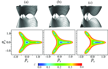
Figure 2: (Color online) The three-dimensional plots of the electron energy spectrum of irradiated AB-stacked bilayer graphene, $\varepsilon$, near the band edge (top) and the corresponding equi-energy maps (bottom) for the linearly polarized dressing field with the photon energy $\hbar\omega=25$ meV and different irradiation intensities, $I$: (a) $I=0$ kW/cm², (b) $I=10$ kW/cm², (c) $I=45$ kW/cm².

In the case of circularly polarized dressing field ($\theta=\pi/4$), the effective Hamiltonian (9) reads

$$\hat{{\cal H}}_{\mathrm{eff}}=\hat{{\cal H}}_{AB}+\frac{\xi\delta_{1}^{2}\delta_{2}}{2}(1-4p^{2})\sigma_{z}+O(\delta_{1}^{2}\delta_{2}^{2})$$ (13)

and results in the dispersion equation,

$$\varepsilon^{2}=\frac{\varepsilon_{g}^{2}}{4}+p^{2}(1-\varepsilon_{g}^{2})-2p^{3}\cos 3\phi+p^{4}(1+2\varepsilon_{g}^{2}),$$ (14)

where $\varepsilon_{g}=\sqrt{2}\delta_{1}^{2}\delta_{2}$ is the field-induced energy gap at the $K_{\pm}$ point. Opening the energy gap, the circularly polarized field effects on BLG similarly to the interlayer asymmetry induced by the gate voltage Falko2 . For the critical value of the energy gap, $\varepsilon_{g}=1$, the term $\sim p^{2}$ in Eq. (14) vanishes and the electron dispersion is $\varepsilon=\pm\sqrt{0.25-2p^{3}\cos 3\phi}$, where $\phi$ is the polar angle in the BLG plane. At the Fermi energy $\varepsilon_{F}=1/2$, this dispersion corresponds to the Fermi surface shown in Fig. 3a. The structure of the Fermi surface for different irradiation intensities, $I$, is shown in the phase diagram 3b. The critical point of the phase diagram — so-called monkey-saddle point Shtyk2017 — corresponds to the critical energy gap, $\varepsilon_{g}=1$. At this point, the Fermi surface is unstable with respect to small variations of both the Fermi energy and the irradiation intensity: It undergoes one of the four possible Lifshitz transitions depicted in Fig. 3b. Similarly to the case of linear polarization, the Lifshitz transition induced by the circularly polarized dressing field will manifest itself in magnetoconductance. Namely, the three separated pockets at the Fermi surface will lead to the filling factor $\nu=12$ in the corresponding steps of quantum Hall conductivity. Moreover, it should be noted that the critical point pictured in Fig. 3b is characterized by the diverging density of states (DoS), which is similar to the conventional Van Hove singularity. Indeed, the density of states, $\rho$, in the vicinity of the critical point reads

$$\rho(\varepsilon)=\frac{1}{(2\pi)^{2}}\int d^{2}\mathbf{p}\delta_{1}(\varepsilon-\sqrt{1/4-2p^{2}\cos 3\phi})=$$

$$=\frac{\sqrt{\varepsilon}}{9(2\pi)^{2}}\beta\left(\frac{1}{6},\frac{1}{2}\right)\left|\varepsilon^{2}-\frac{1}{4}\right|^{-1/3},$$ (15)

where $\beta(x,y)$ is the beta function (see the plot of the DoS in Fig. 3c). Since this DoS singularity leads to the instabilities of the system with respect to arbitrary weak interactions Shtyk2017 , which can be observed experimentally.

It follows from the aforesaid that a dressing field can induce the Lifshitz transitions in BLG, which depend strongly on the field polarization. Though the Hamiltonians (12) and (13) were derived within the perturbation theory, the claimed phenomenon is qualitatively the same for any strength of the electron-field coupling. It should be stressed that the exact numerical solution of the Floquet-Magnus problem (4) leads to slightly shifted critical points of the Lifshitz transitions but does not affect their structure. As to experimental observation of the optically induced Lifshitz transition, a source of intense far-infrared radiation is required. Particularly, a source of the dressing field with the photon energy 25 meV must provide the output power of several mW in order to observe the effects pictured in Fig. 3. This output power has been reported for the quantum cascade lasers (see, e.g., Ref. QCL, ) which look most appropriate for experimental observation of the discussed effects. It should be noted also that the absorption of the dressing field might provoke thermal fluctuations of electron gas. As a consequence, differentiation between different topological states can be complicated. In order to avoid this, an experimental set-up must include a high-efficient thermostat. Since the energy difference between different topological states pictured in Fig. 3 is of meV scale, the thermal fluctuations should be less than 1 K. Such a thermal stability can be provided by state-of-the-art experimental equipment. It should be noted also that the Fermi energy pictured in Fig. 3 can be modified experimentally by introducing doping on the sample. However, we have to take into account that an electromagnetic field can be considered as a dressing field within the conventional Floquet formalism if the collisional (Drude) absorption of the field by conduction electrons can be neglected (see, e.g., Refs. Kibis_14, ; Morina_15, ). To neglect the Drude absorption of a high-frequency field in a doped sample, the well-known condition, $\omega\tau\gg 1$, should be satisfied. Since the doping of the sample decreases the mean free time of conduction electron, $\tau$, the density of doping impurities should be small enough to satisfy this condition. Alternatively, the gate voltage can be used to control the Fermi energy in bilayer graphene (see, e.g., Ref. Falko2, ).

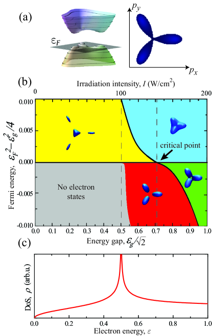
Figure 3: (Color online) The electronic structure of irradiated AB-stacked bilayer graphene for the circularly polarized dressing field with the photon energy $\hbar\omega=25$ meV: (a) Fermi surface at the monkey-saddle point; (b) Phase diagram of the Fermi surface topology; (c) Density of states spectrum near the monkey-saddle point.

IV Conclusion and acknowledgements

We demonstrated theoretically that a strong high-frequency electromagnetic field (dressing field) can be used as an effective tool to control topology of the Fermi surface of bilayer graphene (BLG). The discussed Lifshitz transition strongly depends on the polarization of the dressing field. Namely, the linearly polarized field can induce the Lifshitz transition from the quadruply-connected Fermi surface to the doubly-connected one, whereas the circularly polarized field induces the multicritical point, where the four different Fermi topologies may coexist. Physically, the linearly polarized field effects on BLG similarly to an uniform mechanical strain applied in the BLG plain along the polarization vector, whereas the circularly polarized field effects similarly to a gate voltage inducing the energy gap. Therefore, the optically induced Lifshitz transition in BLG can be used as a tool to control electronic properties of BLG-based structures.

The work was partially supported by RISE Program (project CoExAN), FP7 ITN Program (project NOTEDEV), Russian Foundation for Basic Research (project 17-02-00053), Rannis project 163082-051, and Ministry of Education and Science of Russian Federation (projects 3.4573.2017/6.7, 3.2614.2017/4.6, 3.1365.2017/4.6, 3.8884.2017/8.9 and 14.Y26.31.0015).

References

- (1) P. Hänngi, Driven quantum systems, in Quantum Transport and Dissipation edited by T. Dittrich, P. Hänggi, G.-L. Ingold, B. Kramer, G. Schön, and W. Zwerger (Wiley, Weinheim, 1998).
- (2) S. Kohler, J. Lehmann, and P. Hänngi, Driven quantum transport on the nanoscale, Phys. Rep. 406, 379–446 (2005).
- (3) M. Bukov, L. D’Alessio, and A. Polkovnikov, Universal High-Frequency Behavior of Periodically Driven Systems: from Dynamical Stabilization to Floquet Engineering, Adv. Phys. 64, 139–226 (2015).
- (4) M. Holthaus, Floquet engineering with quasienergy bands of periodically driven optical lattices, J. Phys. B 49, 013001 (2016).
- (5) M. Wagner, et al., Observation of the Intraexciton Autler-Townes Effect in GaAs/AlGaAs Semiconductor Quantum Wells, Phys. Rev. Lett. 105, 167401 (2010).
- (6) M. Teich, M. Wagner, H. Schneider, and M. Helm, Semiconductor quantum well excitons in strong, narrowband terahertz fields, New J. Phys. 15, 065007 (2013).
- (7) O. V. Kibis, How to suppress the backscattering of conduction electrons?, Europhys. Lett. 107, 57003 (2014).
- (8) S. Morina, O. V. Kibis, A. A. Pervishko, and I. A. Shelykh, Transport properties of a two-dimensional electron gas dressed by light, Phys. Rev. B 91, 155312 (2015).
- (9) A. A. Pervishko, O. V. Kibis, S. Morina, and I. A. Shelykh, Control of spin dynamics in a two-dimensional electron gas by electromagnetic dressing, Phys. Rev. B 92, 205403 (2015).
- (10) K. Dini, O. V. Kibis, and I. A. Shelykh, Magnetic properties of a two-dimensional electron gas strongly coupled to light, Phys. Rev. B 93, 235411 (2016).
- (11) O. V. Kibis, O. Kyriienko, and I. A. Shelykh, Persistent current induced by vacuum fluctuations in a quantum ring, Phys. Rev. B 87, 245437 (2013).
- (12) H. Sigurdsson, O. V. Kibis, and I. A. Shelykh, Optically induced Aharonov-Bohm effect in mesoscopic rings, Phys. Rev. B 90, 235413 (2014).
- (13) F. K. Joibari, Ya. M. Blanter, and G. E. W. Bauer, Light-induced spin polarizations in quantum rings, Phys. Rev. B 90, 155301 (2014).
- (14) K. L. Koshelev, V. Yu. Kachorovskii, and M. Titov, Resonant inverse Faraday effect in nanorings, Phys. Rev. B 92, 235426 (2015).
- (15) T. Oka and H. Aoki, Photovoltaic Hall effect in graphene, Phys. Rev. B 79, 081406 (2009).
- (16) O. V. Kibis, Metal-insulator transition in graphene induced by circularly polarized photons, Phys. Rev. B 81, 165433 (2010).
- (17) O. V. Kibis, O. Kyriienko, and I. A. Shelykh, Band gap in graphene induced by vacuum fluctuations, Phys. Rev. B 84, 195413 (2011).
- (18) S. V. Syzranov, Ya. I. Rodionov, K. I. Kugel, and F. Nori, Strongly anisotropic Dirac quasiparticles in irradiated graphene, Phys. Rev. B 88, 241112 (2013).
- (19) P. M. Perez-Piskunow, G. Usaj, C. A. Balseiro, and L. E. F. Foa Torres, Floquet chiral edge states in graphene, Phys. Rev. B 89, 121401(R) (2014).
- (20) M. M. Glazov and S. D. Ganichev, High frequency electric field induced nonlinear effects in graphene, Phys. Rep. 535, 101 (2014).
- (21) O. V. Kibis, S. Morina, K. Dini, and I. A. Shelykh, Magnetoelectronic properties of graphene dressed by a high-frequency field, Phys. Rev. B 93, 115420 (2016).
- (22) K. Kristinsson, O. V. Kibis, S. Morina, and I. A. Shelykh, Control of electronic transport in graphene by electromagnetic dressing, Sci. Rep. 6, 20082 (2016).
- (23) O. V. Kibis, K. Dini, I. V. Iorsh, and I. A. Shelykh, All-optical band engineering of gapped Dirac materials, Phys. Rev. B 95, 125401 (2017).
- (24) M. Ezawa, Photoinduced Topological Phase Transition and a Single Dirac-Cone State in Silicene, Phys. Rev. Lett. 110, 026603 (2013).
- (25) G. Usaj, P. M. Perez-Piskunow, L. E. F. Foa Torres, and C. A. Balseiro, Irradiated graphene as a tunable Floquet topological insulator, Phys. Rev. B 90, 115423 (2014).
- (26) L. E. F. Foa Torres, P. M. Perez-Piskunow, C. A. Balseiro, and G. Usaj, Multiterminal Conductance of a Floquet Topological Insulator, Phys. Rev. Lett. 113, 266801 (2014).
- (27) H. L. Calvo, L. E. F. Foa Torres, P. M. Perez-Piskunow, C. A. Balseiro, and G. Usaj, Floquet interface states in illuminated three-dimensional topological insulators, Phys. Rev. B 91, 241404(R) (2015).
- (28) D. Yudin, O. V. Kibis, and I. A. Shelykh, Optically tunable spin transport on the surface of a topological insulator, New J. Phys. 18, 103014 (2016).
- (29) E. McCann and M. Koshino, The electronic properties of bilayer graphene, Rep. Prog. Phys. 76, 056503 (2013).
- (30) C. J. Tabert, E. J. Nicol, Dynamical conductivity of AA-stacked bilayer graphene, Phys. Rev. B 86 , 075439 (2012).
- (31) A. H. Castro Neto, F. Guinea, N. M. R. Peres, K. S. Novoselov, and A. K. Geim, The electronic properties of graphene, Rev. Mod. Phys. 81, 109 (2009).
- (32) S. Das Sarma, S. Adam, E. H. Hwang, and E. Rossi, Electronic transport in two-dimensional graphene, Rev. Mod. Phys. 83, 407 (2011).
- (33) A. Varlet, D. Bischoff, P. Simonet, K. Watanabe, T. Taniguchi, T. Ihn, K. Ensslin, M. Mucha-Kruczyński, and V.I. Fal’ko, Anomalous Sequence of Quantum Hall Liquids Revealing a Tunable Lifshitz Transition in Bilayer Graphene, Phys. Rev. Lett. 113, 116602 (2014).
- (34) A. Varlet, M. Mucha-Kruczyński, D. Bischoff, P. Simonet, T. Taniguchi, K. Watanabe, V. Fal’ko, T. Ihn, and K. Ensslin, Tunable Fermi surface topology and Lifshitz transition in bilayer graphene, Synthetic Metals 210, 19-31 (2015).
- (35) A. Shtyk, G. Goldstein, and C. Chamon, Electrons at the monkey saddle: A multicritical Lifshitz point, Phys. Rev. B 95, 035137 (2017).
- (36) C. Dutreix, E. A. Stepanov, and M. I. Katsnelson, Laser-induced topological transitions in phosphorene with inversion symmetry, Phys. Rev. B 93, 241404(R) (2016).
- (37) D. S. L. Abergel and T. Chakraborty, Generation of valley polarized current in bilayer graphene, Appl. Phys. Lett. 95, 062107 (2009).
- (38) D. S. L. Abergel and T. Chakraborty, Irradiated bilayer graphene, Nanotechnology 22, 015203 (2011).
- (39) E. Suarez Morell, and L. E. F. Foa Torres, Radiation effects on the electronic properties of bilayer graphene, Phys. Rev. B 86, 125449 (2012).
- (40) W.S. Cheung and K.S. Chan, Creation of Quasi-Dirac Points in the Floquet Band Structure of Bilayer Graphene, J. Phys.: Condens. Matter 29, 215503 (2017).
- (41) G. P. Mikitik and Yu. V. Sharlai, Electron energy spectrum and the Berry phase in a graphite bilayer, Phys. Rev. B 77, 113407 (2008).
- (42) F. Casas, J. A. Oteo, and J. Ros, Floquet theory: exponential perturbative treatment, J. Phys. A 34, 3379 (2001).
- (43) N. GoldMan and J. Dalibard, Periodically Driven Quantum Systems: Effective Hamiltonians and Engineered Gauge Fields, Phys. Rev. X 4, 031027 (2014).
- (44) A. Eckardt and E. Anisimovas, High-frequency approximation for periodically driven quantum systems from a Floquet-space perspective, New J. Phys. 17, 093039 (2015).
- (45) M. I. Amanti, M. Fischer1, G. Scalari, M. Beck, and J. Faist, Low-divergence single-mode terahertz quantum cascade laser, Nat. Photonics 3, 586–590 (2009).