Semantic 3D Occupancy Mapping through Efficient High Order CRFs

Abstract

Semantic 3D mapping can be used for many applications such as robot navigation and virtual interaction. In recent years, there has been great progress in semantic segmentation and geometric 3D mapping. However, it is still challenging to combine these two tasks for accurate and large-scale semantic mapping from images. In the paper, we propose an incremental and (near) real-time semantic mapping system. A 3D scrolling occupancy grid map is built to represent the world, which is memory and computationally efficient and bounded for large scale environments. We utilize the CNN segmentation as prior prediction and further optimize 3D grid labels through a novel CRF model. Superpixels are utilized to enforce smoothness and form robust $P^{N}$ high order potential. An efficient mean field inference is developed for the graph optimization. We evaluate our system on the KITTI dataset and improve the segmentation accuracy by 10% over existing systems.

I Introduction

3D semantic mapping is important for many robot applications such as autonomous navigation and robot interaction. Robots not only need to build 3D geometric maps of the environments to avoid obstacles, but also need to recognize objects and scenes for high-level tasks. For example, autonomous vehicles need to locate and also classify vehicles and pedestrians in 3D space to keep safe. However, there are also many challenges with this task. Instead of offline batch optimization, it should be processed incrementally in real time rates and computation time should be independent of the size of environments.

The problem is composed of two parts: geometric reconstruction, and semantic segmentation. For 3D reconstruction, there has been a large amount of research on visual simultaneous localization and mapping (SLAM). The map can be composed of different geometric elements such as points [1], planes[2], and grid voxels [3] etc. For semantic segmentation, current research usually focuses on image or video segmentation for 2D pixel labeling. With the popularity of convolutional neural networks (CNN), the performance of 2D segmentation has greatly improved. However, 2D semantic reasoning is still not accurate in the case of occlusion and shadowing.

Recently, there has also been some work on semantic 3D reconstruction [4] [5]. However, most of the existing approaches suffer from a variety of limitations. For example, they cannot run incrementally in real time and cannot adapt to large scale scenarios. Some system can achieve real-time rates with GPU acceleration [5]. Different sensors can be used to accomplish the task such as RGBD cameras [6], however, they can only work indoors in small workspaces, therefore we choose stereo cameras due to their wide applicability to both indoor and outdoor environments.

In this work, we utilize CNN model to compute pixel label distributions from 2D image and transfer it to 3D grid space. We then propose a Conditional Random Field (CRF) model with higher order cliques to enforce semantic consistency among grids. The clique is generated through superpixels. We develop an efficient filter based mean field approximation inference for this hierarchical CRF. To be applicable to large-scale environments and to achieve real-time computation, a scrolling occupancy grid is built to represent the world which is memory and computationally bounded. In all, our main contributions are:

• Propose a (near) real-time incremental semantic 3D mapping system for large-scale environments using a scrolling occupancy grid

• Improve the segmentation accuracy by 10% over the state-of-the art systems on the KITTI dataset

• Develop a filter based mean filed inference for high order CRFs with robust $P^{n}$ potts model by transforming it into a hierarchical pairwise model

Figure 1: (top) Geometric and (bottom) semantic 3D reconstruction. Our system can incrementally create semantic map of large scale environments using scrolling occupancy grids in (near) real time. We utilize the latest CNN and build a novel hierarchical CRF model to optimize the label.

The paper is organized as follows. Section II presents some related work. The system contains two main parts: geometric mapping in Section III and semantic mapping in Section IV. Results and conclusions are presented in Section V and Section VI.

II Related Work

In this section, we first give an overview of the geometric 3D reconstruction and semantic reconstruction, and then introduce some work of the CRF optimization.

II-A 3D reconstruction

There are many different algorithms for geometric 3D mapping in recent years such as ORB SLAM [1], and DSO [7], which can achieve impressive results in normal environments. Their maps are usually composed of points, lines or planes. Since points are continuous in space, it is time-consuming and even intractable to perform inference each point’s label. A typical approach is to divide the space into discrete grids such as an occupancy grid [8] [9] and octomap [10], which have already been used in many dense and semantic mapping algorithms [5].

II-B Semantic reconstruction

A summary of the relevant semantic 3D mapping work is provided in Table I. A straightforward solution is to directly transfer the 2D image label to 3D by back-projection [11] without further 3D optimization. Hermans et al. [6] propose to optimize 3D label through a dense pairwise CRF. Vineet et at. [5] apply the same CRF model to large scale stereo 3D reconstruction and achieve real-time rates by GPU. Recently, more complicated high order CRF models are also used for 3D reasoning. Kundu et al. [4] model voxel’s occupancy and label in one unified CRF with high order ray factors. The super-voxels in octomap [12] or 2D superpixel [13] can also be used to form high order potential.

TABLE I: Comparison with other system

Method	Images	Incremental	High-order	Real-time
	only		CRF
Sengupta [11]	✓
Hermans [6]		✓		✓
Kundu [4]	✓	✓	✓
Sengupta [12]	✓	✓	✓
Vinnet [5]	✓	✓		✓
Zhao [13]			✓	–
Li [14]	✓	✓		✓
Ours	✓	✓	✓	✓

II-C CRF Inference

Recently, dense CRFs [15] have become a popular tool for semantic segmentation and have been applied to many systems [5] [13]. Dense CRFs can model long range relationships compared to a basic neighbour connected CRF model. More complicated CRF with high order potentials can be used to encourage label consistency within one region. Since exact inferences for CRFs is generally intractable, many approximation algorithms have been developed, such as variants of belief propagation or mean field approximation for dense CRFs [15]. Vineet et al. [16] extend this inference to CRFs with a $P^{n}$ Potts model, applied to 3D semantic mapping system[13].

III Geometric Mapping

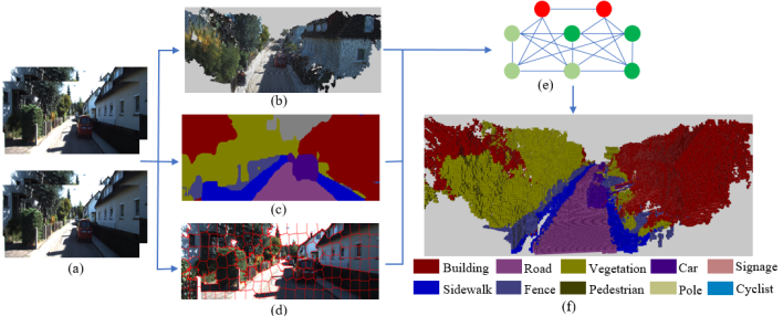
The system diagram is shown in Fig. 2. The input to our system is a series of stereo pair images and the output is an incrementally constructed 3D semantic grid map. We break the problem into two steps: geometric 3D mapping (this section) and semantic 3D labelling (next section).

Figure 2: Overview of our system. (a) Input stereo image pairs. (b) Geometric 3D reconstruction using ORB SLAM [1] and occupancy mapping [9][8]. (c) 2D semantic segmentation using CNN [17], treated as the CRF unary potential. (d) Superpixel clique generation using SLIC [18] to enforce label consistency within a region, to calculate CRF high order potential. (e) Proposed hierarchical CRF model. We develop efficient mean field inference for hierarchical CRF in 3D grid space. (f) Final semantic mapping after 3D CRF optimization.

III-A 3D mapping

We first build a 3D geometric map from stereo image pairs which contains three steps: stereo depth estimation, camera pose estimation, and 3D grid mapping.

In order to achieve a dense 3D mapping, we need to accurately estimate stereo disparity with high density. We adopt ELAS [19] which forms a triangulation on a set of support points to robustly estimate disparity in low-texture areas. We then utilize stereo ORB SLAM [1] to estimate 6DoF camera pose. It detects the ORB feature points and then minimizes the reprojection error across different views.

Since ORB SLAM only generates a sparse map of feature points which cannot be used for dense mapping, we project each frame’s estimated dense disparity to 3D space. In order to fuse the observations across different views, we change the point cloud map into 3D occupancy grids [8]. Each grid stores the probability of being occupied and is updated incrementally through ray tracing based on stereo depth measurement. To keep memory and computation efficient, the occupancy map keeps a fixed dimension and moves along with the camera. If the occupancy value exceeds a threshold, the grid will be considered as occupied and considered for the latter CRF optimization. Note that since sky has no valid depth, we ignore the classified sky pixels during occupancy mapping.

III-B Color and Label fusion

Standard occupancy grid maps only store the occupancy value, however in our case, we also need to store the color and label distribution for latter CRF optimization. Since each grid can be observed by different pixels in different frames, we need to fuse the observation before optimization. For color fusion, we directly take the mean of different color observation in different views. For the label fusion, we follow the standard Bayes’ update rule similar to that in occupancy mapping. Denote the label probability distribution of a grid at time $t$ as $x_{t}$ and the measurements till now as $z_{1:t}$. For the new combing image $z_{t}$, we first perform 2D semantic segmentation then update the 3D grid’s label based on Bayes rule:

$$\begin{split}p(x_{t}|z_{1:t})&=\frac{p(x_{t}|z_{t})p(z_{t})}{p(x_{t})}\frac{p(x_{t-1}|z_{1:t-1})}{p(z_{t}|z_{1:t-1})}\\ &\approx\frac{1}{Z}p(x_{t}|z_{t})p(x_{t-1}|z_{1:t-1})\end{split}$$ (1)

To derive the second row, we can assume the class prior $p(x_{t})$ as a constant and group $p(z_{t})/p(z_{t}|z_{1:t-1})$ as the normalization constant. So for each incoming image, the label probability fusion is simply multiplication followed by normalization. The updated $p(x_{t})$ will be further be optimized through CRF.

IV Hierarchical Semantic Mapping

After building the 3D grid map, we utilize CRFs to jointly optimize each grid’s label. We propose a general hierarchical CRF model with a robust $P^{N}$ potential and develop an efficient inference algorithm for it. Note that this CRF model can also be used for other problems such as 2D segmentation.

We start by defining each grid’s label as a random variable $x_{i}$ taking a label from a finite label set $\mathcal{L}=\{l_{1},l_{2},...,l_{k}\}$ and the joint label configuration of all $N$ grids as $\mathbf{x}\in\mathcal{L}^{N}$. Then the joint probability and Gibbs energy is defined:

$$P(\mathbf{x}|\mathbf{D})=\frac{1}{Z(\mathbf{D})}\exp(-E(\mathbf{x}|\mathbf{D}))$$ (2)

$$\begin{split}E(\mathbf{x|\mathbf{D}})=\sum_{i}\psi_{i}^{U}(x_{i})+&\sum_{i<j}\psi_{ij}^{P}(x_{i},x_{j})+\psi_{\mathbf{c}}^{HO}(\mathbf{x_{c}})\end{split}$$ (3)

where $P(\mathbf{x}|\mathbf{D})$ is the posterior probability of configuration $\mathbf{x}$ given a grid data $\mathbf{D}$, $Z(\mathbf{D})$ is the partial function for normalization. $\psi_{i}^{U}$ and $\psi_{ij}^{P}$ are the unary and pairwise potential energy. $\psi_{\mathbf{c}}^{HO}$ is the high order energy formed by all cliques $\mathbf{x_{c}}$. We will explain these three potentials in more details. Now the CRF inference problem of maximizing $P(\mathbf{x}|\mathbf{D})$ changes to find $\mathbf{x^{*}}=\arg\min_{\mathbf{x}}E(\mathbf{x}|\mathbf{D})$.

IV-A Unary potential

Unary $\psi_{i}^{U}(x_{i})$ represents the cost of a grid taking label $x_{i}$, which can also be treated as the prior distribution of variables. It is computed by the negative logarithm of the prior probability:

$$\psi_{i}^{U}(x_{i})=-\log p(x_{i})$$ (4)

where $p(x_{i})$ is the fused label distribution from Equation 2 in Section III-B. There are many approaches on 2D semantic segmentation for example TextonBoost [20] and more recent CNN [21][22]. We adopt the dilated CNN [17] simply because it directly provides the trained model. Note that it doesn’t contain post optimization such as CRF so the prediction might contain discontinuity and inconsistency between pixels as shown in Fig. 2(c).

IV-B Pairwise potential

The pairwise potential $\psi_{ij}^{P}(x_{i},x_{j})$ is adopted from [15], defined as a combination of gaussian kernels:

$$\psi_{ij}^{P}(x_{i},x_{j})=\mu(x_{i},x_{j})\sum_{m=1}^{K}w^{(m)}k^{(m)}(\textbf{f}_{i},\textbf{f}_{j})$$ (5)

where $\mu(x_{i},x_{j})$ is the label compatibility function. We use the simple Potts model $\mu(x_{i},x_{j})=[x_{i}\neq x_{j}]$, which introduces a penalty for nodes assigned different labels. Each $k^{(m)}$ is a Gaussian kernel depending on feature vectors f. We currently use two kernel potentials defined based on the color and position of 3D grid:

$$k(\textbf{f}_{i},\textbf{f}_{j}) =w_{1}\exp\Big{(}-\frac{|p_{i}-p_{j}|}{2\theta_{\alpha}^{2}}-\frac{|I_{i}-I_{j}|}{2\theta_{\beta}^{2}}\Big{)}$$ (6)

$$+w_{2}\exp\Big{(}-\frac{|p_{i}-p_{j}|}{2\theta_{\gamma}^{2}}\Big{)}$$

There are also some other features in 3D space for example surface normal [5]. However, our occupancy grid is not dense and smooth enough to compute high quality surface normals.

IV-C Hierarchical CRF Model

The above dense pairwise potential lacks the ability to express more complicated and meaningful constraints. For example in a 2D image, pixels within a homogeneous region are likely to have the same label. Thus, we design high-order potentials $\psi_{c}^{HO}(x_{c})$ to represent these constraints.

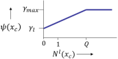
There are different models for high order potentials. The $P^{n}$ Potts model [23] rigidly enforces the nodes within a clique to take the same label which might be wrong due to inaccurate clique segmentation. Kohli et al. [24] then propose a Robust $P^{n}$ model whose cost is dependent on the number of variables taking the dominant label shown in Fig. 3. It could be treated as a soft version of $P^{n}$ Potts model. Robust $P^{n}$ is further shown to be equivalent to the minimization of a hierarchical pairwise graph with new added auxiliary variable $y_{c}$ representing the clique’s label [25] shown as the yellow nodes in Fig. 3. The robust $P^{n}$ potential for this clique is then defined as:

$$\psi^{HO}_{c}(x_{c}) =\min_{y_{c}}\psi_{c}(x_{c},y_{c})$$ (7)

$$=\min_{y_{c}}\big{(}\psi_{c}(y_{c})+\sum_{i\in c}\psi_{ci}(y_{c},x_{i})\big{)}$$

where $\psi_{c}(y_{c})$ represents the auxiliary clique variable’s unary cost. A separate classifier could be trained to compute it or we can simply use the mean of its children nodes’ unary. $\psi_{ci}(y_{c},x_{i})$ encourages the consistency between clique variable and its children nodes shown as the edge between yellow nodes and blue nodes in Fig. 3, defined as:

$$\psi_{ci}(y_{c},x_{i})=\begin{cases}0&\quad\text{if }y_{c}=x_{i}\\ k^{l}_{c}&\quad\text{Otherwise}\\ \end{cases}$$ (8)

Figure 3: (a) Robust $P^{n}$ Model cost for clique $c$ from [23]. (b) Our hierarchical CRF model by representing clique as an yellow auxiliary node. The auxiliary clique node has dense pairwise connections between each other and also has connections to its children nodes. Best viewed in color.

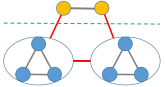
We further extend it to model the relationships between all auxiliary variables $y$ as a gaussian pairwise potential defined in Section IV-B, shown as the edges between yellow nodes. It basically encourages the label consistency between similar segment cliques. The clique variable’s feature is computed by the mean of RGB and position of all its children nodes.

In summary, let $V$ represents the set of low-level grid variables and $\mathcal{S}$ be the high-level clique variables. Then the total energy $E(\mathbf{x})$ in Equation 3 is transformed into:

$$E(\mathbf{x})= \sum_{i\in\mathcal{V}}\psi_{i}(x_{i})+\sum_{i,j\in\mathcal{V}}\psi_{ij}(x_{i},x_{j})+$$ (9)

$$\min_{\mathbf{y}}\Big{(}\sum_{c\in\mathcal{S}}\psi_{c}(x_{c},y_{c})+\sum_{c,d\in\mathcal{S}}\psi_{cd}(y_{c},y_{d})\Big{)}$$

where the first row defines the unary and pairwise potentials of low-level grid variables and the second row defines the high order potential of cliques and between cliques. Now this model is only composed of unary and pairwise terms but with more auxiliary variables.

IV-D Mean Field Inference for Hierarchical CRFs

IV-D1 Algorithm Description

Mean field inference for CRFs with $P^{n}$ potts model has been addressed by [16]. In this section, we develop efficient inference for our hierarchical CRF model with Robust $P^{n}$ model.

We approximate the target distribution $P(\mathbf{x})$ using $Q(\mathbf{x})$ with the form $Q(\mathbf{x})=\prod_{i}Q_{i}(x_{i})$, namely all variables are marginally independent. During each iteration, we first update the distribution of high-level clique variables $y_{c}$ using Equation 10 and find the MAP label assignment for them then update low-level grid nodes $x_{i}$ using Equation 11. The two mean field update rules are as follows:

$$Q^{t+1}( y_{c}=l)=\frac{1}{Z_{c}}\exp\bigg{(}-\psi_{c}(y_{c})-\sum_{d\in\mathcal{S},d\neq c}$$ (10)

$$Q_{d}(y_{d})\psi_{cd}(y_{c},y_{d})-\sum_{i\in c}Q_{i}(x_{i})\psi_{ci}(y_{c},x_{i})\bigg{)}$$

$$Q^{t+1}( x_{i}=l)=\frac{1}{Z_{i}}\exp\bigg{(}-\psi_{i}(x_{i})-\sum_{j\in\mathcal{V},j\neq i}$$ (11)

$$Q_{j}(x_{j})\psi_{ij}(x_{i},x_{j})-Q_{c}(y_{c})\psi_{ci}(y_{c},x_{i})\bigg{)}$$

IV-D2 Complexity Analysis

There are two main parts in the previous equation: dense pairwise terms $\psi_{cd}(y_{c},y_{d})$, $\psi_{ij}(x_{i},x_{j})$, and clique-children terms $\psi_{ci}(y_{c},x_{i})$.

For the dense pairwise parts, as shown by Krähenbühl [15], using the technique of Gaussian convolutions and permutohedral lattice, the time complexity of the Potts model is $\mathcal{O}(KNL)$, where $K$ is the number of kernels, $N$ is total grid number and $L$ is the labels. So in our case the computation would be $\mathcal{O}(KN_{g}L+KN_{c}L)$, where $N_{g}=|V|$, $N_{c}=|S|$ are the number of low-level grids and high-level cliques respectively.

For the clique-children terms, we need to visit each low-level grid to check its label compatibility with the clique variable. In our setting, each grid only has at most one parent clique so the computation complexity would be $\mathcal{O}(N_{g})$.

In all, the total time complexity is $\mathcal{O}(KN_{g}L+KN_{c}L+N_{g})\approx\mathcal{O}(KN_{g}L)$ as clique number $N_{c}$ is usually much smaller than grid number $N_{g}$. Therefore, it has the same algorithm complexity with dense pairwise CRF in theory, which is linear in the number of grid $N_{g}$.

V Experiments

V-A Dataset and implementation

We evaluate our system on two labelled datasets from KITTI [26]: Sengupta [11] containing 25 test images from sequence 15, and Kundu [4] containing 40 test images mainly from sequence 05. They are also used in other state-of-the-art semantic 3D mapping system [5] [12] [11]. In total, there are 11 object classes including building, road, car and so on.

As explained in Section IV-A, our unary prediction comes from the dilation CNN [17] which is trained on another sequence of KITTI dataset. Fine-tuning on the experimental dataset could also be used to further improve the accuracy. We modify the scrolling occupancy grid library [27] to maintain a 3D map. The map size is $25\times 25\times 8m^{3}$ around the camera with grid resolution $0.1m^{3}$. Larger grid volume and finer grid resolution could improve the performance but the computation time also increases quickly. Grid cells outside of the bounding area will be removed to save memory and computation for online updates, but could also be stored in memory so as to create a final complete 3D map.

We use the SLIC algorithm to generate around 150 superpixels per image, shown in Fig. 2d. We transfer the pixel-superpixel membership to 3D space by back projecting pixels to the corresponding 3D grids.

To evaluate the segmentation accuracy, we project 3D labelled grid maps onto the camera image plane, ignoring grids that are too far from the camera. We choose $40$ meters as the threshold, instead of the $25$ meters in [5]. Though further grids have larger position uncertainty and reduce the segmentation accuracy, they can improve the mapping density and can also be beneficial for other applications.

V-B Qualitative Results

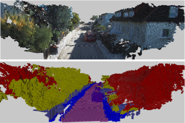
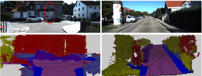
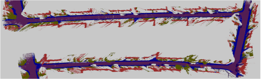
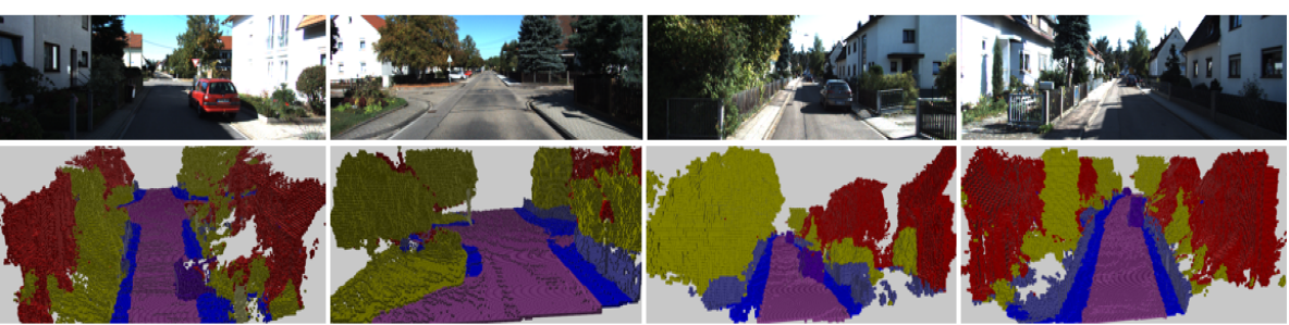
We first present some qualitative results of semantic 3D mapping in Fig. 4. Our approach can successively recognize and reconstruct classes of general objects, and even thin objects such as poles in spite of the shadows and textureless surfaces. The top view of the whole sequence (keep all grids in memory) and more examples are shown in Fig. 6.

Figure 4: Qualitative results of our 3D semantic mapping. First row: input images. Second row: semantic reconstruction scene. A thin pole is marked in red and also constructed in the map. In the second image, the building and car are clearly recognized.

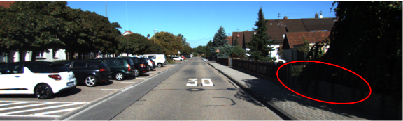
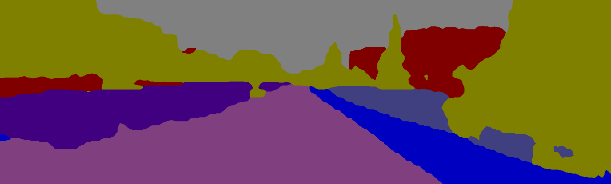
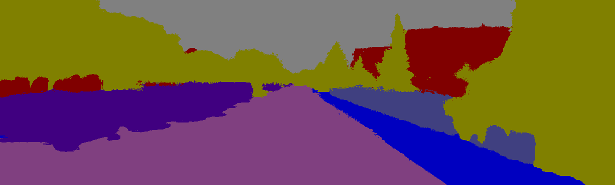
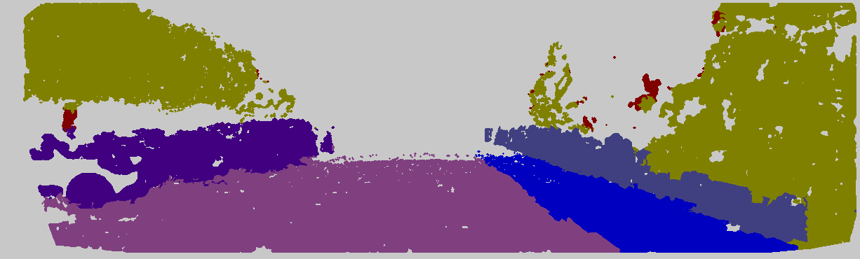
In another example of Fig. 5, we demonstrate the advantage of 3D segmentation compared to 2D. In Fig. 5, due to the dark shadow of trees, fence in the red eclipse area has similar intensity and texture with its surrounding trees thus it is very difficult to label them only from 2D image shown in Fig. 5 and Fig. 5. However, in 3D space, fence is continuous and has different shape and position compared to trees and roads thus it can be correctly labelled using 3D optimization shown in Fig. 5.

Figure 5: Examples demonstrating the advantage of 3D optimization. (a) Raw RGB image (b) 2D CNN prediction (c) 2D CRF optimization. fence on the bottom right is still wrongly labelled due to the dark shadow of trees. (d) 3D CRF optimization result (back-projection onto image plane). Gray area means no projections. Fence is now correctly labelled.

V-C Quantitative Results

In this section, we quantitatively evaluate and compare the segmentation accuracy with other approaches.

TABLE II: Comparison of 2D/3D approaches on KITTI Sengupta (seq15) dataset

Method			Building	Vegetation	Car	Road	Fence	Sidewalk	Pole	Average	Global
Accuracy	2D	Texton[20]	97.0	93.4	93.9	98.3	48.5	91.3	49.3	81.7	88.4
		CNN	98.5	97.6	96.5	98.4	77.8	87.9	51.1	86.8	94.2
	3D	Sengupta[11]	96.1	86.9	88.5	97.8	46.1	86.5	38.2	77.2	85.0
		Valentin[28]	96.4	85.4	76.8	96.9	42.7	78.5	39.3	73.7	84.5
		Sengupta[12]	89.1	81.2	72.5	97.0	45.7	73.4	3.30	66.0	78.3
		Vineet[5]	97.2	94.1	94.1	98.7	47.8	91.8	51.4	82.2	—
		Our before CRF	98.2	98.5	96.3	99.5	81.8	90.2	57.1	88.9	95.1
		Our after CRF	98.2	98.7	95.5	98.7	84.7	93.8	66.3	90.9	95.7
IoU	2D	Texton[20]	86.1	82.8	78.0	94.3	47.5	73.4	39.5	71.7
		CNN	93.3	89.8	94.1	93.4	76.4	80.0	44.1	81.7
	3D	Sengupta[11]	83.8	74.3	63.5	96.3	45.2	68.4	28.9	65.7
		Valentin[28]	82.1	73.4	67.2	91.5	40.6	62.1	25.9	63.2
		Sengupta[12]	73.8	65.2	55.8	87.8	43.7	49.1	1.9	53.9
		Vineet[5]	88.3	83.2	79.5	94.7	46.3	73.8	41.7	72.5
		Our before CRF	94.2	90.8	95.4	95.2	79.9	84.8	54.2	85.2
		Our after CRF	95.4	91.0	94.6	96.6	81.1	90.0	61.5	87.6

V-C1 Comparison with 3D system

As mentioned in Section II, different systems take different 3D geometric mapping approaches such as voxel-hashing [5], octomap [12] and our occupancy grid, therefore a common approach for comparison is to project the 3D map onto image planes. We adopt the standard metric of (class) pixel accuracy defined as TP/(TP+FP) and (class) intersection over union (IoU) defined as TP/(TP+FP+FN). T/F P/N represents true/false positive/negative.

Comparison results are shown in Table II. Global represents the overall pixel accuracy and Average represents mean class accuracy or IoU. ’—’ indicates number not provided. In total, there are 11 class in the original dataset and we select 7 common class appearing in other systems for comparison. The results of other work are taken from the paper directly. Since [12] and [28] also evaluate the signage class which is ignored here, we recompute the metric Average of their methods. Metric Global cannot be re-computed as it depends on the actual distribution but it only has about $0.1\%$ variation because signage occupies a very small area.

From the table, our method greatly outperforms other 3D systems in all categories. For the class fence, there is a significant accuracy increase of 36.3% over the state-of-the-art, and for the class pole, we achieve a 10.3% improvement. Overall, the mean class IoU is increased by 15% and global pixel accuracy is increased by 10%.

There are two main reasons why our approach outperforms existing systems. First, we use the latest the 2D CNN semantic segmentation as CRF unary shown as row ’CNN’ in the table, while existing approaches all use TextonBoost [20] shown as row ’Texton’. CNN is much more accurate than TextonBoost nearly in all categories. Even using the simple label fusion in Section III-B without further CRF optimization, the result in row Our before CRF is already more accurate than other systems. Second, we propose a new hierarchical CRF model to optimize 3D grid labels which further improves the mean IoU by 2.4% and global accuracy by 0.6%. In some class such as Sidewalk and Pole, 3D CRF optimization has about 6% improvement of IoU, which also matches the example in Fig. 5.

V-C2 Comparison of different CRF model

In this section, we compare different CRF models to demonstrate the advantage of our proposed hierarchical model. As mentioned in Section IV, our CRF model can also be applied to other optimization problems not limited to 3D mapping. So we evaluate the CRF on a 2D semantic segmentation task because it is not affected by other factors such as 3D reconstruction error, grid map resolution etc. We choose a more diverse Kundu dataset [4] for evaluation.

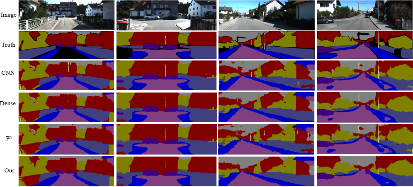
We compare with two other popular CRF models: dense CRF [15] and $P^{N}$ Potts model [16], also adopted in other 3D mapping system. All the CRF models utilize the CNN prediction as unary cost then optimize for 5 iterations. Some qualitative comparison are shown in Fig. 7 while quantitative result is shown Table III. F.W. IoU stands for frequency weighed IoU. We can see that our model has higher IoU and global accuracy. For class sign, we increase 10.5% IoU compared to other models. This is mainly because that sign is composed of triangular or square plates which usually form separate superpixels, thus suitable for our CRF model. However, some thin long objects such as Pole usually break to different superpixels, making it difficult to optimize in 2D. However, in 3D space shown in previous Table II, our CRF model can still work well because even pole is broken into multiple superpixels, its 3D position is quite different from its surroundings, therefore can still easily be classified.

TABLE III: Comparison of 2D CRF model on KITTI Kundu (seq05) dataset (IoU)

Class	CNN	Dense CRF	$P^{N}$ Potts	Our hier
Building	83.8	85.4	84.5	86.6
Sky	87.6	90.3	89.7	91.8
Road	90.0	90.2	90.0	90.1
Vegetation	83.0	83.9	82.9	83.9
Sidewalk	74.4	74.7	74.5	74.3
Car	72.5	73.8	73.0	73.1
Sign	23.1	29.3	24.7	40.6
Fence	69.5	70.4	69.5	70.1
Pole	33.6	30.6	32.4	23.5
Mean IoU	68.6	69.6	69.0	70.3
F.W IoU	81.5	82.6	81.9	82.7
Global Acc	89.9	90.5	90.1	90.6

V-D Time analysis

We also provide time analysis of different components in our system. Except for the CNN unary prediction, all other computation are implemented on desktop CPU Intel i7-4790. CNN prediction time is not included here as it depends on the model complexity and GPU power. In fact, there are also some fast and lightweight CNNs that could even run in real time on embedded system [29].

There are five main components of our system shown in Table IV. The first three parts utilize the existing public libraries and can further be computed in parallel threads to improve speed. From the label fusion in Section III-B, the grid probability distribution from previous frames is updated and further optimized by the current frame’s observation. Since each frame only updates a small part of the 3D grid map, we only need to optimize for a few iterations until convergence. Through our test, even one single mean-field update is enough to produce good results. In Table II, the result is also reported where CRF iteration is set to one.

From the table, in the current settings, the grid optimization can run at 2Hz for hierarchical CRF or 2.5Hz without high order CRF potential, slower compared to the image frame rates (10Hz). As analyzed in Section IV-D2, the computation $\mathcal{O}(KNL)$ is linear in the number of grids and label. There are several possible ways to improve the speed. Firstly, we can reduce the grid size or grid resolution to reduce the number of variables $N$ in the CRF optimization. However, this might increase the 3D reconstruction error and may not qualify for other needs. Secondly, reduce the number of labels $L$. If we only optimize for 7 main classes instead of current 11 classes, the speed can be almost doubled. Thirdly, GPU could also be used for parallel mean field updates which has been used in [5]. Lastly, we actually don’t need to process each frame as adjacent frames may appear quite similar and have small affect the 3D map. Through our test, by processing every four frames to satisfy real-time rates, the global accuracy only reduces from $95.7$ to $95.3$ and IoU reduces from $87.6$ to $86.3$.

TABLE IV: Time analysis of our algorithm.

Method	Time(s)
Dense Disparity	0.416
State Estimation	0.102
Superpixel Generation	0.115
Occupancy Mapping	0.295
CRF w/o Hierarchical	0.53/0.38

Figure 6: Visualization of 3D semantic mapping. (a) top view of 3D mapping over long sequence (850 images) of KITTI sequence 5. It demonstrates that our algorithm work well in large scale environments. (b) More 3D reconstruction examples with different scenarios.

Figure 7: Comparison of different CRF model on 2D semantic segmentation task in KITTI sequence 5. Dense stands for dense CRF. $P^{N}$ stands for high order CRF with $P^{N}$ Potts model. The last line is our proposed hierarchical CRF with robust $P^{N}$ model. The black area in truth image is not labelled. Our method on the bottom row has better overall performance for example the sky region in the third image and road on the last image.

VI Conclusion and Future Work

In this paper, we presented a 3D online semantic mapping system using stereo cameras in (near) real time. Scrolling occupancy grid maps are used to represent the world and are able to adapt to large-scale environments with bounded computation and memory. We first utilize the latest 2D CNN segmentation as prior prediction then further optimize grid labels through a hierarchical CRF model. Superpixels are utilized to enforce smoothness. Efficient mean field inference for the high order CRF with robust $P^{N}$ potential is achieved by transforming it into a hierarchical pairwise CRF. Experiments on the KITTI dataset demonstrate that our approach outperforms the state-of-the-art approaches in terms of segmentation accuracy by 10%.

Our algorithm can be used by many applications such as virtual interactions and robot navigation. In the future, we are interested in creating more abstract and high level representation of the environments such as planes and objects. Faster implementation on GPU could also be explored.

References

- [1] Raul Mur-Artal, JMM Montiel, and Juan D Tardos. ORB-SLAM: a versatile and accurate monocular SLAM system. Robotics, IEEE Transactions on, 31(5):1147–1163, 2015.
- [2] Shichao Yang, Yu Song, Michael Kaess, and Sebastian Scherer. Pop-up SLAM: a semantic monocular plane slam for low-texture environments. In Intelligent Robots and Systems (IROS), 2016 IEEE international conference on. IEEE, 2016.
- [3] Richard A Newcombe, Shahram Izadi, Otmar Hilliges, David Molyneaux, David Kim, Andrew J Davison, Pushmeet Kohi, Jamie Shotton, Steve Hodges, and Andrew Fitzgibbon. Kinectfusion: Real-time dense surface mapping and tracking. In Mixed and augmented reality (ISMAR), 2011 10th IEEE international symposium on, pages 127–136. IEEE, 2011.
- [4] Abhijit Kundu, Yin Li, Frank Dellaert, Fuxin Li, and James M Rehg. Joint semantic segmentation and 3d reconstruction from monocular video. In European Conference on Computer Vision, pages 703–718. Springer, 2014.
- [5] Vibhav Vineet, Ondrej Miksik, Morten Lidegaard, Matthias Nießner, Stuart Golodetz, Victor A Prisacariu, Olaf Kähler, David W Murray, Shahram Izadi, Patrick Pérez, et al. Incremental dense semantic stereo fusion for large-scale semantic scene reconstruction. In 2015 IEEE International Conference on Robotics and Automation (ICRA), pages 75–82. IEEE, 2015.
- [6] Alexander Hermans, Georgios Floros, and Bastian Leibe. Dense 3d semantic mapping of indoor scenes from rgb-d images. In 2014 IEEE International Conference on Robotics and Automation (ICRA), pages 2631–2638. IEEE, 2014.
- [7] Jakob Engel, Vladlen Koltun, and Daniel Cremers. Direct sparse odometry. arXiv preprint arXiv:1607.02565, 2016.
- [8] Zheng Fang, Shichao Yang, Sezal Jain, Geetesh Dubey, Stephan Roth, Silvio Maeta, Stephen Nuske, Yu Zhang, and Sebastian Scherer. Robust autonomous flight in constrained and visually degraded shipboard environments. Journal of Field Robotics, 2016.
- [9] Sebastian Scherer, Joern Rehder, Supreeth Achar, Hugh Cover, Andrew Chambers, Stephen Nuske, and Sanjiv Singh. River mapping from a flying robot: state estimation, river detection, and obstacle mapping. Autonomous Robots, 33(1-2):189–214, 2012.
- [10] Armin Hornung, Kai M Wurm, Maren Bennewitz, Cyrill Stachniss, and Wolfram Burgard. Octomap: An efficient probabilistic 3d mapping framework based on octrees. Autonomous Robots, 34(3):189–206, 2013.
- [11] Sunando Sengupta, Eric Greveson, Ali Shahrokni, and Philip HS Torr. Urban 3d semantic modelling using stereo vision. In Robotics and Automation (ICRA), 2013 IEEE International Conference on, pages 580–585. IEEE, 2013.
- [12] Sunando Sengupta and Paul Sturgess. Semantic octree: Unifying recognition, reconstruction and representation via an octree constrained higher order mrf. In 2015 IEEE International Conference on Robotics and Automation (ICRA), pages 1874–1879. IEEE, 2015.
- [13] Zhe Zhao and Xiaoping Chen. Building 3d semantic maps for mobile robots using rgb-d camera. Intelligent Service Robotics, 9(4):297–309, 2016.
- [14] Xuanpeng Li and Rachid Belaroussi. Semi-dense 3d semantic mapping from monocular slam. arXiv preprint arXiv:1611.04144, 2016.
- [15] Philipp Krähenbühl and Vladlen Koltun. Efficient inference in fully connected crfs with gaussian edge potentials. Advances in Neural Information Processing Systems (NIPS), 2011.
- [16] Vibhav Vineet, Jonathan Warrell, and Philip HS Torr. Filter-based mean-field inference for random fields with higher-order terms and product label-spaces. International Journal of Computer Vision, 110(3):290–307, 2014.
- [17] Fisher Yu and Vladlen Koltun. Multi-scale context aggregation by dilated convolutions. International Conference on Learning Representations (ICLR), 2016.
- [18] Radhakrishna Achanta, Appu Shaji, Kevin Smith, Aurelien Lucchi, Pascal Fua, and Sabine Susstrunk. Slic superpixels compared to state-of-the-art superpixel methods. Pattern Analysis and Machine Intelligence, IEEE Transactions on, 34(11):2274–2282, 2012.
- [19] Andreas Geiger, Martin Roser, and Raquel Urtasun. Efficient large-scale stereo matching. In Asian conference on computer vision, pages 25–38. Springer, 2010.
- [20] Jamie Shotton, Matthew Johnson, and Roberto Cipolla. Semantic texton forests for image categorization and segmentation. In Computer vision and pattern recognition, 2008. CVPR 2008. IEEE Conference on, pages 1–8. IEEE, 2008.
- [21] Jonathan Long, Evan Shelhamer, and Trevor Darrell. Fully convolutional networks for semantic segmentation. In Proceedings of the IEEE Conference on Computer Vision and Pattern Recognition, pages 3431–3440, 2015.
- [22] Shichao Yang, Daniel Maturana, and Sebastian Scherer. Real-time 3D scene layout from a single image using convolutional neural networks. In Robotics and automation (ICRA), IEEE international conference on, pages 2183 – 2189. IEEE, 2016.
- [23] Pushmeet Kohli, M Pawan Kumar, and Philip HS Torr. P3 & beyond: Solving energies with higher order cliques. In 2007 IEEE Conference on Computer Vision and Pattern Recognition, pages 1–8. IEEE, 2007.
- [24] Pushmeet Kohli, Philip HS Torr, et al. Robust higher order potentials for enforcing label consistency. International Journal of Computer Vision, 82(3):302–324, 2009.
- [25] Chris Russell, Pushmeet Kohli, Philip HS Torr, et al. Associative hierarchical crfs for object class image segmentation. In Computer Vision, 2009 IEEE 12th International Conference on, pages 739–746. IEEE, 2009.
- [26] Andreas Geiger, Philip Lenz, and Raquel Urtasun. Are we ready for autonomous driving? the kitti vision benchmark suite. In Computer Vision and Pattern Recognition (CVPR), 2012 IEEE Conference on, pages 3354–3361. IEEE, 2012.
- [27] Daniel Maturana. Scrollgrid, http://dx.doi.org/10.5281/zenodo.832977, August 2016.
- [28] Julien PC Valentin, Sunando Sengupta, Jonathan Warrell, Ali Shahrokni, and Philip HS Torr. Mesh based semantic modelling for indoor and outdoor scenes. In Proceedings of the IEEE Conference on Computer Vision and Pattern Recognition, pages 2067–2074, 2013.
- [29] Adam Paszke, Abhishek Chaurasia, Sangpil Kim, and Eugenio Culurciello. Enet: A deep neural network architecture for real-time semantic segmentation. arXiv preprint arXiv:1606.02147, 2016.