A locking-free optimal control problem with $L^{1}$ cost for optimal placement of control devices in Timoshenko beam

Abstract.

The numerical approximation of an optimal control problem with $L^{1}$-control of a Timoshenko beam is considered and analyzed by using the finite element method. From the practical point of view, inclusion of the $L^{1}$–norm in the cost functional is interesting in the case of beam vibration model, since the sparsity enforced by the $L^{1}$–norm is very useful for localizing actuators or control devices. The discretization of the control variables is performed by using piecewise constant functions. The states and the adjoint states are approximated by a locking free scheme of linear finite elements. Analogously to the purely $L^{2}$–norm penalized optimal control, it is proved that this approximation have optimal convergence order, which do not depend on the thickness of the beam.

1. Introduction

The optimal control and stability properties of flexible beams have been considered by many researchers in the last years, mainly motivated for science and engineering applications (see, for instance, [8]). A relevant fact in this area is to develop efficient numerical methods for both: the control problem and the beam structure model (seen as state equation), respectively.

The numerical analysis of optimal control problems has been an active research area, in particular in the derivation of a priori error estimates arising in its numerical approximation. Also, the analysis of problems involving a functional that contains an $L^{1}(\Omega)$–control cost term has been considered in the literature. In [2] we can find a review on sparse control for differential equations. The article [15] seems to be the first to provide an analysis when the distributed control problem associated to a linear elliptic equation is considered. The author utilizes a regularization technique that involves an $L^{2}(\Omega)$–control cost term and analyze optimality conditions and study the convergence properties of a semismooth Newton method for computing numerically the optimal control. These results were later extended in [16], where the authors obtain rates of convergence with respect to a regularization parameter. Subsequently, in [3], the authors consider a semilinear and elliptic PDE as state equation and analyze second order optimality conditions. Simultaneously, the numerical analysis based on finite element discretizationis considered in [16], where the state equation is a linear and elliptic PDE and in [4, 3] where an extensions to the semilinear case is introduced. This kind of problem are also extended by considering the parabolic case in [5] and fractional diffusion state equation in [14].

On the other hand, the most common mathematical model used for thick beam is the Timoshenko model. In [12] it is concluded that Timoshenko model is remarkably more accurate if it is compared with other theories of beam structures (for instance, Euler-Bernoulli model). Nevertheless, it is well-known that standard finite element methods applied to this model produce very unsatisfactory results when the thickness of the beam goes to zero; this fact is known as locking phenomenon (see [1], [11]). From the numerical analysis point of view, this phenomenon can be appreciated in a priori error estimates for the method considered, because the associate constants depend on the thickness of the structure in such a way that they degenerate when this parameter becomes small, this is an important drawback when the solution is considered to be controlled. To avoid numerical locking, special methods based on reduced integration or mixed formulations have been considered and mathematically studied. The paper [1], is the first work in which has been proved that locking arises because of the shear term and has been proposed and analyzed a locking-free method based on a mixed formulation. This proposed method has been used and analyzed when it is applied to the problem of free vibration of a general curved rod (see [11]), which covers the Timoshenko beam case.

The mathematical analysis of the optimal control problems of Timoshenko beams has been considered in [13]), despite this, the numerical analysis point of view is considered in [9, 10], where an active control vibration problem is studied. Moreover, to the best of the author knowledge, in all references the localization of the actuator is fixed and choices without any realistic considerations.

Although the the analysis of the optimal control problem of Timoshenko beams is covered by the theory of [15] in a general setting, the derivation of the numerical results for non differentiable optimal control problems is not a trivial task. There are only a few contributions from the practical point of view of sparse optimal control problems, therefore it is important revisiting the analysis for specific models including engineering purposes. In particular, in the case of Timoshenko beam model, the incorporation of $L^{1}$–norm cost has very interesting potential applications in the placement of control devices. The contribution of this work focuses in deriving convergence results by considering a locking free numerical approximation for the optimization of Timoshenko beam model $L^{1}$ sparsity inducting term in the cost functional. The lack of differentiability of this cost term entails new numerical challenges in their approximation and numerical resolution. Therefore, we discuss these topics for this type of problems and propose numerical methods for its numerical solution.

The paper is organized as follows: In Section 2 we present the problem considered in the continuous form, which is fully discretized in Section 3, where we introduce the locking free finite element methods applied to the beam, and the discretization of the control problem. Finally, in Section 4 we include numerical examples to show the theoretical results.

2. The optimal control problem

In the following, we shall describe the continuous problem that will be analyzed and give a brief description on their properties. Throughout this paper, $C$ denotes a strictly positive constant, not necessarily the same at each occurrence, but always independent of the thickness $t$ and of the mesh-size $h$.

Let’s consider the following optimal control problem

(1) $$\textrm{minimize }J(w,u)=\frac{1}{2}\|w-w_{d}\|^{2}_{L^{2}(\mathbf{I})}+\frac{\nu}{2}\|u\|^{2}_{L^{2}(\mathbf{I})}+\frac{\eta}{2}\|u\|_{L^{1}(\mathbf{I})}$$

subject to the Timoshenko equations (state equations)

(5) $$\left\{\begin{array}[]{rcll}\displaystyle kAG\left(\frac{d^{2}w}{dx^{2}}-\frac{d\theta}{dx}\right)&=&f+u\quad x\in\mathbf{I},\vspace{0.15cm}\\ \displaystyle EI\frac{d^{2}\theta}{dx^{2}}+kAG\left(\frac{dw}{dx}-\theta\right)&=&g\quad x\in\mathbf{I},\vspace{0.1cm}\\ w(0)=w(L)=\theta(0)=\theta(L)&=&0,\\ \end{array}\right.$$

and subject to the control constrains

(6) $$u_{a}\leq u(x)\leq u_{b},\quad\textrm{for a.a }x\in\mathbf{I},$$

where $w$ denote the transversal displacement of the beam, $\theta$ the rotation of its midplane and $\mathbf{I}:=(0,L)$, with $L$ the length of the beam. The elastic beam of thickness $t\in(0,1]$ has a reference configuration $\mathbf{I}\times(-t/2,t/2)$. The coefficients $E$ and $I$, that will be assumed constants, represent the Young modulus and the inertia moment, respectively. The coefficient $k$ is a correction factor usually taken as $5/6$; $A$ and $G$ represent the sectional area of the beam and elasticity modulus of shear. The term $f$ represents an extern load and $g$ the bending moment. Moreover, $\nu>0$ and $\eta>0$ represents the cost of control, $u_{a}$ and $u_{b}$ are function in $L^{\infty}(\mathbf{I})\cap H^{1}(\mathbf{I})$ and $w_{d},f$ and $g$ are given functions in $L^{2}(\mathbf{I})$. Note that we consider two control forces: on the transversal displacement and on the rotation of the midplane of the beam.

The set of admissible controls is given by $U_{ad}$:

$$U_{ad}:=\left\{u\in L^{2}(\mathbf{I}):u_{a}\leq u\leq u_{b},\textrm{ a.e. }x\in\mathbf{I}\right\}.$$

We will adapt and extend the convergence results presented in the work of Wachsmuth and Wachsmuth [16] to our case. Our aim is obtaining convergence results, independent of the thickness of the beam, for the finite element approximation of the optimal control.

We begin our analysis with the standard fact that for every $f,g\in L^{2}(\mathbf{I})$, the unique solution $(w,\theta)$ of the problem

(10) $$\left\{\begin{array}[]{rcll}\displaystyle kAG\left(\frac{d^{2}w}{dx^{2}}-\frac{d\theta}{dx}\right)&=&f\quad x\in\mathbf{I},\vspace{0.15cm}\\ \displaystyle EI\frac{d^{2}\theta}{dx^{2}}+kAG\left(\frac{dw}{dx}-\theta\right)&=&g\quad x\in\mathbf{I},\vspace{0.1cm}\\ w(0)=w(L)=\theta(0)=\theta(L)&=&0,\\ \end{array}\right.$$

belongs to $H_{0}^{1}(\mathbf{I})^{2}\cap H^{2}(\mathbf{I})^{2}$ (see, for instance, [1]). Moreover, there exists a positive constant $C$ such that

$$\|(w,\theta)\|_{H^{2}(\mathbf{I})^{2}}\leq C\|(f,g)\|_{L^{2}(\mathbf{I})^{2}}.$$

Now, it is necessary to introduce the adjoint problem

(14) $$\left\{\begin{array}[]{rcll}\displaystyle kAG\left(\frac{d^{2}p}{dx^{2}}-\frac{dq}{dx}\right)&=&w-w_{d}\quad x\in\mathbf{I},\vspace{0.15cm}\\ \displaystyle EI\frac{d^{2}q}{dx^{2}}+kAG\left(\frac{dp}{dx}-q\right)&=&\theta\quad x\in\mathbf{I},\vspace{0.1cm}\\ p(0)=p(L)=q(0)=q(L)&=&0,\\ \end{array}\right.$$

It is clear that the adjoint problem admits a unique solution $(p,q)\in H_{0}^{1}(\mathbf{I})^{2}\cap H^{2}(\mathbf{I})^{2}$, which is embedded continuously in $\mathcal{C}^{0,1}(\overline{\mathbf{I}})$. In addition, the existence of a positive constant $C$ is guaranteed, such that

$$\|(p,q)\|_{H^{2}(\mathbf{I})^{2}}\leq C\|(w-w_{d},\theta)\|_{L^{2}(\mathbf{I})^{2}}.$$

The weak formulations associated to the problems (10) and (14), respectively, are written in the following manner:

Find $(w_{t},\theta_{t})\in H_{0}^{1}(\mathbf{I})^{2}$ such that

(15) $$\frac{E}{12}\int_{\mathbf{I}}\frac{d\theta_{t}}{dx}\frac{d\beta}{dx}dx+\frac{\kappa}{t^{2}}\int_{\mathbf{I}}\left(\displaystyle\frac{dw_{t}}{dx}-\theta_{t}\right)\left(\frac{dv}{dx}-\beta\right)dx=\displaystyle\int_{\mathbf{I}}(f+u)vdx+\displaystyle\frac{t^{2}}{12}\int_{\mathbf{I}}g\beta dx,\quad\forall(v,\beta)\in H_{0}^{1}(\mathbf{I})^{2}$$

and

Find $(p_{t},q_{t})\in H_{0}^{1}(\mathbf{I})^{2}$ such that

(16) $$\frac{E}{12}\int_{\mathbf{I}}\frac{dq_{t}}{dx}\frac{d\beta}{dx}dx+\frac{\kappa}{t^{2}}\int_{\mathbf{I}}\left(\displaystyle\frac{dp_{t}}{dx}-q_{t}\right)\left(\frac{dv}{dx}-\beta\right)dx=\displaystyle\int_{\mathbf{I}}(w_{t}-w_{d})vdx+\displaystyle\frac{t^{2}}{12}\int_{\mathbf{I}}\theta_{t}\beta dx,\quad\forall(v,\beta)\in H_{0}^{1}(\mathbf{I})^{2}$$

Also, we consider the bilinear form that appear in the right hand side of the above equations (respectively, changing the variables) :

(17) $$a_{t}((w_{t},\theta_{t}),(v,\beta)):=\displaystyle\frac{E}{12}\int_{\mathbf{I}}\frac{d\theta_{t}}{dx}\frac{d\beta}{dx}dx+\frac{\kappa}{t^{2}}\int_{\mathbf{I}}\left(\displaystyle\frac{dw_{t}}{dx}-\theta_{t}\right)\left(\frac{dv}{dx}-\beta\right)dx.$$

Hereafter, we denote by $u$ the control function associated to the problem (1)-(6), and we call the solution $(w,\theta)$ of problem (5) for a given control $u$, an associated state to $u$ and write $(w(u),\theta(u))$. In the same way, we call the solution $(p,q)$, of the problem (14) corresponding to $(w(u),\theta(u))$, an associated adjoint state to $u$ and write $(p(u),q(u))$. Without loss of generality, we will drop the subindex $t$ and the variable depending $u$ when there is not risk of confussion.

The corresponding solution mapping is denoted by $\mathcal{S}$. It is clear that $\mathcal{S}$ is a continuous linear injective operator from $H^{-1}({\mathbf{I}})$ to $H_{0}^{1}({\mathbf{I}})$, such that $w={\mathcal{S}}(f+u)$. The adjoint operator of $S$ will be denoted by ${\mathcal{S}}^{*}$.

The existence and uniqueness of the solutions of our optimal control problem (1)-(6) follow from the analysis in Section 2 of [16], by considering that ${\mathcal{S}}$ is injective. The next step in our analysis is formulating the necessary and sufficient optimality conditions for the solution of our problem. These conditions are stablished in the next Lemma.

Lemma 2.1.

Let $\bar{u}\in U_{ad}$ with associated state $(w(\bar{u}),\theta(\bar{u}))$ the solution of problem (1)-(6). Then, there exists an adjoint state $p(\bar{u})={\mathcal{S}}^{*}(w(\bar{u})-w_{d})$, and a subgradient $\lambda$ in the subdiferential of $\eta\|\bar{u}\|_{L^{1}({\mathbf{I}})}$ satisfying the following variational inequality

(18) $$\left(-{p}(\bar{u})+\nu\bar{u}+\lambda,v-\bar{u}\right)\geq 0\qquad\forall v\in U_{ad}.$$

Proof. See Section 2 in [16] ∎

A well known but important observation is that problem (1)-(6) is a convex optimization problem. Therefore, first order conditions derived in Lemma 2.1 are also sufficient.

3. Discretization and convergence results

This section is devoted to the analysis of afull discretization of problem (1)-(6) by using the finite element method. As pointed out, to avoid dependence of the convergence properties on the thickness parameter we consider the locking free scheme proposed in [1]. In order to derive the numerical approximation of the discrete state adjoint states, we will prove that this result does not present numerical locking. First, we will indicate the reason why the introduction of the modified locking free method is necessary.

3.1. Fully discretized problem

The following step is the discretization of the optimal control problem (1)-(6). Let’s consider $\{\mathcal{T}_{h}\}$ a family of partitions of the interval $\mathbf{I}$:

$$\mathcal{T}_{h}:0=s_{0}<s_{1}<\cdots s_{n}=L,$$

with mesh-size

$$h:=\max_{j=1,\ldots,n}\left(s_{j}-s_{j-1}\right).$$

The control variables $u$ will be discretized by piecewise constant elements on the mesh $\mathcal{T}_{h}$ using the following discrete space:

$$U_{h}:=\left\{u\in L^{\infty}(\mathbf{I}):u|_{[s_{j-1},s_{j}]}\in\mathbb{P}_{0},j=1,\ldots,n\right\}\subset L^{2}(\mathbf{I}).$$

For the beam solution, we consider the following finite element space:

$$V_{h}:=\left\{v\in H_{0}^{1}(\mathbf{I}):v|_{[s_{j-1},s_{j}]}\in\mathbb{P}_{1},j=1,\ldots,n\right\}\subset H_{0}^{1}({\mathbf{I}}),$$

where $\mathbb{P}_{1}$ denotes the space of polynomials of grade less than or equal to $1$.

With these definitions, the standard procedure is to consider the discrete weak formulation of the solution operator $\mathcal{S}$, i.e., we consider the following finite dimensional variational problem:

Find $(w_{th},\theta_{th})\in V_{h}^{2}$ such that

$$\displaystyle\frac{E}{12}\int_{\mathbf{I}}\frac{d\theta_{th}}{dx}\frac{d\beta_{h}}{dx}dx+\frac{\kappa}{t^{2}}\int_{\mathbf{I}}\left(\displaystyle\frac{dw_{th}}{dx}-\theta_{th}\right)\left(\frac{dv_{h}}{dx}-\beta_{h}\right)dx=\displaystyle\int_{\mathbf{I}}(f+u)v_{h}dx+\displaystyle\frac{t^{2}}{12}\int_{\mathbf{I}}g\beta_{h}dx,$$

(19) $$\forall(v_{h},\beta)\in V_{h}^{2}.$$

The corresponding discrete solution operator is denoted by ${\mathcal{S}}_{h}$. In this context, it is shown in [1] that the standard finite elements method applied to the Timoshenko beam problem (15) is subjected to the numerical locking phenomenon, this means that they produce unsatisfactory results for very thin beams. This effect is caused by the shear stress term. In fact, if we consider standard finite element methods for solving (15), we obtain existence and uniqueness of the discrete solution $(w_{th},\theta_{th})$ only for $h<C/t^{2}$ and the following (very poor) estimation holds:

$$\|(w,\theta)-(w_{th},\theta_{th})\|_{L^{2}({\mathbf{I}})^{2}}+h\|(w,\theta)-(w_{th},\theta_{th})\|_{H^{1}({\mathbf{I}})^{2}}\leq\frac{C}{t^{2}}h^{2},$$

which implies that we have

$$\|{\mathcal{S}}-{\mathcal{S}}_{h}\|_{L^{2}\longrightarrow H^{1}}\leq\frac{C}{t^{2}}h.$$

Hence, following the analysis of Section 4 in [16], we can prove an a priori finite element error estimation for the approximation of the control function. However, it depends on the thickness of the beam. This effect can be observed in the numerical examples and it represents a serious problem when real control need to be obtained.

To avoid the numerical-locking in the beam, Arnold[1] introduces and analyzes a locking-free method based on a mixed formulation of the problem; there, it was also proved that this mixed method is equivalent to using a reduced–order scheme for the integration of the shear terms in the primal formulation. These ideas have been extended to the vibration modes of a Timoshenko curved rod with arbitrary geometry in [11], and has been used in optimal control problem for vibration in [9] as well as in the steady case c.f. [10].

In order to apply a mixed locking free scheme to the Timoshenko equations, we also consider the space

$$W_{h}:=\left\{\frac{dv}{dx}+c:\leavevmode\nobreak\ v\in\mathcal{V}_{h},c\in\mathbb{R}\right\}\subset L^{2}(\mathbf{I}).$$

We denote by $\left(w_{h}(u_{h}),\theta_{h}(u_{h})\right)$ the unique element on $V_{h}^{2}$ satisfying the following mixed problem: Find $(w_{h},\theta_{h},\gamma_{h})\in V_{h}^{2}\times W_{h}$ such that

(23) $$\left\{\begin{array}[]{rcll}\displaystyle\frac{E}{12}\int_{\mathbf{I}}\frac{d\theta_{h}}{dx}\frac{d\beta_{h}}{dx}dx+\int_{\mathbf{I}}\gamma_{h}\left(\frac{dv_{h}}{dx}-\beta_{h}\right)dx&=&\displaystyle\int_{\mathbf{I}}(f+u_{h})v_{h}dx\\ &&+\displaystyle\frac{t^{2}}{12}\int_{\mathbf{I}}g\beta_{h}dx,\\ \displaystyle\frac{t^{2}}{\kappa}\int_{\mathbf{I}}\gamma_{th}\eta_{h}dx&=&\displaystyle\int_{\mathbf{I}}\left(\displaystyle\frac{dw_{h}}{dx}-\theta_{h}\right)\eta_{h}dx,\end{array}\right.$$

for all $(v_{h},\beta_{h})\in V_{h}^{2}$ and for all $\eta_{h}\in W_{h}$ respectively.

Analogously , the adjoint equation is discretized in the same way and the associate mixed problem is written:

Find $(p_{h},q_{h},r_{h})\in V_{h}^{2}\times W_{h}$ such that

(27) $$\left\{\begin{array}[]{rcll}\displaystyle\frac{E}{12}\int_{\mathbf{I}}\frac{dq_{h}}{dx}\frac{d\beta_{h}}{dx}dx+\int_{\mathbf{I}}r_{h}\left(\frac{dv_{h}}{dx}-\beta_{h}\right)dx&=&\displaystyle\int_{\mathbf{I}}(w_{h}-w_{d})v_{h}dx\\ &&+\displaystyle\frac{t^{2}}{12}\int_{\mathbf{I}}(\theta_{h}-\theta_{d})\beta_{h}dx,\\ \displaystyle\frac{t^{2}}{\kappa}\int_{\mathbf{I}}r_{h}\eta_{h}dx&=&\displaystyle\int_{\mathbf{I}}\left(\displaystyle\frac{dp_{h}}{dx}-q_{h}\right)\eta_{h}dx,\end{array}\right.$$

for all $(v_{h},\beta_{h})\in V_{h}^{2}$ and for all $\eta_{h}\in W_{h}$ respectively.

The problem above has been analyzed and error estimates have been obtained in [1] (see also [11]) and complemented with pointwise error estimates in [9]. The following results will be used throughout this article, and are summarized in the following Lemma, which is a direct consequence of Theorem 3.1 in [11] and Theorem 4.6 in [9].

Lemma 3.1.

For a given $t>0$, let $(w,\theta)$, $(p,q)$, $(w_{h},\theta_{h})$ and $(p_{h},q_{h})$ let be the unique solutions of the problems (15), (16), (23) and (27) respectively. Then, the following estimates hold:

$$\|(w,\theta)-(w_{h},\theta_{h})\|_{L^{2}(\mathbf{I})^{2}}+h\|(w,\theta)- (w_{h},\theta_{h})\|_{H^{1}(\mathbf{I})^{2}}$$

(28) $$\leq Ch^{2}\bigg{(}\|u\|_{L^{2}(\mathbf{I})}+\|f\|_{L^{2}(\mathbf{I})}+t^{2}(\|g\|_{L^{2}(\mathbf{I})})\bigg{)},$$

$$\|(p,q)-(p_{h},q_{h})\|_{L^{2}(\mathbf{I})^{2}}+h\|(p,q)-(p_{h} ,q_{h})\|_{H^{1}(\mathbf{I})^{2}}$$

(29) $$\leq Ch^{2}\bigg{(}\|u\|_{L^{2}(\mathbf{I})}+\|f\|_{L^{2}(\mathbf{I})} +\|w_{d}\|_{L^{2}(\mathbf{I})}+t^{2}\left(\|\theta_{d}\|_{L^{2}(\mathbf{I})}+\|g\|_{L^{2}(\mathbf{I})}\right)\bigg{)},$$

(30) $$\|(w,\theta)-(w_{h},\theta_{h})\|_{L^{\infty}(\mathbf{I})^{2}}\leq Ch.$$

We will denote by $\hat{\mathcal{S}}_{h}$ the locking free resolution operator, and the corresponding adjoint operator will be denoted by $\hat{\mathcal{S}}_{h}^{*}$. Tehrefore, Lemma 3.1 implies that

(31) $$\|{\mathcal{S}}-\hat{\mathcal{S}}_{h}\|_{L^{2}\longrightarrow H^{1}}\leq{C}h,$$

for a positive constant $C$, independent of $t$ and therefore, do not deteriorate when the thickness of the beam goes to zero.

In order to formulate our discrete version of the optimal control problem, we need to introduce the following quasi-interpolation operator (see [16, 7] for details).

Let $\{\phi_{i}\}_{i=1:N}$ a basis of the discrete space $U_{h}$, we consider the operator $\Pi_{h}:L^{1}(\mathbf{I})\to U_{h}$, such that

(32) $$\Pi_{h}(u):=\sum_{i=1}^{N}\left(\frac{1}{s_{i}-s_{i-1}}\int_{s_{j-1}}^{s_{j}}u\right)\phi_{i},$$

which satisfies the following estimate:

(33) $$h\|u-\Pi_{h}(u)\|_{L^{2}(\mathbf{I})}+\|u-\Pi_{h}(u)\|_{H^{-1}(\mathbf{I})}\leq Ch^{2}\|\nabla u\|_{L^{2}(\mathbf{I})^{2}}.$$

Then, we define the discrete admissible set by using the above operator:

$$U_{h_{ad}}:=\left\{u_{h}\in U_{h}:\Pi_{h}(u_{a})\leq u\leq\Pi_{h}(u_{b}),\textrm{ a.e. }x\in\mathbf{I}\right\}.$$

With the above definitions, the discrete problem reads

(34) $$\textrm{minimize }J(u_{h})=\frac{1}{2}\|w_{h}-w_{d}\|^{2}_{L^{2}(\mathbf{I})}+\frac{\nu}{2}\|u_{h}\|^{2}_{L^{2}(\mathbf{I})}+\frac{\eta}{2}\|u_{h}\|_{L^{1}(\mathbf{I})}$$

subjet to $u_{h}\in U_{h_{ad}}$ and (23). This problem has a unique solution, which is characterized by the following optimality system

$$w_{h} = \hat{\mathcal{S}}_{h}(u_{h}+f)$$

$$p_{h} = \hat{\mathcal{S}}_{h}^{*}(w_{h}-w_{d})$$

(35) $$\left(-{p_{h}}({u_{h}})+\nu{u_{h}}+\lambda_{h},v_{h}-{u_{h}}\right) \geq 0\qquad\forall v_{h}\in U_{h_{ad}},$$

where, $\lambda_{h}$ is a subgradient in the subdiferential for the $L^{1}$-norm of $\eta\|u_{h}\|_{L^{1}({\mathbf{I}})}$

Notice that, according to [1] (see also [11, 9]), the numerical argument to the locking treatment do not involve more computational cost, because this mixed form is equivalent to a reduced integration of the shear term.

3.2. Error Estimates

To derive error estimates we will follow the analysis given in Section 4 of [16] First, we note that, in general, ${u}$ does not belong to $U_{h_{ad}}$ and the same is true for ${u}_{h}$ in $U_{ad}$. Therefore, we need to consider ${\tilde{u}}_{h}\in U_{h_{ad}}$ as a suitable approximation of $u$, and ${\tilde{u}}\in U_{ad}$ and approximation of $u_{h}$, respectively.

By using ${\tilde{u}}_{h}$ and ${\tilde{u}}$ as test functions, adding the inequalities (18) and (35), and the definition of the subdiferential, we have:

$$\nu\|u-u_{h}\|^{2}_{L^{2}(\mathbf{I})}\leq(\nu u_{h}-p_{h},{\tilde{u}}_{h}-u)+(\nu u-p,{\tilde{u}}-u_{h})-(p_{h}-p,u-u_{h})$$

$$+\eta\Big{(}\|{\tilde{u}}\|_{L^{1}(\mathbf{I})}-\|{u}_{h}\|_{L^{1}(\mathbf{I})}+\|{\tilde{u}}_{h}\|_{L^{1}(\mathbf{I})}-\|u\|_{L^{1}(\mathbf{I})}\Big{)},$$

and, by a standard argument we arrive to

$$\nu\|u-u_{h}\|^{2}_{L^{2}(\mathbf{I})}+\|w-w_{h}\|^{2}_{L^{2}(\mathbf{I})} \leq (\nu u-p,{\tilde{u}}-u_{h}+{\tilde{u}}_{h}-u)$$

$$+\nu(u_{h}-u,{\tilde{u}}_{h}-u)$$

$$-(w_{h}-w,(\hat{\mathcal{S}}_{h}-{\mathcal{S}}){\tilde{u}}_{h}+{\mathcal{S}}({\tilde{u}}_{h}-u))$$

$$-(w-w_{d},(\hat{\mathcal{S}}_{h}-{\mathcal{S}})({\tilde{u}}_{h}-u_{h}))$$

$$+\eta\Big{(}\|{\tilde{u}}\|_{L^{1}(\mathbf{I})}-\|{u}_{h}\|_{L^{1}(\mathbf{I})}+\|{\tilde{u}}_{h}\|_{L^{1}(\mathbf{I})}-\|u\|_{L^{1}(\mathbf{I})}\Big{)}.$$

Now, by using (31), we obtain

$$\frac{\nu}{2}\|u-u_{h}\|^{2}_{L^{2}(\mathbf{I})}+\frac{1}{2}\|w-w_{h}\|^{2}_{L^{2}(\mathbf{I})} \leq \|\nu u-p\|_{H^{1}(\mathbf{I})}(\|{\tilde{u}}-u_{h}\|_{H^{-1}(\mathbf{I})}+\|{\tilde{u}}_{h}-u\|_{H^{-1}(\mathbf{I})})$$

$$+\nu\|{\tilde{u}}_{h}-u\|^{2}_{L^{2}(\mathbf{I})}$$

$$+Ch^{4}\|{\tilde{u}}_{h}\|^{2}_{L^{2}(\mathbf{I})}+\|{\mathcal{S}}\|^{2}_{{\mathcal{L}}({H^{-1}(\mathbf{I})},{L^{2}(\mathbf{I})})}\|{\tilde{u}}_{h}-u\|^{2}_{H^{-1}(\mathbf{I})}$$

$$+Ch^{2}\|w-w_{h}\|_{L^{2}(\mathbf{I})}(\|{\tilde{u}}_{h}-u\|_{L^{2}(\mathbf{I})}+\|u-u_{h}\|_{L^{2}(\mathbf{I})})$$

$$+\eta\Big{(}\|{\tilde{u}}\|_{L^{1}(\mathbf{I})}-\|{u}_{h}\|_{L^{1}(\mathbf{I})}+\|{\tilde{u}}_{h}\|_{L^{1}(\mathbf{I})}-\|u\|_{L^{1}(\mathbf{I})}\Big{)},$$

which depends on the election of ${\tilde{u}}_{h}\in U_{h_{ad}}$ and ${\tilde{u}}\in U_{ad},$.

Theorem 3.2 (Main Result).

There exists a positive constant $C$ independent of $t$ and $h$ such that

$$\|u-u_{h}\|_{L^{2}(\mathbf{I})^{2}}\leq C(h\nu^{-1}+(h^{2}\nu^{-3/2}).$$

Proof. See Section 4.2 of [16]. In that case, ${\tilde{u}}_{h}=\Pi_{h}(u)$ and ${\tilde{u}}$ choosing conveniently.∎

4. Numerical solution and Examples

Several different approaches can be used in order to numerically solve Problem (1) in an efficient way. Following the functional approach from [15], we describe briefly the application of the Semi–smooth Newton method (SSN), which was used in our experiments. In practice, SSN algorithm works very well although a very large system of equations must be solved. Alternatively, if the problem is first discretized, it can be solved by descend methods that will reduce the size of the system. In particular, a second order method from [6] is very efficient for solving optimal control problems.

Based on Lemma 2.1, is a standard procedure writting the optimality system as follows. Let $\bar{u}\in L^{2}(\mathbf{I})$ the optimal control for Problem (1) with associated optimal state $(\bar{w},\bar{\theta})\in H_{0}^{1}(\mathbf{I})\times H^{2}(\mathbf{I})$, there exist an adjoint state $(p,q)\in H_{0}^{1}(\mathbf{I})^{2}\cap H^{2}(\mathbf{I})^{2}$ and multipliers $\lambda,\lambda_{a},\lambda_{b}\in L^{2}(\mathbf{I})$ such that these quantities satisfy the following optimality system.

(36) $$\bar{w}=\mathcal{S}\bar{u}+\mathcal{S}f$$

(37) $$p=\mathcal{S^{*}}(\bar{w}-w_{d})$$

(38) $$-p+\nu\bar{u}+\lambda+\lambda_{b}-\lambda_{a}=0$$

(39) $$\lambda_{b}\geq 0,\quad b-\bar{u}\geq 0,\quad\lambda_{b}(b-\bar{u})=0$$

(40) $$\lambda_{a}\geq 0,\quad\bar{u}-a\geq 0,\quad\lambda_{a}(\bar{u}-a)=0$$

(41) $$\lambda(x)=\eta\,\text{sign}(\bar{u}(x)),\quad\text{ where }\{x:\bar{u}(x)\not=0\}$$

(42) $$|\lambda(x)|\leq\eta,\quad\text{ where }\{x:\bar{u}(x)=0\}$$

which can be rewritten more compactly using the max and min functions and setting $\mu=\lambda+\lambda_{b}-\lambda_{a}$, giving the system

(43) $$\bar{w}=\mathcal{S}\bar{u}+\mathcal{S}f,$$

(44) $$p=\mathcal{S^{*}}(\bar{w}-w_{d}),$$

(45) $$-p+\nu\bar{u}+\mu=0,$$

(46) $$\mathcal{C}(\bar{u},\mu)=0,$$

where

$$\mathcal{C}(\bar{u},\mu):= \nu\bar{u}-\max(0,\nu\bar{u}+\mu-\eta)-\min(0,\nu\bar{u}+\mu+\eta)$$

$$+\max(0,\nu(\bar{u}-b)+\mu-\eta)+\min(0,\nu(\bar{u}-a)+\mu-\eta)$$

collects all information from the multipliers. From this optimality system, we obtain the following Newton system

(59) $$\left[\begin{array}[]{llll}(I\,\,0)&-\mathcal{S}&0&0\\ 0&\nu I&(-I\,\,0)&I\\ (-\mathcal{S^{*}}\,\,0)&0&(I\,\,0)&0\\ 0&I-\chi_{A}&0&\nu^{-1}\chi_{A}\end{array}\right] \left[\begin{array}[]{c}\left(\begin{matrix}\delta_{w}\\ \delta_{\theta}\end{matrix}\right)\\ \delta_{u}\\ \left(\begin{matrix}\delta_{p}\\ \delta_{q}\end{matrix}\right)\\ \delta_{\mu}\end{array}\right]=-\left[\begin{array}[]{c}w-\mathcal{S}u\\ -p+\nu u+\mu\\ p-\mathcal{S}^{*}(w-w_{d})\\ \mathcal{C}(u,\mu)\end{array}\right],$$

where $A$ corresponds to the active set, given by

$$A=\{x\in\mathbf{I}:\nu a<p+\eta\leq 0\}\cup\{x\in\mathbf{I}:0\leq p-\beta<\nu b\}$$

We report the results of several numerical tests that illustrate different scenarios. The optimization problem was solved by applying the SSN algorithm with the implementation of the locking-free finite element scheme described above, coded in matlab. We used a reduced-order scheme for the integration of the shear term in the primal formulation, such as the scheme proposed in [1]. As mentioned, this approach is equivalent to the mixed formulation.

The physical parameters and the control parameters used in the numerical resolution of the tests problems are the following:

Elastic moduli: $E=$1.44 $\times 10^{9}$Pa	Poisson coefficient: $\bar{\nu}=$0.35,
Correction factor: $k=5/6$	Density: $\rho=$7.7 $\times 10^{3}$Kg/$\textrm{m}^{3}$,

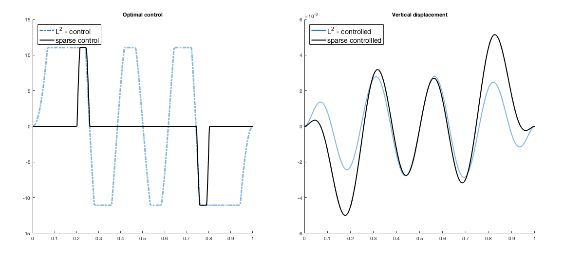
4.1. Comparison of $L^{2}$–controls with sparse controls

This example is intended to show how sparse controls act in a“located” fashion with respect to $L^{2}$–controls, which are distributed in the whole domain. In the next example, the following parameters for optimization where chosen.

$\nu=5\times 10^{-9}$,	$\eta\in[0,2.7\times 10^{-5}]$
$a=-11.05$	$b=11.05$,
$f(x)=100\sin(8\pi\,x)$	$g=0$.

We run this example in mesh with 601 nodes and compare the solutions for different values of $\eta:=0:2\times 10^{-5}$. We summarize the results in Table 1 where we show the different cost and the corresponding $L^{2}$–norm for each solution, up to the value of $\eta$ where the optimal control becomes zero. For example, the first two solutions are depicted in Figure 4.1. These plots clearly show the effect of the $L^{1}$ penalization term. Indeed, in contrast with the pure $L^{2}$–control ($\eta=0$), we observe that the sparse optimal control ( $\eta=3\times 10^{-6}$) is nonzero in two well identified sections of the beam, where both controls are active. On the other hand, we can see that the corresponding states, representing the vertical displacements are both close to 0. Although the sparse controlled state has a slightly higher amplitude, the optimal control which produces it has a much lesser $L^{2}$–norm cost.

$\eta$	Cost	$L^{2}$–norm	Null
0	1.6986e-06	9.4704	0
3e-06	6.3031e-06	3.179	530
6e-06	8.9758e-06	2.813	545
9e-06	1.1125e-05	2.5228	555
1.2e-05	1.2841e-05	2.203	564
1.5e-05	1.4146e-05	1.8141	571
1.8e-05	1.5049e-05	1.2875	576
2.1e-05	1.5553e-05	0.66013	582
2.4e-05	1.5674e-05	0.046107	596
2.7e-05	1.5677e-05	0	600

Table 1. Solution costs for different values of $\eta$

Figure 1. $L^{2}$–norm control vs sparse control and corresponding optimal states

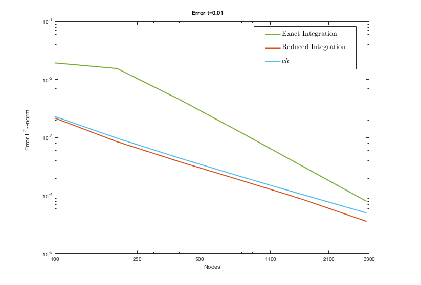
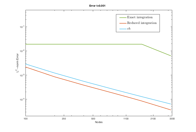
4.1.1. Testing the locking–free property

In order to illustrate the locking–free feature of our scheme, we consider two small values of the thickness: $t=10^{-2}$ and $t=10^{-3}$ (see [11], [9]). Figure 2 shows error curves in terms of the refinement parameter $N=1/h$ for controls obtained by means of the classic method, i.e., as a solution of the problem (1): $(u_{1},u_{2})$ and for the controls obtained with the superconvergence step: $(\tilde{u}_{1},\tilde{u}_{2})$. In this figure it can be clearly seen that the order of convergence is $O(h)$. For $t=0.01$, we observe that a large number of nodes is needed for the usual scheme in order to achieve the precision of the solution computed with the reduced scheme. In addition, when $t=001$ we observe the locking effect in the usual method versus the locking-free property of our scheme.

Figure 2. $L^{2}$–norm error of for optimal control for different thickness parameter

References

- [1] Douglas N. Arnold. Discretization by finite elements of a model parameter dependent problem. Numer. Math., 37(3):405–421, 1981.
- [2] Eduardo Casas. A review on sparse solutions in optimal control of partial differential equations. SeMA Journal, pages 1–26, 2017.
- [3] Eduardo Casas, Roland Herzog, and Gerd Wachsmuth. Approximation of sparse controls in semilinear equations by piecewise linear functions. Numer. Math., 122(4):645–669, 2012.
- [4] Eduardo Casas, Roland Herzog, and Gerd Wachsmuth. Approximation of sparse controls in semilinear equations by piecewise linear functions. Numer. Math., 122(4):645–669, 2012.
- [5] Casas, Eduardo, Herzog, Roland, and Wachsmuth, Gerd. Analysis of spatio-temporally sparse optimal control problems of semilinear parabolic equations? ESAIM: COCV, 23(1):263–295, 2017.
- [6] J. C. De Los Reyes, E. Loayza, and P. Merino. Second-order orthant-based methods with enriched hessian information for sparse -optimization. Computational Optimization and Applications, 67(2):225–258, Jun 2017.
- [7] Juan Carlos de los Reyes, Christian Meyer, and Boris Vexler. Finite element error analysis for state-constrained optimal control of the Stokes equations. Control Cybernet., 37(2):251–284, 2008.
- [8] C.R. Fuller, S.J. Elliott, and P.A. Nelson. Active Control of Vibration. Academic Press, 1997.
- [9] Erwin Hernández and Enrique Otárola. A locking-free FEM in active vibration control of a Timoshenko beam. SIAM J. Numer. Anal., 47(4):2432–2454, 2009.
- [10] Erwin Hernández and Enrique Otárola. A superconvergent scheme for a locking-free FEM in a Timoshenko optimal control problem. ZAMM Z. Angew. Math. Mech., 91(4):288–299, 2011.
- [11] Erwin Hernández, Enrique Otárola, Rodolfo Rodríguez, and Frank Sanhueza. Approximation of the vibration modes of a Timoshenko curved rod of arbitrary geometry. IMA J. Numer. Anal., 29(1):180–207, 2009.
- [12] A. Labuschagne, N. F. J. van Rensburg, and A. J. van der Merwe. Comparison of linear beam theories. Math. Comput. Modelling, 49(1-2):20–30, 2009.
- [13] Alessandro Macchelli and Claudio Melchiorri. Modeling and control of the Timoshenko beam. The distributed port Hamiltonian approach. SIAM J. Control Optim., 43(2):743–767 (electronic), 2004.
- [14] Otárola, Enrique and Salgado, Abner. Sparse optimal control for fractional diffusion. 2017.
- [15] Georg Stadler. Elliptic optimal control problems with -control cost and applications for the placement of control devices. Comput. Optim. Appl., 44(2):159–181, 2009.
- [16] Gerd Wachsmuth and Daniel Wachsmuth. Convergence and regularization results for optimal control problems with sparsity functional. ESAIM Control Optim. Calc. Var., 17(3):858–886, 2011.