Differentiability and Hölder spectra of a class of self-affine functions
Abstract
This paper studies a large class of continuous functions whose range is the attractor of an iterated function system consisting of similitudes. This class includes such classical examples as Pólya’s space-filling curves, the Riesz-Nagy singular functions and Okamoto’s functions. The differentiability of is completely classified in terms of the contraction ratios of the maps . Generalizing results of Lax (1973) and Okamoto (2006), it is shown that either (i) is nowhere differentiable; (ii) is non-differentiable almost everywhere but with uncountably many exceptions; or (iii) is differentiable almost everywhere but with uncountably many exceptions. The Hausdorff dimension of the exceptional sets in cases (ii) and (iii) above is calculated, and more generally, the complete multifractal spectrum of is determined.
AMS 2010 subject classification: 26A27, 26A16 (primary); 28A78, 26A30 (secondary)
Key words and phrases: Continuous nowhere differentiable function; Self-affine function; Space-filling curve; Pointwise Hölder spectrum; Multifractal formalism; Hausdorff dimension.
1 Introduction
In 1973, P. Lax [18] proved a remarkable theorem about the differentiability of Pólya’s space-filling curve, which maps a closed interval continuously onto a solid right triangle. Unlike the space-filling curves of Peano and Hilbert, which had been known to be nowhere differentiable, Lax found that the differentiability of the Pólya curve depends on the value of the smallest acute angle of the triangle. (Roughly speaking, the larger the angle, the less differentiable the function is; see Example 2.3 below.)
More than 30 years later, H. Okamoto [23] introduced a one-parameter family of self-affine functions that includes the Cantor function as well as functions previously studied by Perkins [24] and Katsuura [15]. Okamoto showed that the differentiability of his functions depends on the parameter in much the same way as the differentiability of the Pólya curve depends on the angle (though it is not clear whether Okamoto was aware of Lax’s result). See Example 2.4 below.
While Okamoto’s function and the Pólya curve are not directly related, both can be viewed as special cases of a large class of self-affine functions. The aim of this article is to study the differentiability of this class of functions, thereby generalizing the results of Lax and Okamoto, and to determine their finer local regularity behavior in the form of the pointwise Hölder spectrum.
Our class of functions is a subclass of that considered in [4] and may be described as follows. Fix , an integer , and points with . (Without loss of generality we take and .) Fix a vector . Let be contractive similitudes in satisfying the “connectivity conditions”
| (1.1) | |||
| (1.2) | |||
| (1.3) |
Put . If , we allow one or more of the to be constant, so .
Let be positive numbers with . Put for , and define the maps
so maps linearly onto a closed interval of length , and the intervals are nonoverlapping with . By a theorem of de Rham [26], there exists a unique continuous function satisfying the functional equation
| (1.4) |
Following [4], we shall call the signature of . The image is a connected, self-similar curve in satisfying . Note that (1.1)-(1.3) imply that . To avoid degenerate cases, we shall assume throughout that
| (1.5) |
Remark 1.1.
Let be the unique nonempty compact subset of such that
| (1.6) |
Since is constant on each of the intervals making up the complement of , we can think of alternatively as a continuous function from the self-similar set in onto the self-similar set in .
In each of the examples below, we take and , unless otherwise specified.
Example 1.2 (The Pólya curve).
Take . Let be a right triangle positioned as in Figure 1. We assume that , the smaller of the two acute angles of , is the angle at . The two subtriangles and in the figure are similar to ; let and be the affine transformations which map onto and , respectively. The function determined by (1.4) in this case is Pólya’s space-filling curve [25], which maps the interval onto the triangle , and .
Example 1.3 (Okamoto’s functions).
Example 1.4 (The Riesz-Nagy function).
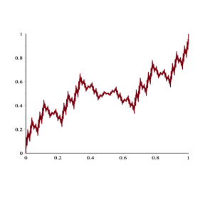
Take and , and fix a parameter , . Setting and , we obtain the Riesz-Nagy function [27, 29], one of the best known examples of a strictly increasing function whose derivative is almost everywhere zero; see Figure 3(a). In Section 9, the Riesz-Nagy functions will serve as time subordinators for other functions of the form (1.4) with .
(a)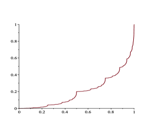 (b)
(b)
Example 1.5 (Gray code singular function).
Example 1.6 (Distribution functions of self-similar measures).
Generalizing the last two examples, let be nonoverlapping closed subintervals of , ordered so that lies to the left of when . For , let be one of the two linear contractions which map onto , and set . Let be a probability vector with for each . There is then a unique nonempty compact set such that , and there is a unique probability measure concentrated on such that
| (1.7) |
Let for ; then is of the form (1.4). To determine the parameters, write , , and set and . Let . The points (not all necessarily distinct) divide into nonoverlapping closed subintervals; let us label them from left to right. For , set if for some , and else set . Set , so if for some , and otherwise is the length of a “gap” between two successive intervals and . Note that this naturally yields examples of our set-up with some of the equal to zero. In this case, , and .
Other examples of functions satisfying (1.4) include the space-filling curves of Peano () and Hilbert (), and classical fractals such as the Koch curve and the Lévy curve [19], as well as asymmetric versions of these. However, as most of these functions are nowhere differentiable and monofractal, they are less interesting from the point of view of this article. For a comprehensive survey of space-filling curves, see [28].
Section 2 outlines the main results of the paper, illustrating them for some of the above examples. Surprisingly, the differentiability of depends on the maps only through their contraction ratios . This means that, especially when , there are many different functions in our class with the same differentiability structure, and even with the same pointwise Hölder spectrum.
We show first that the only possible finite derivative of a function of the form (1.4) under the assumption (1.5) is zero. We then generalize Lax’s and Okamoto’s theorems by showing that, depending on the values of and , is either (i) nowhere differentiable; (ii) differentiable almost nowhere, with uncountably many exceptions; or (iii) differentiable almost everywhere, with uncountably many exceptions. In cases (ii) and (iii), we compute the Hausdorff dimension of the exceptional sets. For example, in the case of Pólya’s space-filling curve we obtain that, if , the set of points where is differentiable has Hausdorff dimension , where
A large part of the paper is devoted to the pointwise Hölder spectrum – or multifractal spectrum – of . Globally, a function is said to be Hölder continuous with exponent if there is a constant such that for all and . However, this represents the “worst possible” behavior, and in general, a continuous function can at many points have substantially better regularity than the worst case.
Consider first the case of a function . For and , write if there is a constant and a polynomial of degree less than such that
| (1.8) |
The pointwise Hölder exponent of at is the number
| (1.9) |
and the pointwise Hölder spectrum of is the function , where
and denotes Hausdorff dimension. For a function , one replaces the polynomial in (1.8) by a -tuple of polynomials, each of degree less than .
Local Hölder exponents can be difficult to calculate, especially for , where, in order to show that , one must prove that no polynomial satisfying (1.8) exists. For this reason perhaps, many authors (e.g. [4, 6]) use the following, simpler definition of Hölder exponent. Write if there is a constant such that
that is, the polynomial in (1.8) is constant with value . Define
| (1.10) |
and let
We shall call the nondirectional Hölder exponent of at , and refer to the function as the nondirectional Hölder spectrum of . Observe that , but the reverse inequality may fail in general. For example, if , then (since one can take in (1.8) for all ), but . In addition, a desirable property of Hölder exponents is that they are left unchanged upon perturbation of by a smooth function . Indeed, , whereas in general.
Hölder spectra are an important analytical tool in the study of certain physical processes that exhibit a wide range of local regularity behavior, such as intermittent turbulence flows or intensity of seismic waves; see [11, 22]. They were studied by Jaffard [12, 13] for a large class of self-similar functions using wavelet methods. Jaffard’s work assumes a certain smoothness condition which our functions do not satisfy, but Jaffard and Mandelbrot [14] later modified the wavelet approach to compute the Hölder spectrum of the Pólya curve. Unfortunately, their proof omits some critical details and the final expression is incorrect. Ben Slimane [7] evaluates the multifractal spectrum of a family of self-similar functions based on binary splitting of the unit interval, which includes the Riesz-Nagy function. Both [14] and [7] use the Schauder basis, which is ideally suited to the case . But it is less clear how to identify a suitable wavelet basis for , and moreover, the theorems underlying the wavelet method are rather technical. By contrast, our approach here, while not without technicalities, is completely elementary.
Another relevant paper, by Seuret [30], uses an associated multinomial measure to compute the pointwise Hölder spectrum of Okamoto’s function. His final expression too is incorrect, due to some unfortunate transcription errors. More importantly, Seuret does not carefully address the subtlety of Hölder exponents greater than one, where the polynomial in (1.8) might be of higher degree; that is, he seems to assume without proof that . We will show that this is indeed the case for Okamoto’s function, and more generally, for all of the form (1.4) provided that and . We conjecture that regardless of the values of the and .
Theorem 2.7 gives the nondirectonal Hölder spectrum of , which is shown to satisfy the classical multifractal formalism. This is established by first obtaining an expression for at any point , which seems interesting in its own right. A crucial tool in the proof of Theorem 2.7 is the duality principle formulated in Proposition 2.10.
In Section 8 we apply our result to the multifractal spectrum of the self-similar measures from Example 1.6. We refine the classical multifractal formalism by showing that it holds also for the lower density of .
The final section of the paper connects our work to that of Seuret [30], by showing that all functions of the form (1.4) can be written as a composition of a monofractal function and an increasing function, or time subordinator.
While the work for this paper was undertaken, a closely related article by Bárány et al. [4] appeared on the arXiv. That paper considers a more general setup, in which the maps are arbitrary affine contractions on . While [4] is quite general and technically sophisticated, our restriction here to similitudes offers several advantages: (i) Bárány et al. define the pointwise Hölder exponent to be , rather than . While we are able to show that both definitions are equivalent for some functions of the form (1.4), this is far from clear for the larger class of functions in [4]; (ii) The main results of [4] require that the maps satisfy a certain positivity condition which rules out many interesting examples, including the Pólya curve; (iii) The authors of [4] succeed only in determining the “upper half” of the nondirectional Hölder spectrum. In order to obtain the full spectrum they need an additional and rather restrictive quasi-symmetry condition, which in our setting reduces to . By focusing exclusively on similitudes, we obtain the full multifractal spectrum without having to make such a symmetry assumption; (iv) Our results are more explicit, and are obtained using elementary methods. The price to pay is, of course, that our results do not cover functions such as the main example in [4], a curve introduced by de Rham. Thus, it seems that the present article and [4] complement each other quite well.
2 Main results
In what follows, we shall consider to be differentiable at if it has a well-defined finite derivative at . From now on it will be assumed without further mention that is defined by (1.4) and that (1.5) holds.
Proposition 2.1.
If is differentiable at a point , then .
Our first main result shows that the differentiability of is completely determined by the contraction ratios and .
Theorem 2.2.
-
(i)
If for each , then is nowhere differentiable;
-
(ii)
If for at least one but , then is nondifferentiable almost everywhere but at uncountably many points;
-
(iii)
If , then almost everywhere but is nondifferentiable at uncountably many points.
Example 2.3.
Applying Theorem 2.2 to the Pólya curve from Example 1.2 and using the identity , we recover Lax’s theorem, namely: (i) is nowhere differentiable when ; (ii) is nondifferentiable almost everywhere but differentiable at uncountably many points when ; and (iii) is differentiable almost everywhere but nondifferentiable at uncountably many points when . (We remark that Lax excluded the boundary cases and from his analysis; these were later dealt with by Bumby [8].)
Example 2.4.
Let be Okamoto’s function (Example 1.3). Observe that is strictly increasing, and hence differentiable almost everywhere, when . When , we have . Solving gives . We now obtain Okamoto’s result [23]: (i) is nowhere differentiable when ; (ii) is nondifferentiable almost everywhere but differentiable at uncountably many points when ; and (iii) is differentiable almost everywhere but nondifferentiable at uncountably many points when . (We remark that Okamoto did not address the boundary case , which was later settled by Kobayashi [16].)
A natural next question is: What is the Hausdorff dimension of the exceptional sets in cases (ii) and (iii) of Theorem 2.2? Let
We will consider the dimensions of and in the context of the pointwise Hölder spectrum of . Recall the definitions of and from (1.9) and (1.10). We first show that at least in the simplest cases, these two Hölder exponents are the same:
Theorem 2.5.
Assume that for , and that . Then for every .
Unfortunately, the author has been unable to extend this theorem to all functions of the form (1.4). For the remainder of this section, we will therefore focus on the (easier to analyze) nondirectional Hölder spectrum of ; that is, the function .
First, we need some additional notation. Let
Define
and let
Furthermore, let , and be the nonnegative numbers satisfying
Since , . Put
Note that .
For each , let be the unique real number such that
| (2.1) |
It is well known from multifractal theory (e.g. [10, Chapter 17]) that the function is strictly decreasing and convex, and its Legendre transform
is strictly concave on the interval , and takes the value outside this interval.
Theorem 2.6.
Assume for at least one .
-
(i)
If , then ;
-
(ii)
If , then ;
-
(iii)
If , then .
Theorem 2.7.
-
(i)
when ;
-
(ii)
is empty if , and has Lebesgue measure one otherwise;
-
(iii)
for all ;
-
(iv)
, and ;
-
(v)
The maximum value of over is attained at , and . Moreover, if , then has Lebesgue measure one.
Remark 2.8.
Before illustrating the last two theorems, we present an alternative view of that will be important for the proofs later, and that is sometimes more convenient for concrete computations. Define the function
| (2.2) |
where as usual, we set . We denote by the standard simplex in :
Let
The following equality generalizes the “maximum entropy/minimum pressure” duality observed in [5, Theorem 11].
Proposition 2.10.
For each , we have
| (2.3) |
Proposition 2.10 is geometrically pleasing: it represents as the maximum value of over the intersection of a simplex with a hyperplane. This intersection is nonempty for , as is easy to see. The characterization is especially useful when , in which case the intersection consists of a single point, and no maximization or minimization is necessary. In this case, solving the equations and gives
| (2.4) |
Observe that when , varies linearly as a function of , and takes the values and at the endpoints of . Let . Since is symmetric, we see from Theorem 2.7 and Proposition 2.10 that
| (2.5) |
In other words, a change in the values of and results only in a horizontal scaling and translation of the Hölder spectrum, but does not affect its general shape.
When , one can either compute by minimizing over , or one can apply the method of Lagrange multipliers to the constrained optimization problem in (2.3). Both approaches have their challenges in practice: the former requires one to estimate numerically first for every real ; and the latter entails solving a system of nonlinear equations in . In the special case when for , however, both methods quickly yield a fairly explicit answer. We then have simply
and setting gives that is minimized at the value of for which
| (2.6) |
(This exists and is unique, since the function is strictly increasing and tends to as , and to as , provided .) Alternatively, the method of Lagrange multipliers yields that the constrained maximum in (2.3) is attained at the point given by
and for , with as in (2.6), after which some further algebra gives
Example 2.3 (continued).
For the Pólya curve, , , and . A computation based on (2.5) yields
for . This expression, graphed in Figure 4(a) for , can be taken to correct the one given in [14].
Moreover, setting in (2.4) gives
This is increasing in on . Writing , we find that for , ; and for , .
(a)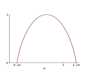 (b)
(b)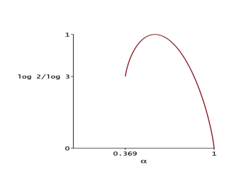
Example 2.4 (continued).
For the Hölder spectrum of Okamoto’s function we consider three cases. First, if , we have and for every outside the ternary Cantor set (and hence almost everywhere); while for every . Thus, .
If and , then and . It is intuitively clear (and easy to check) that the constrained maximum in (2.3) must be obtained when , since . A straightforward calculation shows that for ,
| (2.7) |
where
| (2.8) |
and . See Figure 4(b). At the endpoints of the multifractal spectrum, we have and . However, is uncountably large: a closer inspection reveals that it consists of those points in whose ternary expansion the digit 1 has density 1, although for each such .
Note that increases linearly from at to at . Thus, the graph of is the same for each , up to a horizontal scaling and translation.
Finally, when the calculation is the same as in the second case above, but the endpoints are reversed: , and . Here the worst regularity () is achieved when the upper density of the digit 1 in the ternary expansion of is 1, so is uncountable but of Hausdorff dimension zero. The graph of is the reverse of that in the case .
Example 2.11.
The remainder of this article is organized as follows. Section 3 introduces notation and preliminary results, including a proof of Proposition 2.10. Proposition 2.1 and Theorem 2.2 are proved in Section 4, and Theorem 2.5 is proved in Section 5. Section 6 gives the computation of for every , and Section 7 contains proofs of Theorems 2.6 and 2.7. Section 8 applies the main results to the multifractal spectrum of self-similar measures on , and Section 9 shows how functions of the form (1.4) can be written as the composition of a monofractal function and an increasing function.
3 Preliminaries
Let . For , the intersection
consists of a single point. Call a coding of if . Each point has at most two distinct codings; we shall call the lexicographically largest one the standard coding of . We write to indicate that is the standard coding of . In the special case when for each and , the standard coding of is just the expansion of in base , except that we name the digits rather than .
For , let . We will call the coding of . For and , let denote the unique interval that contains and such that the standard coding of begins with . For fixed , we enumerate the intervals from left to right as .
Let denote the set of endpoints of the intervals (, ). These are the points that have two distinct codings.
Fix , and for , let and denote the left and right endpoints, respectively, of . Thus, , and . Furthermore, let
for and , and define
provided the limit exists. Thus, is the frequency of the “digit” in the standard coding of . Since
we have
This gives, for , the useful expression
| (3.1) |
which (crucially!) does not depend on the signature .
An important tool in this paper is the following generalization of Eggleston’s theorem [9], due to Li and Dekking (see [21], Theorem 1 and eq. (35) on p. 198):
| (3.2) |
where was defined in (2.2). Generalizing Eggleston’s theorem in a different direction, Barreira et al. [5] proved, for the special case when for each and , that
| (3.3) | ||||
for real numbers . In Section 6, we will develop an expression for the nondirectional Hölder exponent which similarly involves a linear combination of the partial densities . But there is also a correction term, necessary to deal with points with exceptionally long strings of ’s or ’s in their codings. Thus, we will need a further extension of (3.3), proved in Proposition 7.6.
We end this section with a proof of Proposition 2.10.
Proof of Proposition 2.10.
Let denote the expression on the right hand side of (2.3). Assume initially that . We first show that . Since , there is a (unique) value of that minimizes . Differentiating implicitly in (2.1) and setting yields
| (3.4) |
Set for , and for . Then by (3.4), satisfies the constraints in (2.3), and
Hence, .
Conversely, let such that ; we must show that for each . By continuity of , it is enough to show this when for each . Since is decreasing in , we need to show in view of (2.1) that
| (3.5) |
Using the concavity of , we have (with all summations over )
since the last summation vanishes by definition of . Exponentiating gives (3.5). Thus, .
For , (2.3) now follows from the continuity of and in . The former is well known; the latter is a consequence of the continuity of with respect to and the continuity of with respect to and . ∎
4 Proofs of Proposition 2.1 and Theorem 2.2
In this and later sections, let
We begin with a useful lemma, whose easy proof is left to the reader.
Lemma 4.1.
Let , and suppose exists and is finite. If and are any two sequences converging to such that is bounded, then
Proof of Proposition 2.1.
Assume exists but . Then, by Lemma 4.1,
Since and , it follows that
This is possible only if for some , and then for all sufficiently large . Suppose this is the case. Fix such that . For each , let and be the left and right endpoints, respectively, of the interval . Then
so Lemma 4.1 implies
But this is impossible, since
and, for all large enough , the last fraction on the right is constant . ∎
The following lemma is a direct generalization of [18, Lemma 3].
Lemma 4.2.
Let for . If exists and for each , then .
Proof.
Suppose . Then , so
Since exists and is strictly positive, it follows that along the subsequence . Similarly considering the other digits yields . ∎
Lemma 4.3.
Suppose that for , and that
| (4.1) |
Then .
Proof.
Proof of Theorem 2.2.
To prove (ii), we assume first that . By the strong law of large numbers, for almost every and , and so
for almost every . Thus, (3.1) gives
for almost all , and hence, is differentiable almost nowhere.
The case when needs a separate argument. In this case, we view the numbers as random variables on the Lebesgue probability space with the Lebesgue (or Borel) -algebra and Lebesgue measure. Since the “digits” in the coding of are independent and identically distributed, the sums
follow a random walk with steps chosen randomly from the set , in which the expected step size is . Then, for example, the law of the iterated logarithm implies that for almost all ,
Exponentiating and using (3.1), it follows that is differentiable almost nowhere.
The claim that at uncountably many if for some will follow once we prove Theorem 2.6.
5 Proof of Theorem 2.5
In this section we assume the hypotheses of Theorem 2.5: for each , and . Note that is then simply the set of all -adic rational numbers in .
Proof of Theorem 2.5.
Fix , and assume with . Let be the greatest integer strictly less than . Thus, there are polynomials of degree at most and a constant such that
| (5.1) |
where we write . We need to show that for . Aiming for a contradiction, assume that this is not the case. Write
For each , set if is constant, and otherwise, set . Note that at least one is finite; let . We can divide by in (5.1) to obtain
| (5.2) |
since
for . Observe that (5.2) is a rather strong statement. For instance, if it says that has a well-defined nonzero derivative at , which is impossible in view of Proposition 2.1. Thus, we must have .
Case 1. Assume first that , say . It will be sufficient to consider . Since the graph of on the interval is an affine copy of the full graph of , we can and do assume without loss of generality that . For each , (5.2) gives
so that
Letting
for and , it follows that
| (5.3) |
On the other hand, for it follows from (1.4) that . In particular, setting in (5.3) gives
But similarly we have , so setting in (5.3) we obtain
Thus, . But this is impossible, since and the function is strictly convex on for .
Case 2. Assume now that . We initially assume also that for each . Note that is a product of some combination of the , and is therefore nonzero. Define the set
It is easy to see that
and therefore has no limit points in .
Define the map by , and denote by the th iterate of . Since is not -adic rational, there is a number and a subsequence of such that . To avoid notational clutter, we shall for the remainder of the proof suppress the index and simply write instead of . By continuity of ,
Here and in what follows, convergence takes place along the subsequence as . Assume initially that . Write . Then , so
Thus, (5.2) implies
| (5.4) |
Next, for we have
and so
| (5.5) |
Write . Then
| (5.6) |
where
Combining (5.4), (5.5) and (5.6), we obtain
and so
since and the function is strictly convex on . However, , and since does not have a limit point in , it follows that (for each fixed ) is eventually constant, say
But then , and , contradicting again that does not have a limit point in .
6 Calculation of
In this section we derive a precise (but somewhat technical) expression for in terms of the coding of . Assume without loss of generality that
| (6.1) |
(If this does not hold, simply switch the roles of the digits and everywhere in what follows.) Let
| (6.2) |
Note that . For , define the “look back” run length
| (6.3) |
or if . For , let
There are three essentially different cases to consider. We deal with the case separately, in Theorem 6.5. If , then is constant on for some , and . The critical case, addressed in Theorem 6.1 below, is when and . We make the convention that and .
Theorem 6.1.
Assume (6.1), and let .
-
(i)
There is a unique number such that
(6.4) and if , then .
-
(ii)
Suppose . Let
where . Then there is a unique number such that
(6.5) Moreover, , and .
Corollary 6.2.
Assume (6.1). Let . If exists for and , then
| (6.6) |
Proof.
The proof of Theorem 6.1 uses the following lemmas.
Lemma 6.3.
Under the respective hypotheses of Theorem 6.1, the numbers and exist and are unique, and lie in .
Proof.
We demonstrate the existence and uniqueness of in case (ii); the proof concerning is more straightforward.
Assume . We first show that is well defined. Since , there is at least one index such that , as otherwise we would have . We may then assume (since we are going to let ) that with chosen as above, so that . By the definition of in (6.3), and so . If furthermore , then as well and so is well defined. If (in which case ), then and so . Thus, in all cases is well defined and as a result, is well defined.
Writing the expression in square brackets in (6.5) as , we have and . Thus for each , exists and moreover, is strictly increasing and continuous in , since the of a sequence of linear functions is convex, and hence, continuous. Furthermore, we claim that
| (6.7) |
This is clear when . Otherwise, by (6.2), , and since for and , we have for each ,
Dividing by and taking gives the first inequality in (6.7). The second inequality is clear. Therefore, has a unique zero in . ∎
Lemma 6.4.
Let and have codings and , respectively. Let . Let and . If either or , then for .
Proof.
We have and . If, say, and , then and can each be either or (depending on the values of and ), but in all cases. A similar conclusion holds if and , with replaced by . If , then and consist of alternating ’s and ’s. (For instance, if and is odd, then and or vice versa.) Finally, if and , then or . Thus, in all cases, for . ∎
Proof of Theorem 6.1.
Note that
For an interval , let be the oscillation of over . Assume initially that , so that
| (6.8) |
(a) We first show that when . Let
Fix . Let , and let be the largest integer such that
| (6.9) |
Then , so there is an absolute constant such that ; we write this as .
If , then we have simply
| (6.10) |
as .
Assume therefore that . Let be the integer such that . Let be the coding of the adjacent interval . We sort out the cases in which the length of is comparable to . Define and as in Lemma 6.4. Since , Lemma 6.4 implies that for each . But then , so , and moreover, . Thus,
| (6.11) |
as in (6.10). The argument for is similar. Hence, when .
(b) We next show that when . Fix ; then certainly , so we can follow the argument under (a) up to the point where Lemma 6.4 is used. Define , and as in Lemma 6.4. If , then obviously for each . By Lemma 6.4, the same is true if . In these cases, we get (6.11) in the same way as before and we are done.
From now on we can, therefore, assume that , and . Since , .
Case 1. Suppose . Then and for , so . Now , and
Let be the largest integer (possibly negative) such that
Then
and so
| (6.12) |
Note that by (6.9). Therefore, the interval is adjacent to and has length . Moreover,
At this point, the fact that and implies that , so with , we have . Therefore, if , then and so , which means we simply have (6.10) again.
Case 2. Suppose . This case is more straightforward. We reverse the roles of the “digits” and . If , let be the largest integer such that (or if ). Put , and note that . Now we similarly find a basic interval adjacent to and with
But, since , we simply have for a suitable constant , and we again obtain (6.13).
The argument for is entirely similar. We have thus shown that .
(c) Next, we show that . Let ; then
where we recall that . Since
it follows that
Hence, .
(d) Finally, we show that when . Fix . Given , let , and let again be the integer such that . If , there is nothing to show, so assume . This implies . Also assume , so . (Otherwise there is again nothing to show.) Then either of the intervals and has length ; assume without loss of generality that this interval is .
Note that
| (6.14) |
Let be the largest integer such that
Then by (6.14). Let be the integer such that and have the same left endpoint. We have
| (6.15) |
Furthermore,
Let be the right endpoint of . Since , we have , and as in the first half of the proof we obtain
Recall also that . Hence, since ,
| (6.16) |
Now write
Note that
in view of (6.15). Therefore, (6.16) implies
Hence, .
(e) So far we had assumed that . However, if , then and our assumption that for each implies that for every , so we always have in the analysis above, and . This completes the proof. ∎
Since is a countable set, it plays no role in the determination of the pointwise Hölder spectrum of . But, for completeness, we determine for as well. Each such has two different codings, either (i) both ending in ; (ii) both ending in ; (iii) one ending in and one in ; or (iv) both ending in , either in sync or one step out of phase. (Possibility (iv) occurs when .)
Theorem 6.5.
Assume (6.1), and let . Assume neither coding of contains a digit from .
-
(i)
If at least one coding of ends in , then ;
-
(ii)
If both codings of end in , then ;
-
(iii)
If both codings of end in , then .
Proof.
Assume has one coding ending in and one ending in . Say the coding “from the right” is the one ending in ; that is, for some interval and all , is the left endpoint of . Let , and let be the integer such that . Then
for a suitable constant depending only on . For we similarly have . As a result, . Equality follows by considering the sequence .
The other cases are proved similarly. ∎
Remark 6.6.
(a) It follows from Theorem 6.5 that the expression (6.6) is valid also for , provided that in case (i) we use a coding for ending in .
(b) If both codings of contain a digit from , then . If only one coding of contains a digit from , then the other coding determines as in cases (i)-(iii) of Theorem 6.5 (suitably modified).
7 Proofs of Theorems 2.6 and 2.7
The lower bound for the dimension of is straightforward.
Lemma 7.1.
Let . Then .
Proof.
Proving that is rather more difficult. We first develop a few technical lemmas. Without loss of generality we assume (6.1). For brevity, write
where we set . In the following definition and lemmas, assume is given by (6.8). For , and , define the set of partitions
Lemma 7.2.
Suppose . Then for every , every , every sufficiently large and every ,
where is the largest integer such that .
Proof.
Let . Put , for , and . Then , and . Moreover,
for all sufficiently large , where the first inequality follows since and , by definition of . Thus, for all large enough . Furthermore, by the definition of , , and so . Hence,
and
again by definition of . Thus, the desired inequality follows. ∎
Lemma 7.3.
Suppose . Then for every , every , every sufficiently large and every ,
where is the smallest integer such that , and .
Proof.
Let . Put , for , and . Then , and . Moreover, as in the proof of Lemma 7.2,
for all sufficiently large . Now the definition of implies , so
and hence,
for all large enough , keeping in mind that . Thus, , and it follows that for all sufficiently large . Furthermore (since ),
and
again by definition of . The desired inequality follows. ∎
Lemma 7.4.
Let , and let be nonnegative integers with . Put for . Then
where we use the convention .
Proof.
We use the following precise version of Stirling’s approximation:
| (7.1) |
Let . Using that , we obtain from (7.1)
as required. ∎
Next, let be the vector defined by for , and for . Then , and
Note also that, if , then
so the half space does not contain the point . For , define the subsimplex
Lemma 7.5.
Let and suppose . Then the maximum value of over is attained on the hyperplane .
Proof.
Using Lagrange multipliers one can show that has only one critical point in , which is the absolute maximum at . Since this point lies outside , the maximum of over is attained on the boundary of , where we use the relative topology of the -dimensional hyperplane containing . But it is easy to see that the restriction of to cannot have a local maximum on the boundary of , because has infinite gradient there. Hence, the maximum value of on is attained on the set . ∎
Proposition 7.6.
Let .
-
(i)
If , then ;
-
(ii)
If , then .
Proof.
By Lemma 7.1, is a lower bound for the Hausdorff dimension of each of the above two sets, since they both contain . The proof that is also an upper bound is more involved.
Suppose , and consider the set . Note that . If , then . Assume therefore that . Without loss of generality, we may also assume (6.1).
Assume first that . For , define
| (7.2) |
Note that as .
Given , let . Fix , and choose small enough so that in fact, and . (This is possible by the discussion preceding Lemma 7.5.) Set .
For , put for , and note that , since the condition forces those ’s with to be zero. By Lemma 7.4,
| (7.3) |
and the key is that the product inside the th power is less than 1:
Since is compact, it follows that
| (7.4) |
Now fix . If , then there is in integer such that
by Theorem 6.1, so the -tuple lies in , where . There are
basic intervals of level whose points satisfy and for , and each has length . Let denote -dimensional Hausdorff measure. Then (since is countable),
We now consider two cases.
Case 1. Suppose . For each and , let be as in Lemma 7.2. Then
where . Since for and , Lemma 7.2, (7.3) and (7.4) give
Case 2. Suppose . For each and , let be as in Lemma 7.3. Then
for all large enough , so Lemma 7.3, (7.3) and (7.4) give
This concludes the proof that in case .
When the proof is much simpler, since and so the term in (6.5) involving vanishes, leading to a much more straightforward covering argument.
Likewise, the proof of (ii) is much easier, because , where is defined as in Theorem 6.1, and so we have . This last set is straightforward to cover in a manner similar to the above.
Alternatively, (ii) may be deduced quickly from the main result of [20]. ∎
Proof of Theorem 2.7.
(ii) If , then for every by Theorems 6.1 and 6.5. If , then the standard coding of almost every has at least one digit in , and so almost everywhere.
(iii) Fix . By Lemma 7.1, . The reverse inequality follows from Proposition 7.6: If , use that ; and if , use that .
Proof of Theorem 2.6.
Assume throughout that for at least one .
(i) Suppose . Then in particular, for each , and
Moreover, for at least one , so . Since
Proposition 7.6(ii) and the continuity of imply .
(ii) Suppose . Then , so . Thus, . By a straightforward continuity argument, as . Since
| (7.5) |
we conclude that .
8 Multifractal formalism for self-similar measures
In this section, consider a self-similar measure on defined as in Example 1.6. We are interested in the upper and lower local dimension of at a point , defined by
where . If , we denote the common value by . Let
It has been known for some time (see [3]) that
where is the unique number satisfying . The question is, whether in the above equation we can replace with or . The author could not find an answer to this question in the literature, but in any case, it follows immediately from our results that the answer is affirmative for :
Corollary 8.1.
Proof.
Unfortunately, the results and analysis of this paper have no direct implications for the Hausdorff dimension of . (However, from the main result of [20] it follows that for all .) It also should be noted that we obtain only for self-similar measures in , and our method has no obvious generalization to higher dimensions.
9 Monofractal functions and time subordinators
Return now to the general function of the form (1.4), with arbitrary , , contraction ratios and , and signature . Seuret [30] gave conditions under which a continuous function can be written as the composition of a monofractal function and an increasing function, or time subordinator. We show here, as a consequence of our main results, that for of the form (1.4) such a decomposition is always possible.
Let be the solution of . There is a unique monotone increasing function of the form (1.4) satisfying , , with , and for , and .
It is a direct consequence of Theorems 6.1 and 6.5 that
so the nondirectional Hölder spectrum of is just a horizontal scaling of that of : . When and , we may replace with and with in the above.
Now define by , where for . Since and are continuous, . Furthermore, is also of the form (1.4), with , and , where is the index of the the th nonzero entry of the vector . It follows immediately from Theorem 6.1 that is monofractal with constant Hölder exponent for all .
Since is monotone increasing, it can be viewed as a time subordinator for the function . For example, in the case of the Pólya curve we have , and the subordinator is the Riesz-Nagy function with parameter . The function in this case is a reparametrization of the Pólya curve which fills equal areas in equal time, and has constant Hölder exponent . Similarly, the time subordinator for Okamoto’s function with parameter (i.e. the non-monotone case) is the Okamoto function with parameter , where is the unique root of . (This example was given by Seuret.) Finally, observe that the time subordinator is always a singular function, in view of Proposition 2.1.
Acknowledgment
The author wishes to thank Prof. Lars Olsen for bringing the paper [20] to his attention, Prof. Zoltán Buczolich for a helpful discussion about pointwise Hölder exponents, and the referee for his or her careful reading of the paper and for suggesting several improvements to the presentation.
References
- [1] P. C. Allaart, The infinite derivatives of Okamoto’s self-affine functions: an application of -expansions. J. Fractal Geom. 3 (2016), no. 1, 1–31.
- [2] P. C. Allaart, Differentiability of a two-parameter family of self-affine functions. J. Math. Anal. Appl. 450 (2017), no. 2, 954–968.
- [3] M. Arbeiter and N. Patzschke, Random self-similar multifractals. Math. Nachr. 181 (1996), 5–42.
- [4] B. Bárány, G. Kiss and I. Kolossváry, Pointwise regularity of parameterized affine zipper fractal curves. Preprint, arXiv:1608.04558.
- [5] L. Barreira, B. Saussol and J. Schmeling, Distribution of frequencies of digits via multifractal analysis. J. Number Theory 97 (2002), 410–438.
- [6] T. Bedford, Hölder exponents and box dimension for self-affine fractal functions. Constr. Approx. 5 (1989), 33–48.
- [7] M. Ben Slimane, Multifractal formalism for selfsimilar functions expanded in singular basis. Appl. Comput. Harmon. Anal. 11 (2001), 387–419.
- [8] R. T. Bumby, The differentiability of Pólya’s function. Adv. Math. 18 (1975), 243–244.
- [9] H. Eggleston, The fractional dimension of a set defined by decimal properties. Quart. J. Math. Oxford Ser. 20 (1949), 31–36.
- [10] K. J. Falconer, Fractal Geometry. Mathematical Foundations and Applications, 2nd Edition, Wiley (2003)
- [11] U. Frisch and G. Parisi, Fully developed turbulence and intermittency, in Proc. Enrico Fermi, International Summer School in Physics, North Holland, Amsterdam (1985), 84-88.
- [12] S. Jaffard, Multifractal formalism for functions part I: results valid for all functions. SIAM J. Math. Anal. 28 (1997), no. 4, 944–970.
- [13] S. Jaffard, Multifractal formalism for functions part II: self-similar functions. SIAM J. Math. Anal. 28 (1997), no. 4, 971–998.
- [14] S. Jaffard and B. B. Mandelbrot, Local regularity of nonsmooth wavelet expansions and application to the Polya function. Adv. Math 120 (1996), 265–282.
- [15] H. Katsuura, Continuous nowhere-differentiable functions - an application of contraction mappings. Amer. Math. Monthly 98 (1991), no. 5, 411–416.
- [16] K. Kobayashi, On the critical case of Okamoto’s continuous non-differentiable functions. Proc. Japan Acad. Ser. A Math. Sci. 85 (2009), no. 8, 101–104.
- [17] Z. Kobayashi, Digital sum problems for the Gray code representation of natural numbers. Interdiscip. Inform. Sci. 8 (2002), 167–175.
- [18] P. D. Lax, The differentiability of Pólya’s function. Adv. Math. 10 (1973), 456–464.
- [19] P. Lévy, Les courbes planes ou gauches et les surfaces composées de parties semblables au tout. J. Ecole Polytechn. (1938), 227-247, 249-291.
- [20] J. Li, M. Wu and Y. Xiong, Hausdorff dimensions of the divergence points of self-similar measures with the open set condition. Nonlinearity 25 (2012), 93–105.
- [21] W. Li and F. M. Dekking, Hausdorff dimension of subsets of Moran fractals with prescribed group frequency of their codings. Nonlinearity 16 (2003), 187–199.
- [22] B. Mandelbrot, Intermittent turbulence in self-similar cascades: Divergence of high moments and dimension of the carrier. J. Fluid Mech. 62 (1974), 331.
- [23] H. Okamoto, A remark on continuous, nowhere differentiable functions. Proc. Japan Acad. Ser. A Math. Sci. 81 (2005), no. 3, 47–50.
- [24] F. W. Perkins, An elementary example of a continuous non-differentiable function. Amer. Math. Monthly 34 (1927), 476–478.
- [25] G. Pólya, Über eine Peanosche Kurve. Bull. Acad. Sci. Cracovie A (1913), 305-313.
- [26] G. de Rham, Sur quelques courbes definies par des équations fonctionnelles. Univ. e Politec. Torino. Rend. Sem. Mat. 16 (1957), 101–113.
- [27] F. Riesz and B. Sz.-Nagy, Functional Analysis, Ungar, New York, 1955.
- [28] H. Sagan, Space-filling curves, Springer-Verlag, New York, 1994.
- [29] R. Salem, On some singular monotonic functions which are strictly increasing. Trans. Amer. Math. Soc. 53 (1943), 427–439.
- [30] S. Seuret, On multifractality and time subordination for continuous functions. Adv. Math. 220 (2009), no. 3, 936–963.