An Online Learning Approach to Buying and Selling Demand Response

Abstract

We adopt the perspective of an aggregator, which seeks to coordinate its purchase of demand reductions from a fixed group of residential electricity customers, with its sale of the aggregate demand reduction in a two-settlement wholesale energy market. The aggregator procures reductions in demand by offering its customers a uniform price for reductions in consumption relative to their predetermined baselines. Prior to its realization of the aggregate demand reduction, the aggregator must also determine how much energy to sell into the two-settlement energy market. In the day-ahead market, the aggregator commits to a forward contract, which calls for the delivery of energy in the real-time market. The underlying aggregate demand curve, which relates the aggregate demand reduction to the aggregator’s offered price, is assumed to be affine and subject to unobservable, random shocks. Assuming that both the parameters of the demand curve and the distribution of the random shocks are initially unknown to the aggregator, we investigate the extent to which the aggregator might dynamically adapt its offered prices and forward contracts to maximize its expected profit over a time window of $T$ days. Specifically, we design a dynamic pricing and contract offering policy that resolves the aggregator’s need to learn the unknown demand model with its desire to maximize its cumulative expected profit over time. In particular, the proposed pricing policy is proven to incur a regret over $T$ days that is no greater than $O(\log(T)\sqrt{T})$.

1 Introduction

The large scale utilization of demand response (DR) resources has the potential to substantially improve the reliability and efficiency of electric power systems. Accordingly, several state and federal mandates have been established to facilitate the integration of demand response resources into wholesale electricity markets. For example, FERC Order 719 mandates that Independent System Operators (ISOs) permit the direct sale of energy produced by DR resources into wholesale electricity markets [2]. However, as individual residential customers often posses insufficient capacity to participate in such markets directly, there emerges the need for an intermediary, or aggregator, with the ability to coordinate the demand response of large numbers of residential customers for direct sale into the wholesale electricity market. Such is consistent with the growing multitude of ISO and utility-run DR programs, which require that aggregated DR resources have a minimum load curtailment capability. For example, the Proxy Demand Resource (PDR) program operated by the California ISO has minimum capacity requirement of 100 kW, while the Day-Ahead Demand Response Program (DADRP) operated by the New York ISO has a more stringent capacity requirement of one MW.

In this paper, we adopt the perspective of an aggregator, which seeks to coordinate its purchase of an aggregate demand reduction from a fixed group of residential electricity customers, with its sale of the aggregate demand reduction into a two-settlement wholesale energy market. Formally, this amounts to a two-sided optimization problem, which requires the aggregator to balance the cost it incurs in procuring a reduction in demand from participating customers against the revenue it derives from its sale of the (a priori uncertain) demand reduction into the wholesale energy market.

More specifically, we consider the setting in which the aggregator purchases demand reductions from its customers using a non-discriminatory, posted price mechanism. That is to say, each participating customer is payed for her reduction in electricity demand according to a uniform per-unit energy price determined by the aggregator. Pricing mechanisms of this form fall within the more general category of DR programs that rely on peak time rebates (PTR) as incentives for demand reduction. Prior to its realization of the aggregate demand reduction, the aggregator must also determine how much energy to sell into the two-settlement energy market. In the day-ahead (DA) market, the aggregator commits to a forward energy contract, which calls for delivery of the contracted energy in the real-time (RT) market. If the realized reduction in demand exceeds (falls short of) the forward contract, then the difference is sold (bought) in the RT market. Therefore, in order to maximize its profit, the aggregator must co-optimize the DR price it offers its customers with the forward contract that it commits to in the wholesale energy market, as the former determines its ability to deliver the latter.

There are a variety of challenges that the aggregator faces in operating such DR programs. The most basic challenge is the prediction of how customers will adjust their aggregate demand in response to different DR prices, i.e., the aggregate demand curve. If the offered price is too low, consumers may be unwilling to curtail their demand; if the offered price is too high, the aggregator pays too much and gets more reduction than is needed. As the aggregator is initially ignorant to the customers’ aggregate demand curve, the aggregator must attempt to learn a model of customer behavior over time through repeated observations of demand reductions in response to the DR prices that it offers. Simultaneously, the aggregator must jointly adjust its DR prices and forward contract offerings in such a manner as to facilitate profit maximization over time. As we will later show, such tasks are intimately related, and give rise to a fundamental trade-off between the need to learn (explore) and earn (exploit).

Contribution:  In this paper, we study the setting in which the aggregator is faced with an aggregate demand curve that is affine in price, and subject to unobservable, additive random shocks. We assume that both the parameters of the demand curve and the probability distribution of the random shocks are fixed, but initially unknown to the aggregator. Faced with such ignorance, we explore the extent to which the aggregator might dynamically adapt its posted DR prices and offered contracts to maximize its expected profit over a time frame of $T$ days. Specifically, we design a causal pricing and contract offering policy that resolves the aggregator’s need to learn the unknown demand model with its desire to maximize its cumulative expected profit over time. The proposed pricing policy is proven to exhibit regret (relative to an oracle) over $T$ days that is at most $O(\log(T)\sqrt{T})$. In addition, the proposed policy is proven to generate a sequence of posted DR prices and forward contracts that converge to the oracle optimal DR price and forward contract in the mean square sense.

Related Work:   There is a large body of literature in power systems concerned with the aggregation and coordination of flexible demand-side resources to optimize certain economic objectives that an aggregator might encounter in wholesale energy or ancillary service markets. In such settings, the aggregator will typically exercise control over the consumption of participating demand-side resources using either (1) a direct load control mechanism whereby the aggregator can directly regulate the consumption of participating load resources according to a pre-specified contract [3, 4, 5, 6, 7, 8, 9, 10, 11, 12, 13]; or (2) an indirect load control mechanism whereby customers adjust their load in response to price signals or incentives offered by the aggregator (e.g., time-of-use pricing, peak time rebates, etc.) [14, 15, 16, 17, 18, 19, 20, 21].

The literature—as it relates to the problem of co-optimizing an aggregator’s (two-sided) transactions between end-use customers and the wholesale market—is much less developed. Campaigne et al. [22] consider a two-sided market model that is perhaps closest in nature to the one considered in this paper. Specifically, the authors adopt a mechanism design approach to the procurement of load reductions from customers, where customers are rationed and remunerated according to their self-reported types. In this paper, we adopt a posted price approach to the procurement of demand reductions from customers. This is in sharp contrast to the mechanism design approach of [22], as it gives rise to the need to learn customers’ types (i.e., demand functions) over time from measured data. From a practical standpoint, there are a variety of reasons as to why a posted price approach might be preferable to the mechanism design approach advocated by Campaigne et al. [22], not the least of which pertains to the simplicity and ease of implementation of posted pricing schemes. We refer the reader to [25] for a detailed discussion surrounding the advantages and disadvantages of such an approach in the context of online marketplaces. To the best of our knowledge, this paper is the first to analyze the use of a posted pricing scheme by an aggregator participating in such two-sided markets.

Organization:  The remainder of the paper is organized as follows. In Section 2, we formulate the aggregator’s profit maximization problem. In Section 3, we propose a recursive estimation scheme to facilitate the online learning of the unknown demand model. In Section 4, we propose an adaptive pricing and contract offering policy for the aggregator, and provide a theoretical analysis that establishes a sublinear growth rate of the regret incurred by the policy. In Section 5, we illustrate the performance of our proposed policy with a numerical case study. A table listing the pertinent notation used in this paper can be found in the Appendix to the paper. Detailed proofs of all formal results can be found in the Appendix to the paper.

2 Model

We adopt the perspective of an aggregator who seeks to purchase demand reductions from a fixed group of $N$ customers for sale into a two-settlement wholesale energy market. The market is assumed to repeat over multiple time periods (e.g., days) indexed by $t=1,2,\ldots$. The actions taken by the both aggregator and customers are described in detail in the following subsections, and concisely summarized in Table 1.

2.1 Two-Settlement Market Model

At the beginning of each day $t$, the aggregator commits to a forward contract for energy in the day-ahead (DA) market in the amount of $Q_{t}$ (kWh). The forward contract is remunerated at the DA energy price. The forward contract calls for delivery in the real-time (RT) market. If the energy delivered by the aggregator (i.e., the aggregate demand reduction) falls short of the forward contract, the aggregator must purchase the shortfall in the RT market at the shortage price. If the energy delivered exceeds the forward contract, the aggregator must sell the excess supply in the RT market at the overage price. Naturally, the wholesale energy prices will vary from day to day. We denote the wholesale energy prices (measured in $/kWh) on day $t$ by:

• $\pi_{t}$, DA energy price,

• $\pi^{-}_{t}$, RT shortage price,

• $\pi^{+}_{t}$, RT overage price.

We make several standard assumptions regarding the aggregator’s actions and the determination of energy prices in the wholesale market. First, we assume that the aggregator’s maximum demand curtailment capacity is small relative to the total volume of the DA energy market. Under this assumption, it is reasonable to assume that the aggregator cannot appreciably affect price. Accordingly, we assume that the aggregator behaves as a price taker in the DA energy market, and model the DA energy price $\pi_{t}$ as fixed and known at the outset of each period $t$. Second, as the RT imbalance prices $(\pi^{-}_{t},\pi^{+}_{t})$ are not known to the aggregator at the time of committing to a forward contract in the DA market, we model them as random variables whose expected values are denoted by

$$\mu^{-}:=\mathbb{E}[\pi^{-}_{t}]\quad\text{and}\quad\mu^{+}:=\mathbb{E}[\pi^{+}_{t}]$$

for each period $t$. Note that while we allow the RT imbalance price realizations to vary across time, we require that their expected values be time invariant. We make the following technical assumption in a similar manner to [22].

Assumption 1

The DA energy price satisfies $\pi_{t}>0$ and $\mu^{+}<\pi_{t}<\mu^{-}$ on each day $t$.

Assumption 1 serves to facilitate clarity of exposition and analysis in the sequel, as it will preserve the concavity of the aggregator’s expected profit function (2). Moreover, this assumption eliminates the possibility of perverse market outcomes in which the aggregator offers forward energy contracts with the explicit intention of deviating from the contract in the RT market.

2.2 Demand Response Model

In order to fulfill its forward contract commitment $Q_{t}$ on day $t$, the aggregator must elicit an aggregate reduction in demand from its customers. It does so by broadcasting a uniform DR price $p_{t}\geq 0$, to which each customer $i$ responds with a reduction in demand in the amount of $D_{it}$ (kWh), thereby entitling each customer $i$ to receive a payment of $p_{t}D_{it}$. We note that implicit in this model is the assumption that each customer’s reduction in demand is measured against a predetermined baseline. The question as to how to accurately estimate baseline demand is a challenging and active area of research [26, 27, 28, 29]. The generalization of our model to accommodate the endogenous estimation of a priori uncertain customer baselines is left as a direction for future research.

Actor(s)	Decision	Description
Aggregator	$Q_{t}$	In the day-ahead (DA) market on day $t$, the
		aggergrator commits to a forward energy contract
		$Q_{t}$, which calls for delivery over pre-specified
		interval of time in the real-time (RT) market.
Aggregator	$p_{t}$	Prior to delivery in the RT market, the aggregator
		broadcasts a uniform price $p_{t}$ for demand reduction
		to all customers participating in the DR program.
Customers	$D_{t}$	In the RT market, participating customers respond
		to the aggregator’s offered price $p_{t}$ by reducing
		their aggregate demand by an amount $D_{t}$.

Table 1: Description and timing of actions taken by the aggregator and customers.

We model the response of each customer $i$ to the posted price $p_{t}$ at time $t$ according to the affine function

$$D_{it}=a_{i}p_{t}+b_{i}+\varepsilon_{it},\quad\text{for}\ \ i=1,\dots,N,$$

where $a_{i}\in\mathbb{R}$ and $b_{i}\in\mathbb{R}$ are customer $i$’s idiosyncratic demand model parameters, and $\varepsilon_{it}$ is an unobservable demand shock, which we model as a zero-mean random variable. We assume that both the model parameters $a_{i}$ and $b_{i}$, and the probability distribution function of the demand shock are initially unknown to the aggregator. Clearly, the aggregate demand reduction $D_{t}:=\sum_{i=1}^{N}D_{it}$ satisfies the affine relationship

$$D_{t}=ap_{t}+b+\varepsilon_{t},$$ (1)

where the aggregate demand model parameters and shock are defined as $a:=\sum_{i=1}^{N}a_{i}$, $b:=\sum_{i=1}^{N}b_{i}$, and $\varepsilon_{t}:=\sum_{i=1}^{N}\varepsilon_{it}$, respectively. In the sequel, we will occasionally denote the tuple of aggregate demand parameters according to $\theta:=(a,b)$.

We assume throughout the paper that $a\in\left[\underline{a},\overline{a}\right]$ and $b\in\left[0,\overline{b}\right]$, where the parameter bounds $\underline{a}$, $\overline{a}$, and $\overline{b}$ are assumed to be known and satisfy $0<\underline{a}\leq\overline{a}<\infty$ and $0\leq\overline{b}<\infty$. Such assumptions are natural, as they ensure a bounded and positive price elasticity of aggregate demand, and that reductions in aggregate demand are guaranteed to be nonnegative in the absence of demand shocks. In addition to the following technical assumption, we also assume that the sequence of aggregate demand shocks $\{\varepsilon_{t}\}$ are independent and identically distributed (IID) random variables, which are mutually independent from the RT imbalance prices $\{\pi^{+}_{t}\}$ and $\{\pi^{-}_{t}\}$.

Assumption 2

The aggregate demand shock $\varepsilon_{t}$ takes values in the interval $[\underline{\varepsilon},\overline{\varepsilon}]$. Moreover, its cumulative distribution function $F$ is bi-Lipschitz over this range. Namely, there exists a real constant $L\geq 1$, such that for all $x,y\in[\underline{\varepsilon},\overline{\varepsilon}]$, it holds that

$$\frac{1}{L}\left|x-y\right|\leq\left|F(x)-F(y)\right|\leq L\left|x-y\right|.$$

The assumption that the aggregate demand shock takes bounded values is natural, given the physical limitation on the range of values that demand can take. We also note that we do not require the aggregator to have explicit knowledge of the parameters specified in Assumption 2 beyond the assumption of their boundedness.

2.3 Aggregator Profit

The expected profit derived by the aggregator during period $t$ given a fixed forward contract $Q_{t}$ and price $p_{t}$ is determined by

$$r_{t}(Q_{t},p_{t}):=\pi_{t}Q_{t}+\mathbb{E}\left[\pi^{+}_{t}[D_{t}-Q_{t}]^{+}-\pi^{-}_{t}[Q_{t}-D_{t}]^{+}-p_{t}D_{t}\right],$$

where $[x]^{+}:=\max\{0,x\}$ for all $x\in\mathbb{R}$. Given our previous assumption that the demand shocks $\{\varepsilon_{t}\}$ are mutually independent from the RT imbalance prices $\{\pi^{+}_{t}\}$ and $\{\pi^{-}_{t}\}$, the expected profit function simplifies to

$$r_{t}(Q_{t},p_{t})=\pi_{t}Q_{t}+\mu^{+}\mathbb{E}\left[[D_{t}-Q_{t}]^{+}\right]-\mu^{-}\mathbb{E}\left[[Q_{t}-D_{t}]^{+}\right]-\mathbb{E}\left[p_{t}D_{t}\right].$$ (2)

Here, expectation is taken with respect to the random demand shock $\varepsilon_{t}$.

We define the oracle optimal contract and price as

$$(Q^{*}_{t},p^{*}_{t}):=\mathop{\rm argmax}\{r_{t}(Q,p):(Q,p)\in\mathbb{R}^{2}\}.$$ (3)

That is to say, $(Q^{*}_{t},p^{*}_{t})$ denote the forward contract and DR price, which jointly maximize the aggregator’s expected profit on day $t$ given perfect knowledge of the demand model. It is straightforward to calculate the oracle optimal contract and price from the first-order optimality condition associated with problem (3), as the expected profit criterion (2) is guaranteed to be jointly concave in its arguments $(Q_{t},p_{t})$ given that satisfaction of Assumption 1. The closed-form expressions for the oracle optimal contract and price are given in the following lemma.

Lemma 1 (Oracle Optimal Policy)

For each period $t\geq 1$, the oracle optimal contract $Q^{*}_{t}$ and price $p^{*}_{t}$ are given by

$$Q^{*}_{t} =\frac{1}{2}\left(a\pi_{t}+b\right)+F^{-1}(\alpha_{t}),$$ (4)

$$p^{*}_{t} =\frac{1}{2}\left(\pi_{t}-\frac{b}{a}\right),$$ (5)

where

$$\alpha_{t}:=\frac{\pi_{t}-\mu^{+}}{\mu^{-}-\mu^{+}}.$$

Here, $F^{-1}(\alpha_{t}):=\inf\{x\in\mathbb{R}:F(x)\geq\alpha_{t}\}$ denotes the $\alpha_{t}$-quantile of the random demand shock $\varepsilon_{t}$. Assumption 1 ensures that the price ratio $\alpha_{t}$ is a valid probability, i.e., $\alpha_{t}\in(0,1)$. It is also worth noting that the oracle optimal contract can be equivalently rewritten as $Q^{*}_{t}=ap^{*}_{t}+b+F^{-1}(\alpha_{t})$. It follows that $Q^{*}_{t}$ can be interpreted as the maximum demand reduction that the aggregator is guaranteed to receive with probability at least $1-\alpha_{t}$ under the oracle optimal price $p_{t}^{*}$.

Remark 1 (Supply Function Offer)

The oracle optimal contract $Q^{*}_{t}$ can be equivalently interpreted as a supply function offer in the DA market, indicating the maximum amount of energy that the aggregator is willing to supply at a given price $\pi_{t}$. In particular, it is not difficult to show that the oracle optimal contract $Q^{*}_{t}$ is a monotone, non-decreasing function in the DA price $\pi_{t}$. Of primary importance to this interpretation is the assumption that the aggregator behaves as a price taker in the DA market—ensuring that it wields no influence over the DA market price.

We define the oracle optimal profit accumulated over $T$ time periods as

$$R^{*}(T):=\sum_{t=1}^{T}r_{t}(Q^{*}_{t},p^{*}_{t}).$$

We employ the term oracle, as $R^{*}(T)$ equals the maximum expected profit that an aggregator might derive over $T$ times periods if it had perfect knowledge of the demand model at the outset.

2.4 Policy Design and Regret

We consider the scenario in which the aggregator knows neither the demand model parameter $\theta=(a,b)$ nor the aggregate shock distribution $F$ at the outset. Accordingly, the aggregator must endeavor to learn these features from the data that it collects over time, e.g., through online assimilation of measurements of aggregate demand reductions in response to its posted DR prices. At the same time, the aggregator must dynamically adapt its sequence of posted DR prices (and forward contract offerings) to improve its profit over time. In what follows, we describe the space of feasible policies that the aggregator might use to guide its adaptation of contracts $\{Q_{t}\}$ and DR prices $\{p_{t}\}$ over time.

Prior to its determination of the contract $Q_{t}$ and the price $p_{t}$ at time $t$, the aggregator has access to the entire history of prices, contract offerings, and aggregate demand reductions, up to and including time period $t-1$. We define a feasible policy as an infinite sequence of functions $\gamma:=((Q_{1},p_{1}),(Q_{2},p_{2}),\ldots)$, where each function in the sequence is allowed to depend only on the past data available until that point in time. More formally, we require that the functions $(Q_{t},p_{t})$ be measurable according to the $\sigma$-algebra generated by the history of offered contracts, prices, and demand observations, i.e.,

$$(Q_{1},\ldots,Q_{t-1},p_{1},\ldots,p_{t-1},D_{1},\ldots,D_{t-1})$$

for all time periods $t\geq 2$. For the initial time period $t=1$, we require that $(Q_{1},p_{1})$ be a pair of deterministic constants, as the aggregator has yet to collect any information about demand.

The expected profit generated by a feasible policy $\gamma$ over $T$ time periods is defined as

$$R^{\gamma}(T):=\mathbb{E}^{\gamma}\left[\sum_{t=1}^{T}r_{t}(Q_{t},p_{t})\right],$$ (6)

where the expectation is taken with respect to the demand model (1) under the policy $\gamma$. We measure the performance of a feasible policy $\gamma$ over $T$ time periods according to the $T$-period regret, which is defined as

$$\Delta^{\gamma}(T):=R^{*}(T)-R^{\gamma}(T).$$

The $T$-period regret incurred by a feasible policy equals the difference between the oracle optimal profit and the expected profit incurred by that policy over $T$ time periods. Clearly, policies that produce low regret are preferred, as the oracle optimal profit is an upper bound on the maximum expected profit achievable by any feasible policy. Accordingly, we seek the design of policies whose $T$-period regret grows sublinearly with the horizon $T$. Such policies are said to have no-regret in the long run, as their average regret $(1/T)\cdot\Delta^{\gamma}(T)$ is guaranteed to vanish asymptotically. More formally, we have the following definition.

Definition 1 (No-Regret Policy)

A feasible policy $\gamma$ is said to have no-regret if $\lim_{T\rightarrow\infty}\Delta^{\gamma}(T)/T=0$.

The following result establishes an upper bound on the $T$-period regret in terms of the pricing and contract errors relative to their oracle optimal counterparts. Lemma 2 will prove useful to the derivation of our main results.

Lemma 2

The $T$-period regret incurred by any feasible policy $\gamma$ is upper bounded by

$$\Delta^{\gamma}(T)\leq a\sum_{t=1}^{T}\mathbb{E}^{\gamma}\left[(p_{t}-p^{*}_{t})^{2}\right]+L(\mu^{-}-\mu^{+})\sum_{t=1}^{T}\mathbb{E}^{\gamma}\left[\left(Q_{t}-Q^{*}_{t}-a(p_{t}-p^{*}_{t})\right)^{2}\right],$$ (7)

where $(Q^{*}_{t},p^{*}_{t})$ denote the oracle optimal contract and price at time $t$.

Lemma 2 reveals that convergence of the offered contracts and posted prices to their oracle optimal counterparts (in the mean square sense) will prove essential to the design of policies that exhibit no-regret. In the following section, we introduce a simple method for demand model learning based on least-squares estimation that will facilitate the design of such policies.

3 Demand Model Learning

In this section, we propose a simple approach to enable the dynamic learning of the underlying demand model from data using the method of least squares estimation.

3.1 Parameter Estimation

We define the least squares estimator (LSE) of the parameter $\theta$, given the history of past prices and demand observations through time period $t$ as

$$\theta_{t}:={\arg\min}\left\{\sum_{k=1}^{t}\left(D_{k}-(\vartheta_{1}p_{k}+\vartheta_{2})\right)^{2}:(\vartheta_{1},\vartheta_{2})\in\mathbb{R}^{2}\right\},$$

for time periods $t=2,3,\ldots$. The LSE is given by

$$\theta_{t}=P_{t}^{-1}\left(\sum_{k=1}^{t}\begin{bmatrix}p_{k}\\ 1\end{bmatrix}D_{k}\right),$$ (8)

assuming that the indicated inverse exists. The matrix $P_{t}$ is defined as

$$P_{t}:=\sum_{k=1}^{t}\begin{bmatrix}p_{k}\\ 1\end{bmatrix}\begin{bmatrix}p_{k}\\ 1\end{bmatrix}^{\top}.$$

Its inverse is given by

$$P_{t}^{-1}=\frac{1}{t^{2}V_{t}}\left(\sum_{k=1}^{t}\begin{bmatrix}-1\\ p_{k}\end{bmatrix}\begin{bmatrix}-1\\ p_{k}\end{bmatrix}^{\top}\right),$$ (9)

where $V_{t}:=(1/t)\sum_{k=1}^{t}(p_{k}-\bar{p}_{t})^{2}$ denotes the sample variance associated with the sequence of posted prices through time period $t$, and $\bar{p}_{t}:=(1/t)\sum_{k=1}^{t}p_{k}$ denotes their sample mean. The parameter estimation error that results under the LSE (8) can be expressed as

$$\theta_{t}-\theta=P_{t}^{-1}\left(\sum_{k=1}^{t}\begin{bmatrix}p_{k}\\ 1\end{bmatrix}\varepsilon_{k}\right).$$ (10)

The expression for the parameter estimation error in (10) hints at a dependency between the rate at which the parameter estimation error converges to zero, and the rate at which the variance in the underlying sequence of posted prices grows (or decays) over time. In Section 4, we leverage on this insight to design a pricing policy that generates enough variance in the sequence of posted prices to ensure convergence of the sequence of parameter estimates to the true parameters in the mean square sense.

We close this section by recalling our previous assumption that the unknown parameter $\theta$ belongs to a closed and compact set given by $\Theta:=[\underline{a},\overline{a}]\times[0,\overline{b}]$. Using this assumption, one can improve upon the LSE (8) by projecting $\theta_{t}$ onto the set $\Theta$. More precisely, define the truncated least squares estimator (TLSE) as

$$\widehat{\theta}_{t}:=\arg\min\left\{\|\vartheta-\theta_{t}\|_{2}:\vartheta\in\Theta\right\}.$$ (11)

It clearly holds that $\|\widehat{\theta}_{t}-\theta\|\leq\|\theta_{t}-\theta\|$, i.e., the TLSE is no worse than the LSE.

3.2 Quantile Estimation

We propose an approach to the recursive estimation of the unknown quantile function using the estimation residuals generated by the truncated LSE (11). At each time $t$, define the sequence of residuals associated with the estimator $\widehat{\theta}_{t}$ as

$$\widehat{\varepsilon}_{k,t}:=D_{k}-(\widehat{a}_{t}p_{k}+\widehat{b}_{t}),\quad\text{for}\ k=1,\dots,t.$$ (12)

Define their empirical distribution function as

$$\widehat{F}_{t}(x):=\frac{1}{t}\sum_{k=1}^{t}\mathds{1}{\left\{\widehat{\varepsilon}_{k,t}\leq x\right\}},$$

and their corresponding empirical quantile function as $\widehat{F}_{t}^{-1}(\alpha):=\inf\{x\in\mathbb{R}:\widehat{F}_{t}(x)\geq\alpha\}$ for all $\alpha\in(0,1)$. It will prove useful to the subsequent analyses to express the empirical quantile function in terms of the order statistics associated with the sequence of residuals. The order statistics associated with the sequence $\widehat{\varepsilon}_{1,t},\ldots,\widehat{\varepsilon}_{t,t}$ are defined as a permutation of the sequence denoted by $\widehat{\varepsilon}_{(1),t},\ldots,\widehat{\varepsilon}_{(t),t}$, where

$$\widehat{\varepsilon}_{(1),t}\leq\widehat{\varepsilon}_{(2),t}\leq\ldots\leq\widehat{\varepsilon}_{(t),t}.$$

With the order statistics of the residuals in hand, one can express the empirical quantile function as

$$\widehat{F}^{-1}_{t}(\alpha)=\widehat{\varepsilon}_{(i),t},$$ (13)

where $i$ is the unique index that satisfies $i-1<t\alpha\leq i$. It is not difficult to show that this index is given by $i=\lceil t\alpha\rceil$. Using Equation (13), the quantile estimation error can be linked to the parameter estimation error via the following inequality,

$$|\widehat{F}_{t}^{-1}(\alpha)-F^{-1}(\alpha)|\leq|F_{t}^{-1}(\alpha)-F^{-1}(\alpha)|+\sqrt{1+p_{(i)}^{2}}\|\widehat{\theta}_{t}-\theta\|,$$ (14)

where $F_{t}^{-1}$ is defined as the empirical quantile function associated with sequence of demand shocks $\varepsilon_{1},\dots,\varepsilon_{t}$.

It follows from the inequality in (14) that consistency of the quantile estimator (13) depends on consistency of both the parameter estimator $\widehat{\theta}_{t}$ and the empirical quantile function $F_{t}^{-1}$. We establish consistency of the parameter estimator under our proposed policy in Lemma 3. Clearly, consistency of the empirical quantile function $F_{t}^{-1}$ does not depend on the particular policy being used. In Proposition 1, we establish a bound on the rate at which the sequence of functions $\{F_{t}^{-1}\}$ converges pointwise in probability to $F^{-1}$ on the interval $(0,1)$.

Proposition 1

There exists a finite positive constant $\mu_{1}$ such that

$$\mathbb{P}\{|{F}_{t}^{-1}(\alpha)-F^{-1}(\alpha)|>\delta\} \leq 2\exp(-\mu_{1}\delta^{2}t)$$ (15)

for all $\alpha\in(0,1)$, $\delta>0$, and $t\geq 2$.

We omit a formal proof of Proposition 1, as it can be obtained as a direct consequence of Lemma 2 in [30] using Assumption 2 in this paper.

4 Learning to Buy and Sell with No-Regret

In what follows, we build on the approach to demand model learning outlined in Section 3 to construct a pricing and contract offering policy, which is guaranteed to exhibit no-regret. In doing so, we establish in Theorem 1 a $O(\log(T)\sqrt{T})$ upper bound on the $T$-period regret incurred under the policy that we propose.

4.1 Myopic Policy (MP)

We first introduce a natural approach to pricing and contract offering, which combines the model learning scheme outlined in Section 3 with a natural, albeit myopic, approach to pricing and contract offering. That is to say, at each time period $t$, the aggregator estimates the demand model parameters and quantile function according to $\widehat{\theta}_{t-1}$ and $\widehat{F}_{t-1}^{-1}(\alpha)$ defined in (11) and (13), respectively, and sets the forward contract and price according to

$$\widehat{Q}_{t} =\frac{1}{2}\left(\widehat{a}_{t-1}\pi_{t}+\widehat{b}_{t-1}\right)+\widehat{F}_{t-1}^{-1}(\alpha_{t}),$$ (16)

$$\widehat{p}_{t} =\frac{1}{2}\left(\pi_{t}-\frac{\widehat{b}_{t-1}}{\widehat{a}_{t-1}}\right).$$ (17)

Under this myopic policy, the aggregator treats its demand model estimates in each period as if they were correct, and ignores the impact that its choice of price might have on its ability to accurately estimate the demand model in future time periods. As discussed in Section 3.1, consistency of the parameter estimator is reliant upon sufficient variance in the underlying sequence of prices. However, under the myopic policy the sequence of prices may converge prematurely to a fixed price, which differs from the oracle optimal price. As a consequence, the sequence of parameter estimates may also converge to a value that is different from the true model parameter. This phenomenon—also known as incomplete learning—is well-documented in the adaptive control literature [31, 32, 33] and the revenue management literature [34, 35]. In Section 5, we conduct a numerical case study, which suggests the occurrence of incomplete learning under the myopic policy. We refer the reader to Figure 1(c) for a graphical illustration of incomplete learning under the myopic policy.

4.2 Randomly Perturbed Myopic Policy (RPMP)

To prevent the occurrence of incomplete learning, we propose a novel policy that is guaranteed to generate adequate price dispersion through application of random perturbations to the myopic policy. We refer to this policy as the randomly perturbed myopic policy (RPMP). We initialize the RPMP with a deterministic choice of prices and contracts for periods one and two $p_{1}$, $Q_{1}$, $p_{2}$, and $Q_{2}$, respectively, such that $p_{1}\neq p_{2}$. For all subsequent time periods $t\geq 3$, the RPMP sets prices and contracts according to:

$$Q_{t} =\widehat{Q}_{t},$$ (18)

$$p_{t} =\begin{cases}\widehat{p}_{t},&\text{if}\ \xi_{t}=0,\\ \bar{p}_{t-1}+\rho,&\text{if}\ \xi_{t}=1,\end{cases}$$ (19)

where $\bar{p}_{t-1}=\frac{1}{t-1}\sum_{k=1}^{t-1}p_{k}$ denotes the sample mean of the posted price history. Here,

$$\xi_{t}\sim\mbox{Ber}(\eta t^{-r})$$

defines a sequence of independent Bernoulli random variables with probabilities $\mathbb{P}\{\xi_{t}=1\}=\eta t^{-r}$. The parameters $\eta\in(0,1]$, $\rho\in(0,\infty)$, and $r\in[0,\infty)$ are user specified constants. The parameter $\eta$ determines, in part, the probability that a price perturbation is applied at any given time period, while the parameter $\rho$ determines the magnitude of this perturbation. In this paper, we allow the parameters $\eta$ and $\rho$ to be arbitrary, and investigate the role that the parameter $r$ plays in controlling the rate at which the perturbation probability decays over time. We refer the reader to the discussion immediately following Lemma 3 for a precise explanation of the role that the parameter $r$ plays in controlling the degree to which the randomly perturbed myopic policy (RPMP) balances exploration versus exploitation. It also important to note that although the parameters $\eta$ and $\rho$ play a role in determining the performance of the randomly perturbed myopic policy (RPMP) in finite-time, they do not affect asymptotic performance of the policy, i.e., the asymptotic order of regret incurred under the RPMP remains unchanged for any choice of $\eta\in(0,1]$ and $\rho\in(0,\infty)$.

In the following Lemma, we establish an upper bound on the mean squared error (MSE) of the TLSE under the RPMP, which we will subsequently use to derive our main result.

Lemma 3 (Consistency of TLSE)

Let $r\in(0,1)$. There exists a finite positive constant $K$ such that mean-squared parameter estimation error incurred under the randomly perturbed perturbed myopic policy (RPMP) (18)-(19) is upper bounded by

$$\mathbb{E}^{\gamma}\left[\|\widehat{\theta}_{t}-\theta\|^{2}\right]\leq K\frac{\log(t)}{t^{1-r}}$$

for all $t\geq 3$.

This characterization of mean-squared parameter estimation error will play a central role in the proof of Theorem 1, which establishes an $O(\log(T)T^{r}\vee T^{1-r})$ upper bound on the $T$-period regret incurred by the randomly perturbed myopic policy.

Ultimately, the parameter $r$ must be designed to balance a delicate tradeoff between exploration and exploitation. On the one hand, the probability that a perturbation occurs should decay at a rate that is slow enough to generate sufficient price dispersion necessary to ensure consistent parameter estimation (cf. Lemma 3). On the other hand, this perturbation probability should decay at a rate that is fast enough to ensure that the (deliberate) pricing errors do not accumulate too rapidly. In Theorem 1, we establish an upper bound on the $T$-period regret that captures this tradeoff, and show that a perturbation probability $\mathbb{P}\{\xi_{t}=1\}=O(t^{-1/2})$ (i.e., $r=1/2$) is ‘optimal’ in the sense that it minimizes the asymptotic order of our upper bound on regret up to a multiplicative logarithmic factor.

4.3 A Bound on Regret

In what follows, we establish an upper bound on the $T$-period regret incurred by the randomly perturbed myopic policy. As part of our main result in Theorem 1, we also characterize the optimal ‘decay rate’ for the perturbation probability.

Theorem 1 (Sub-linear Regret)

Let $r\in(0,1)$. There exist finite positive constants $C_{0}$, $C_{1}$, and $C_{2}$ such that the $T$-period regret incurred under the randomly perturbed myopic policy (18)-(19) is upper bounded by

$$\Delta^{\gamma}(T)\leq C_{0}+C_{1}\log(T)+\left(\frac{C_{2}}{1-r}\right)T^{1-r}+\left(\frac{C_{2}}{r}\right)\log(T)T^{r}$$

for all $T\geq 3$.

The structure of the upper bound on regret in Theorem 1 reveals an explicit exploration-exploitation trade-off in choosing the dispersion parameter $r$. Specifically, the $O(\log(T)T^{r})$ term captures the component of revenue loss driven by the parameter estimation error; and the $O(T^{1-r})$ term captures the component of revenue loss driven by the deliberate pricing errors that are incurred when price perturbations are applied. A smaller (larger) value of the dispersion parameter $r$ implies a greater tendency towards exploration (exploitation) in pricing under the RPMP. Clearly, this exploration-exploitation trade-off is balanced by setting the dispersion parameter to $r=1/2$, as this value minimizes the asymptotic order of our upper bound on regret (up to a multiplicative logarithmic factor), yielding

$$\Delta^{\gamma}(T)\leq O(\log(T)\sqrt{T}).$$

We note that as part of the proof of Theorem 1, we also show that the posted price sequence $\{p_{t}\}$ and contract sequence $\{Q_{t}\}$ generated by the randomly perturbed myopic policy converge in the mean square sense to the oracle optimal price sequence $\{p_{t}^{*}\}$ and contract sequence $\{Q_{t}^{*}\}$, respectively. It is also worth noting that Chen et al. [36] consider a related setting, which entails the online control of a dynamic inventory system through pricing and ordering decisions. They consider a different class of policy designs, and establish an $O(\sqrt{T})$ upper bound on the order of regret for the class of policies they consider.

5 Numerical Case Study

We compare the performance of the myopic policy (MP) against the randomly perturbed myopic policy (RPMP) over a time horizon of $T=2500$ periods. We set the tuning parameters of the RPMP as $\eta=0.2$, $\rho=0.08$, and $r=0.5$. This choice of $\rho$ amounts to increasing the average DR price offered to customers by eight cents anytime a perturbation is applied. We assume that there are $N=10^{4}$ customers participating in the DR program. For each customer $i$, we select $a_{i}$ uniformly at random from the interval $[0.04,0.20]$, and independently select $b_{i}$ according to an exponential distribution (with mean equal to $0.01$) truncated over the interval $[0,0.1]$. This range of parameter values is consistent with the range of demand price elasticities observed in several real-time pricing programs operated in the United States [37, 38]. We further assume that the idiosyncratic demand parameters are drawn independently across customers. For each customer $i$, we let the demand shock have a zero-mean normal distribution with standard deviation equal to $0.5$, truncated over the interval $[-2,2]$. We set the DA energy price, the mean RT shortage price, and the mean RT overage price to $\pi_{t}=0.5$ (for all $t$), $\mu^{-}=1.7$, and $\mu^{+}=0.2$ ($/kWh), respectively. We initialize both the MP and the RPMP with a choice of prices and contracts for periods one and two $p_{1}=0$, $Q_{1}=0$, $p_{2}=0.25$, and $Q_{2}=0$, respectively. Finally, we estimate the empirical means and confidence intervals associated with price, contract, and parameter estimate trajectories using 100 independent realizations of the experiment.

$\underset{\text{(\$/kWh)}}{p_{t}}$

(1)

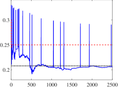
(2)

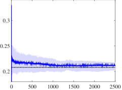
(3)

(4)

$\underset{\text{(kWh)}}{Q_{t}}$

(5)

(6)

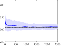
(7)

(8)

$\underset{\text{ (kWh${}^{2}$/\$)}}{\widehat{a}_{t}}$

(9)

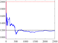
(10)

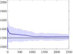
(11)

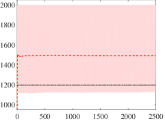
(12)

$\underset{\text{ (kWh)}}{\widehat{b}_{t}}$

(13)

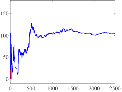
(14)

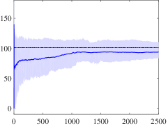
(15)

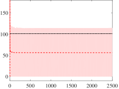
(16)

$\underset{\text{ (kWh)}}{\widehat{F}^{-1}_{t}(\alpha)}$

(17)

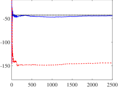
(18) (a) Sample paths.

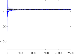
(19) (b) RPMP.

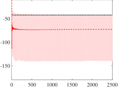
(20) (c) MP.

Figure 1: Figures in the first column include plots of sample paths generated by the randomly perturbed myopic policy (RPMP) ( [0.5ex]7mm1.25pt), the myopic policy (MP) ( [0.5ex]7mm1.25pt2.5pt), and the oracle optimal policy ([0.5ex]7mm1pt1pt). Figures in the second and third columns include mean/confidence-interval plots associated with sequences generated by the RPMP (second column) and the MP (third column), compared against their oracle optimal policy counterparts. The shaded area represents their middle 70% empirical confidence interval estimated using 100 independent experiments.

5.1 Discussion

The plots in Figure 1(c) illustrate an apparent lack of exploration in the sequence of posted prices generated by the myopic policy. That is to say, the myopic price sequence rapidly converges to a fixed value, which on average differs substantially from the oracle optimal price. The same is true for the sequence of forward contracts generated by the myopic policy. The premature convergence of the myopic price sequence, in turn, leads to incomplete learning with the parameter estimates converging incorrect values. As a consequence, the $T$-period regret incurred by the myopic policy grows linearly in $T$, as shown in Figure 2.

On the other hand, the persistent variation in the sequence of prices generated by the randomly perturbed myopic policy induces parameter estimates, which asymptotically converge to the true parameter values, which can be seen from the plots in Figure 1(b). In particular, notice that the (middle 70%) empirical confidence intervals associated with the posted price and contract sequences generated by the randomly perturbed myopic policy shrink to their respective optimal oracle values over time. This provides empirical evidence supporting our theoretical claim that the sequences of prices and contracts generated by the randomly perturbed myopic policy converge to their oracle optimal values in the mean square sense.

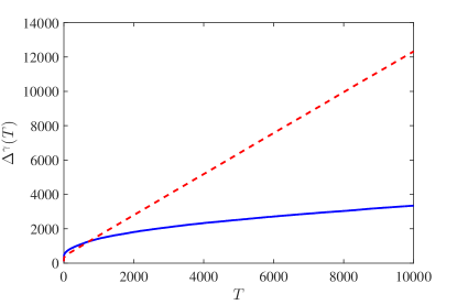
Figure 2: A plot of the $T$-period regret incurred by the randomly perturbed myopic policy ( [0.5ex]7mm1.25pt) compared to the $T$-period regret incurred by the myopic policy ( [0.5ex]7mm1.25pt2.3pt).

6 Conclusion

In this paper, we study the problem of co-optimizing an aggregator’s procurement and sale of demand response. The aggregator purchases energy in the form of demand reductions from a fixed group of residential customers, and sells the (a priori uncertain) aggregate demand reduction in a two-settlement wholesale electricity market. The customers’ aggregate demand function is assumed to be affine in price (with unknown parameters) and subject to unobservable, additive random shocks (with unknown distribution). We propose a data-driven policy—referred to as the randomly perturbed myopic policy—to guide the aggregator’s adaptation of its posted DR prices and forward contract offerings over time. We show that the proposed policy is consistent, meaning that the sequences of prices and contracts that it generates converge to the oracle optimal price and contract in the mean square sense. Moreover, we show that the regret incurred by the proposed policy over $T$ time periods is no more than $O(\log(T)\sqrt{T})$.

As a direction for future research, it would be interesting to generalize the techniques developed in this paper to accommodate time-varying and possibly nonlinear demand functions.

Appendix A Notation

Notation	Definition
$p_{t}$	DR price offered at time period $t$
$Q_{t}$	Forward contract commitment at time period $t$
$\pi_{t}$	DA energy price at time period $t$
$\pi^{+}_{t}$	RT overage price at time period $t$
$\pi^{-}_{t}$	RT shortage price at time period $t$
$\mu^{+}$	Expected value of the RT overage price at time period $t$
$\mu^{-}$	Expected value of the RT shortage price at time period $t$
$D_{t}$	Aggregate demand reduction at time period $t$
$\varepsilon_{t}$	Aggregate demand shock at time period $t$
$F(\cdot)$	Cumulative distribution function (CDF) of the aggregate
	demand shock $\varepsilon_{t}$ at each time period $t$
$\theta$	Demand model parameters $(a,b)$
$r_{t}(Q,p)$	Expected profit of the aggregator at time period $t$
$\Delta^{\gamma}(T)$	$T$-period regret incurred under feasible policy $\gamma$

Table 2: Table of notations.

Appendix B Proof of Lemma 1

Given a fixed pair $(Q,p)$, we have that

$$r_{t}(Q,p)= \pi_{t}Q-(ap^{2}+pb)+\mu^{+}\mathbb{E}\left[ap+b-Q+\varepsilon_{t}\right]^{+}$$

$$-\mu^{-}\mathbb{E}\left[Q-(ap+b)-\varepsilon_{t}\right]^{+}.$$

It is straightforward to show that $r_{t}(Q,p)$ is strictly concave in its arguments. It follows that one can characterize its unique maximizers as solutions to the first order optimality conditions:

$$\frac{\partial r_{t}(Q,p)}{\partial p} =-2ap-b+a\mu^{+}(1-F(Q-ap-b))+a\mu^{-}F(Q-ap-b)=0,$$ (20)

$$\frac{\partial r_{t}(Q,p)}{\partial Q} =\pi_{t}-\mu^{+}(1-F(Q-ap-b))-\mu^{-}F(Q-ap-b)=0.$$ (21)

The desired result follows.

Appendix C Proof of Lemma 2

Let $t\geq 1$, and fix $(Q_{t},p_{t})$. To streamline the proof, we define $Y_{t}:=Q_{t}-ap_{t}-b$ for each time period $t$. It follows that the expected profit of the aggregator can be expressed as

$$r_{t}(Q_{t},p_{t}) =\pi_{t}Y_{t}+\mathbb{E}\left[\mu^{+}[\varepsilon_{t}-Y_{t}]^{+}-\mu^{-}[Y_{t}-\varepsilon_{t}]^{+}\right]+(\pi_{t}-p_{t})(ap_{t}+b).$$

It will be helpful to decompose the expected profit as $r_{t}(Q_{t},p_{t})=r_{1t}(Q_{t},p_{t})+r_{2t}(Q_{t},p_{t})$, where

$$r_{1t}(Q_{t},p_{t}) :=\pi_{t}Y_{t}+\mathbb{E}\left[\mu^{+}[\varepsilon_{t}-Y_{t}]^{+}-\mu^{-}[Y_{t}-\varepsilon_{t}]^{+}\right],$$

$$r_{2t}(Q_{t},p_{t}) :=(\pi_{t}-p_{t})(ap_{t}+b).$$

It is straightforward to show that

$$r_{2t}(Q^{*}_{t},p^{*}_{t})-r_{2t}(Q_{t},p_{t})=a(p_{t}-p^{*}_{t})^{2}.$$ (22)

Now we show that for each time period $t$, we have

$$r_{1t}(Q^{*}_{t},p^{*}_{t})-r_{1t}(Q_{t},p_{t})\leq L(\mu^{-}-\mu^{+})(Y_{t}-Y^{*}_{t})^{2},$$ (23)

where $Y^{*}_{t}:=Q^{*}_{t}-ap^{*}_{t}-b$. It is straightforward to show that $Y^{*}_{t}=F^{-1}(\alpha_{t})$. Consider first the case in which $Y_{t}\geq Y^{*}_{t}$. It follows that

$$r_{1t}(Q^{*}_{t},p^{*}_{t})-r_{1t}(Q_{t},p_{t})$$

$$=\pi_{t}(Y^{*}_{t}-Y_{t})+\mu^{+}\int_{Y^{*}_{t}}^{\infty}(\varepsilon_{t}-Y^{*}_{t})\ dF-\mu^{+}\int_{Y_{t}}^{\infty}(\varepsilon_{t}-Y_{t})\ dF$$

$$\quad-\mu^{-}\int_{-\infty}^{Y^{*}_{t}}(Y^{*}_{t}-\varepsilon_{t})\ dF+\mu^{-}\int_{-\infty}^{Y_{t}}(Y_{t}-\varepsilon_{t})\ dF$$

$$=\pi_{t}(Y^{*}_{t}-Y_{t})+\mu^{+}\int_{Y^{*}_{t}}^{\infty}(Y_{t}-Y^{*}_{t})\ dF+\mu^{-}\int_{-\infty}^{Y^{*}_{t}}(Y_{t}-Y^{*}_{t})\ dF$$

$$\quad+(\mu^{-}-\mu^{+})\int_{Y^{*}_{t}}^{Y_{t}}(Y_{t}-\varepsilon_{t})\ dF$$

$$=(Y^{*}_{t}-Y_{t})\big{(}\pi_{t}-\mu^{+}(1-F(Y^{*}_{t}))-\mu^{-}F(Y^{*}_{t})\big{)}+(\mu^{-}-\mu^{+})\int_{Y^{*}_{t}}^{Y_{t}}(Y_{t}-\varepsilon_{t})\ dF$$

$$=(\mu^{-}-\mu^{+})\int_{Y^{*}_{t}}^{Y_{t}}(Y_{t}-\varepsilon_{t})\ dF,$$

where the last equality follows from the fact that $F(Y^{*}_{t})=F(F^{-1}(\alpha_{t}))=\alpha_{t}$. Now, using the fact that $F$ is bi-Lipschitz, we obtain

$$r_{1t}(Q^{*}_{t},p^{*}_{t})-r_{1t}(Q_{t},p_{t}) =(\mu^{-}-\mu^{+})\int_{Y^{*}_{t}}^{Y_{t}}(Y_{t}-\varepsilon_{t})\ dF$$

$$\leq(\mu^{-}-\mu^{+})(Y_{t}-Y^{*}_{t})\int_{Y_{t}^{*}}^{Y_{t}}\ dF$$

$$\leq L(\mu^{-}-\mu^{+})(Y_{t}-Y^{*}_{t})^{2}.$$

For the case in which $Y_{t}<Y^{*}_{t}$, one can obtain an identical upper bound using an analogous approach as above. Finally, combining Inequality (23) and Equation (22) with the fact that $Y_{t}-Y^{*}_{t}=Q_{t}-Q^{*}_{t}-a(p_{t}-p^{*}_{t})$ yields the desired upper bound on regret.

Appendix D Proof of Lemma 3

To simplify the presentation in the sequel, we define $u_{t}$ and $U_{t}$ as follows

$$u_{t}:=\sum_{k=1}^{t}\begin{bmatrix}p_{k}\\ 1\end{bmatrix}\varepsilon_{k}\quad\text{and}\quad U_{t}:=u_{t}^{\top}P_{t}^{-1}u_{t}.$$

Recall from Equation (10) that $\theta_{t}-\theta=P_{t}^{-1}u_{t}$. Then,

$$\mathbb{E}^{\gamma}\left[\|\widehat{\theta}_{t}-\theta\|^{2}\right] \leq\mathbb{E}^{\gamma}\left[\|P_{t}^{-1}u_{t}\|^{2}\right]\leq\mathbb{E}^{\gamma}\left[\|P_{t}^{-1/2}\|^{2}\|P_{t}^{-1/2}u_{t}\|^{2}\right],$$

where the last inequality follows from the Cauchy-Schwarz inequality. Using the definition of matrix norms, it holds that

$$\|P_{t}^{-1/2}\|^{2}=\left(\lambda_{\mathsf{max}}\left(P_{t}^{-1/2}\right)\right)^{2}=\lambda_{\mathsf{min}}(P_{t})^{-1},$$

where $\lambda_{\mathsf{max}}(A)$ and $\lambda_{\mathsf{min}}(A)$ are defined as the largest and smallest eigenvalues of the matrix $A$, respectively. We construct a lower bound on $\lambda_{\mathsf{min}}(P_{t})$ similar to [34, Lemma 1]. To bound $\lambda_{\mathsf{min}}(P_{t})$, we first find the characteristic polynomial of $P_{t}$. Recall the definition of $P_{t}$, that is

$$P_{t}=\sum_{k=1}^{t}\begin{bmatrix}p_{k}\\ 1\end{bmatrix}\begin{bmatrix}p_{k}\\ 1\end{bmatrix}^{\top}=\begin{bmatrix}\sum_{k=1}^{t}p_{k}^{2}&\sum_{k=1}^{t}p_{k}\\ \sum_{k=1}^{t}p_{k}&t\end{bmatrix}=\begin{bmatrix}\sum_{k=1}^{t}p_{k}^{2}&t\bar{p}_{t}\\ t\bar{p}_{t}&t\end{bmatrix}.$$

The characteristic polynomial of $P_{t}$ is given by

$$\lambda^{2}-\lambda\left(t+\sum_{k=1}^{t}p_{k}^{2}\right)+t^{2}V_{t}=0.$$ (24)

From Equation (24) it follows that

$$\lambda_{\mathsf{max}}(P_{t})+\lambda_{\mathsf{min}}(P_{t}) =t+\sum_{k=1}^{t}p_{k}^{2},$$ (25)

$$\lambda_{\mathsf{max}}(P_{t})\lambda_{\mathsf{min}}(P_{t}) =t^{2}V_{t}.$$ (26)

Define $\overline{p}$ as $\overline{p}:=\mu^{-}/2+\rho$, which upper bounds prices generated under the RPMP policy. From Equation 25 it follows that $\lambda_{\mathsf{max}}(P_{t})\leq(1+\overline{p}^{2})t$. Thus, using Equation 26, we get

$$\lambda_{\mathsf{min}}(P_{t})\geq\frac{tV_{t}}{1+\overline{p}^{2}}.$$

Using the lower bound on the minimum eigenvalue of $P_{t}$ and the definition of $U_{t}$, we get

$$\mathbb{E}^{\gamma}\left[\|\widehat{\theta}_{t}-\theta\|^{2}\right] \leq\mathbb{E}^{\gamma}\left[\lambda_{\mathsf{min}}(P_{t})^{-1}\|P_{t}^{-1/2}u_{t}\|^{2}\right]$$

$$\leq(1+\overline{p}^{2})\mathbb{E}^{\gamma}\left[\frac{U_{t}}{tV_{t}}\right].$$ (27)

Now we establish a result that lower bounds the price variance $V_{t}$ by a function of random variables $\xi_{1},\ldots,\xi_{t}$. Its proof is postponed to Appendix F.

Lemma 4 (Bound on $V_{t}$)

Under the randomly perturbed myopic policy (18) and (19), the price variance $V_{t}$ is lower bounded by

$$V_{t}\geq\frac{\Xi_{t}}{t}\quad\text{almost surely},$$ (28)

for $t\geq 3$. Here, $\Xi_{t}$ is defined as

$$\Xi_{t}:=\frac{1}{2}(p_{2}-p_{1})^{2}+\frac{2}{3}\rho^{2}\sum_{k=3}^{t}\xi_{k}.$$ (29)

By applying Inequality (28) to Inequality (27), we get

$$\mathbb{E}^{\gamma}\left[\|\widehat{\theta}_{t}-\theta\|^{2}\right]\leq(1+\overline{p}^{2})\mathbb{E}^{\gamma}\left[\frac{U_{t}}{\Xi_{t}}\right].$$ (30)

We now bound $\mathbb{E}^{\gamma}[U_{t}/\Xi_{t}]$ similar to Lai and Wei [39, Theorem 1]. They use the extended stochastic Liapounov functions and construct a recursive bound on $U_{t}$. Using a similar argument we construct a recursive bound on $\mathbb{E}^{\gamma}[U_{k}/\Xi_{t}]$ for $k=3,\ldots,t$. The proof of Lemma 5 is postponed to Appendix G.

Lemma 5

For all $t\geq 3$, it holds that

$$\mathbb{E}^{\gamma}\left[\frac{U_{t}}{\Xi_{t}}\right]\leq 2\sigma^{2}\mathbb{E}^{\gamma}\left[\frac{1}{\Xi_{t}}\right]+\sigma^{2}\sum_{k=3}^{t}\mathbb{E}^{\gamma}\left[\frac{1}{\Xi_{t}}\begin{bmatrix}p_{k}\\ 1\end{bmatrix}^{\top}P_{k}^{-1}\begin{bmatrix}p_{k}\\ 1\end{bmatrix}\right],$$ (31)

where $\sigma^{2}:=\mbox{Var}(\varepsilon_{t})\leq(\overline{\varepsilon}-\underline{\varepsilon})^{2}$.

Now we upper bound the second term in the right hand side of Inequality (31). It is straightforward to show that

$$\begin{bmatrix}p_{k}\\ 1\end{bmatrix}^{\top}P_{k}^{-1}\begin{bmatrix}p_{k}\\ 1\end{bmatrix} =\frac{1}{kV_{k}}\begin{bmatrix}p_{k}\\ 1\end{bmatrix}^{\top}\begin{bmatrix}1&-\bar{p}_{k}\\ -\bar{p}_{k}&V_{k}+\bar{p}_{k}^{2}\end{bmatrix}\begin{bmatrix}p_{k}\\ 1\end{bmatrix}=1-\frac{(k-1)V_{k-1}}{kV_{k}}+\frac{1}{k}.$$

Note that for all $x>0$, it holds that $1-x\leq\log(1/x)$. Thus,

$$\sum_{k=3}^{t}\begin{bmatrix}p_{k}\\ 1\end{bmatrix}^{\top}P_{k}^{-1}\begin{bmatrix}p_{k}\\ 1\end{bmatrix} \leq\sum_{k=3}^{t}\left(\log\left(\frac{kV_{k}}{(k-1)V_{k-1}}\right)+\frac{1}{k}\right)$$

$$=\log\left(\frac{tV_{t}}{2V_{2}}\right)+\sum_{k=3}^{t}\frac{1}{k}$$

$$\leq\log\left(\frac{tV_{t}}{2V_{2}}\right)+\log(t)$$

$$\leq\log\left(\frac{2\overline{p}^{2}}{(p_{2}-p_{1})^{2}}\right)+2\log(t)\quad\text{almost surely},$$ (32)

where the last inequality follows from the fact that $V_{t}\leq\overline{p}^{2}$ almost surely and $V_{2}=(1/4)(p_{2}-p_{1})^{2}$. By applying Inequality (32) and (31) to Inequality (30), we get

$$\mathbb{E}^{\gamma} \left[\|\widehat{\theta}_{t}-\theta\|^{2}\right]$$

$$\leq 2\sigma^{2}(1+\overline{p}^{2})\left(1+\log\left(\frac{\sqrt{2}\overline{p}}{|p_{2}-p_{1}|}\right)+\log(t)\right)\mathbb{E}^{\gamma}\left[\frac{1}{\Xi_{t}}\right]$$

$$\leq 2\sigma^{2}(1+\overline{p}^{2})\left(1+\frac{1}{\log(3)}\log\left(\frac{2\sqrt{2}\overline{p}}{|p_{2}-p_{1}|}\right)\right)\log(t)\mathbb{E}^{\gamma}\left[\frac{1}{\Xi_{t}}\right],$$ (33)

where the last inequality follows from the fact that $\log(t)+c\leq(1+c/\log(3))\log(t)$ for $t\geq 3$ and all $c\geq 0$, and the fact that $|p_{2}-p_{1}|\leq\overline{p}$. Finally, we establish an upper bound on $\mathbb{E}^{\gamma}[{1}/{\Xi_{t}}]$ in Lemma 6, which its proof is given in Appendix H.

Lemma 6

For $t\geq 3$, it holds that

$$\mathbb{E}^{\gamma}\left[\frac{1}{\Xi_{t}}\right]\leq\frac{3}{(p_{2}-p_{1})^{2}\eta t^{1-r}}.$$

Setting as follows yields the desired result.

$$K:=\frac{6\sigma^{2}(1+\overline{p}^{2})}{(p_{2}-p_{1})^{2}\eta}\left(1+\frac{1}{\log(3)}\log\left(\frac{2\sqrt{2}\overline{p}}{|p_{2}-p_{1}|}\right)\right).$$

Appendix E Proof of Theorem 1

We first establish a result that relates pricing and contracting errors under the RPMP to the parameter estimation error. Its proof is postponed to Appendix I.

Lemma 7

Under the randomly perturbed myopic policy (18) and (19), it holds that

$$\mathbb{E}^{\gamma}\left[(p_{t}-p^{*}_{t})^{2}\right]\leq k_{1}\mathbb{E}^{\gamma}\left[\|\widehat{\theta}_{t-1}-\theta\|^{2}\right]+k_{2}t^{-r},$$ (34)

and

$$\mathbb{E}^{\gamma}\left[(Q_{t}-Q^{*}_{t}-a(p_{t}-p^{*}_{t}))^{2}\right]$$ (35)

$$\qquad\leq k_{3}\mathbb{E}^{\gamma}\left[\|\widehat{\theta}_{t-1}-\theta\|^{2}\right]+k_{4}\frac{1}{t-1}+k_{5}\frac{1}{\sqrt{t-1}}+k_{6}t^{-r},$$ (36)

for all $t\geq 3$.

We combine Lemmas 2 and 7 to obtain

$$\Delta^{\gamma}(T)\leq k_{0}+(k_{1}+k_{3}L(\mu^{-}-\mu^{+}))\sum_{t=3}^{T}\mathbb{E}^{\gamma}\left[\|\widehat{\theta}_{t-1}-\theta\|_{1}^{2}\right]$$

$$+\sum_{t=3}^{T}(k_{2}+k_{6}L(\mu^{-}-\mu^{+}))t^{-r}+L(\mu^{-}-\mu^{+})\left(k_{4}\frac{1}{t-1}+k_{5}\frac{1}{\sqrt{t-1}}\right)$$

$$\leq k_{0}+(k_{1}+k_{3}L(\mu^{-}-\mu^{+}))\sum_{t=2}^{T}\mathbb{E}^{\gamma}\left[\|\widehat{\theta}_{t}-\theta\|_{1}^{2}\right]$$

$$+(k_{2}+k_{6}L(\mu^{-}-\mu^{+}))\sum_{t=3}^{T}t^{-r}+L(\mu^{-}-\mu^{+})\sum_{t=2}^{T}\left(k_{4}\frac{1}{t}+k_{5}\frac{1}{\sqrt{t}}\right),$$ (37)

where $k_{0}:=\sum_{t=1}^{2}a(p_{t}-p^{*}_{t})^{2}+L(\mu^{-}-\mu^{+})(Q_{t}-Q^{*}_{t}-a(p_{t}-p^{*})^{2})$. Now by applying the bound on the parameter estimation error in Lemma 3 to Inequality (37), we get

$$\Delta^{\gamma}(T)\leq k_{0}+(k_{1}+k_{3}L(\mu^{-}-\mu^{+}))K\sum_{t=2}^{T}\frac{\log(t)}{t^{1-r}}$$

$$+(k_{2}+k_{6}L(\mu^{-}-\mu^{+}))\sum_{t=3}^{T}t^{-r}+L(\mu^{-}-\mu^{+})\sum_{t=2}^{T}\left(k_{4}\frac{1}{t}+k_{5}\frac{1}{\sqrt{t}}\right)$$

$$\leq k_{0}+(k_{1}+k_{3}L(\mu^{-}-\mu^{+}))K\frac{\log(T)}{r}T^{r}+\frac{k_{2}+k_{6}L(\mu^{-}-\mu^{+})}{1-r}T^{1-r}$$

$$+L(\mu^{-}-\mu^{+})\left(k_{4}\log(T)+2k_{5}\sqrt{T}\right)$$

$$\leq C_{0}+C_{1}\log(T)+\left(\frac{C_{2}}{1-r}\right)T^{1-r}+\left(\frac{C_{2}}{r}\right)\log(T)T^{r}.$$

The second inequality follows from the fact that for $r\in(0,1)$, we have that

$$\sum_{t=2}^{T}\frac{\log(t)}{t^{1-r}}\leq\int_{1}^{T}\frac{\log(x)}{x^{1-r}}dx\leq\frac{1}{r}\log(T)T^{r},$$

and

$$\sum_{t=3}^{T}t^{-r}\leq\int_{2}^{T}x^{-r}dx\leq\frac{1}{1-r}T^{1-r},$$

and that

$$\sum_{t=2}^{T}\frac{1}{t}\leq\int_{1}^{T}\frac{1}{x}dx=\log(T).$$

We complete the proof by defining the constants $C_{0}$, $C_{1}$, and $C_{2}$ as follows.

$$C_{0} :=k_{0},$$

$$C_{1} :=L(\mu^{-}-\mu^{+})k_{4},$$

$$C_{2} :=2L(\mu^{-}-\mu^{+})k_{5}+\max\left\{k_{2}+k_{6}L(\mu^{-}-\mu^{+}),(k_{1}+k_{3}L(\mu^{-}-\mu^{+}))K\right\}.$$

Appendix F Proof of Lemma 4

It is straightforward to show that

$$\sum_{k=1}^{t}(p_{k}-\bar{p}_{t})^{2}=\sum_{k=2}^{t}\frac{k-1}{k}(p_{k}-\bar{p}_{k-1})^{2}.$$

Then for the RPMP, we get

$$tV_{t} =\sum_{k=2}^{t}\frac{k-1}{k}(p_{k}-\bar{p}_{k-1})^{2}$$

$$=\frac{1}{2}(p_{2}-p_{1})^{2}+\sum_{k=3}^{t}\frac{k-1}{k}(p_{k}-\bar{p}_{k-1})^{2}$$

$$=\frac{1}{2}(p_{2}-p_{1})^{2}+\sum_{k=3}^{t}\frac{k-1}{k}(\rho\xi_{k}+(\widehat{p}_{k}-\bar{p}_{k-1})(1-\xi_{k}))^{2}$$

$$=\frac{1}{2}(p_{2}-p_{1})^{2}+\sum_{k=3}^{t}\frac{k-1}{k}\rho^{2}\xi_{k}^{2}+\sum_{k=3}^{t}\frac{k-1}{k}(\widehat{p}_{k}-\bar{p}_{k-1})^{2}(1-\xi_{k})^{2},$$

where the last equality follows from the fact that $\xi_{k}(1-\xi_{k})=0$ for all $k\geq 3$. Thus, almost surely it holds that

$$tV_{t} \geq\frac{1}{2}(p_{2}-p_{1})^{2}+\sum_{k=3}^{t}\frac{k-1}{k}\rho^{2}\xi_{k}^{2}$$

$$\geq\frac{1}{2}(p_{2}-p_{1})^{2}+\frac{2}{3}\rho^{2}\sum_{k=3}^{t}\xi_{k}^{2}$$

$$=\frac{1}{2}(p_{2}-p_{1})^{2}+\frac{2}{3}\rho^{2}\sum_{k=3}^{t}\xi_{k},$$

where the last equality follows from the fact that $\xi_{k}$ only takes values in $\{0,1\}$.

Appendix G Proof of Lemma 5

Recall from the definition of $\Xi_{t}$ in Equation (29) that it is only a function of $\xi_{3},\ldots,\xi_{t}$. Thus $\varepsilon_{k}$ is independent of $\Xi_{t}$ for all $k=1,\ldots,t$. Then,

$$\mathbb{E}^{\gamma}\left[\frac{U_{k}}{\Xi_{t}}\right] =\mathbb{E}^{\gamma}\left[\frac{1}{\Xi_{t}}\left(u_{k-1}+\begin{bmatrix}p_{k}\\ 1\end{bmatrix}\varepsilon_{k}\right)^{\top}P_{k}^{-1}\left(u_{k-1}+\begin{bmatrix}p_{k}\\ 1\end{bmatrix}\varepsilon_{k}\right)\right]$$

$$=\mathbb{E}^{\gamma}\left[\frac{1}{\Xi_{t}}u_{k-1}^{\top}P_{k}^{-1}u_{k-1}\right]+2\mathbb{E}^{\gamma}\left[\frac{1}{\Xi_{t}}u_{k-1}^{\top}P_{k}^{-1}\begin{bmatrix}p_{k}\\ 1\end{bmatrix}\varepsilon_{k}\right]$$

$$\quad+\mathbb{E}^{\gamma}\left[\frac{1}{\Xi_{t}}\begin{bmatrix}p_{k}\\ 1\end{bmatrix}^{\top}P_{k}^{-1}\begin{bmatrix}p_{k}\\ 1\end{bmatrix}\varepsilon_{k}^{2}\right]$$

$$=\mathbb{E}^{\gamma}\left[\frac{1}{\Xi_{t}}u_{k-1}^{\top}P_{k}^{-1}u_{k-1}\right]$$

$$\quad+2\mathbb{E}^{\gamma}\left[\frac{1}{\Xi_{t}}u_{k-1}^{\top}P_{k}^{-1}\begin{bmatrix}p_{k}\\ 1\end{bmatrix}\mathbb{E}^{\gamma}\left[\varepsilon_{k}\ \Big{|}\ \Xi_{t},p_{1},\ldots,p_{k},\varepsilon_{1},\ldots,\varepsilon_{k-1}\right]\right]$$

$$\quad+\mathbb{E}^{\gamma}\left[\frac{1}{\Xi_{t}}\begin{bmatrix}p_{k}\\ 1\end{bmatrix}^{\top}P_{k}^{-1}\begin{bmatrix}p_{k}\\ 1\end{bmatrix}\mathbb{E}^{\gamma}\left[\varepsilon_{k}^{2}\ \Big{|}\ \Xi_{t},p_{1},\ldots,p_{k},\varepsilon_{1},\ldots,\varepsilon_{k-1}\right]\right]$$

$$=\mathbb{E}^{\gamma}\left[\frac{1}{\Xi_{t}}u_{k-1}^{\top}P_{k}^{-1}u_{k-1}\right]+\sigma^{2}\mathbb{E}^{\gamma}\left[\frac{1}{\Xi_{t}}\begin{bmatrix}p_{k}\\ 1\end{bmatrix}^{\top}P_{k}^{-1}\begin{bmatrix}p_{k}\\ 1\end{bmatrix}\right],$$ (38)

where the third equality is a direct application of the law of iterated expectations. The last equality follows from the fact that $\mathbb{E}^{\gamma}\left[\varepsilon_{k}|\Xi_{t},p_{1},\ldots,p_{k},\varepsilon_{1},\ldots,\varepsilon_{k-1}\right]=0$ and $\mathbb{E}^{\gamma}\left[\varepsilon_{k}^{2}|\Xi_{t},p_{1},\ldots,p_{k},\varepsilon_{1},\ldots,\varepsilon_{k-1}\right]=\mbox{Var}(\varepsilon_{k})=\sigma^{2}$. Using Sherman-Morrison formula we get

$$P_{k}^{-1} =\left(P_{k-1}+\begin{bmatrix}p_{k}\\ 1\end{bmatrix}\begin{bmatrix}p_{k}\\ 1\end{bmatrix}^{\top}\right)^{-1}=P_{k-1}^{-1}-\frac{P_{k-1}^{-1}\begin{bmatrix}p_{k}\\ 1\end{bmatrix}\begin{bmatrix}p_{k}\\ 1\end{bmatrix}^{\top}P_{k-1}^{-1}}{1+\begin{bmatrix}p_{k}\\ 1\end{bmatrix}^{\top}P_{k-1}^{-1}\begin{bmatrix}p_{k}\\ 1\end{bmatrix}}.$$

It follows that,

$$\mathbb{E}^{\gamma}\left[\frac{1}{\Xi_{t}}u_{k-1}^{\top}P_{k}^{-1}u_{k-1}\right] =\mathbb{E}^{\gamma}\left[\frac{U_{k-1}}{\Xi_{t}}\right]-\mathbb{E}^{\gamma}\left[\frac{1}{\Xi_{t}}\frac{\left(u_{k-1}P_{k-1}^{-1}\begin{bmatrix}p_{k}\\ 1\end{bmatrix}\right)^{2}}{1+\begin{bmatrix}p_{k}\\ 1\end{bmatrix}^{\top}P_{k-1}^{-1}\begin{bmatrix}p_{k}\\ 1\end{bmatrix}}\right]$$

$$\leq\mathbb{E}^{\gamma}\left[\frac{U_{k-1}}{\Xi_{t}}\right],$$

where the inequality follows from the fact that the random variable in the second expectation is non-negative almost surely. By applying the above inequality to Inequality (38), we get

$$\mathbb{E}^{\gamma}\left[\frac{U_{k}}{\Xi_{t}}\right]-\mathbb{E}^{\gamma}\left[\frac{U_{k-1}}{\Xi_{t}}\right]\leq\sigma^{2}\mathbb{E}^{\gamma}\left[\frac{1}{\Xi_{t}}\begin{bmatrix}p_{k}\\ 1\end{bmatrix}^{\top}P_{k}^{-1}\begin{bmatrix}p_{k}\\ 1\end{bmatrix}\right].$$

By summing the two sides of the above inequality, we get

$$\mathbb{E}^{\gamma}\left[\frac{U_{t}}{\Xi_{t}}\right]\leq\mathbb{E}\left[\frac{U_{2}}{\Xi_{t}}\right]+\sigma^{2}\sum_{k=3}^{t}\mathbb{E}^{\gamma}\left[\frac{1}{\Xi_{t}}\begin{bmatrix}p_{k}\\ 1\end{bmatrix}^{\top}P_{k}^{-1}\begin{bmatrix}p_{k}\\ 1\end{bmatrix}\right].$$

To compute the first term in the above inequality we compute $U_{2}$. Recall that $p_{1}$ and $p_{2}$ are deterministic constants. Then,

$$U_{2} =\frac{1}{(p_{2}-p_{1})^{2}}\begin{bmatrix}p_{1}\varepsilon_{1}+p_{2}\varepsilon_{2}\\ \varepsilon_{1}+\varepsilon_{2}\end{bmatrix}^{\top}\begin{bmatrix}2&-(p_{1}+p_{2})\\ -(p_{1}+p_{2})&p_{1}^{2}+p_{2}^{2}\end{bmatrix}\begin{bmatrix}p_{1}\varepsilon_{1}+p_{2}\varepsilon_{2}\\ \varepsilon_{1}+\varepsilon_{2}\end{bmatrix}$$

$$=\frac{1}{p_{2}-p_{1}}\begin{bmatrix}p_{1}\varepsilon_{1}+p_{2}\varepsilon_{2}\\ \varepsilon_{1}+\varepsilon_{2}\end{bmatrix}^{\top}\begin{bmatrix}-\varepsilon_{1}+\varepsilon_{2}\\ p_{2}\varepsilon_{1}-p_{1}\varepsilon_{2}\end{bmatrix}$$

$$=\varepsilon_{1}^{2}+\varepsilon_{2}^{2}.$$

The desired inequality follows from independence of $\varepsilon_{1}$ and $\varepsilon_{2}$ from $\Xi_{t}$.

Appendix H Proof of Lemma 6

Let $X_{k}\sim\mbox{Ber}(p_{k})$ and $Y_{k}\sim\mbox{Ber}(q_{k})$ be sequences of independent Bernoulli random variables such that $p_{k}\geq q_{k}$ for all $k=1,\ldots,t$. Then, for all $c>0$ and all $t\geq 1$ using the law of iterated expectations we get

$$\mathbb{E}\left[\frac{1}{c+\sum_{k=1}^{t}X_{k}}\right]$$

$$=(1-p_{t})\mathbb{E}\left[\frac{1}{c+\sum_{k=1}^{t-1}X_{k}}\right]+p_{t}\mathbb{E}\left[\frac{1}{c+1+\sum_{k=1}^{t-1}X_{k}}\right]$$

$$=\mathbb{E}^{\gamma}\left[\frac{1}{c+\sum_{k=1}^{t-1}X_{k}}\right]-p_{t}\mathbb{E}\left[\frac{1}{\left(c+\sum_{k=1}^{t-1}X_{k}\right)\left(1+c+\sum_{k=1}^{t-1}X_{k}\right)}\right]$$

Using the fact that $p_{t}\geq q_{t}$, we get

$$\mathbb{E}\left[\frac{1}{c+\sum_{k=1}^{t}X_{k}}\right]$$

$$\leq\mathbb{E}\left[\frac{1}{c+\sum_{k=1}^{t-1}X_{k}}\right]-q_{t}\mathbb{E}\left[\frac{1}{\left(c+\sum_{k=1}^{t-1}X_{k}\right)\left(1+c+\sum_{k=1}^{t-1}X_{k}\right)}\right]$$

$$=\mathbb{E}\left[\frac{1}{c+\sum_{k=1}^{t-1}X_{k}+Y_{t}}\right].$$

Using a similar argument, one can show that for all $\tau=1,\ldots,t$, it holds that

$$\mathbb{E}\left[\frac{1}{c+\sum_{k=1}^{\tau}X_{k}+\sum_{k=\tau+1}^{t}Y_{k}}\right]\leq\mathbb{E}\left[\frac{1}{c+\sum_{k=1}^{\tau-1}X_{k}+\sum_{k=\tau}^{t}Y_{k}}\right].$$

By taking the sum of the both sides of the above inequality from $\tau=1$ to $\tau=t$, we get

$$\mathbb{E}\left[\frac{1}{c+\sum_{k=1}^{t}X_{k}}\right]\leq\mathbb{E}\left[\frac{1}{c+\sum_{k=1}^{t}Y_{k}}\right].$$

Now let $q_{k}=q$ for all $k=1,\ldots,t$. It follows that in this case $\sum_{k=1}^{t}Y_{k}$ is a Binomial random variable with parameters $(t,q)$. Then

$$\mathbb{E}\left[\frac{1}{c+\sum_{k=1}^{t}Y_{k}}\right] =\sum_{k=0}^{t}\frac{1}{c+k}{t\choose k}q^{k}(1-q)^{t-k}$$

$$=\sum_{k=0}^{t}\frac{1+k}{c+k}\frac{1}{1+k}{t\choose k}q^{k}(1-q)^{t-k}$$

$$\leq\frac{1}{c}\sum_{k=0}^{t}\frac{1}{1+k}{t\choose k}q^{k}(1-q)^{t-k}$$

$$=\frac{1}{c(t+1)q}\sum_{k=0}^{t}{t+1\choose k+1}q^{k+1}(1-q)^{t-k}$$

$$=\frac{1}{c(t+1)q}\left(1-(1-q)^{t+1}\right).$$

Thus,

$$\mathbb{E}\left[\frac{1}{c+\sum_{k=1}^{t}Y_{k}}\right]\leq\frac{1}{c(t+1)q}.$$

It follows from the above that for all $t\geq 3$

$$\mathbb{E}\left[\frac{1}{c+\sum_{k=3}^{t}Y_{k}}\right]\leq\frac{1}{c(t-1)q}\leq\frac{3}{2ctq}.$$

Using the fact that $\eta k^{-r}\geq\eta t^{-r}$ for $k=3,\ldots,t$, and by setting $q=\eta t^{-r}$ we get

$$\mathbb{E}^{\gamma}\left[\frac{1}{\Xi_{t}}\right]=\frac{3}{2\rho^{2}}\mathbb{E}^{\gamma}\left[\frac{1}{3(p_{2}-p_{1})^{2}/(4\rho^{2})+\sum_{k=3}^{t}\xi_{k}}\right]\leq\frac{3}{(p_{2}-p_{1})^{2}\eta t^{1-r}}.$$

Appendix I Proof of Lemma 7

Using the fact that $\xi_{t}(1-\xi_{t})=0$ for all $t\geq 3$, we obtain

$$\mathbb{E}^{\gamma}\left[(p_{t}-p^{*}_{t})^{2}\right] =\mathbb{E}^{\gamma}\left[\left((\widehat{p}_{t}-p^{*}_{t})(1-\xi_{t})+(\bar{p}_{t-1}-p^{*}_{t}+\rho)\xi_{t}\right)^{2}\right]$$

$$=\mathbb{E}^{\gamma}\left[(\widehat{p}_{t}-p^{*}_{t})^{2}\right]\mathbb{E}\left[(1-\xi_{t})^{2}\right]+\mathbb{E}^{\gamma}\left[(\bar{p}_{t-1}-p^{*}_{t}+\rho)^{2}\right]\mathbb{E}\left[\xi_{t}^{2}\right]$$

$$=\mathbb{E}^{\gamma}\left[(\widehat{p}_{t}-p^{*}_{t})^{2}\right](1-\eta t^{-r})+\mathbb{E}^{\gamma}\left[(\bar{p}_{t-1}-p^{*}_{t}+\rho)^{2}\right]\eta t^{-r}$$

$$\leq\mathbb{E}^{\gamma}\left[(\widehat{p}_{t}-p^{*}_{t})^{2}\right]+\mathbb{E}^{\gamma}\left[(\bar{p}_{t-1}-p^{*}_{t}+\rho)^{2}\right]\eta t^{-r}.$$

The second equality follows from the fact that $\xi_{t}$ is independent from $\widehat{p}_{t}$ and $\bar{p}_{t-1}$. Using Equation (17), it is not difficult to show that

$$\widehat{p}_{t}-p^{*}_{t}=\frac{1}{2a\widehat{a}_{t}}\begin{bmatrix}b\\ -a\end{bmatrix}^{\top}(\widehat{\theta}_{t}-\theta).$$

Then,

$$|\widehat{p}_{t}-p^{*}_{t}|\leq\frac{\sqrt{a^{2}+b^{2}}}{2a\underline{a}}\|\widehat{\theta}_{t}-\theta\|.$$

Using the above inequality, and the fact that $|\bar{p}_{t-1}-p^{*}_{t}+\rho|\leq\overline{p}+\rho$ for all $t\geq 3$, we obtain

$$\mathbb{E}^{\gamma}\left[(p_{t}-p^{*}_{t})^{2}\right] \leq k_{1}\mathbb{E}^{\gamma}\left[\|\widehat{\theta}_{t-1}-\theta\|^{2}\right]+k_{2}t^{-r},$$

where

$$k_{1} :=\frac{a^{2}+b^{2}}{4a^{2}\underline{a}^{2}}\quad\text{and}\quad k_{2}:=(\overline{p}+\rho)^{2}\eta.$$

Under the randomly perturbed myopic policy for $t\geq 3$, using the law of total expectation we get

$$\mathbb{E}^{\gamma}\left[(Q_{t}-Q^{*}_{t}-a(p_{t}-p^{*}_{t}))^{2}\right]$$

$$=(1-\eta t^{-r})\mathbb{E}^{\gamma}\left[(\widehat{Q}_{t}-Q^{*}_{t}-a(\widehat{p}_{t}-p^{*}_{t}))^{2}\right]$$

$$\qquad+\eta t^{-r}\mathbb{E}^{\gamma}\left[(\widehat{Q}_{t}-Q^{*}_{t}-a(\bar{p}_{t-1}-p^{*}_{t}+\rho))^{2}\right]$$

$$\leq\mathbb{E}^{\gamma}\left[(\widehat{Q}_{t}-Q^{*}_{t}-a(\widehat{p}_{t}-p^{*}_{t}))^{2}\right]+k_{6}t^{-r},$$ (39)

where $k_{6}$ is defined as

$$k_{6}:=\eta\left(\frac{1}{2}(\mu^{-}\overline{a}+\overline{b}-b)+(\overline{\varepsilon}-\underline{\varepsilon})+a\overline{p}\right)^{2}.$$

For the first term in Inequality (39), using the fact that $\widehat{Q}_{t}=\widehat{a}_{t}\widehat{p}_{t}+\widehat{b}_{t}+\widehat{F}_{t}^{-1}(\alpha_{t})$ we get

$$\widehat{Q}_{t}-Q^{*}_{t}-a(\widehat{p}_{t}-p^{*}_{t}) =(\widehat{a}_{t-1}-a)\widehat{p}_{t}+(\widehat{b}_{t-1}-b)+\widehat{F}_{t-1}^{-1}(\alpha_{t})-F^{-1}(\alpha_{t})$$

$$=\begin{bmatrix}\widehat{p}_{t}\\ 1\end{bmatrix}^{\top}(\widehat{\theta}_{t-1}-\theta)+\widehat{F}_{t-1}^{-1}(\alpha_{t})-F^{-1}(\alpha_{t}),$$

Thus,

$$\mathbb{E}^{\gamma}\left[(\widehat{Q}_{t}-Q^{*}_{t}-a(\widehat{p}_{t}-p^{*}_{t}))^{2}\right]$$

$$=\mathbb{E}^{\gamma}\left[\left(\begin{bmatrix}\widehat{p}_{t}\\ 1\end{bmatrix}^{\top}(\widehat{\theta}_{t-1}-\theta)+\widehat{F}_{t-1}^{-1}(\alpha_{t})-F^{-1}(\alpha_{t})\right)^{2}\right]$$

$$\leq\mathbb{E}^{\gamma}\left[\left(2\sqrt{1+\overline{p}^{2}}\|\widehat{\theta}_{t-1}-\theta\|+|F_{t-1}^{-1}(\alpha_{t})-F^{-1}(\alpha_{t})|\right)^{2}\right].$$

The inequality follows from Inequality (14). Recall that $\widehat{\theta}_{t}$ is the TLSE. Thus, it holds that $\|\widehat{\theta}_{t}-\theta\|\leq\overline{\delta}$ surely, where $\overline{\delta}$ is defined as $\overline{\delta}:=\sqrt{(\overline{a}-\underline{a})^{2}+\overline{b}^{2}}$. Thus,

$$\mathbb{E}^{\gamma}\left[(\widehat{Q}_{t}-Q^{*}_{t}-a(\widehat{p}_{t}-p^{*}_{t}))^{2}\right]\leq 4(1+\overline{p}^{2})\mathbb{E}^{\gamma}\left[\|\widehat{\theta}_{t-1}-\theta\|_{1}^{2}\right]$$

$$\hskip 40.00006pt+\mathbb{E}\left[(F_{t-1}^{-1}(\alpha_{t})-F^{-1}(\alpha_{t}))^{2}\right]+4\overline{\delta}\sqrt{1+\overline{p}^{2}}\mathbb{E}\left[|F_{t-1}^{-1}(\alpha_{t})-F^{-1}(\alpha_{t})|\right].$$

To bound the second and the third terms in the right hand side of the above inequality, we use Inequality (15), and the fact that $|F_{t}^{-1}(\alpha_{t})-F^{-1}(\alpha_{t})|$ and $(F_{t}^{-1}(\alpha_{t})-F^{-1}(\alpha_{t}))^{2}$ are non-negative random variables. For $t\geq 2$, we have that

$$\mathbb{E}\left[\left|F_{t}^{-1}(\alpha_{t})-F^{-1}(\alpha_{t})\right|\right] =\int_{0}^{\infty}\mathbb{P}\left\{\left|F_{t}^{-1}(\alpha_{t})-F^{-1}(\alpha_{t})\right|\geq\delta\right\}d\delta$$

$$\leq\int_{0}^{\infty}2\exp\left(-\mu_{1}\delta^{2}t\right)d\delta$$

$$=\frac{\sqrt{\pi}}{\sqrt{\mu_{1}t}},$$ (40)

and

$$\mathbb{E}\left[\left(F_{t}^{-1}(\alpha_{t})-F^{-1}(\alpha_{t})\right)^{2}\right] =\int_{0}^{\infty}\mathbb{P}\left\{\left|F_{t}^{-1}(\alpha_{t})-F^{-1}(\alpha_{t})\right|\geq\sqrt{\delta}\right\}d\delta$$

$$\leq\int_{0}^{\infty}2\exp\left(-\mu_{1}\delta t\right)d\delta$$

$$=\frac{2}{\mu_{1}t}.$$ (41)

We conclude the proof by defining the constants $k_{3}$, $k_{4}$, and $k_{5}$ as

$$k_{3}:=4(1+\overline{p}^{2}),\quad k_{4}:=\frac{2}{\mu_{1}},\quad\text{and}\quad k_{5}:=4\overline{\delta}\frac{\sqrt{\pi(1+\overline{p}^{2})}}{\sqrt{\mu_{1}}}.$$

References

• [1] K. Khezeli, W. Lin, E. Bitar, Learning to buy (and sell) demand response, IFAC-PapersOnLine 50 (1) (2017) 6761 – 6767, 20th IFAC World Congress. doi:https://doi.org/10.1016/j.ifacol.2017.08.1193.
• [2] FERC, Order 719, Wholesale competition in regions with organized electric markets, Federal Energy Regulatory Commission.
• [3] E. Bitar, Y. Xu, Deadline differentiated pricing of deferrable electric loads, IEEE Transactions on Smart Grid 8 (1) (2017) 13–25.
• [4] H.-p. Chao, R. Wilson, Priority service: Pricing, investment, and market organization, The American Economic Review (1987) 899–916.
• [5] C. Chen, J. Wang, S. Kishore, A distributed direct load control approach for large-scale residential demand response, IEEE Transactions on Power Systems 29 (5) (2014) 2219–2228.
• [6] T. Ericson, Direct load control of residential water heaters, Energy Policy 37 (9) (2009) 3502–3512.
• [7] J. Iria, F. Soares, M. Matos, Optimal supply and demand bidding strategy for an aggregator of small prosumers, Applied Energydoi:https://doi.org/10.1016/j.apenergy.2017.09.002.
• [8] S. Kundu, N. Sinitsyn, S. Backhaus, I. Hiskens, Modeling and control of thermostatically controlled loads, arXiv preprint arXiv:1101.2157.
• [9] J. L. Mathieu, M. Kamgarpour, J. Lygeros, G. Andersson, D. S. Callaway, Arbitraging intraday wholesale energy market prices with aggregations of thermostatic loads, IEEE Transactions on Power Systems 30 (2) (2015) 763–772.
• [10] A. Nayyar, M. Negrete-Pincetic, K. Poolla, P. Varaiya, Duration-differentiated energy services with a continuum of loads, IEEE Transactions on Control of Network Systems 3 (2) (2016) 182–191.
• [11] G. Sharma, L. Xie, P. Kumar, Large population optimal demand response for thermostatically controlled inertial loads, in: Smart Grid Communications (SmartGridComm), 2013 IEEE International Conference on, IEEE, 2013, pp. 259–264.
• [12] C.-W. Tan, P. Varaiya, Interruptible electric power service contracts, Journal of Economic Dynamics and Control 17 (3) (1993) 495–517.
• [13] Y. Xu, N. Li, S. H. Low, Demand response with capacity constrained supply function bidding, IEEE Transactions on Power Systems 31 (2) (2016) 1377–1394.
• [14] S. Borenstein, M. Jaske, A. Ros, Dynamic pricing, advanced metering, and demand response in electricity markets, Journal of the American Chemical Society 128 (12) (2002) 4136–45.
• [15] L. Gan, U. Topcu, S. H. Low, Optimal decentralized protocol for electric vehicle charging, IEEE Transactions on Power Systems 28 (2) (2013) 940–951.
• [16] L. Jia, L. Tong, Q. Zhao, An online learning approach to dynamic pricing for demand response, arXiv preprint arXiv:1404.1325.
• [17] S. Li, W. Zhang, J. Lian, K. Kalsi, Market-based coordination of thermostatically controlled loads – part I: A mechanism design formulation, IEEE Transactions on Power Systems 31 (2) (2016) 1170–1178.
• [18] N. Li, L. Chen, S. H. Low, Optimal demand response based on utility maximization in power networks, in: Power and Energy Society General Meeting, 2011 IEEE, IEEE, 2011, pp. 1–8.
• [19] Z. Ma, D. S. Callaway, I. A. Hiskens, Decentralized charging control of large populations of plug-in electric vehicles, IEEE Transactions on Control Systems Technology 21 (1) (2013) 67–78.
• [20] P. Samadi, A.-H. Mohsenian-Rad, R. Schober, V. W. Wong, J. Jatskevich, Optimal real-time pricing algorithm based on utility maximization for smart grid, in: Smart Grid Communications (SmartGridComm), 2010 First IEEE International Conference on, IEEE, 2010, pp. 415–420.
• [21] P. Yang, G. Tang, A. Nehorai, A game-theoretic approach for optimal time-of-use electricity pricing, IEEE Transactions on Power Systems 28 (2) (2013) 884–892.
• [22] C. Campaigne, S. S. Oren, Firming renewable power with demand response: an end-to-end aggregator business model, Journal of Regulatory Economics (2015) 1–37.
• [23] H.-p. Chao, Competitive electricity markets with consumer subscription service in a smart grid, Journal of Regulatory Economics 41 (1) (2012) 155–180.
• [24] C. Crampes, T.-O. Léautier, Demand response in adjustment markets for electricity, Journal of Regulatory Economics 48 (2) (2015) 169–193.
• [25] J. Levin, L. Einav, C. Farronato, N. Sundaresan, Auctions versus posted prices in online markets, Journal of Political Economydoi:10.1086/695529.
• [26] H.-p. Chao, Demand response in wholesale electricity markets: the choice of customer baseline, Journal of Regulatory Economics 39 (1) (2011) 68–88.
• [27] C. Chelmis, M. R. Saeed, M. Frincu, V. Prasanna, Curtailment estimation methods for demand response: Lessons learned by comparing apples to oranges, in: Proceedings of the 2015 ACM Sixth International Conference on Future Energy Systems, ACM, 2015, pp. 217–218.
• [28] K. Coughlin, M. A. Piette, C. Goldman, S. Kiliccote, Statistical analysis of baseline load models for non-residential buildings, Energy and Buildings 41 (4) (2009) 374–381.
• [29] W. Ma, S. Fang, G. Liu, R. Zhou, Modeling of district load forecasting for distributed energy system, Applied Energy 204 (2017) 181–205.
• [30] A. Dvoretzky, J. Kiefer, J. Wolfowitz, Asymptotic minimax character of the sample distribution function and of the classical multinomial estimator, The Annals of Mathematical Statistics (1956) 642–669.
• [31] V. Borkar, P. Varaiya, Identification and adaptive control of markov chains, SIAM Journal on Control and Optimization 20 (4) (1982) 470–489.
• [32] P. R. Kumar, P. Varaiya, Stochastic systems: Estimation, identification, and adaptive control, SIAM, 2015.
• [33] T. Lai, H. Robbins, Iterated least squares in multiperiod control, Advances in Applied Mathematics 3 (1) (1982) 50–73.
• [34] A. V. den Boer, B. Zwart, Simultaneously learning and optimizing using controlled variance pricing, Management science 60 (3) (2013) 770–783.
• [35] N. B. Keskin, A. Zeevi, Dynamic pricing with an unknown demand model: Asymptotically optimal semi-myopic policies, Operations Research 62 (5) (2014) 1142–1167.
• [36] B. Chen, X. Chao, H.-S. Ahn, Coordinating pricing and inventory replenishment with nonparametric demand learning, Available at SSRN 2694633.
• [37] DoE, Benefits of demand response in electricity markets and recommendations for achieving them, US Dept. Energy, Washington, DC, USA, Tech. Rep.
• [38] A. Faruqui, S. Sergici, Household response to dynamic pricing of electricity: a survey of 15 experiments, Journal of Regulatory Economics 38 (2) (2010) 193–225.
• [39] T. L. Lai, C. Z. Wei, Least squares estimates in stochastic regression models with applications to identification and control of dynamic systems, The Annals of Statistics (1982) 154–166.