Optimal Trade Execution Under Endogenous Pressure to Liquidate: Theory and Numerical Solutions

Abstract

We study optimal liquidation of a trading position (so-called block order or meta-order) in a market with a linear temporary price impact (Kyle, 1985). We endogenize the pressure to liquidate by introducing a downward drift in the unaffected asset price while simultaneously ruling out short sales. In this setting the liquidation time horizon becomes a stopping time determined endogenously, as part of the optimal strategy. We find that the optimal liquidation strategy is consistent with the square-root law which states that the average price impact per share is proportional to the square root of the size of the meta-order (Bershova and Rakhlin, 2013; Farmer et al., 2013; Donier et al., 2015; Tóth et al., 2016).

Mathematically, the Hamilton-Jacobi-Bellman equation of our optimization leads to a severely singular and numerically unstable ordinary differential equation initial value problem. We provide careful analysis of related singular mixed boundary value problems and devise a numerically stable computation strategy by re-introducing time dimension into an otherwise time-homogeneous task.

1 Introduction

We study optimal liquidation of an infinitely divisible asset when the execution price is subject to adverse price impact in proportion to the amount of the asset sold per unit of time, in line with Kyle (1985). The optimal liquidation strategy trades off expediency against the adverse price impact caused by a precipitous sale. However, our focus on liquidation is not fundamental; mutatis mutandis one can replace optimal liquidation with optimal acquisition in what follows. The novelty in our approach is that we rule out short sales in a falling market. This seemingly small change has a profound impact on the economics and mathematics of the problem. How and why this happens is the subject of the ensuing analysis.

Modelling of optimal execution with market impact is relatively new in the literature, going back to Almgren and Chriss (2000), Bertsimas and Lo (1998) and Subramanian and Jarrow (2001). Classical models Almgren and Chriss (2000), Bertsimas and Lo (1998), envisage a world where the unaffected price of the asset is a martingale and hence there is no pressure to trade quickly for an agent with linear utility. In these circumstances the incentive to trade is given by fiat – it is assumed that there is a fixed time limit by which the entire position must be liquidated.

The literature finds that optimal liquidation gives rise to ‘implementation shortfall’ (Perold, 1988) defined as the gap between the initial market value of the inventory and the expected revenue of the liquidation strategy; the latter always being lower due to the price impact. The shortfall itself is formed of two components, one due to ‘permanent price impact’ and another caused by ‘temporary impact’. The former cannot be influenced by the trading strategy, while the latter determines the optimal strategy and can be made arbitrarily small by making the liquidation time horizon longer. In this sense having more time is unambiguously beneficial to the trader.

A second strand of literature, Brown et al. (2010), Chen et al. (2014), Chen et al. (2015), identifies the motive to liquidate with a change in market conditions whereby tighter margin requirements lead to lower permitted amount of leverage. The change in market conditions occurs at discrete time points, while the optimal liquidation (deleveraging) is implemented continuously in time. Here for reasons of tractability the unaffected price is assumed constant during liquidation, although one could in principle use the results from the first strand of literature to make the modelling of the deleveraging phase more realistic.

In this paper we focus on the liquidation phase. Specifically, we study a situation where the unaffected price may be falling on average, which is highly plausible in a market with contracting liquidity. One expects that with the asset price decreasing the implementation shortfall should be more severe than in the martingale case. Surprisingly, the current literature finds that far from exhibiting a shortfall the optimal liquidation strategy may in this case record an expected surplus, see Schied (2013). On closer inspection one observes that the surplus arises due to short sale of the asset with subsequent acquisition at deflated price near the end of the allotted time horizon.

While strategic short sales in a bear market are not entirely implausible we feel it is important to examine a situation where such short sales are ruled out. The simplest way to achieve this is to stop the trading once the entire position has been liquidated. In doing so we recover the classical outcome from the martingale case whereby the price impact invariably leads to implementation shortfall. However, in a falling market without short sales it is no longer true that the shortfall can be made arbitrarily small by extending the liquidation time horizon.

Introduction of a stopping time is a novel feature in the optimal liquidation literature with a perfectly divisible asset. Previously, optimal stopping has appeared only in the context of optimal liquidation of an indivisible asset, see Mamer (1986) and Henderson and Hobson (2013). Although stopping on liquidation automatically precludes short sales, it does leave open the possibility of further intermediate acquisition. Ex-post it turns out that intermediate acquisition is not optimal, see Proposition 7.1 and Theorem 7.2. We show that the presence of the stopping time dramatically changes mathematical properties of the Hamilton-Jacobi-Bellman equation and leads to a severely singular and numerically unstable initial value problem. Part of our research contribution is in providing a comprehensive theoretical and numerical analysis of this HJB equation and related singular boundary value problems.

The paper is organized as follows. In Section 2 we survey related literature and present our model. In Section 3 we discuss reduction of our HJB partial differential equation (PDE) to an ordinary differential equation (ODE). Section 4 offers a probabilistic and control-theoretic interpretation of this reduction. Section 5 describes the singularity of the initial value problem (IVP) for the ODE of Section 3, while Section 6 shows how to obtain uniqueness from a related boundary value problem (BVP). In Section 7 we characterize the optimal strategy and its value function by means of the BVP of Section 6. In Section 8 we introduce and theoretically analyze a related PDE BVP which leads to a stable numerical scheme and present numerical results. Section 9 concludes.

2 Our model and related literature

We take the point of view of a trader with inventory $Z$ whose initial value $Z(0)>0$ is given. The modelling is based on the premise that there is some price process $S$ – often called the ‘unaffected price’ – with exogenously given dynamics that governs the evolution of the asset price in the absence of our trading. In our case the unaffected price $S$ is a geometric Brownian motion

$$dS(t)=\lambda S(t)dt+\sigma S(t)dB(t),$$ (2.1)

where $B$ is a Brownian motion in its natural filtration.

The inventory attracts interest rate $r,$ which becomes a storage cost when $r<0$. We assume that the inventory is sold off continuously at a (stochastic) rate $v:=-dZ/dt$ so that $v$ represents the amount of inventory sold per unit of time. Consequently, the inventory dynamics read

$$dZ(t)=\left(rZ(t)-v(t)\right)dt.$$ (2.2)

Let $T(Z=0)$ be the first time when the entire inventory is disposed of. For a given pair of initial values

$$s=S(0),z=Z(0),$$ (2.3)

the expected discounted revenue from the disposal of the asset is given by

$$J(s,z,v)=E_{s,z}\left[\int_{0}^{T(Z=0)}e^{-\rho t}(S(t)-\eta v(t))v(t)dt\right],$$ (2.4)

where $S-\eta v$ is the ‘affected price’ of the asset. In our setting $\eta$ measures the strength of ‘temporary impact’ the selling speed $v$ has on the price. The discount factor $\rho$ captures the opportunity cost of not holding alternative assets. The entire model is based on Černý (1999).

The task is to find optimal liquidation strategy $v$ that maximizes

$$V(s,z):=\sup_{v\in\mathcal{A}}J(s,z,v).$$ (2.5)

We say that $v$ is an admissible control, and write $v\in\mathcal{A}$, if process $v$ is predictable,

$$E\left[\int_{0}^{t}\left|v(s)\right|^{m}ds\right]<\infty\text{ for all }t>0\text{ and }m=1,2,\ldots,$$ (2.6)

and

$$E\left(\int_{0}^{T(Z=0)}e^{-\rho s}\left|v(t)(S(t)-\eta v(t))\right|dt\right)<\infty.$$ (2.7)

The optimization in our model can be seen, for specific parameter choices, as a special case of Ankirchner and Kruse (2013), Forsyth et al. (2012) and Schied (2013), with the crucial difference that in our case the liquidation time horizon is endogenous. We make a standing assumption that the time discounting is stronger than the expected appreciation and the interest on the asset combined,

$$\rho>\lambda+r.$$ (2.8)

To conclude this section we wish to make several observations that justify the choice of our modelling framework. The extant literature contains a number of variations on the model presented above. The trading may be discrete, rather than continuous, the unaffected price $S$ may be specified differently and the optimization criterion may involve a utility function. In common, existing models assume $T$ is fixed and exogenously given.

The most commonly considered specification for the affected price reads

$$\tilde{S}:=S-\gamma(Z(0)-Z_{-}-\frac{1}{2}\Delta Z)-\eta_{1}v+\eta_{2}\Delta Z,\text{ }$$ (2.9)

where $\gamma(Z(0)-Z_{-}-\frac{1}{2}\Delta Z)$ is the ‘permanent’ price impact while $\eta_{1}v$ and $\eta_{2}\Delta Z,$ respectively, are known as ‘temporary’ price impacts in the continuous-time and discrete-time literature, respectively. It is assumed either that there is a finite number of fixed dates $\{t_{i}\}_{i=1}^{N}$ where $Z$ is allowed to jump (discrete-time models) or that $Z$ changes continuously at a stochastic time rate $-v$ (continuous-time models). In each case $Z$ is taken to be a predictable semimartingale with left limit process $Z_{-}$ and jumps $\Delta Z=Z-Z_{-}$. Models in this category include Ankirchner et al. (2016), Brown et al. (2010), Chen et al. (2014), Gatheral and Schied (2011), Schied (2013), Schied and Schöneborn (2009) Ting et al. (2007) in continuous time and Almgren and Chriss (2000), Bertsimas and Lo (1998) in discrete time. Other impact specifications can be found, for example, in Chen et al. (2015), Cheridito and Sepin (2014), Forsyth (2011), Lorenz and Almgren (2011), Subramanian and Jarrow (2001) and Ting et al. (2007).

The revenue $R(T)$ from liquidation over a fixed time horizon $T$ is given by $R(T):=\int_{0}^{T}-\tilde{S}(t)dZ(t)$. When the unaffected asset price process $S$ is a martingale, integration by parts together with suitable boundedness of $Z$ and boundary condition $Z(T)=0$ yields

$$E[R(T)]=Z(0)S(0)-\frac{\gamma}{2}Z(0)^{2}-\eta_{1}\int_{0}^{T}v^{2}(t)dt-\eta_{2}\sum_{i=1}^{N}\left(\Delta Z(t_{i}\right)^{2}.$$

This equality offers several important insights:

1. Permanent impact (as defined here) has no strategic influence and in the absence of temporary impact ($\eta_{1}=\eta_{2}=0$) any strategy $Z$ is optimal. The expected implementation shortfall $Z(0)S(0)-E[R(T)]=\frac{\gamma}{2}Z(0)^{2}$ is strictly positive.

2. With temporary impact it is optimal to liquidate at a constant rate, regardless of the strength of the permanent impact. The additional implementation shortfall equals $\eta_{1}Z(0)^{2}/T$ in continuous time and $\eta_{2}Z(0)^{2}/N$ in discrete time, respectively.

These observations suggest that temporary impact is responsible for the majority of strategic interaction also in the drifting market and we conjecture that the optimal strategy will therefore not change dramatically when the permanent impact is included. This is not to say that the implementation shortfall would be unaffected by the presence of permanent impact. Given the complexity of analysis to follow and the likely marginal gains to our understanding from the presence of permanent impact on the optimal trading strategy we feel justified in leaving out the permanent impact from our analysis.

More recent studies, excellently summarized in Gatheral (2010), consider an intermediate form of impact where the execution price is given by the formula

$$S_{t}-\int_{0}^{t}f(v_{u})G(t-u)du.$$

Kernel $G$ is called the resiliency of the market and the two extreme cases, permanent impact and temporary impact, correspond to $G$ being constant or $G$ being the Dirac delta function, respectively. In Gatheral (2010) a case is made for a combination of power impact function, $f(v)=v^{\delta}$, with power law resiliency $G(x)=x^{-\gamma}$, $\delta+\gamma\geq 1$, the latter tending to a Dirac delta function as $\gamma\searrow 0$. We note that our setup corresponds to the limiting case $\delta=1,\gamma=0$ and we leave the analysis of the general impact function $f$ with general resiliency $G$ in the setup of this paper to future research.

3 HJB equation and dimension reduction

The value function $V$ defined in (2.5) formally solves the Hamilton-Jacobi-Bellman partial differential equation

$$\sup_{v}\{\frac{1}{2}s^{2}\sigma^{2}V_{ss}+\lambda sV_{s}+(rz-v)V_{z}-\rho V+v(s-\eta v)\}=0,\ s>0,z>0,$$

with formal optimal control

$$v^{\ast}=\frac{s-V_{z}}{2\eta},$$

giving rise to a quasilinear second order PDE

$$\frac{1}{2}s^{2}\sigma^{2}V_{ss}+\lambda sV_{s}+rzV_{z}-\rho V+\frac{(s-V_{z})^{2}}{4\eta}=0,$$ (3.1)

with an initial condition

$$V(s,0)=0.$$ (3.2)

The self-similarity

$$V(s,z)=s^{2}u(x)/(\eta\sigma^{2}),\ x=\eta\sigma^{2}z/s,$$ (3.3)

reduces (3.1, 3.2) to an initial value problem (IVP) for an ordinary differential equation (ODE)

$$x^{2}u^{\prime\prime} =axu^{\prime}+bu-(u^{\prime}-1)^{2}/2,\ x>0,$$ (3.4)

$$u(0) =0,$$ (3.5)

where

$$a:=2(\lambda-r+\sigma^{2})/\sigma^{2},\ b:=-2(2\lambda-\rho+\sigma^{2})/\sigma^{2}.$$ (3.6)

The self-similarity reduces a problem with 7 independent parameters $\rho,\lambda,r,\sigma,\eta,s\equiv S(0)$ and $z\equiv Z(0)$ to a problem with just three parameters: $a,$ $b$ and $x:=\eta\sigma^{2}z/s$.

4 Probabilistic interpretation of self-similarity

We begin by restating the HJB equation (3.1) in its variational form,

$$\sup_{v(0)}\left\{\text{drift}_{0}\left(e^{-\rho t}V(S,Z)\right)+v(0)\left(S(0)-\eta v(0)\right)\right\}=0.$$

Plug in the self-similarity form of the value function $V(S,Z)=S^{2}u\left(\eta\sigma^{2}Z/S\right)/(\eta\sigma^{2})$ and rearrange to obtain

$$\sup_{v(0)}\left\{\text{drift}_{0}\left(e^{-\rho t}\frac{S^{2}}{S(0)^{2}}u\left(\frac{\eta\sigma^{2}Z}{S}\right)\right)+\eta\sigma^{2}\frac{v(0)}{S(0)}\left(1-\eta\frac{v(0)}{S(0)}\right)\right\}=0.$$

The next steps involve i) changing measure to $\hat{P}$ given by $\frac{d\hat{P}_{t}}{dP_{t}}=\frac{S(t)^{2}}{S(0)^{2}}e^{-\left(2\lambda+\sigma^{2}\right)t}$ where $\hat{P}_{t}$ and $P_{t}$ are restrictions of $\hat{P}$ and $P$ to $\mathcal{F}_{t}$; ii) defining a new state variable $X:=\eta\sigma^{2}Z/S$; and iii) reparametrizing the control to $g:=\eta v/S,$ which yields

$$\sup_{g(0)}\left\{\widehat{\text{drift}}_{0}\left(e^{(2\lambda+\sigma^{2}-\rho)t}u\left(X\right)\right)+\sigma^{2}g(0)\left(1-g(0)\right)\right\}=0.$$ (4.1)

The Itō formula for $X$ reads

$$dX=\left(rX-\sigma^{2}g\right)dt+X\left(-\frac{dS}{S}+\frac{d[S,S]}{S^{2}}\right),$$

while from the Girsanov theorem we obtain $\widehat{\text{drift}}\left(\mathcal{L}(S)\right)=\lambda+2\sigma^{2}$, which implies

$$dX=\left((r-\lambda-\sigma^{2})X-\sigma^{2}g\right)dt+\sigma^{2}Xd\hat{B},$$ (4.2)

where $\hat{B}:=-\mathcal{L}(S)+(\lambda+2\sigma^{2})t$ is a Brownian motion under $\hat{P}$ and $\mathcal{L}(S)$ denotes the stochastic logarithm of $S,$ $d\mathcal{L}(S)=dS/S$. In the final step we perform a time change from $t$ to $\sigma^{2}t,$ defining $\hat{X}(t):=X(t/\sigma^{2})$ and $\hat{W}(t):=\sigma^{2}\hat{B}(t/\sigma^{2})$. This yields the dynamics

$$d\hat{X}=\left(\frac{r-\lambda-\sigma^{2}}{\sigma^{2}}\hat{X}-g\right)dt+\hat{X}d\hat{W},$$ (4.3)

while (4.1) changes to

$$\sup_{g(0)}\left\{\widehat{\text{drift}}_{0}\left(\exp\left(\frac{2\lambda+\sigma^{2}-\rho}{\sigma^{2}}t\right)u(\hat{X})\right)+g(0)\left(1-g(0)\right)\right\}=0.$$ (4.4)

With (4.3) in hand the optimality condition (4.4) explicitly reads

$$0 = \frac{1}{2}x^{2}u^{\prime\prime}(x)+\frac{r-\lambda-\sigma^{2}}{\sigma^{2}}xu^{\prime}(x)$$

$$+\frac{2\lambda+\sigma^{2}-\rho}{\sigma^{2}}u(x)+\frac{1}{4}\left(1-u^{\prime}(x)\right)^{2},$$

and the (formal) optimal control equals $g=(1-u^{\prime}(\hat{X}))/2$. It is furthermore clear that (4.4) itself is a HJB equation of an optimal control problem

$$u(x)=\sup_{g}\widehat{E}_{x=\hat{X}(0)}\left[\int_{0}^{T(\hat{X}=0)}\exp\left(-\frac{\rho-2\lambda-\sigma^{2}}{\sigma^{2}}t\right)g(t)(1-g(t))dt\right],$$ (4.5)

with $\hat{P}$-dynamics of $\hat{X}$ given by (4.3).

Note that the time in the transformed problem (4.5) is measured in terms of cumulative variance of the log return of the unaffected price, that is in ‘variance years’. One variance year corresponds to the physical time $t$ it takes to make $\sigma^{2}t=1$. With $\sigma=0.2$ one variance year is therefore equal to 25 calendar years. The new state variable $\hat{X}=\eta\sigma^{2}Z/S$ corresponds to the size of temporary price impact as a percentage of current price, assuming inventory $Z$ is completely liquidated at a constant rate over one variance year.

5 Singular initial value problem IVP₀

Hereafter we refer to the IVP (3.4, 3.5) as $\mathrm{IVP}_{0}$. Note $a+b>0$ if and only if our standing assumption (2.8) $\rho>r+\lambda$ holds. It has been shown in Brunovský et al. (2013) that $\mathrm{IVP}_{0}$ is highly degenerate at $0.$ For $a+b>0$ $\mathrm{IVP}_{0}$ has infinitely many solutions with identical asymptotics near $0$ given by the formal power series

$$h_{n}(x)=x-\frac{2}{3}\sqrt{2(a+b)}x^{3/2}+\sum_{i=2}^{n}k_{i}x^{1+i/2},\text{ }n\in\mathbb{N},$$ (5.1)

where $k_{i}$ are obtained recursively from

$$k_{n+1} = \frac{1}{3\left(n+3\right)k_{1}}\bigg{[}k_{n}\left(\left(n+2\right)(2a-n)+4b\right)$$

$$-\frac{1}{2}\sum_{j=1}^{n-1}(3+j)(n-j+3)k_{j+1}k_{n-j+1}\bigg{]}.$$

The series itself has zero radius of convergence for

$$6a+4b-3=:K_{1}>0>K_{2}:=6a+2b-9,$$

see (Quittner, 2015, Remark 2). Asymptotic expansion of derivatives of $u(x)$ is obtained by formal differentiation of the series in (5.1), ibid Theorem 1. Whenever $K_{1}=0$ or $K_{2}=0$ the power series ends at the 3rd element and constitutes a genuine solution of $\mathrm{IVP}_{0}$. This solution, however, is just one from a continuum and does not represent the optimal value function.

The highly degenerate nature of $\mathrm{IVP}_{0}$ does not stem from the singularity of the linear terms in the ODE, which is well known and rather innocuous in the context of the Black-Scholes model, but from the singularity of the non-linear term. Liang (2009) studies singular IVPs of the form $u^{\prime\prime}=x^{-1}f(x,u,u^{\prime})$ where $f$ is continuous. Note that the linear part of our ODE, $ax^{-1}u^{\prime},$ belongs to Liang’s category, but the non-linear term $x^{-2}\left(u^{\prime}-1\right)^{2}/2$ does not.

Liang, too, observes multiplicity of solutions, but this multiplicity is less pronounced than in our case. In Liang’s work $u(0)$ and $u^{\prime}(0)$ uniquely determine the first $\left\lceil\gamma\right\rceil$ derivatives of the solution, where $\gamma:=\frac{\partial}{\partial u^{\prime}}f(0,u(0),u^{\prime}(0))>0$, and, for non-integer $\gamma$, the solution becomes unique once the coefficient by $x^{\gamma}$ has been specified. Therefore, in Liang’s case all solutions differ asymptotically by a multiple of $x^{\gamma}$ near $0$.

In contrast, $\mathrm{IVP}_{0}$ has a continuum of solutions that differ asymptotically by

$$x^{\alpha}\exp\left(-\beta/\sqrt{x}\right),$$

where

$$\alpha:=2-\frac{2}{3}b,\qquad\beta:=\sqrt{8(a+b)},$$

see (Quittner, 2015, Theorems 2-5). These solutions invariably share their power series asymptotics to an arbitrary order as $x\searrow 0$. A uniqueness result relevant for the current paper can be summarized as follows:

Proposition 5.1.

Under the assumption $a+b>0$ there is a unique solution of $\mathrm{IVP}_{0}$ denoted by $u_{\infty}$ satisfying $u_{\infty}\in\mathcal{C}^{0}[0,\infty)\times\mathcal{C}^{2}(0,\infty)$,

$$0\leq u_{\infty}(x)\leq x\text{ for }x>0.$$ (5.2)

The solution $u_{\infty}$ further satisfies $u_{\infty}^{\prime}(0)=1,u_{\infty}^{\prime}(x)>0,u_{\infty}^{\prime\prime}(x)<0,u_{\infty}^{\prime\prime\prime}(x)>0$ for all $x>0$ as well as $u_{\infty}^{\prime}(x)\searrow 0$ for $x\rightarrow\infty$.

Proof.

See Proposition 5.1 in Brunovský et al. (2013).    

Proposition 5.2 reveals certain qualitative characteristics of solutions of $\mathrm{IVP}_{0}$ which can be observed empirically whenever an unstable numerical scheme is employed.

Proposition 5.2.

Any solution of (3.4) on $(\alpha,\beta)$ with $0\leq\alpha<\beta\leq\infty$ falls into one and only one of the following categories:

i) $u$ is constant;

ii) $u$ is strictly concave on $(\alpha,\beta)$;

iii) $u$ is strictly convex on $(\alpha,\beta)$;

iv) there is $x_{0}\in(\alpha,\beta)$ such that $u$ is strictly concave on $(\alpha,x_{0})$, strictly convex on $(x_{0},\beta)$ and $u^{\prime}(x)\geq u^{\prime}(x_{0})>0$ for all $x\in\left(\alpha,\beta\right)$;

v) there is $x_{0}\in(\alpha,\beta)$ such that $u$ is strictly convex on $(\alpha,x_{0})$, strictly concave on $(x_{0},\beta)$ and $u^{\prime}(x)\leq u^{\prime}(x_{0})<0$ for all $x\in\left(\alpha,\beta\right)$.

Proof.

The conclusions follow readily from Brunovský et al. (2013), Lemma 4.1, applied to the equation

$$x^{2}y^{\prime\prime}=(1+(a-2)x-y))y^{\prime}+\left(a+b\right)y,$$ (5.3)

with $y=u^{\prime}$, obtained by differentiation and re-arrangement of (3.4).    

6 Boundary value problem BVP_[0,∞)

In the context of the present paper it turns out to be advantageous to view Proposition 5.1 as a solution to a certain boundary value problem (BVP). We write $u^{\prime}(\infty):=\lim_{x\rightarrow\infty}u^{\prime}(x)$ whenever the limit on the right-hand side exists and complement the Dirichlet-type boundary condition $u(0)=0$ with a Neumann-type boundary condition

$$u^{\prime}\left(\infty\right)=0.$$ (6.1)

Hereafter we refer to the mixed boundary value problem (3.4, 3.5, 6.1) as $\mathrm{BVP}_{[0,\infty)}$. It is seen below that the right-hand boundary condition (6.1) uniquely determines the solution found in Proposition 5.1.

Proposition 6.1.

Under the assumption $a+b>0$ $\mathrm{BVP}_{[0,\infty)}$ has a unique solution which additionally satisfies $u^{\prime}(0)=1$, $u^{\prime}>0$, $u^{\prime\prime}<0$, $u^{\prime\prime\prime}>0$, as well as $0\leq u(x)\leq x$.

Proof.

$\mathrm{BVP}_{[0,\infty)}$ possesses at least one solution, namely the solution identified in Proposition 5.1. Below we will prove uniqueness by showing that any solution of $\mathrm{BVP}_{[0,\infty)}$ must also satisfy $0\leq u(x)\leq x$. By Lemma 3.1 in Brunovský et al. (2013) any local solution of the $\mathrm{IVP}_{0}$ satisfies $\lim_{x\rightarrow 0_{+}}u^{\prime}(x)=u^{\prime}(0)=1$. Consider now the alternatives in Proposition 5.2 with $\alpha=0$ and $\beta=\infty$. Since any solution of $\mathrm{BVP}_{[0,\infty)}$ also solves $\mathrm{IVP}_{0}$ it cannot fall into the constant alternative i). Similarly, it cannot fall into category iii) with $u^{\prime\prime}>0$ since $u^{\prime}(0)=1$ then implies $u^{\prime}(\infty)\geq 1$. Alternatives iv) and v) also imply $u^{\prime}(\infty)\neq 0$. Therefore only category ii) remains as a possible alternative. One thus obtains $u^{\prime\prime}<0$ globally, therefore $u^{\prime}$ is decreasing and $u^{\prime}(\infty)=0$ implies $u^{\prime}\geq 0.$ We have thus proved $0\leq u^{\prime}\leq 1$ and on integrating one obtains $0\leq u\leq x$. This shows uniqueness by Proposition 5.1.    

The paper Brunovský et al. (2013) left two questions open. The first is whether the value function $V$ generated by the solution $u_{\infty}$ of $\mathrm{BVP}_{[0,\infty)}$ from Proposition 5.1 via equation (3.3) is indeed the value function of the optimization problem (2.5). The second question concerns numerical computation of the solution to $\mathrm{BVP}_{[0,\infty)}$. We address both questions in turn, the former in Section 5 and the latter in Section 6.

7 Optimality

In this section we establish the precise connection between the boundary value problem $\mathrm{BVP}_{[0,\infty)}$ and the optimal control and value function for the liquidation problem (2.5). We begin by formulating a natural sufficient condition for admissibility and investigate under what circumstances it is admissible to pursue further acquisition of the asset to be liquidated, $v<0$.

Proposition 7.1.

Under the assumption (2.8) any predictable control $v$ satisfying $S(t)/\eta\geq v(t)\geq 0$ is admissible. If additionally

$$\rho>\lambda^{+}+r^{+},$$ (7.1)

where $x^{+}:=\max(x,0),$ then any predictable control $v$ satisfying $S(t)/\eta\geq v(t)\geq-K$ for some $K>0$ is also admissible.

Proof.

i) We have $\left|v(t)\right|^{m}\leq\left(S(t)/\eta\right)^{m}+K^{m}$ and since $S$ is a GBM this implies $E\left[\int_{0}^{t}\left|v(s)\right|^{m}ds\right]<\infty$ for any finite $t$ and any $m\in\mathbb{N}$ which proves (2.6).

ii) To prove (2.7) first note that $v(t)\geq-K$ implies

$$Z(t)\leq ze^{rt}+K\frac{e^{rt}-1}{r}.$$ (7.2)

To show integrability of the value function we first obtain an estimate of the integrand

$$\left|v(t)(S(t)-\eta v(t))\right|\leq\left(v(t)^{+}+v(t)^{-}\right)\left(S(t)+\eta v(t)^{-}\right)\leq\left(K+v(t)^{+}\right)\left(S(t)+\eta K\right),$$

which for any bounded stopping time $\tau$ yields

$$E\left[\int_{0}^{\tau}e^{-\rho t}\left|v(t)(S(t)-\eta v(t))\right|dt\right]\\ \leq K\int_{0}^{\tau}e^{-\rho t}(E[S(t)]+\eta K)dt+E\left[\int_{0}^{\tau}e^{-\rho t}v(t)^{+}(S(t)+\eta K)dt\right]\\ \leq\underbrace{K\int_{0}^{\infty}e^{-\rho t}(se^{\lambda t}+\eta K)dt}_{C<\infty}+E\left[\int_{0}^{\tau}e^{-\rho t}v(t)^{+}(S(t)+\eta K)dt\right].$$

Continue with the integral inside the expectation in the second term, letting $W(t)=\int_{0}^{t}v(s)^{+}ds,$ and integrating by parts. In preparation note $dZ(t)=\left(rZ(t)-v(t)\right)dt$ which together with (7.2) implies for any bounded stopping time $\tau\leq T$

$$0 \leq W(\tau)=\int_{0}^{\tau}v(t)^{+}dt=\int_{0}^{\tau}v(t)^{-}dt+\int_{0}^{\tau}rZ(t)dt+z-Z\left(\tau\right)$$ (7.3)

$$\leq K\tau+\int_{0}^{\tau}r\left(ze^{rt}+K\frac{e^{rt}-1}{r}\right)dt+z=:g(\tau).$$

Integration by parts yields

$$\int_{0}^{\tau}e^{-\rho t}v(t)^{+}(S(t)+\eta K)dt = e^{-\rho\tau}W(\tau)\left(S(\tau)+\eta K\right)$$

$$+\rho\int_{0}^{\tau}e^{-\rho t}W(t)\left(S(t)+\eta K\right)dt-\int_{0}^{\tau}e^{-\rho t}W(t)dS(t).$$

We continue with the second term on the right-hand side. Let $dM(t)=e^{-\rho t}W(t)S(t)dB(t)$ then $E[[M,M]_{t}]=E\left[\int_{0}^{t}e^{-2\rho l}W^{2}(l)S^{2}(l)dl\right]\leq s^{2}\int_{0}^{t}g^{2}(l)e^{2(\lambda+\sigma^{2}-\rho)l}dt<\infty$ with $g$ from (7.3) which implies that $M$ is a (square-integrable) martingale. Hence for any bounded stopping time $\tau$

$$E\left[\int_{0}^{\tau}e^{-\rho t}W(t)dS(t)\right]=E\left[\int_{0}^{\tau}e^{-\rho t}\lambda W(t)S(t)dt\right].$$

Pulling everything together

$$E\left[\int_{0}^{\tau}e^{-\rho t}\left|v(t)(S(t)-\eta v(t))\right|dt\right]\leq C+E\left[\int_{0}^{\tau}e^{-\rho t}v(t)^{+}(S(t)+\eta K)dt\right].$$

The right-hand side is bounded for $K=0$ under the standing assumption (2.8). This is also true for $K>0$ if additionally $\rho>0,\rho>\lambda$ and $\rho>r.$ The last three inequalities together with the standing assumption (2.8) are equivalent to (7.1). Letting $\tau$ increase to $T$ we have by monotone convergence

$$E\left[\int_{0}^{T}e^{-\rho t}\left|v(t)(S(t)-\eta v(t))\right|dt\right]<\infty.$$

   

The next theorem characterizes the optimal liquidation strategy and the corresponding value function. The inequality $V(s,z)\leq sz$ confirms the initial intuition that without short sales the implementation shortfall $sz-V(s,z)$ must be positive. We note that due to $0\leq u_{\infty}^{\prime}(x)\leq 1$ we have $v^{\ast}(t)\geq 0,$ i.e. it is not optimal to buy more of the liquidated asset, even when (for $\rho>\lambda^{+}+r^{+}$) strategies that involve further purchases are admissible.

Theorem 7.2.

Assume (2.8). Let $u_{\infty}$ be the unique solution of $\mathrm{BVP}_{[0,\infty)}$, with $a,b$ given by (3.6). Then the function $V(s,z):=\frac{s^{2}}{\eta\sigma^{2}}u_{\infty}\left(\eta\sigma^{2}\frac{z}{s}\right)\leq sz$ is the value function of the optimization (2.5) and

$$v^{\ast}(t):=\frac{1}{2\eta}\left(S(t)-V_{z}(S(t),Z^{\ast}(t))\right)=\frac{S(t)}{2\eta}\left(1-u_{\infty}^{\prime}\left(\eta\sigma^{2}\frac{Z^{\ast}(t)}{S(t)}\right)\right)\geq 0$$ (7.4)

is the optimal control among all admissible controls $\mathcal{A}$ defined in equations (2.6,2.7).

Proof.

To prove the theorem we apply the ‘Verification’ Theorem IV.5.1 of Fleming and Soner (2006). To this end, we have to check the following:

1. $V(s,z)$ is $\mathcal{C}^{2}\left((0,\infty)\times(0,\infty)\right)\cap\mathcal{C}^{0}\left([0,\infty)\times[0,\infty)\right)$ and satisfies

   $$|V(s,z)|\leq K(1+|(s,z)|^{m})$$

   for some $m>0,\ K>0$;

2. $\lim\sup_{t\rightarrow\infty}E_{(s,z)}\left[I_{t\leq T\left(Z=0\right)}e^{-\rho t}V(S(t),Z(t))\right]\geq 0$ for all admissible controls, where $s:=S(0)$ and $z:=Z(0)$;

3. For any finite time $t$

   $$\lim_{t\rightarrow\infty}e^{-\rho t}E_{(s,z)}\left[I_{t\leq T\left(Z^{\ast}=0\right)}V(S(t),Z^{\ast}(t))\right]=0,$$

   $(S(t),Z^{\ast}(t))$ being the solution of

   $$dS(t) =\lambda S(t)dt+\sigma S(t)dB(t),$$

   $$dZ^{\ast}(t) =\left(rZ^{\ast}(t)-\frac{S(t)}{2\eta}\left(1-u^{\prime}\left(\eta\sigma^{2}\frac{Z^{\ast}(t)}{S(t)}\right)\right)\right)dt.$$

The regularity properties as well as the estimates of (i) and (ii) are immediate consequences of the properties of $u_{\infty}$, which in particular imply

$$0\leq V(s,z)\leq sz.$$ (7.5)

The estimate (7.2) gives $Z^{\ast}(t)\leq ze^{rt}$ which in combination with inequality (7.5) and standing assumption (2.8) yields

$$0 \leq e^{-\rho t}E_{(s,z)}\left[I_{t\leq T\left(Z^{\ast}=0\right)}V(S(t),Z^{\ast}(t))\right]$$

$$\leq e^{-\rho t}ze^{rt}E_{(s,z)}\left[S(t)\right]=sze^{\left(r+\lambda-\rho\right)t}\searrow 0.$$

This proves item (iii).    

Observe that the optimal control deviates from the myopic strategy of maximizing the integrand of the objective function $v_{\mathrm{myopic}}(t):=S(t)/(2\eta)$. In addition to the instantaneous impact on the execution price the current liquidation rate also affects future levels of the inventory $Z$. In (7.4) the optimal strategy at time $t$ differs from $v_{\mathrm{myopic}}(t)$ by the amount $-V_{z}(S(t),Z^{\ast}(t))$, which is the marginal value of the optimal revenue with respect to the size of the remaining inventory. It follows that taking proper account of the role of future inventory level reduces the selling rate. By Proposition 5.1, $u_{\infty}^{\prime}$ is positive and decreasing to zero and so is $V_{z}(s,z)$ in $z$ and therefore for large values of $Z^{\ast}(t)$ the selling rate is very close to the myopic strategy. For small values of $Z^{\ast}(t)$ the optimal rate of trading is non-linear, roughly proportional to $\sqrt{Z}$ as can be seen from the asymptotic expansion (5.1) and the formula for the optimal trading rate (7.4).

We remark that the classical martingale case with $\rho=\lambda=r=0$ and fixed time horizon $T$ yields constant optimal liquidation speed $v^{\ast}=Z(0)/T$. The resulting price impact per share, for fixed $T$, is proportional to $Z(0)$ which is not consistent with broad empirical evidence that indicates power dependence roughly proportional to $\sqrt{Z(0)}$.

When estimating price impact empirically, an assumption has to be made about the rate of trading. In Almgren et al. (2005) this rate is assumed to be constant and the temporary impact of individual trades is estimated proportional to $v^{0.6}$ which yields per-share temporary price impact proportional to $Z(0)^{0.6}$. Here, in contrast, the temporary impact is linear, proportional to $v$, but the optimal rate of trading is non-linear, roughly proportional to $\sqrt{Z}$ for small values. ‘Small’ must be understood in context; we find that $\sqrt{Z}$ asymptotics is perfectly compatible with meta-orders whose optimal execution lasts several days, see Section 8.4.

We can also make qualitative conclusions about the optimized implementation shortfall by studying the asymptoptic expansion (5.1) whereby we find that for small $Z(0)$ the per-share price impact equals

$$I(S(0),Z(0))=\frac{S(0)Z(0)-V(S(0),Z(0))}{S(0)Z(0)}=\frac{4}{3}\sqrt{\eta(\rho-\lambda-r)Z(0)/S(0)}+O(Z(0)^{3/2}),$$

which means that the price impact is proportional to the square root of the total trade size. There is a strong empirical evidence to support the square root law for meta-orders, see Bershova and Rakhlin (2013), Farmer et al. (2013), Donier et al. (2015) and Tóth et al. (2016) and references therein.

8 Computation of the solution

To make BVP_[0,∞) amenable to numerical treatment we first truncate the spatial interval to $x\in[\varepsilon,L]$ with $\varepsilon\geq 0,L<\infty$ and solve the ODE (3.4) with mixed boundary conditions $u(\varepsilon)=0$ and $u^{\prime}(L)=0$. We refer to the truncated boundary value problem as BVP_[ε,L]. In section 8.1 we prove that the solution $u_{L}$ of BVP_[0,L] is unique and that it converges pointwise upwards to the desired solution $u_{\infty}$ as $L\nearrow\infty$.

Numerical solutions of BVPs for ordinary differential equations with singular coefficients have a well established literature, see for example Jamet (1969), Weinmüller (1984), Weinmüller (1986), and Auzinger et al. (1999) who consider BVPs with ODE of the form

$$u^{\prime\prime}=x^{-1}A(x)u^{\prime}+x^{-2}B(x)u+F(x,u,u^{\prime}),$$ (8.1)

where $A,B$ and $F$ are continuous at $x=0$ and one of the boundaries is $x=0$. Numerical solution of (8.1) can be computed by means of the Matlab function bvp5c after transformation $y(x)=[u(x)$ $xu^{\prime}(x)]$, see Weinmüller (1986), equation (2.1a).

However, as we have mentioned already in the connection with IVP₀, our problem BVP_[0,L] is substantially more singular. This is not due to the singularity in the linear terms of ODE (3.4), which in fact can be accommodated in the ansatz (8.1), but because the non-linear part $F(x,u,u^{\prime})=\frac{1}{2}x^{-2}(u^{\prime}-1)^{2}$ is not continuous in $x$ at zero. Attempts to compute the solution of BVP_[0,L] by some kind of shooting fail – both at $x\rightarrow 0$ and $x\rightarrow\infty$ the trajectories blow up. Algorithm bvp5c is able to produce, with careful tuning of input parameters, a stable solution of BVP_[ε,L] for $\varepsilon$ not too close to zero. However, the quality of this solution near zero is poor, as can be seen in panel (b) of Figure 1.

To bypass the troublesome singularity at zero we introduce a time dimension into BVP_[0,L] in a strategy akin to the value function iteration method known from financial economics. This approach is also common in linear-quadratic optimal control problems where, however, it is not motivated by the presence of singularities, see Anderson and Moore (1989, Section 3.1).

We consider a parabolic PDE that corresponds to a finite horizon version of the time-homogeneous optimization (2.5). We formulate suitable boundary conditions on a finite spatial interval $x\in[0,L]$ to obtain a parabolic problem BVP${}_{[0,L]}^{t}$ and show that its solution converges monotonically to the solution of BVP_[0,L] as $t\rightarrow\infty$. This is done in section 8.2. Unfortunately, BVP${}_{[0,L]}^{t}$ does not correspond to an optimal control problem due to the choice of boundary conditions.

In section 8.3 we formulate a finite difference scheme to solve BVP${}_{[0,L]}^{t}$ numerically. This scheme is well behaved with respect to the singularity at $x=0$ and produces a reliable approximation to $u_{L}$, which for large enough $L$ is arbitrarily close to the desired solution $u_{\infty}$.

8.1 Problem BVP_[0,L]

Theorem 8.1.

Let $a+b>0$. For given $L>0$ $\mathrm{BVP}_{[0,L]}$ has a unique solution $u_{L}\in C^{2}((0,L])\cap C^{0}([0,L])$ such that $0\leq u_{L}(x)\leq x$ for all $x\in[0,L]$. The solution $u_{L}$ is strictly increasing, concave and satisfies $u_{L_{1}}(x)\leq u_{L_{2}}(x)$ for $L_{1}\leq L_{2},\ 0\leq x\leq L_{1}$, and $\lim_{L\rightarrow\infty}u_{L}(x)=u_{\infty}(x)$ for $0\leq x<\infty$, where $u_{\infty}$ is the unique solution of $\mathrm{BVP}_{[0,\infty)}$.

Proof.

Step 1) For any $\varepsilon>0$ such that $\varepsilon<L$ the function $\alpha(x):=0$, resp. $\beta(x):=x$ is a lower (resp. upper) solution of BVP_[ε,L] in the sense of Definition II.1.1 in De Coster and Habets (2006), which crucially allows for the Neumann boundary condition at $L$. Therefore by Theorem II.1.3 ibid the solution $u_{\varepsilon}$ of the mixed boundary value problem BVP_[ε,L] satisfies

$$0\leq u_{\varepsilon}(x)\leq x\text{ for every }\varepsilon>0.$$ (8.2)

From here the proof proceeds as in Proposition 2.2 of Brunovský et al. (2013). From Bernstein’s condition Bernstein (1904) (see also Section I.4.3 of De Coster and Habets (2006) for related Nagumo condition) fixing $\tilde{\varepsilon}>0$ we obtain a uniform (in $\varepsilon$) a-priori bound on the derivative $u_{\varepsilon}^{\prime}$ on $[\tilde{\varepsilon},L]$. Together with (8.2) this yields via (3.4) an a-priori bound on $u_{\varepsilon}^{\prime\prime}$ on $[\tilde{\varepsilon},L]$ which means $\{u_{\varepsilon}^{\prime}\}_{\varepsilon>0}$ (as well as $\{u_{\varepsilon}\}_{\varepsilon>0}$) are equicontinuous on $[\tilde{\varepsilon},L]$ which in turn implies equicontinuity of $\{u_{\varepsilon}^{\prime\prime}\}_{\varepsilon>0}$ via (3.4). One can thus extract a convergent subsequence of $u_{1/k}$ which convergences with its first two derivatives to some function $u$ on $(0,L]$ with $u(0)=0$ and such that $u$ solves (3.4).

Step 2) By Brunovský et al. (2013), Lemma 3.1, $u_{L}^{\prime}(0)=1$. This, together with the conditions $0\leq u_{L}(x)\leq x$ and $u_{L}^{\prime}(L)=0$ excludes all alternatives of Proposition 5.2 except for ii). Therefore any solution of BVP_[0,L] must be concave and increasing on $[0,L]$.

Step 3) To prove uniqueness of the solution assume that $u$ and $v$ are two solutions of BVP_[0.L]. Then $p:=v-u$ solves

$$x^{2}p^{\prime\prime}=axp^{\prime}+bp-p^{\prime}(u^{\prime}-1)-\frac{1}{2}\left(p^{\prime}\right)^{2},$$ (8.3)

on $(0,L)$ which on differentiation yields

$$x^{2}p^{\prime\prime\prime}=\left((a-2)x+1-u^{\prime}-p^{\prime}\right)p^{\prime\prime}+(a+b-u^{\prime\prime})p^{\prime}.$$ (8.4)

Applying Lemma 4.1 of Brunovský et al. (2013) to (8.4) with $y=p^{\prime}$, $g(x,y)=(a+b-u^{\prime\prime}(x))y$ and $y^{\ast}=0$, one obtains that $p$ obeys the same alternatives as $u$ in Proposition 5.2.

By construction we have $p(0)=p^{\prime}(0)=p^{\prime}(L)=0$, therefore alternatives (ii)-(v) of Proposition 5.2 are excluded and $p$ must be constant and thus necessarily equal to zero. Thus BVP_[0,L] has a unique solution which we denote by $u_{L}$.

Step 4) Now we prove that the solutions $u_{L}$ grow with $L$. Take $0<L<K$ and let $u:=u_{L}$, $v:=u_{K}$. Consider $p:=v-u$ on $(0,L)$ which satisfies (8.3), (8.4) and therefore obeys the alternatives of Proposition 5.2.. As before we have $p^{\prime}(0)=0$. Since $v^{\prime}(L)>0$ while $u^{\prime}(L)=0$ we also have $p^{\prime}(L)>0.$ Hence in Proposition 5.2 (iii) is the only possible alternative, $p$ is strictly convex on $(0,L)$ and therefore $p^{\prime}>0$ on $(0,L]$ which implies $u_{K}^{\prime}>u_{L}^{\prime}$ and $u_{K}>u_{L}$ on $(0,L]$.

Step 5) It remains to be proved that for $L\rightarrow\infty$, $u_{L}$ converges pointwise to the solution of BVP_[0,∞). Step 2) implies $0\leq u_{L}(x)\leq x$ and by step 4) $u_{L}(x)$ is increasing in $L$ therefore for fixed $x$ the limit $\lim_{L\rightarrow\infty}u_{L}(x)=:\tilde{u}(x)$ is well defined. Likewise $0\leq u_{L}^{\prime}(x)\leq 1$ and $u_{L}^{\prime}$ is increasing in $L$ hence we have a well-defined limit $\lim_{L\rightarrow\infty}u_{L}^{\prime}(x)=:\tilde{v}(x)$. Picking arbitrary $x$ and $x_{0}$ in $(0,\infty)$ we rewrite (3.4) in integral form

$$u_{L}(x) =u_{L}(x_{0})+\int_{x_{0}}^{x}u_{L}^{\prime}(\xi)\mathrm{d}\xi,$$ (8.5)

$$u_{L}^{\prime}(x) =u_{L}^{\prime}(x_{0})+\int_{x_{0}}^{x}f\Big{(}\xi,u_{L}(\xi),u_{L}^{\prime}(\xi)\Big{)}\mathrm{d}\xi$$ (8.6)

with

$$f(x,u,v)=a\,\frac{v}{x}+b\,\frac{u}{x^{2}}-\frac{1}{2}\,\frac{(v-1)^{2}}{x^{2}}.$$ (8.7)

Passing to the limit $L\rightarrow\infty$ in (8.5, 8.6) and using dominated convergence yields

$$\tilde{u}(x) =\tilde{u}(x_{0})+\int_{x_{0}}^{x}\tilde{v}(\xi)\mathrm{d}\xi,$$

$$\tilde{v}(x) =\tilde{v}(x_{0})+\int_{x_{0}}^{x}f\Big{(}\xi,\tilde{u}(\xi),\tilde{v}(\xi)\Big{)}\mathrm{d}\xi,$$

which on differentiation shows that $\tilde{u}$ solves ODE (3.4) on $(0,\infty)$. Since $0\leq\tilde{u}(x)\leq x,$ by Propositions 5.1 and 6.1 $\tilde{u}$ solves BVP_[0,∞).    

8.2 BVP_[0,L] as a limit of finite horizon problems BVP${}_{[0,L]}^{t}$

At this point the singularity of BVP_[0,L] at zero is still a major obstacle in obtaining a reliable numerical solution. To bypass the singularity we will consider a parabolic PDE generated by the ODE (3.4),

$$w_{t}=x^{2}w_{xx}-axw_{x}-bw+\frac{1}{2}(w_{x}-1)^{2},$$ (8.8)

with the boundary conditions

$$w(t,\varepsilon) = 0,$$ (8.9)

$$w_{x}(t,L) = 0,$$ (8.10)

and initial condition

$$w(0,x)=0.$$ (8.11)

We refer to the boundary value problem (8.8-8.11) on $[0,\infty)\times[\varepsilon,L]$ as $\underline{\mathrm{BVP}}_{[\varepsilon,L]}^{t}.$ When the initial condition (8.11) is replaced with

$$w(0,x)=x,$$ (8.12)

we speak of $\overline{\mathrm{BVP}}_{[\varepsilon,L]}^{t}$.

Three related difficulties have to be mastered. First, the parabolicity of PDE (8.8) degenerates at $x=0$, so basic theory of semilinear parabolic equations is not applicable directly. Second, the truncation to finite spatial interval breaks the link between the BVP and the optimal control problem (2.5), so we cannot appeal to results from optimal control literature. Third, standard existence theorems do not cover mixed boundary conditions (Dirichlet on the left, Neumann on the right) since most of this theory is developed in higher dimensions where boundary is a connected set. We prove,

Theorem 8.2.

For given $L$ the problems $\underline{\mathrm{BVP}}_{[0,L]}^{t}$ and $\overline{\mathrm{BVP}}_{[0,L]}^{t}$ have a unique solution in $\mathcal{C}^{1,2}((0,\infty)\times(0,L])\cap\mathcal{C}([0,\infty)\times[0,L])$. These solutions, denoted by $\underline{w}$ and $\overline{w}$ respectively, satisfy

$$0 \leq \underline{w}(t,x)\leq u_{L}(x)\leq\overline{w}(t,x)\leq x,$$ (8.13)

$$\frac{\partial\overline{w}(t,x)}{\partial t} \leq 0\leq\frac{\partial\underline{w}(t,x)}{\partial t},$$ (8.14)

and $\lim_{t\rightarrow\infty}\overline{w}(t,x)=\lim_{t\rightarrow\infty}\underline{w}(t,x)=u_{L}(x).$

We only spell out the proof for $\underline{\mathrm{BVP}}_{[0,L]}^{t}$, the other case being analogous. We tackle the proof by studying a spatially symmetric version of $\underline{\mathrm{BVP}}_{[\varepsilon,L]}^{t}$ on the interval $[\varepsilon,2L-\varepsilon],$ denoted by $\underline{\mathrm{SBVP}}_{[\varepsilon,2L-\varepsilon]}^{t}.$ The symmetric problem has boundary conditions of Dirichlet type at both ends which allows us to refer to the literature more comfortably. Moreover, $L$ is in the interior of the spatial domain of the symmetric problem, and this gives us access to uniform a-priori estimates of the spatial derivative near $L$, making the limiting procedure for $\varepsilon\rightarrow 0$ less involved. The conclusions of Theorem 8.2 become a simple corollary of the results for $\underline{\mathrm{SBVP}}_{[0,2L]}^{t}$. The price we have to pay for taking the symmetrization route is discontinuity of coefficients at $x=L$.

Definition 8.3.

A function $w^{\varepsilon}\in C^{1,2}((0,\infty)\times(\varepsilon,2L-\varepsilon))\cap C([0,\infty)\times[\varepsilon,2L-\varepsilon])$ is said to be a solution of $\underline{\mathrm{SBVP}}_{[\varepsilon,2L-\varepsilon]}^{t}$, if i) it is symmetric with respect to $L,$ i.e. $w^{\varepsilon}(t,x)=w^{\varepsilon}(t,2L-x)$; ii) it satisfies

$$w_{t}^{\varepsilon}=M(x)w_{xx}^{\varepsilon}-A(x)w_{x}^{\varepsilon}-bw^{\varepsilon}+C(x,w_{x}^{\varepsilon})$$ (8.15)

on $(0,\infty)\times(\varepsilon,2L-\varepsilon)$, (8.9), and (8.11) for $x\in[\varepsilon,2L-\varepsilon],$ where

$$M(x) = \begin{cases}{x^{2}}&\mbox{ for }0\leq x\leq L\\ {(2L-x)^{2}}&\mbox{ for }L\leq x\leq 2L\end{cases}$$

$$A(x) = \begin{cases}ax&\mbox{ for }0\leq x\leq L\\ -a(2L-x)&\mbox{ for }L<x\leq 2L.\end{cases}$$

$$C(x,p) = \frac{1}{2}(\emph{sign}(L-x)p-1)^{2}$$

Remark 8.4.

Function $A$ is discontinuous at $x=L$. The same is true of $C(x,p)$ unless $p=0$. In what follows we will employ a-priori estimates from Lieberman (1996), Ladyzhenskaya et al. (1968) that ostensibly assume continuity of the data of the equation. Nevertheless, a close inspection of the arguments reveals that one only needs continuity of the terms obtained by composition of the data with the solutions, that is continuity of $M(x)w_{xx}^{\varepsilon}$, $A(x)w_{x}^{\varepsilon}$, and $C(x,w_{x}^{\varepsilon})$. This holds true in our case because any smooth spatially symmetric function $w^{\varepsilon}(t,x)$ has $w_{x}^{\varepsilon}(t,L)=0$.

To establish existence and uniqueness of solutions to $\underline{\mathrm{SBVP}}_{[\varepsilon,2L-\varepsilon]}^{t}$ for $\varepsilon>0$ we apply the theory of analytic semigroups Henry (1981).

Lemma 8.5.

For given $0<\varepsilon<L$, $\underline{\mathrm{SBVP}}_{[\varepsilon,2L-\varepsilon]}^{t}$ has a unique solution $w^{\varepsilon}$ satisfying

$$0\leq w^{\varepsilon}(t,x)\leq\min\{x,2L-x\}\text{ on }[0,\infty)\times[\varepsilon,2L-\varepsilon],$$ (8.16)

and for $0<\varepsilon_{1}<\varepsilon_{2}<L$

$$w^{\varepsilon_{1}}\geq w^{\varepsilon_{2}}\text{ on }[0,\infty)\times[\varepsilon_{2},2L-\varepsilon_{2}].$$ (8.17)

Proof.

Denote $X=L_{2}(\varepsilon,2L-\varepsilon)\cap\{y:y(x)=y(2L-x)\}$. Further, define $\mathcal{M}:D(\mathcal{M})=X\cap H_{0}^{1}(\varepsilon,2L-\varepsilon)\cap H^{2}(\varepsilon,2L-\varepsilon)\rightarrow X$ by

$$(\mathcal{M}y)(x)=-M(x)y^{\prime\prime}(x)$$

$\mathcal{M}$ is a linear unbounded densely defined operator $D(\mathcal{M})\rightarrow X$. From the Sturm-Liouville theory of linear boundary value problems for second order linear ordinary differential equations it follows that the spectrum of $\mathcal{M}$ consists of a sequence of real eigenvalues with the only accumulation point $\infty$. Consequently, $\mathcal{M}$ is sectorial (Henry (1981), Definition 1.3.1) and, thus, the infinitesimal generator of an analytic semigroup (Henry (1981), Definition 1.3.3). As such, it admits the fractional power $\mathcal{M}^{1/2}$ (Henry (1981), Definition 1.4.1) which is a densely defined linear operator $D(\mathcal{M}^{1/2})\rightarrow X$, $X^{1/2}=D(\mathcal{M}^{1/2})\in X$ (Henry (1981), Definition 1.4.7). For our $\mathcal{M}$ one has $X^{1/2}=H_{0}^{1}(0,2L)$, which is by definition the space of functions vanishing on the set $\{0,2L\}$ with derivatives in $L_{2}(0,2L)$ (Henry (1981), Example 6 of Section 1.4).

Following Henry (1981) we write our problem as an abstract differential equation

$$dy/dt+\mathcal{M}y=f(y)$$ (8.18)

for $y\in X$ and $f:X^{1/2}\mapsto X$ given by

$$f(y)(x)=-A(x)y^{\prime}(x)-by(x)+C(x,y{{}^{\prime}}(x)).$$

Since $f$ is locally Lipschitz continuous, local existence and uniqueness of the solution of the problem (8.18), $y(0)=0$, is provided by Henry (1981), Theorem 3.3.3.

Inequality (8.16) follows from the fact that $0$ is a subsolution and $\min\{x,2L-x\}$ is a supersolution of the problem $\underline{\mathrm{SBVP}}_{[\varepsilon,2L-\varepsilon]}^{t}$. From Lieberman (1996), Theorem 10.17 it follows that $w_{x}^{\varepsilon}$ is bounded as well, the bound depending only on the bound of $w^{\varepsilon}$. That is, the local solution $y(t)$ is bounded in $X^{1/2}=H_{0}^{1}$. From Henry (1981), Theorem 3.3.4 is thus follows that the solution extends to $t\in[0,\infty)$. The inequality (8.17) follows similarly, since the function $w^{\varepsilon_{2}}$ extended by 0 to $[0,\infty)\times[\varepsilon_{1},\varepsilon_{2}]\cup[2L-\varepsilon_{2},2L-\varepsilon_{1}]$ is a subsolution for $\underline{\mathrm{SBVP}}_{[\varepsilon_{1},2L-\varepsilon_{1}]}^{t}$.    

We now describe the limiting procedure for $\varepsilon\rightarrow 0.$

Proposition 8.6.

For given $L$ the problem $\underline{\mathrm{SBVP}}_{[0,2L]}^{t}$ has a unique solution $w\in\mathcal{C}^{1,2}((0,\infty)\times(0,2L)\cap\mathcal{C}([0,\infty)\times[0,2L])$. This solution satisfies

$$0 \leq w(t,x)\leq\min\{x,2L-x\},$$ (8.19)

$$\frac{\partial w(t,x)}{\partial t} \geq 0.$$ (8.20)

Proof.

Step 1) Denote by $w^{\varepsilon}$ the unique solution of $\underline{\mathrm{SBVP}}_{[\varepsilon,2L-\varepsilon]}^{t}$. By Lemma 8.5 the family of functions $w^{\varepsilon}$ is bounded from above and increasing as $\varepsilon\searrow 0$ . Hence it has a pointwise limit $w$ which satisfies (8.19) thanks to (8.16). Trivially, $w(t,x)=w(t,2L-x)$ and $w(t,0)=0$. We will show that $w$ is in fact a solution of $\underline{\mathrm{SBVP}}_{[0,2L]}^{t}$.

Step 2) Choose $\varepsilon<x_{1}<x_{2}<2L-\varepsilon,\ 0<\tau<T$ and denote $G=(\tau,T)\times(x_{1},x_{2})$. Because the nonlinear term $C$ satisfies the Bernstein condition of quadratic growth, by Theorem 12.2 of Lieberman (1996), the functions $w_{x}^{\varepsilon}$ are uniformly Hölder continuous in $G$. Therefore, we can find a sequence $\varepsilon_{n}\rightarrow 0$ such that both $w^{\varepsilon_{n}}$ and $w_{x}^{\varepsilon_{n}}$ converge uniformly in $G$ to $w,w_{x}$, respectively.

Step 3) We will now show that $w$ is a weak solution of PDE (8.8) on $G$. Take any function $\phi\in\mathcal{C}^{\infty}(\overline{G})$ which vanishes with all its derivatives at the boundary of $G$ and $n$ so large that $[0,\infty)\times[\varepsilon_{n},L]\supset G$. Since $w^{\varepsilon_{n}}$ solves (8.8) in $G$, one has

$$\int_{G}[w_{t}^{\varepsilon_{n}}-M(x)w_{xx}^{\varepsilon_{n}}+A(x)w_{x}^{\varepsilon_{n}}+bw^{\varepsilon_{n}}-C(x,w_{x}^{\varepsilon_{n}})]\phi dtdx=0,$$

or equivalently,

$$\int_{G}[(w_{t}^{\varepsilon_{n}}-(M(x)w_{x}^{\varepsilon_{n}})_{x}+N(x,w^{\varepsilon},w_{x}^{\varepsilon})]\phi dtdx=0$$

where

$$N(x,w,p)=\begin{cases}(-2+a)xp+bw-\frac{1}{2}(p-1)^{2}&\mbox{ for }0\leq x\leq L\\ (2-a)(2L-x)p+bw-\frac{1}{2}(-p-1)^{2}&\mbox{ for }L<x\leq 2L.\end{cases}$$

Integrating the first two terms by parts we obtain

$$-\int_{G}w^{\varepsilon_{n}}\phi_{t}dxdt+\int_{G}M(x)w_{x}^{\varepsilon_{n}}\phi_{x}dxdt+\int_{G}N(x,w^{\varepsilon},w_{x}^{\varepsilon})\phi dtdx=0.$$

Because of uniform convergence of the sequences $\{w^{\varepsilon_{n}}\}_{n}$ and $\{w_{x}^{\varepsilon_{n}}\}_{n}$ we can pass to the limit to obtain

$$-\int_{G}w\phi_{t}dxdt+\int_{G}w_{x}M(x)\phi_{x}dxdt+\int_{G}N(x,w,w_{x})\phi dtdx=0.$$

Step 4) Since both $0<x_{1}<x_{2}<2L$, $0<\tau<T$ and $\phi$ are arbitrary this means that $w$ is a weak solution and consequently, a classical solution as well on any interior subdomain (Ladyzhenskaya et al. (1968),VI.1). As such, it is $C^{1,2}((0,\infty)\times(0,2L)$.

Step 5) Since the functions $w^{\varepsilon}$ satisfy (8.11), to prove that $w$ satisfies (8.11) as well, it suffices to prove that for fixed $x_{0}\in(0,L)$, $w$ is equicontinuous on $t$, uniformly with respect to $\varepsilon$ and $x\in[x_{1},x_{2}],t\in[0,T],\ 0<x_{1}<x<x_{2}<L,\ T>0$. This, however, follows from Ladyzhenskaya et al. (1968), Theorem V.3.1, according to which $\|w_{t}^{\varepsilon}\|_{L_{2}[0,T]}$ is bounded uniformly with respect to $(t,x)\in[0,T]\times[x_{1},x_{2}]$ and $\varepsilon>0$.

Step 6) Uniqueness of the solution follows from the parabolic maximum principle Lieberman (1996), Theorem 2.10, applied to the difference of solutions.

Step 7) In a straightforward way one can verify that function $v=w_{t}$ is a weak solution of the problem

$$v_{t} = M(x)v_{xx}-bv-(A(x)-\hat{C}(t,x))v_{x}$$ (8.21)

$$v(t,0) = 0,\ v(t,2L)=0,\ v(0,x)=\frac{1}{2};$$ (8.22)

where

$$\hat{C}(t,x)=\begin{cases}w_{x}(t,x)-1&\mbox{ for }0\leq x\leq L\\ {w_{x}(t,x)+1}&\mbox{ for }L<x\leq 2L;\end{cases}$$

the initial condition for $v$ following from (8.15) following by substitution of $w(t,0)=0$ into (8.15). By Ladyzhenskaya et al. (1968), VI.2 and Remark 8.4 $v$ is a classical solution. Since 0 is a subsolution of the problem (8.21), (8.22), its solution $v=w_{t}$ is nonnegative.    

Finally, we prove convergence for $t\rightarrow\infty$.

Proposition 8.7.

For $t\rightarrow\infty$ the solution of the problem $\underline{\mathrm{SBVP}}_{[0,2L]}^{t}$ converges to a (stationary) solution of $\mathrm{SBVP}_{[0,2L]}$, defined as time-independent solution of $\underline{\mathrm{SBVP}}_{[0,2L]}^{t}$ without the boundary condition (8.9).

Proof.

Step 1) Since the solution $w$ of $\underline{\mathrm{SBVP}}_{[0,2L]}^{t}$ is increasing in $t$ and bounded by Proposition 8.6, for $t\rightarrow\infty$ it converges pointwise to a function $u$ on $[0,2L]$ satisfying

$$0\leq u(x)\leq\min\{x,2L-x\}.$$ (8.23)

We wish to show that $u$ solves $\mathrm{SBVP}_{[0,2L]}$.

Step 2) From Lieberman (1996), Theorem 12.2 it follows that for any fixed $0<l<L,\ T>0$, $w_{x}$ is bounded on $(T,\infty)\times[l,2L-l]$. Therefore, the family of functions $w(t,\cdot)$ is equicontinuous on $[l,2L-l]$. Because by (8.19) it is uniformly bounded, its convergence to $u$ on $[l,2L-l]$ is uniform. Consequently, $u$ is continuous on $(0,2L)$. Because of (8.19) its continuity extends to $[0,2L]$.

Step 3) By Lieberman (1996), Theorems 12.25 and 12.2, for fixed $l$, the problem

$$W_{t} = M(x)W_{xx}-A(x)W_{x}-bW+C(x,W_{x}))\mbox{ for }l\leq x\leq 2L-l$$ (8.25)

$$W(0,x)=u(x),\ W(t,l)=W(t,2L-l)=u(l)$$

has a unique solution $W\in C^{1,2}((0,\infty)\times(l,2L-l))\cap C^{0}([0,\infty)\times[l,2L-l])$ and, for fixed $\tau>0$, $W_{x}$ is bounded on $[\tau,\infty)$. We wish to show that $W(t,x)\equiv u(x)$ for each $l$ which immediately implies that $u$ solves $\mathrm{SBVP}_{[0,2L]}$.

Fix $\tau,T>0$ and for $0\leq t\leq\tau,\ l\leq x\leq 2L-l$ denote

$$Y^{T}(t,x)=W(t,x)-w(T+t,x).$$ (8.26)

The function $Y^{T}$ solves the linear problem

$$Y_{t}^{T} = M(x)Y_{xx}^{T}-(A(x)-Q(t,x))Y_{x}^{T}-bY^{T}$$ (8.27)

$$0 \leq Y^{T}(0,x)={u}(x)-w(T,x)\leq\varepsilon(T)$$ (8.28)

$$0 \leq Y^{T}(t,l)={u}(l)-w(T+t,l)\leq\varepsilon(T)$$ (8.29)

$$0 \leq Y^{T}(t,2L-l)={u}(l)-w(T+t,2L-l)\leq\varepsilon(T),$$ (8.30)

where

$$Q(t,x)={\begin{cases}\frac{1}{2}(W_{x}(t,x)+w_{x}(t,x)-2)&\mbox{ for }0\leq x\leq L\\ \frac{1}{2}(W_{x}(t,x)+w_{x}(t,x)+2)&\mbox{ for }L<x\leq 2L,\end{cases}}$$

and $\varepsilon(T)\rightarrow 0$ for $T\rightarrow\infty$. For fixed $\tau>0$, $w_{x}(T+t,x),\ W_{x}(t,x)$ are both uniformly bounded for $0\leq t\leq\tau,l\leq x\leq L-l$ and so are $M,N$. Let $\beta$ be the uniform bound of $M$. By the maximum principle for parabolic PDE (Lieberman (1996), Theorem 2.4), one obtains $0\leq Y^{T}(t,x)\leq e^{\beta\tau}\varepsilon(T),$ or equivalently,

$$W(t,x)=\lim_{T\rightarrow\infty}w(T+t,x)=u(x)\mbox{ for all }0\leq t\leq\tau.$$

   

Proof of Theorem 8.2.

Let $\underline{w}$ be the unique solution of $\underline{\mathrm{SBVP}}_{[0,2L]}^{t}$ established in Proposition 8.6. Because of symmetry its restriction $\underline{w}|_{[0,L]}$ solves $\underline{\mathrm{BVP}}_{[0,L]}^{t}$. Conversely, since the symmetric extension of any solution of $\underline{\mathrm{BVP}}_{[0,L]}^{t}$ is a solution of $\underline{\mathrm{SBVP}}_{[0,2L]}^{t}$ and the latter is unique, $\underline{w}|_{[0,L]}$ is the unique solution of $\underline{\mathrm{BVP}}_{[0,L]}^{t}$. By Proposition 8.7 $\underline{w}|_{[0,L]}$ converges to a stationary solution of $\underline{\mathrm{BVP}}_{[0,L]}^{t}$, i. e. to a solution of $\underline{\mathrm{BVP}}_{[0,L]}$ known to be unique by Theorem 8.1.    

8.3 Finite difference scheme for BVP${}_{[0,L]}^{t}$

For the spatial variable $x$ we employ a non-equidistant partition defined by $x_{j}=e^{\xi_{j}}-1-\xi_{j}+\xi_{j}^{3/2}$, $j=0,1,\dots,N$, where the points $\{\xi_{j}\}_{j=0}^{N}$ are equidistant, $x_{0}=0$ and $x_{N}=L$. We use a uniform time grid with $M$ points and step $h=T/M.$ In vector notation the explicit finite difference scheme reads

$$w_{i,1:N-1}=w_{i-1,1:(N-1)}+h\,\left(Aw_{i-1,\cdot}+F(w_{i-1,\cdot})\right)\text{ for }i=1,\ldots,M,$$ (8.31)

where the non-zero terms of matrix $A\in\mathbb{R}^{\left(N-1\right)\times\left(N+1\right)}$ are given by

$$A_{j,j-1} =\frac{2\,x_{j}^{2}}{(x_{j+1}-x_{j-1})(x_{j}-x_{j-1})}+\frac{a\,x_{j}}{x_{j+1}-x_{j-1}},$$

$$A_{j,j} =-\frac{2\,x_{j}^{2}}{x_{j+1}-x_{j-1}}\left(\frac{1}{x_{j+1}-x_{j}}+\frac{1}{x_{j}-x_{j-1}}\right)-b,$$

$$A_{j,j+1} =\frac{2\,x_{j}^{2}}{(x_{j+1}-x_{j-1})(x_{j+1}-x_{j})}-\frac{a\,x_{j}}{x_{j+1}-x_{j-1}},$$

for $j=1,2,\dots,N-1$.

The non-linear term $F$ is given by

$$F(w_{i,\cdot})^{\top}=\frac{1}{2}\left[\begin{array}[]{ccccc}\left(\frac{w_{i,2}-w_{i,0}}{x_{2}-x_{0}}-1\right)^{2}&\cdots&\left(\frac{w_{i,j+1}-w_{i,j-1}}{x_{j+1}-x_{j-1}}-1\right)^{2}&\cdots&\left(\frac{w_{i,N}-w_{i,N-2}}{x_{N}-x_{N-2}}-1\right)^{2}\end{array}\right],$$

the boundary values are given by

$$w_{i,0}=0,\qquad w_{i,N}=w_{i,N-1},$$ (8.32)

and the initial condition is $w_{0,\cdot}=0$ for $\underline{\mathrm{BVP}}_{[0,L]}^{t}$ or $w_{0,\cdot}=x$ in the case of $\overline{\mathrm{BVP}}_{[0,L]}^{t}$.

Given $L$, $N$, time step $h$ and an initial condition for $w(0,x)$ we are able to calculate an approximation of $w(t_{i+1},x)$ from the currently known time layer $w(t_{i},x)$ using (8.31) and (8.32). As proposed earlier the solutions of $\underline{\mathrm{BVP}}_{[0,L]}^{t}$ and $\overline{\mathrm{BVP}}_{[0,L]}^{t}$ converge monotonically from below, resp. from above, to $u_{L}$, the solution of $\mathrm{BVP}_{[0,L]}$. Their convergence is demonstrated in panel (a) of Figure 1 and occurs numerically for $t=2$. In panel (b) we contrast our solution with the one produced by Matlab solver bvp5c designed to solve a less singular problem (8.1).

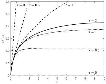
(a)

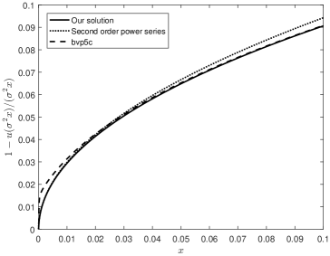
(b)

Figure 1: (a) Solutions of $\underline{\mathrm{BVP}}_{[0,L]}^{t}$ (dotted) and $\overline{\mathrm{BVP}}_{[0,L]}^{t}$ (dashed) for $L=10$ and different values of $t$. Solid line represents solution of $\mathrm{BVP}_{[0,L]}.$ (b) Comparison of $\mathrm{BVP}_{[0,L]}$ solution to solution from Matlab routine bvp5c. The displayed quantity $1-u_{L}(\sigma^{2}x)/(\sigma^{2}x)$ represents approximate implementation shortfall.

We aim to compute $u_{\infty}$ with sufficient precision on the interval $[0,1]$. The procedure has four nested loops. In the innermost loop, for a chosen time step $h$, length of the spatial interval $L\geq 1$, and number of partition points of the spatial interval $N\geq 10$ we determine the time horizon $T$ (and thus also the number of time steps $M=T/h$) in the following way. We consider two time layers, $T_{1}<T_{2}$ and the corresponding numerical solutions $u_{i}(x):=w(T_{i},x)$ for $i=1,2$, which we reparametrize in terms of relative implementation shortfall $f_{i}(x):=1-u_{i}(x)/x$. We distinguish between two regions for $x$: $\mathcal{X}=\left\{x>0:f_{2}(x)\leq 0.01\right\}$ and its complement in $[0,1]$ denoted by $\mathcal{X}^{c}$.

For small $x$, we consider relative difference in $f_{i}$. Specifically, we aim to attain

$$\sup_{x\in\mathcal{X}}\left|1-f_{2}(x)/f_{1}(x)\right|\leq 0.1.$$ (8.33)

For the remaining values of $x$ in the interval $[0,1]$ we target the absolute difference in $f_{i}$

$$\sup_{x\in\mathcal{X}^{c}}\left|f_{2}(x)-f_{1}(x)\right|\leq 10^{-4}.$$ (8.34)

We start with $T_{1}=0.1$, $T_{2}=0.2$ and increase $T_{i}$ by $0.1$ until conditions (8.33) and (8.34) are satisfied.

One level up, for given $L,h$ we start with $N_{1}=10,$ $N_{2}=20,$ denoting the corresponding solutions obtained in the innermost loop by $u_{1}$ and $u_{2}$. We increase $N_{i}$ by $10$ until conditions (8.33) and (8.34) are met again.

Two levels up, for fixed $h$ we start with $L_{1}=1$ and $L_{2}=1.1.$ We improve computational efficiency by using $u_{1}$ extended to the interval $[0,L_{2}]$ by a constant value, as the initial condition when computing $u_{2}$. We keep increasing $L_{i}$ by $0.1$ until conditions (8.33) and (8.34) are met.

In the outermost loop we check that the time step $h$ is sufficiently small so as not to have any effect on the final solution. We start with $h_{1}=10^{-5}$ and $h_{2}=0.5\times 10^{-5}$ and denote corresponding solutions determined by the previous loop by $u_{1}$ and $u_{2}$. We keep halving the time step until conditions (8.33) and (8.34) are met. Whenever possible we use previously computed values of $u$ as an initial guess for the next step of the procedure. When passing from a coarser to a finer mesh we perform this by cubic spline interpolation.

8.4 Numerical results

Recall from (3.3) that the value function satisfies

$$V(s,z) = \frac{s^{2}}{\eta\sigma^{2}}u_{\infty}(\eta\sigma^{2}\frac{z}{s})=sz\frac{u_{\infty}(\sigma^{2}x)}{\sigma^{2}x},$$

$$x = \eta\frac{z}{s}.$$ (8.35)

Here $u_{\infty}$ is the solution of $\mathrm{BVP}_{[0,\infty)}$ which in practice will be approximated by solution $\underline{\mathrm{BVP}}_{[0,L]}^{t}$ for sufficiently high $t$ and $L$ as described in Section 8.3. Breen et al. (2002) estimate linear impact of the sale of 1000 shares in a 5-minute window at around $0.18\%$ of unaffected price. If we let $z=1$ represent 1000 shares, $T=1$ one year with $n=250\times 8\times 60$ trading minutes and set the initial stock price to $s=100$ the implied value of $\eta$ turns out to be

$$\eta=0.0018\times s\times\frac{5}{n}\approx 7.5\times 10^{-6}.$$

The slightly higher estimated figure of $0.3\%$ price impact from Hasbrouck (1991, Figure IV) results in $\eta\approx 1.25\times 10^{-5}$. We set $\sigma=0.2$ in all examples.

Variable $x$ in equation (8.35) measures percentage drop in execution price assuming complete liquidation over one calendar year at a constant speed (and no accruing interest). Since $sz$ is the revenue from selling the entire inventory $z$ at price $s$ immediately and without any price impact, $I(s,z):=1-u_{\infty}(\sigma^{2}x)/(\sigma^{2}x)\$measures the percentage drop of average per-share realized price $V(s,z)/z$ relative to pre-trade price $s$. The quantity $I(s,z)$ is colloquially known as the ‘price impact’.

From (7.4) the agent’s optimal selling strategy in the original coordinates is given by

$$v(s,z)=\frac{s-V_{z}(s,z)}{2\eta}=s\frac{1-u_{\infty}^{\prime}(\eta\sigma^{2}\frac{z}{s})}{2\eta}.$$

The time to liquidation, assuming constant liquidation speed (and no accruing interest), equals

$$\tau(s,z):=\frac{z}{v(s,z)}=\frac{2x}{1-u_{\infty}^{\prime}(\sigma^{2}x)}.$$

However, the actual liquidation speed is far from constant – the asymptotic expansion (5.1) shows it to be proportional to $\sqrt{z}.$ Therefore, as a rule of thumb, $\tau(s,z)$ is roughly half of the actual average time to liquidation. This can be seen in Figure 3.

	$\sigma$	$\eta$	$s,z$	$\lambda$	$r$	$\rho$	$a$	$b$
Parametrization 1	0.2	$7.5\times 10^{-6}$	100	0	0	0.05	2	0.5
Parametrization 2	0.2	$7.5\times 10^{-6}$	100	$-0.1$	0	0	$-3$	8
Parametrization 3	0.2	$7.5\times 10^{-6}$	100	0.03	0.01	0.05	3	$-2.5$

Table 1: Parameter values used in numerical examples.

Table 1 shows three combinations of parameter values used in numerical examples. Parametrization 1 has $\lambda=r=0$, meaning that the pressure to liquidate only stems from discounting future revenues at the rate of $\rho=0.05$. Parametrization 2 has $r=\rho=0$ and the pressure to liquidate in this case stems from the unaffected asset price having a negative drift of $\lambda=-0.1$. The last parametrization has positive values of all parameters. Note that the three parametrizations also cover the three possible combinations of signs of $a$ and $b$ which allow for $a+b>0$ to be satisfied.

Part (a) of Figure 2 shows the per-share price impact $I(s,z)=1-\frac{u(\sigma^{2}x)}{\sigma^{2}x}$ for the three examples. Part (b) of the same figure shows the time to liquidation $\tau(s,z)=\frac{2x}{1-u^{\prime}(\sigma^{2}x)}$.

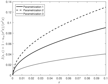
(a)

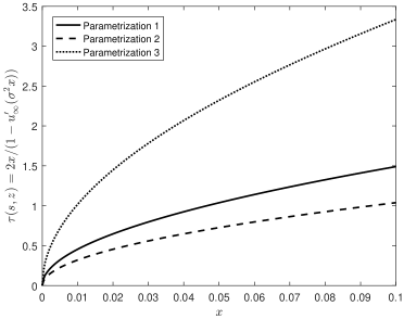
(b)

Figure 2: (a) Relative implementation shortfall; (b) Time to liquidation assuming constant liquidation speed and no accruing interest, for three parametrizations in Table 1.

Figure 3 compares the time to liquidation assuming constant liquidation speed and no accruing interest, $\tau(s,z)$, with the actual average time to liquidation, $T(Z=0)$, which was computed based on 10,000 simulations. The initial block order size is fixed at $z=100$ corresponding to 100,000 shares. The time to liquidation increases with stronger temporary price impact $\eta$ and the actual actual time to liquidation is longer than $\tau(s,z)$.

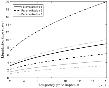
Figure 3: Actual average time to liquidation, $T(Z=0)$, based on 10,000 simulations (black lines) and approximate time to liquidation, assuming constant liquidation speed, $\tau(z,s)$, (grey lines), for three parametrizations in Table 1 and changing values of the temporary price impact parameter $\eta$.

Figure 4 shows 10,000 simulations of the liquidation with $s=z=100$ and $\eta=7.5\times 10^{-6}$ calibrated from Breen et al. (2002). All lines are shown until the (stochastic) time of liquidation, $T(Z=0)$, is reached. In the first column, we observe that, with each of the parameter sets, the execution time increases when the asset price is falling. On average, the execution takes 6.17, 4.36 and 13.80 days for the three parametrizations in Table 1, respectively.

(a)

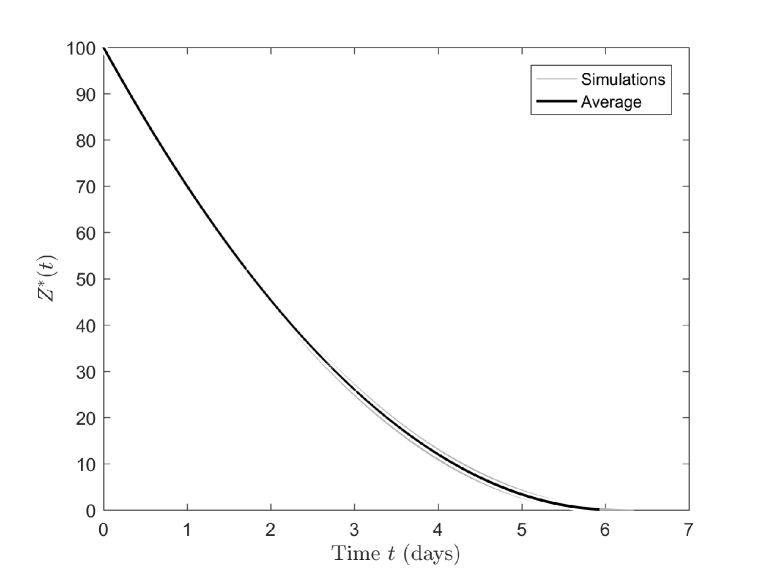
(b)

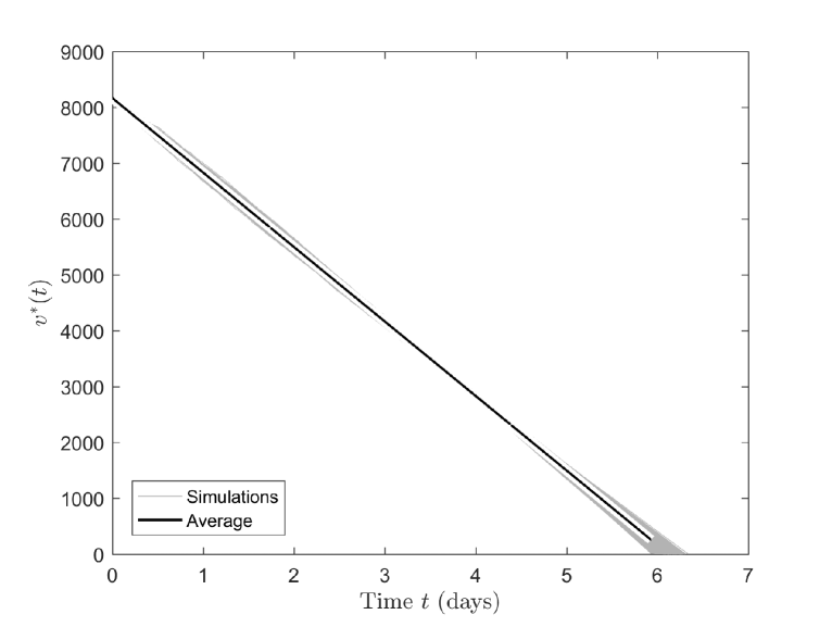
(c)

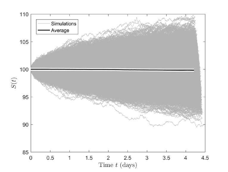
(d)

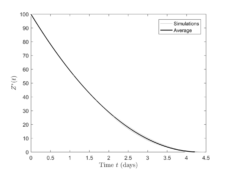
(e)

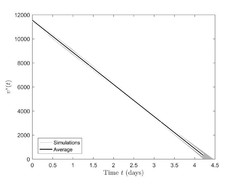
(f)

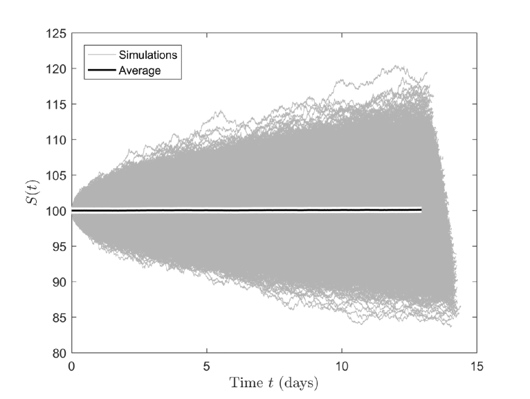
(g)

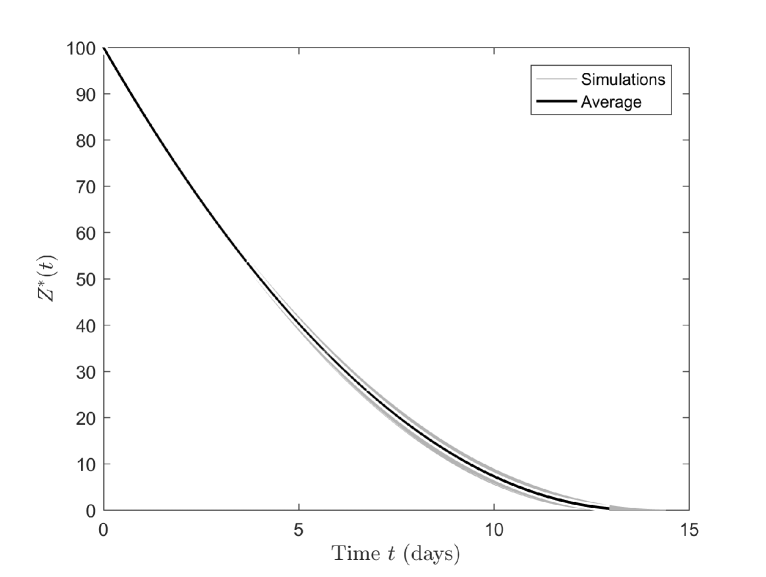
(h)

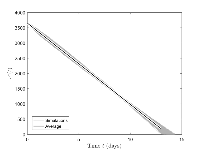
(i)

Figure 4: Each row shows 10,000 simulations of the unaffected price $S(t)$ (first column), inventory $Z^{\ast}(t)$ (second column) and the optimal strategy $v^{\ast}(t)$ (third column), for one of the three parametrizations in Table 1.

9 Conclusions

We have analyzed optimal liquidation of an asset whose unaffected price drifts downwards, while assuming that short sales of the asset are ruled out and the liquidation causes a linear temporary adverse price impact. In this setting the liquidation time horizon becomes stochastic and is determined endogenously as part of the optimal liquidation strategy. We have recovered classical result from the martingale case whereby optimal liquidation always leads to implementation shortfall, in contrast to previous studies using a fixed time horizon. While the ‘raw’ impact is linear the optimized impact is asymptotically proportional to the square root of the total volume of the order. This conclusion is well supported by empirical evidence.

The HJB equation of the new optimization gives rise to a boundary value problem whose degree of singularity is not covered in the existing literature. We have proposed a numerical scheme that overcomes the singularity and we have provided detailed theoretical analysis of the mixed boundary singular PDE our numerical scheme is based on.

For simplicity our work leaves out permanent impact and considers only linear utility. We have shown in Section 2 that in the martingale case with linear utility function the temporary and permanent impacts do not interact. In a drifting market there will be some degree of interaction, but for reasons given in Section 2 we suspect it to be rather weak. The precise nature of this interaction remains an intriguing area for future research.

Acknowlegements: We would like to thank M. Fila, P. Poláčik, P. Quittner and M. Winkler for advice concerning Sections 7 and 8. We are grateful to two anonymous referees for detailed comments and to participants of the London Mathematical Finance Seminar for their feedback. P. Brunovský thankfully acknowledges support of VEGA grant Nr. 1/0319/15. Thanks also go to VÚB Foundation for its support of A. Černý’s semester visit of Comenius University in Bratislava during which this research was initiated.

References

References

-
Almgren and Chriss (2000)
Almgren, R., Chriss, N., 2000. Optimal execution of portfolio transactions.
Journal of Risk 3, 5–39.
URL http://dx.doi.org/10.21314/JOR.2001.041 - Almgren et al. (2005) Almgren, R., Thum, C., Hauptmann, E., Li, H., 2005. Optimal execution of portfolio transactions. Risk 18 (7), 57–62.
- Anderson and Moore (1989) Anderson, B. D. O., Moore, J. B., 1989. Optimal Control: Linear Quadratic Methods. Prentice-Hall International.
-
Ankirchner et al. (2016)
Ankirchner, S., Blanchet-Scalliet, C., Eyraud-Loisel, A., 2016. Optimal
portfolio liquidation with additional information. Mathematics and Financial
Economics 10 (1), 1–14.
URL http://dx.doi.org/10.1007/s11579-015-0147-3 -
Ankirchner and Kruse (2013)
Ankirchner, S., Kruse, T., 2013. Optimal trade execution under price-sensitive
risk preferences. Quantitative Finance 13 (9), 1395–1409.
URL http://dx.doi.org/10.1080/14697688.2012.762613 - Auzinger et al. (1999) Auzinger, W., Koch, O., Kofler, P., Weinmüller, E., http://citeseerx.ist.psu.edu/viewdoc/download?doi=10.1.1.9.2179&rep=rep1&type=pdf 1999. The application of shooting to singular boundary value problems. Technical Report 126/99, Vienna University of Technology, accessed: 2014-01-31.
- Bernstein (1904) Bernstein, S., 1904. Sur certaines équations différentielles ordinaires du second ordre. Comptes Rendus de l’Académie des Sciences 138, 950–951.
-
Bershova and Rakhlin (2013)
Bershova, N., Rakhlin, D., 2013. The non-linear market impact of large trades:
evidence from buy-side order flow. Quantitative Finance 13 (11), 1759–1778.
URL http://dx.doi.org/10.1080/14697688.2013.861076 -
Bertsimas and Lo (1998)
Bertsimas, D., Lo, A. W., 1998. Optimal control of execution costs. Journal of
Financial Markets 1 (1), 1–50.
URL http://doi.org/10.1016/S1386-4181(97)00012-8 -
Breen et al. (2002)
Breen, W. J., Hodrick, L. S., Korajczyk, R. A., 2002. Predicting equity
liquidity. Management Science 48 (4), 470–483.
URL http://www.jstor.org/stable/822546 -
Brown et al. (2010)
Brown, D. B., Carlin, B. I., Lobo, M. S., 2010. Optimal portfolio liquidation
with distress risk. Management Science 56 (11), 1997–2014.
URL http://dx.doi.org/10.1287/mnsc.1100.1235 -
Brunovský et al. (2013)
Brunovský, P., Černý, A., Winkler, M., 2013. A singular
differential equation stemming from an optimal control problem in financial
economics. Applied Mathematics and Optimization 68 (2), 255–274.
URL http://dx.doi.org/10.1007/s00245-013-9205-5 -
Černý (1999)
Černý, A., 1999. Currency crises: Introduction of spot speculators.
International Journal of Finance and Economics 4 (1), 75–89.
URL http://dx.doi.org/10.1002/(SICI)1099-1158(199901)4:1<75::AID-IJFE86>3.0.CO;2-J -
Chen et al. (2015)
Chen, J., Feng, L., Peng, J., 2015. Optimal deleveraging with nonlinear
temporary price impact. European Journal of Operational Research 244 (1),
240–247.
URL http://dx.doi.org/10.1016/j.ejor.2014.12.034 -
Chen et al. (2014)
Chen, J., Feng, L., Peng, J., Ye, Y., 2014. Analytical results and efficient
algorithm for optimal portfolio deleveraging with market impact. Operations
Research 62 (1), 195–206.
URL http://dx.doi.org/10.1287/opre.2013.1222 -
Cheridito and Sepin (2014)
Cheridito, P., Sepin, T., 2014. Optimal trade execution under stochastic
volatility and liquidity. Applied Mathematical Finance 21 (4), 342–362.
URL http://dx.doi.org/10.1080/1350486X.2014.881005 - De Coster and Habets (2006) De Coster, C., Habets, P., 2006. Two-point boundary value problems: lower and upper solutions. Vol. 205 of Mathematics in Science and Engineering. Elsevier B. V., Amsterdam.
-
Donier et al. (2015)
Donier, J., Bonart, J., Mastromatteo, I., Bouchaud, J.-P., 2015. A fully
consistent, minimal model for non-linear market impact. Quantitative Finance
15 (7), 1109–1121.
URL http://dx.doi.org/10.1080/14697688.2015.1040056 -
Farmer et al. (2013)
Farmer, J. D., Gerig, A., Lillo, F., Waelbroeck, H., 2013. How efficiency
shapes market impact. Quantitative Finance 13 (11), 1743–1758.
URL http://dx.doi.org/10.1080/14697688.2013.848464 - Fleming and Soner (2006) Fleming, W. H., Soner, H. M., 2006. Controlled Markov processes and viscosity solutions, 2nd Edition. Vol. 25 of Stochastic Modelling and Applied Probability. Springer, New York.
-
Forsyth (2011)
Forsyth, P. A., 2011. A Hamilton-Jacobi-Bellman approach to optimal trade
execution. Applied Numerical Mathematics 61 (2), 241–265.
URL http://dx.doi.org/10.1016/j.apnum.2010.10.004 -
Forsyth et al. (2012)
Forsyth, P. A., Kennedy, J. S., Tse, S. T., Windcliff, H., 2012. Optimal trade
execution: a mean quadratic variation approach. Journal of Economic Dynamics
& Control 36 (12), 1971–1991.
URL http://dx.doi.org/10.1016/j.jedc.2012.05.007 -
Gatheral (2010)
Gatheral, J., 2010. No-dynamic-arbitrage and market impact. Quantitative
Finance 10 (7), 749–759.
URL http://dx.doi.org/10.1080/14697680903373692 -
Gatheral and Schied (2011)
Gatheral, J., Schied, A., 2011. Optimal trade execution under geometric
Brownian motion in the Almgren and Chriss framework. International
Journal of Theoretical and Applied Finance 14 (3), 353–368.
URL http://dx.doi.org/10.1142/S0219024911006577 -
Hasbrouck (1991)
Hasbrouck, J., 1991. Measuring the information content of stock trades. Journal
of Finance 46 (1), 179–207.
URL http://www.jstor.org/stable/2328693 -
Henderson and Hobson (2013)
Henderson, V., Hobson, D., 2013. Risk aversion, indivisible timing options, and
gambling. Operations Research 61 (1), 126–137.
URL http://dx.doi.org/10.1287/opre.1120.1131 - Henry (1981) Henry, D., 1981. Geometric theory of semilinear parabolic equations. Vol. 840 of Lecture Notes in Mathematics. Springer-Verlag, Berlin-New York.
-
Jamet (1969)
Jamet, P., 1969. On the convergence of finite-difference approximations to
one-dimensional singular boundary-value problems. Numerische Mathematik
14 (4), 355–378.
URL http://dx.doi.org/10.1007/BF02165591 -
Kyle (1985)
Kyle, A. S., 1985. Continuous auctions and insider trading. Econometrica
53 (6), 1315–1335.
URL http://www.jstor.org/stable/1913210 - Ladyzhenskaya et al. (1968) Ladyzhenskaya, O. A., Solonnikov, V. A., Uraltseva, N. N., 1968. Linear and quasilinear equations of parabolic type. Translated from the Russian by S. Smith. Translations of Mathematical Monographs, Vol. 23. American Mathematical Society, Providence, R.I.
-
Liang (2009)
Liang, J., 2009. A singular initial value problem and self-similar solutions of
a nonlinear dissipative wave equation. Journal of Differential Equations
246 (2), 819–844.
URL http://dx.doi.org/10.1016/j.jde.2008.07.022 -
Lieberman (1996)
Lieberman, G. M., 1996. Second order parabolic differential equations. World
Scientific Publishing Co., Inc., River Edge, NJ.
URL http://dx.doi.org/10.1142/3302 -
Lorenz and Almgren (2011)
Lorenz, J., Almgren, R., 2011. Mean-variance optimal adaptive execution.
Applied Mathematical Finance 18 (5), 395–422.
URL http://dx.doi.org/10.1080/1350486X.2011.560707 -
Mamer (1986)
Mamer, J. W., 1986. Successive approximations for finite horizon, semi-Markov
decision processes with application to asset liquidation. Operations Research
34 (4), 638–644.
URL http://dx.doi.org/10.1287/opre.34.4.638 - Perold (1988) Perold, A., 1988. The implementation shortfall: Paper vs. reality. Journal of Portfolio Management 14 (3), 4–9.
-
Quittner (2015)
Quittner, P., 2015. Higher order asymptotics of solutions of a singular ODE.
Asymptotic Analysis 94 (3-4), 293–308.
URL http://dx.doi.org/10.3233/ASY-151314 -
Schied (2013)
Schied, A., 2013. Robust strategies for optimal order execution in the
Almgren-Chriss framework. Applied Mathematical Finance 20 (3), 264–286.
URL http://dx.doi.org/10.1080/1350486X.2012.683963 -
Schied and Schöneborn (2009)
Schied, A., Schöneborn, T., 2009. Risk aversion and the dynamics of optimal
liquidation strategies in illiquid markets. Finance & Stochastics 13 (2),
181–204.
URL http://dx.doi.org/10.1007/s00780-008-0082-8 -
Subramanian and Jarrow (2001)
Subramanian, A., Jarrow, R. A., 2001. The liquidity discount. Mathematical
Finance 11 (4), 447–474.
URL http://dx.doi.org/10.1111/1467-9965.00124 -
Ting et al. (2007)
Ting, C., Warachka, M., Zhao, Y., 2007. Optimal liquidation strategies and
their implications. Journal of Economic Dynamics & Control 31 (4),
1431–1450.
URL http://dx.doi.org/10.1016/j.jedc.2006.07.003 -
Tóth et al. (2016)
Tóth, B., Eisler, Z., Bouchaud, J.-P., 2016. The square-root impace law
also holds for option markets. Wilmott 2016 (85), 70–73.
URL http://dx.doi.org/10.1002/wilm.10537 -
Weinmüller (1984)
Weinmüller, E., 1984. A difference method for a singular boundary value
problem of second order. Mathematics of Computation 42 (166), 441–464.
URL http://dx.doi.org/10.2307/2007595 -
Weinmüller (1986)
Weinmüller, E., 1986. On the numerical solution of singular boundary value
problems of second order by a difference method. Mathematics of Computation
46 (173), 93–117.
URL http://dx.doi.org/10.2307/2008217