Computing period matrices and the Abel-Jacobi map of superelliptic curves

1 Introduction

The Abel-Jacobi map links a complex curve to a complex torus. In particular the matrix of periods allows to define the Riemann theta function of the curve, which is an object of central interest in mathematics and physics: let us mention the theory of abelian functions or integration of partial differential equations.

In the context of cryptography and number theory, periods also appear in the BSD conjecture or as a tool to identify isogenies or to find curves having prescribed complex multiplication [22]. For such diophantine applications, it is necessary to compute integrals to large precision (say thousand digits) and to have rigorous results.

1.1 Existing algorithms and implementations

For genus 1 and 2, methods based on isogenies (AGM [7], Richelot [3], Borchardt mean [14]) make it possible to compute periods to arbitrary precision in almost linear time. However, these techniques scale very badly when the genus grows.

For modular curves, the modular symbols machinery and termwise integration of expansions of modular forms give excellent algorithms [16, §3.2].

For hyperelliptic curves of arbitrary genus, the Magma implementation due to van Wamelen [22] computes period matrices and the Abel-Jacobi map. However, it is limited in terms of precision (less than $2000$ digits) and some bugs are experienced on certain configurations of branch points. The shortcomings of this implementation motivated our work. Using a different strategy (integration along a tree instead of around Voronoi cells) we obtain a much faster, more reliable algorithm and rigorous results.

For general algebraic curves, there is an implementation in Maple due to Deconinck and van Hoeij [8]. We found that this package is not suitable for high precision purposes.

We also mention the Matlab implementations due to Frauendiener and Klein for hyperelliptic curves [10] and for general algebraic curves [9].

Moreover, a Sage implementation for general algebraic curves due to Nils Bruin and Alexandre Zotine is in progress.

1.2 Main result

This paper adresses the problem of computing period matrices and the Abel-Jacobi map of algebraic curves given by an affine equation of the form (see Definition LABEL:m-def:se_curve)

$$y^{m}=f(x),\quad m>1,f\in\mathbb{C}[x]\text{ separable of degree}\operatorname{deg}(f)=n\geq 3.$$

They generalize hyperelliptic curves and are usually called superelliptic curves.

We take advantage of their specific geometry to obtain the following (see Theorem LABEL:m-thm:complexity_integrals)

Theorem 1.1.

Let $\mathcal{C}$ be a superelliptic curve of genus $g$ defined by an equation $y^{m}=f(x)$ where $f$ has degree $n$. We can compute a basis of the period lattice to precision $D$ using

$$O(n(g+\log D)(g+D)^{2}\log^{2+\varepsilon}(g+D))\text{ binary operations,}$$

where $\epsilon>0$ is chosen so that the multiplication of precision $D$ numbers has complexity $O(D\log^{1+\epsilon}D)$.

1.3 Rigorous implementation

The algorithm has been implemented in C using the Arb library [11]. This system represents a complex numbers as a floating point approximation plus an error bound, and automatically takes into account all precision loss occurring through the execution of the program. With this model we can certify the accuracy of the numerical results of our algorithm (up to human or even compiler errors, as usual).

Another implementation has been done in Magma [2]. Both are publicly available on github at https://github.com/pascalmolin/hcperiods [19].

1.4 Interface with the LMFDB

Having rigorous period matrices is a valuable input for the methods developed by Sijsling et al. [6] to compute endormorphism rings of Jacobians of hyperelliptic curves. During a meeting aimed at expanding the ‘L-functions and modular forms database’ [15, LMFDB] to include genus $3$ curves, the Magma implementation of our algorithm was incorporated in their framework to successfully compute the endomorphism rings of Jacobians of $67,879$ hyperelliptic curves of genus $3$, and confirm those of the $66,158$ genus 2 curves that are currently in the database.

For these applications big period matrices were computed to $300$ digits precision.

1.5 Structure of the paper

In Section LABEL:m-sec:ajm we briefly review the objects we are interested in, namely period matrices and the Abel-Jacobi map of nice algebraic curves. The ingredients to obtain these objects, a basis of holomorphic differentials and a homology basis, are made explicit in the case of superelliptic curves in Section LABEL:m-sec:se_curves. We give formulas for the computation of periods in Section LABEL:m-sec:strat_pm and explain how to obtain from them the standard period matrices using symplectic reduction. In Section 5 we give explicit formulas for the intersection numbers of our homology basis. For numerical integration we employ two different integration schemes that are explained in Section LABEL:m-sec:numerical_integration: the double-exponential integration and (in the case of hyperelliptic curves) Gauss-Chebychev integration. The actual computation of the Abel-Jacobi map is explained in detail in Section LABEL:m-sec:comp_ajm. In Section LABEL:m-sec:comp_asp we analyze the complexity of our algorithm and share some insights on the implementation. Section LABEL:m-sec:examples_timings contains some tables with running times to demonstrate the performance of the code. Finally, in Section LABEL:m-sec:outlook we conclude with an outlook on what can be done in the future.

1.6 Acknowledgements

The first author wants to thank the crypto team at Inria Nancy, where a first version of this work was carried out in the case of hyperelliptic curves. He also acknowledges the support from Partenariat Hubert Curien under grant 35487PL.

The second author wants to thank Steffen Müller and Florian Hess for helpful discussions. Moreover, he acknowledges the support from DAAD under grant 57212102.

2 The Abel-Jacobi map

We recall, without proof, the main objects we are interested in, and which will become completely explicit in the case of superelliptic curves. The exposition follows that of [21, Section 2].

2.1 Definition

Let $\mathcal{C}$ be a smooth irreducible projective curve of genus $g>0$. Its space of holomorphic differentials $\Omega^{1}_{\mathcal{C}}$ has dimension $g$; let us fix a basis $\omega_{1},\dots\omega_{g}$ and denote by $\bar{\omega}$ the vector $(\omega_{1},\dots\omega_{g})$.

For any two points $P,Q\in\mathcal{C}$ we can consider the vector integral $\int_{P}^{Q}\bar{\omega}\in\mathbb{C}^{g}$, whose value depends on the chosen path from $P$ to $Q$.

In fact, the integral depends on the path up to homology, so we introduce the period lattice of $\mathcal{C}$

$$\Lambda=\left\{\int_{\gamma}\omega_{j},\gamma\in H_{1}(\mathcal{C},\mathbb{Z})\right\}\subset\mathbb{C}^{g},$$

where $H_{1}(\mathcal{C},\mathbb{Z})\cong\mathbb{Z}^{2g}$ is the first homology group of the curve.

Now the integral

$$P,Q\mapsto\int_{P}^{Q}\bar{\omega}\in\mathbb{C}^{g}/\Lambda$$

is well defined, and the definition can be extended by linearity to the group of degree zero divisors

$$\operatorname{Div}^{0}(\mathcal{C})=\left\{\sum a_{i}P_{i},a_{i}\in\mathbb{Z},\sum a_{i}=0\right\}.$$

The Abel-Jacobi theorem states that one obtains a surjective map whose kernel is formed by divisors of functions, so that the integration provides an explicit isomorphism

$$\mathcal{A}:\left\{\begin{array}[]{ccc}\operatorname{Jac}(\mathcal{C})=\operatorname{Div}^{0}(\mathcal{C})/\operatorname{Prin}^{0}(\mathcal{C})&\longrightarrow&\mathbb{C}^{g}/\Lambda\\ \sum_{i}[Q_{i}-P_{i}]&\mapsto&\sum_{k}\int_{P_{i}}^{Q_{i}}\bar{\omega}\mod\Lambda\end{array}\right.$$

between the Jacobian variety and the complex torus.

2.2 Explicit basis and standard matrices

Let us choose a symplectic basis of $H_{1}(\mathcal{C},\mathbb{Z})$, that is two families of cycles $\alpha_{i}$, $\beta_{j}$ for $1\leq i,j\leq g$ such that the intersections satisfy

$$\left(\alpha_{i}\circ\beta_{j}\right)=\delta_{i,j},$$

the other intersections all being zero.

We define the period matrices on those cycles

$$\Omega_{A}=\left(\int_{\alpha_{i}}\omega_{j}\right)_{1\leq i,j\leq g}\text{ and }\Omega_{B}=\left(\int_{\beta_{i}}\omega_{j}\right)_{1\leq i,j\leq g}$$

and call the concatenated matrix

$$\Omega=(\Omega_{A},\Omega_{B})\in\mathbb{C}^{g\times 2g}$$

such that $\Lambda=\Omega\mathbb{Z}^{2g}$ a big period matrix.

If one takes as basis of differentials the dual basis of the cycles $\alpha_{i}$, the matrix becomes

$$\Omega_{A}^{-1}\Omega=(I_{g},\tau),$$

where $\tau=\Omega_{A}^{-1}\Omega_{B}\in\mathbb{C}^{g\times g}$, called a small period matrix, is in the Siegel space $\mathcal{H}_{g}$ of symmetric matrices with positive definite imaginary part.

3 Superelliptic curves

3.1 Definition & properties

Definition 3.1.

In this paper, a superelliptic curve $\mathcal{C}$ over $\mathbb{C}$ is a smooth projective curve that has an affine model given by an equation of the form

$$\mathcal{C}_{\text{aff}}:\quad y^{m}=f(x)=c_{f}\cdot\prod_{k=1}^{n}(x-x_{k}),$$ (1)

where $m>1$ and $f\in\mathbb{C}[x]$ is separable of degree $n\geq 3$. Note that we do not assume that $\gcd(m,n)=1$.

There are $\delta=\gcd(m,n)$ points $P_{\infty}^{(1)},\dots,P_{\infty}^{(\delta)}\in\mathcal{C}$ at infinity, that behave differently depending on $m$ and $n$ (see [20, §1] for details). In particular, $\infty\in\mathbb{P}^{1}_{\mathbb{C}}$ is a branch point for $\delta\neq m$. Thus, we introduce the set of finite branch points $X=\{x_{1},\dots,x_{d}\}$ as well as the set of all branch points

$$\hat{X}=\begin{cases}X\cup\{\infty\}\quad\text{if}\;m\nmid d,\\ X\hfill\text{otherwise.}\end{cases}$$ (2)

The ramification indices at the branch points are given by $e_{x}=m$ for all $x\in X$ and $e_{\infty}=\frac{m}{\delta}$. Using the Riemann-Hurwitz formula, we obtain the genus of $\mathcal{C}$ as

$$g=\frac{1}{2}((m-1)(n-1)-\delta+1).$$ (3)

We denote the corresponding finite ramification points $P_{k}=(x_{k},0)\in\mathcal{C}$ for $k=1,\dots,n$.

Remark 3.2.

Without loss of generality we may assume $c_{f}=1$ (if not, apply the transformation $(x,y)\mapsto(x,\sqrt[m]{c_{f}}y)$).

Remark 3.3.

For any $\begin{pmatrix}a&b\\ c&d\end{pmatrix}\in\operatorname{PSL}(2,\mathbb{C})$, the Moebius transform $\phi:u\mapsto\frac{au+b}{cu+d}$ is an automorphism of $\mathbb{P}^{1}$. By a change of coordinate $x=\phi(u)$ we obtain a different model of $\mathcal{C}$ given by the equation

$$\tilde{v}^{m}=\tilde{f}(u)$$

where $\tilde{f}(u)=f(\phi(u))(cu+d)^{\ell m}$ and $v=y(cu+d)^{\ell}$ for the smallest value $\ell$ such that $\ell m\geq n$.

If the curve was singular at infinity, the singularity is moved to $u=-d/c$ in the new model. This happens when $\delta<m$ (so that $\ell m>n$).

When $\delta=m$ we may apply such a transformation to improve the configuration of affine branch points.

3.2 Complex roots and branches of the curve

3.2.1 The complex $m$-th root

Working over the complex numbers we encounter several multi-valued functions which we will briefly discuss here. Closely related to superelliptic curves over $\mathbb{C}$ is the complex $m$-th root. Before specifying a branch it is a multi-valued function $y^{m}=x$ that defines an $m$-sheeted Riemann surface, whose only branch points are at $x=0,\infty$, and these are totally ramified.

For $x\in\mathbb{C}$, it is natural and computationally convenient to use the principal branch of the $m$-th root $\sqrt[m]{x}$ defined by

$$-\frac{\pi}{m}<\arg(\sqrt[m]{x})\leq\frac{\pi}{m}$$

which has a branch cut along the negative real axis $]\!-\infty,0]$. Crossing it in positive orientation corresponds to multiplication by the primitive $m$-th root of unity

$$\zeta:=\zeta_{m}:=e^{\frac{2\pi i}{m}}$$

on the surface. In particular, the monodromy at $x=0$ is cyclic of order $m$.

3.2.2 The Riemann surface

For an introduction to the theory of Riemann surfaces, algebraic curves and holomorphic covering maps we recommend [17].

Over $\mathbb{C}$ we can identify the curve $\mathcal{C}$ with the compact Riemann surface $\mathcal{C}(\mathbb{C})$. Since our defining equation has the nice form $y^{m}=\prod_{k=1}^{n}(x-x_{k})$ we view $\mathcal{C}$ as a Riemann surface with $m$ sheets and all computations will be done in the $x$-plane.

We denote by $\operatorname{pr_{x}}:\mathcal{C}\rightarrow\mathbb{P}^{1}_{\mathbb{C}}$ the corresponding smooth cyclic branched covering of the projective line defined by the $x$-coordinate.

There are $m$ possibilities to continue $y$ as an analytic function following a path in the $x$-plane. This is crucial for the integration of differentials on $\mathcal{C}$. Due to the cyclic structure of $\mathcal{C}$, they are related in a convenient way:

We call a branch of $\mathcal{C}$ a function $y(x)$ such that $y(x)^{m}=f(x)$ for all $x\in\mathbb{C}$. At every $x$, the branches of $\mathcal{C}$ only differ by a factor $\zeta^{l}$ for some $l\in\{0,\dots,m-1\}$. Thus, following a path, it is sufficient to know one branch that is analytic in a suitable neighborhood. In the next paragraph, we will introduce locally analytic branches very explicitly.

Similar to the complex $m$-th root, we can assume that crossing the branch cut at $x_{k}\in X$ in positive direction corresponds to multiplication by $\zeta$ on the Riemann surface. We obtain an ordering of the sheets relative to the analytic branches of $\mathcal{C}$ by imposing that multiplication by $\zeta$, i.e. applying the map $(x,y(x))\mapsto(x,\zeta y(x))$, corresponds to moving one sheet up on the Riemann surface.

Consequently, the local monodromy of the cyclic covering $\operatorname{pr_{x}}$ is equal and cyclic of order $m$ at every $x_{k}\in X$ and the monodromy group is, up to conjugation, the cyclic group $C_{m}$. This makes it possible to find explicit generators for the homology group $H_{1}(\mathcal{C},\mathbb{Z})$ without specifying a base point, as shown in §LABEL:m-subsec:cycles_homo.

3.2.3 Locally analytic branches

In order to integrate differential forms on $\mathcal{C}$ it is sufficient to be able to follow one explicit analytic continuation of $y$ along a path joining two branch points $a,b\in X$.

One could of course consider the principal branch of the curve

$$y(x)=\sqrt[m]{f(x)},$$

but this is not a good model to compute with: it has branch cuts wandering around the $x$-plane (see Figure 1a).

A better option is to split the product as follows: assume that $(a,b)=(-1,1)$. Then the function

$$y(x)=\prod_{x_{k}\in X}\sqrt[m]{x-x_{k}}$$

has $n$ branch cuts parallel to the real line (see Figure 1b). However, one of them lies exactly on the interval $[-1,1]$ we are interested in. We work around this by taking the branch cut towards $+\infty$ for each branch point $x_{k}$ with positive real part, writing

$$y(x)=e^{\frac{i\pi r^{+}}{m}}\prod_{\operatorname{Re}(x_{k})\leq 0}\sqrt[m]{x-x_{k}}\prod_{\operatorname{Re}(x_{k})>0}\sqrt[m]{x_{k}-x},$$

where $r^{+}$ is the number of points with positive real part.

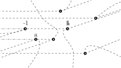
(a) principal branch

(b) product

(c) $y_{a,b}$

Figure 1: Branch cuts of different $m$-th roots.

In general we proceed in the same way: For branch points $a,b\in X$ we consider the affine linear transformation

$$x_{a,b}:u\mapsto\frac{b-a}{2}\left(u+\frac{b+a}{b-a}\right),$$

which maps $[-1,1]$ to the complex line segment $[a,b]$, and denote the inverse map by

$$u_{a,b}:x\mapsto\frac{2x-a-b}{b-a}.$$

We split the image of the branch points under $u_{a,b}$ into the following subsets

$$\left\{u_{a,b}(x),x\in X\right\}=\left\{-1,1\right\}\cup U^{+}\cup U^{-},$$ (4)

where points in $U^{+}$ (resp. $U^{-}$) have strictly positive (resp. non-positive) real part.

Then the product

$$\tilde{y}_{a,b}(u)=\prod_{u_{k}\in U^{-}}\sqrt[m]{u-u_{k}}\prod_{u_{k}\in U^{+}}\sqrt[m]{u_{k}-u}$$ (5)

is holomorphic on a neighborhood $\varepsilon_{a,b}$ of $[-1,1]$ which we can take as an ellipse containing no point $u_{k}\in U^{-}\cup U^{+}$, while the term corresponding to $a,b$

$$\sqrt[m]{1-u^{2}}$$

has two branch cuts $]-\infty,-1]$ and $[1,\infty[$, and is holomorphic on the complement $\overline{U}$ of these cuts.

We can now define a branch of the curve

$$y_{a,b}(x)=C_{a,b}\tilde{y}_{a,b}(u_{a,b}(x))\sqrt[m]{1-u_{a,b}(x)^{2}}$$ (6)

by setting $r=1+\#U^{+}\bmod 2$ and choosing the constant

$$C_{a,b}=\left(\frac{b-a}{2}\right)^{\frac{n}{m}}e^{\frac{\pi i}{m}r}$$ (7)

such that $y_{a,b}(x)^{m}=f(x)$.

The function $y_{a,b}(x)$ has $n$ branch cuts all parallel to $[a,b]$ in outward direction and is holomorphic inside $]a,b[$ (see Figure 1c).

More precisely, $V_{a,b}=u_{a,b}(\varepsilon_{a,b}\cap\overline{U}_{a,b})$, is an ellipse-shaped neighborhood of $]a,b[$ with two segments removed (see Figure LABEL:m-fig:set_vab) on which the local branch $y_{a,b}$ is well defined and holomorphic.

Figure 2: Holomorphic neighborhood of $y_{a,b}$.

We sum up the properties of these local branches:

Proposition 3.4.

Let $a,b\in X$ be branch points such that $X\cap\,]a,b[\,=\varnothing$. Then, with the notation as above, the functions $\tilde{y}_{a,b}$ (5) and $y_{a,b}$ (6) satisfy

• $\tilde{y}_{a,b}$ is holomorphic and does not vanish on $\varepsilon_{a,b}$,

• $y_{a,b}(x)=C_{a,b}\tilde{y}_{a,b}(u_{a,b}(x))\sqrt[m]{1-u_{a,b}(x)^{2}}$ is holomorphic on $V_{a,b}$,

• $y_{a,b}(x)^{m}=f(x)$ for all $x\in\mathbb{C}$,

• $y_{a,b}(x),\zeta y_{a,b}(x),\dots,\zeta^{m-1}y_{a,b}(x)$ are the $m$ different analytic continuations of $y$ on $V_{a,b}$.

Moreover, we can assume that for $x\in V_{a,b}$, applying the map $(x,y_{a,b}(x))\mapsto(x,\zeta^{l}y_{a,b}(x))$ corresponds to moving up $l\in\mathbb{Z}/m\mathbb{Z}$ sheets on the Riemann surface.

3.3 Cycles and homology

For us, a cycle on $\mathcal{C}$ is a smooth oriented closed path in $\pi_{1}(\mathcal{C})$. For simplicity we identify all cycles with their homology classes in $H_{1}(\mathcal{C},\mathbb{Z})=\pi_{1}(\mathcal{C})/[\pi_{1}(\mathcal{C}),\pi_{1}(\mathcal{C})]$.

In the following we present an explicit generating set of $H_{1}(\mathcal{C},\mathbb{Z})$ that relies on the locally analytic branches $y_{a,b}$ as defined in (LABEL:m-eq:def_yab) and the superelliptic structure of $\mathcal{C}$.

Let $a,b\in X$ be branch points such that $X\cap]a,b[=\varnothing$, where $[a,b]$ is the oriented line segment connecting $a$ and $b$.

By Proposition LABEL:m-prop:yab the lifts of $[a,b]$ to $\mathcal{C}$ are given by

$$\gamma^{(l)}_{[a,b]}=\{(x,\zeta^{l}y_{a,b}(x))\mid x\in[a,b]\},\quad l\in\mathbb{Z}/m\mathbb{Z}.$$

These are smooth oriented paths that connect $P_{a}=(a,0)$ and $P_{b}=(b,0)$ on $\mathcal{C}$. We obtain cycles by concatenating these lifts in the following way:

$$\gamma_{a,b}^{(l)}=\gamma^{(l)}_{[a,b]}\cup\gamma^{(l+1)}_{[b,a]}\in\pi_{1}(\mathcal{C}).$$ (8)

Definition 3.5 (Elementary cycles).

We say $\gamma_{a,b}=\gamma_{a,b}^{(0)}$ is an elementary cycle and call $\gamma_{a,b}^{(l)}$ its shifts for $l\in\mathbb{Z}/m\mathbb{Z}$.

In $\pi_{1}(\mathcal{C})$ shifts of elementary cycles are homotopic to cycles that encircle $a$ in negative and $b$ in positive orientation, once each. By definition of $y_{a,b}$ the branch cuts at the end points are outward and parallel to $[a,b]$. Thus, we have the following useful visualizations of $\gamma_{a,b}^{(l)}$ on $\mathcal{C}$:

Figure 3: Representations of a cycle $\gamma_{a,b}^{(l)}$.

As it turns out, we do not need all elementary cycles and their shifts to generate $H_{1}(\mathcal{C},\mathbb{Z})$, but only those that correspond to edges in a spanning tree, that is a subset $E\in X\times X$ of directed edges $(a,b)$ such that all branch points are connected without producing any cycle. It must contain exactly $n-1$ edges. The actual tree will be chosen in §4.3 in order to minimize the complexity of numerical integration.

For an edge $e=(a,b)\in E$, we denote by $\gamma_{e}^{(l)}$ the shifts of the corresponding elementary cycle $\gamma_{a,b}$.

Theorem 3.6.

Let $E$ be a spanning tree for the branch points $X$. The set of cycles $\Gamma=\left\{\gamma_{e}^{(l)}\mid 0\leq l<m-1,e\in E\right\}$ generates $H_{1}(\mathcal{C},\mathbb{Z})$.

Proof.

Denote by $\alpha_{a}\in\pi_{1}(\mathbb{P}^{1}\setminus\hat{X})$ a closed path that encircles the branch point $a\in\hat{X}$ exactly once. Then, due to the relation $1=\prod_{a\in\hat{X}}\alpha_{a}$, $\pi_{1}(\mathbb{P}^{1}\setminus\hat{X})$ is freely generated by $\{\alpha_{a}\}_{a\in X}$, i.e. in the case $\delta\neq m$ we can omit $\alpha_{\infty}$.
Since our covering is cyclic, we have that $\pi_{1}(\mathcal{C}\setminus\operatorname{pr_{x}}^{-1}(\hat{X}))\cong\ker(\pi_{1}(\mathbb{P}^{1}\setminus\hat{X})\overset{\Phi}{\longrightarrow}\operatorname{Aut}(\mathcal{C}\setminus\operatorname{pr_{x}}^{-1}(\hat{X})))$ where $\operatorname{Aut}(\mathcal{C}\setminus\operatorname{pr_{x}}^{-1}(\hat{X}))\cong C_{m}\subset S_{m}$ and $\Phi(\alpha_{a})$ is cyclic of order $m$ for all $a\in X$. Hence, for every word $\alpha=\alpha_{1}^{s_{1}}\dots\alpha_{n}^{s_{n}}\in\pi_{1}(\mathbb{P}^{1}\setminus\hat{X})$ we have that $\alpha\in\ker(\Phi)\Leftrightarrow\sum_{i=1}^{n}s_{i}\equiv 0\bmod m$.
We now claim that $\pi_{1}(\mathcal{C}\setminus\operatorname{pr_{x}}^{-1}(\hat{X}))=\langle\alpha_{a}^{-s}\alpha_{b}^{s},\alpha_{a}^{m}\mid s\in\mathbb{Z},a,b\in X\rangle$ and prove this by induction on $n$: for $\alpha=\alpha_{1}^{s_{1}}$, $m$ divides $s_{1}$ and therefore $\alpha$ is generated by $\alpha_{1}^{m}$. For $n>1$ we write $\alpha=\alpha_{1}^{s_{1}}\dots\alpha_{n}^{s_{n}}=(\alpha_{1}^{s_{1}}\dots\alpha_{n-1}^{s_{n-1}+s_{n}})(\alpha_{n-1}^{-s_{n}}\alpha_{n}^{s_{n}})$.
We obtain the fundamental group of $\mathcal{C}$ as $\pi_{1}(\mathcal{C})\cong\pi_{1}(\mathcal{C}\setminus\operatorname{pr_{x}}^{-1}(\hat{X}))/\langle\alpha_{a}^{e_{a}}\mid a\in\hat{X}\rangle$, which is generated by $\{\alpha_{a}^{-s}\alpha_{b}^{s}\mid s\in\mathbb{Z}/m\mathbb{Z},a,b\in X\}$.
All branch points $a,b\in X$ are connected by a path $(a,v_{1},\dots,v_{t},b)$ in the spanning tree, so we can write $\alpha_{a}^{-s}\alpha_{b}^{s}=(\alpha_{a}^{-s}\alpha_{v_{1}}^{s})(\alpha_{v_{1}}^{-s}\alpha_{v_{2}}^{s})\dots(\alpha_{v_{t-1}}^{-s}\alpha_{v_{t}}^{s})(\alpha_{v_{t}}^{-s}\alpha_{b}^{s})$ and hence we have that $\{\alpha_{a}^{-s}\alpha_{b}^{s}\mid s\in\mathbb{Z}/m\mathbb{Z},(a,b)\in E\}$ generates $\pi_{1}(\mathcal{C})$ and therefore $H_{1}(\mathcal{C},\mathbb{Z})$.
If we choose basepoints $p_{0}\in\mathbb{P}^{1}\setminus\hat{X}$ for $\pi_{1}(\mathbb{P}^{1}\setminus\hat{X})$ and $P_{0}\in\operatorname{pr_{x}}^{-1}(p_{0})$ for $\pi_{1}(\mathcal{C}\setminus\operatorname{pr_{x}}^{-1}(\hat{X}))$ and $\pi_{1}(\mathcal{C})$ respectively, then, depending on the choice of $P_{0}$, for all $e=(a,b)\in E$ there exists $l_{0}\in\mathbb{Z}/m\mathbb{Z}$ such that $\gamma_{e}^{(l_{0})}$ is homotopic to $\alpha_{a}^{-1}\alpha_{b}$ in $\pi_{1}(\mathcal{C},P_{0})$. In $H_{1}(\mathcal{C},\mathbb{Z})$ we have that $\alpha_{a}^{-s}\alpha_{b}^{s}=(\alpha_{a}^{-1}\alpha_{b})^{s}$, so we obtain the other powers by concatenating the shifts $\prod_{l=0}^{s-1}\gamma_{e}^{(l_{0}+l)}=(\alpha_{a}^{-1}\alpha_{b})^{s}$. This implies $1=\prod_{l=0}^{m-1}\gamma_{e}^{(l_{0}+l)}=\prod_{l=0}^{m-1}\gamma_{e}^{(l)}$ and

$$\{\alpha_{a}^{-s}\alpha_{b}^{s}\mid s\in\mathbb{Z}/m\mathbb{Z}\}\subset\langle\gamma_{e}^{(l)}\mid 0\leq l<m-1\rangle,$$

and therefore $H_{1}(\mathcal{C},\mathbb{Z})=\langle\Gamma\rangle$. ∎

Remark 3.7.

• For $\delta=1$, we have that $\#\Gamma=(m-1)(n-1)=2g$. Therefore, $\Gamma$ is a basis for $H_{1}(\mathcal{C},\mathbb{Z})$ in that case.

• In the case $\delta=m$, the point at infinity is not a branch point. Leaving out one finite branch point in the spanning tree results in only $n-2$ edges. Hence, we easily find a subset $\Gamma^{\prime}\subset\Gamma$ such that $\#\Gamma^{\prime}=(m-1)(n-2)=2g$ and $\Gamma^{\prime}$ is a basis for $H_{1}(\mathcal{C},\mathbb{Z})$.

3.4 Differential forms

The computation of the period matrix and the Abel-Jacobi map requires a basis of $\Omega^{1}_{\mathcal{C}}$ as a $\mathbb{C}$-vector space. In this section we provide a basis that only depends on $m$ and $n$ and is suitable for numerical integration.
Among the meromorphic differentials

$$\mathcal{W}^{\text{mer}}=\left\{\omega_{i,j}\right\}_{\begin{subarray}{c}1\leq i\leq n-1,\\ 1\leq j\leq m-1\end{subarray}}\quad\text{with}\quad\omega_{i,j}=\frac{\mathrm{d}x^{i}}{iy^{j}},$$

there are exactly $g$ that are holomorphic and they can be found by imposing a simple combinatorial condition on $i$ and $j$. The following proposition is basically a more general version of [20, Proposition 2].

Proposition 3.8.

Let $\delta=\gcd(m,n)$. The following differentials form a $\mathbb{C}$-basis of $\Omega^{1}_{\mathcal{C}}$:

$$\mathcal{W}=\left\{\omega_{i,j}\in\mathcal{W}^{\text{mer}}\mid-mi+jn-\delta\geq 0\right\}$$

Proof.

First we show that the differentials in $\mathcal{W}$ are holomorphic. Let $\omega_{i,j}=x^{i-1}y^{-j}\mathrm{d}x\in\mathcal{W}^{\text{mer}}$. We write down the relevant divisors

$$\operatorname{div}(x) =\sum_{k=1}^{m}\left(0,\zeta^{k}\sqrt[m]{f(0)}\right)-\frac{m}{\delta}\cdot\sum_{l=1}^{\delta}P_{\infty}^{(l)},$$

$$\operatorname{div}(y) =\sum_{k=1}^{n}P_{k}-\frac{n}{\delta}\cdot\sum_{l=1}^{\delta}P_{\infty}^{(l)},$$

$$\operatorname{div}(\mathrm{d}x) =(m-1)\sum_{k=1}^{n}P_{k}-\left(\frac{m}{\delta}+1\right)\cdot\sum_{l=1}^{\delta}P_{\infty}^{(l)}.$$

Putting together the information, for $P\in\mathcal{C}$ lying over $x_{0}\in\mathbb{P}^{1}_{\mathbb{C}}$, we obtain

$$v_{P}(\omega_{i,j}) =(i-1)v_{P}(x)+v_{P}(\mathrm{d}x)-jv_{P}(y)\begin{cases}\geq 0\hfill\text{if}\;x_{0}\neq x_{k},\infty,\\ =m-1-j\geq 0\quad\text{if}\;x_{0}=x_{k},\\ =\frac{(-mi-\delta+jn)}{\delta}\hfill\text{if}\;x_{0}=\infty.\end{cases}$$ (9)

We conclude: $\omega_{i,j}\in\mathcal{W}^{\text{mer}}$ is holomorphic if and only if $\omega_{i,j}\in\mathcal{W}$.
Since the differentials in $\mathcal{W}$ are clearly $\mathbb{C}$-linearly independent, it remains to show that there are enough of them, i.e. $\#\mathcal{W}=g$.

Counting the elements in $\mathcal{W}$ corresponds to counting lattice points $(i,j)\in\mathbb{Z}^{2}$ in the trapezoid given by the faces

$$1\leq i\leq n-1,$$

$$1\leq j\leq m-1,$$

$$i\leq\frac{n}{m}j-\frac{\delta}{m}.$$

Figure 4: The points below the line correspond to holomorphic differentials. Illustrated is the case $n=4,m=8$, and thus $g=9$.

Summing over the vertical lines of the trapezoid, we find the following formula that counts the points.

$$\#\mathcal{W} =\sum_{j=1}^{m-1}\left\lfloor\frac{n}{m}j-\frac{\delta}{m}\right\rfloor=\sum_{j=1}^{m-1}\frac{nj-\delta-r_{j}}{m}=\frac{n}{m}\sum_{j=1}^{m-1}j-\frac{m-1}{m}\delta-\frac{1}{m}\sum_{j=1}^{m-1}r_{j},$$ (10)

where $r_{j}=nj-\delta\bmod m$.

The desired equality $\#\mathcal{W}=\frac{1}{2}((n-1)(m-1)-\delta+1)=g$ immediately follows from

Lemma 3.9.

$$\sum_{j=1}^{m-1}r_{j}=\frac{1}{2}(m^{2}-(\delta+2)m+2\delta).$$

Proof.

Let $l:=\frac{m}{\delta}$. First we note that $r_{j}=r_{j+l}$:

$$r_{j+l}=n(j+l)-\delta\bmod m=nj+\frac{n}{\delta}m-\delta\bmod m=nj-\delta\bmod m=r_{j},$$

and hence

$$\sum_{j=1}^{m-1}r_{j}=\delta\cdot\sum_{j=1}^{l}r_{j}-r_{m}=\delta\cdot\sum_{j=1}^{l}r_{j}-(-\delta+m).$$ (11)

Furthermore, $r_{j}$ can be written as a multiple of $\delta$:

$$r_{j}=\delta\left(\frac{n}{\delta}j-1\right)\bmod m.$$

From $\gcd(\frac{n}{\delta},l)=1$ we conclude $\left\{\frac{n}{\delta}j-1\bmod l\mid 1\leq j\leq l\right\}=\{0,\dots,l-1\}$. Therefore,

$$\sum_{j=1}^{l}r_{j}=\sum_{j=0}^{l-1}\delta j=\delta\cdot\frac{l(l-1)}{2},$$ (12)

and thus (LABEL:m-eq:r_j3) and (LABEL:m-eq:r_j4) imply

$$\sum_{j=1}^{m-1}r_{j}=\delta\cdot\sum_{j=1}^{l}r_{j}+\delta-m=\delta^{2}\cdot\frac{l(l-1)}{2}+\delta-m=\frac{1}{2}(m^{2}-(\delta+2)m+2\delta).$$

∎

Remark 3.10.

Note that from (LABEL:m-eq:diff_cases) it follows that the meromorphic differentials in $\mathcal{W}^{\text{mer}}$ are homolorphic at all finite points.

4 Strategy for the period matrix

In this section we present our strategy to obtain period matrices $\Omega_{\Gamma},\Omega_{A},\Omega_{B}$ and $\tau$ as defined in §LABEL:m-subsec:bases_matrices. Although this paper is not restricted to the case $\gcd(m,n)=1$, we will briefly assume it in this paragraph to simplify notation.

The main ingredients were already described in Section LABEL:m-sec:se_curves: we integrate the holomorphic differentials in $\mathcal{W}$ (§LABEL:m-subsec:diff_forms) over the cycles in $\Gamma$ (§LABEL:m-subsec:cycles_homo) using numerical integration (§6.1), which results in a period matrix (§LABEL:m-subsec:comp_of_periods)

$$\Omega_{\Gamma}=\left(\int_{\gamma}\omega\right)_{\begin{subarray}{c}\omega\in\mathcal{W},\\ \gamma\in\Gamma\end{subarray}}\in\mathbb{C}^{g\times 2g}.$$

The matrices $\Omega_{A}$ and $\Omega_{B}$ require a symplectic basis of $H_{1}(\mathcal{C},\mathbb{Z})$. So, we compute the intersection pairing on $\Gamma$, as explained in Section LABEL:m-sec:intersections, which results in a intersection matrix $K_{\Gamma}\in\mathbb{Z}^{2g\times 2g}$. After computing a symplectic base change $S\in\operatorname{GL}(\mathbb{Z},2g)$ for $K_{\Gamma}$ (§LABEL:m-subsec:symp_basis), we obtain a big period matrix

$$(\Omega_{A},\Omega_{B})=\Omega_{\Gamma}S,$$ (13)

and finally a small period matrix in the Siegel upper half-space

$$\tau=\Omega_{A}^{-1}\Omega_{B}\in\mathfrak{H}_{g}.$$ (14)

4.1 Periods of elementary cycles

The following theorem provides a formula for computing the periods of the curve. It relates integration of differential forms on the curve to numerical integration in $\mathbb{C}$.

Note that the statement is true for all differentials in $\mathcal{W}^{\text{mer}}$, not just the holomorphic ones. We continue to use the notation from Section LABEL:m-sec:se_curves.

Theorem 4.1.

Let $\gamma_{e}^{(l)}\in\Gamma$ be a shift of an elementary cycle corresponding to an edge $e=(a,b)\in E$. Then, for all differentials $\omega_{i,j}\in\mathcal{W}^{\text{mer}}$, we have

$$\int_{\gamma_{e}^{(l)}}\omega_{i,j}=\zeta^{-lj}(1-\zeta^{-j})C_{a,b}^{-j}\left(\frac{b-a}{2}\right)^{i}\int_{-1}^{1}\frac{\varphi_{i,j}(u)}{(1-u^{2})^{\frac{j}{m}}}\mathrm{d}u,$$ (15)

where

$$\varphi_{i,j}=\left(u+\frac{b+a}{b-a}\right)^{i-1}\tilde{y}_{a,b}(u)^{-j}$$

is holomorphic in a neighbourhood $\epsilon_{a,b}$ of $[-1,1]$.

Proof.

By the definition in (LABEL:m-eq:def_cyabl) we can write $\gamma_{e}^{(l)}=\gamma_{[a,b]}^{(l)}\cup\gamma_{[b,a]}^{(l+1)}$. Hence we split up the integral and compute

$$\int_{\gamma_{[a,b]}^{(l)}}\omega_{i,j} =\int_{\gamma_{[a,b]}^{(l)}}\frac{x^{i-1}}{y^{j}}\mathrm{d}x=\zeta^{-lj}\int_{a}^{b}\frac{x^{i-1}}{y_{a,b}(x)^{j}}\mathrm{d}x$$

$$=\zeta^{-lj}C_{a,b}^{-j}\int_{a}^{b}\frac{x^{i-1}}{\tilde{y}_{a,b}(u_{a,b}(x))^{j}(1-u_{a,b}(x)^{2})^{\frac{j}{m}}}\mathrm{d}x.$$

Applying the transformation $$x\mapsto x_{a,b}(u) \mathrm{d}x=\left(\frac{b-a}{2}\right)\mathrm{d}u$$ introduces the derivative yields

$$\int_{\gamma_{[a,b]}^{(l)}}\omega_{i,j} =\zeta^{-lj}C_{a,b}^{-j}\left(\frac{b-a}{2}\right)\int_{-1}^{1}\frac{x_{a,b}(u)^{i-1}}{\tilde{y}_{a,b}(u)^{j}(1-u^{2})^{\frac{j}{m}}}\mathrm{d}u$$

$$=\zeta^{-lj}C_{a,b}^{-j}\left(\frac{b-a}{2}\right)^{i}\int_{-1}^{1}\frac{\left(u+\frac{b+a}{b-a}\right)^{i-1}}{\tilde{y}_{a,b}(u)^{j}(1-u^{2})^{\frac{j}{m}}}\mathrm{d}u$$

Similarly, we obtain

$$\int_{\gamma_{[b,a]}^{(l+1)}}w_{i,j}=-\zeta^{-j}\int_{\gamma_{[a,b]}^{(l)}}w_{i,j}.$$

By Proposition LABEL:m-prop:yab , $\tilde{y}_{a,b}$ is holomorphic and has no zero on $\epsilon_{a,b}$, therefore
$\varphi_{i,j}=\left(u+\frac{b+a}{b-a}\right)^{i-1}\tilde{y}_{a,b}(u)^{-j}$ is holomorphic on $\epsilon_{a,b}$. ∎

4.2 Numerical integration

In order to compute a period matrix $\Omega_{\Gamma}$ the only integrals that have to be numerically evaluated are the elementary integrals

$$\int_{-1}^{1}\frac{\varphi_{i,j}(u)}{(1-u^{2})^{\frac{j}{m}}}\mathrm{d}u$$ (16)

for all $\omega_{i,j}\in\mathcal{W}$ and $e\in E$. By Theorem LABEL:m-thm:periods, all the periods in $\Omega_{\Gamma}$ are then obtained by multiplication of elementary integrals with constants.

As explained in §LABEL:m-subsec:real_mult, the actual computations will be done on integrals of the form

$$I_{a,b}(i,j)=\int_{-1}^{1}\frac{u^{i-1}\mathrm{d}u}{(1-u^{2})^{\frac{j}{m}}\tilde{y}_{a,b}(u)^{j}}$$ (17)

(that is, replacing $(u+\frac{b+a}{b-a})^{i-1}$ by $u^{i-1}$ in the numerator of $\phi_{i,j}$), the value of elementary integrals being recovered by the polynomial shift

$$\int_{-1}^{1}\frac{\varphi_{i,j}(u)}{(1-u^{2})^{\frac{j}{m}}}\mathrm{d}u=\sum_{l=0}^{i-1}{i-1\choose l}\left(\frac{b+a}{b-a}\right)^{i-1-l}I_{a,b}(l,j).$$ (18)

The rigorous numerical evaluation of (LABEL:m-eq:elem_num_int) is adressed in Section LABEL:m-sec:numerical_integration: for any edge $(a,b)$, Theorems LABEL:m-thm:de_int and LABEL:m-thm:gc_int provide explicit schemes allowing to attain any prescribed precision.

4.3 Minimal spanning tree

From the a priori analysis of all numerical integrals $I_{a,b}$ along the interval $[a,b]$, we choose an optimal set of edges forming a spanning tree as follows:

• Consider the complete graph on the set of finite branch points $G^{\prime}=(X,E^{\prime})$ where $E^{\prime}=\{(a,b)\mid a,b\in X\}$.

• Each edge $e=(a,b)\in E^{\prime}$ gets assigned a capacity $r_{e}$ that indicates the cost of numerical integration along the interval $[a,b]$.

• Apply a standard ‘maximal-flow’ algorithm from graph theory, based on a greedy approach. This results in a spanning tree $G=(X,E)$, where $E\subset E^{\prime}$ contains the $n-1$ best edges for integration that connect all vertices without producing cycles.

Note that the integration process is most favourable between branch points that are far away from the others (this notion is made explicit in Section LABEL:m-sec:numerical_integration).

4.4 Symplectic basis

By definition, a big period matrix $(\Omega_{A},\Omega_{B})$ requires integration along a symplectic basis of $H_{1}(\mathcal{C},\mathbb{Z})$. In §LABEL:m-subsec:cycles_homo we gave a generating set $\Gamma$ for $H_{1}(\mathcal{C},\mathbb{Z})$, namely

$$\Gamma=\left\{\gamma_{e}^{(l)}\mid 0\leq l<m-1,e\in E\right\},$$

where $E$ is the spanning tree chosen above. This generating set is in general not a (symplectic) basis.

We resolve this by computing the intersection pairing on $\Gamma$, that is all intersections $\gamma_{e}^{(k)}\circ\gamma_{f}^{(l)}\in\{0,\pm 1\}$ for $e,f\in E$ and $k,l\in\left\{0,\dots m-1\right\}$, as explained in Section LABEL:m-sec:intersections.

The resulting intersection matrix $K_{\Gamma}$ is a skew-symmetric matrix of dimension
$(n-1)(m-1)$ and has rank $2g$.

Hence, we can apply an algorithm, based on [13, Theorem 18], that outputs a symplectic basis for $K_{\Gamma}$ over $\mathbb{Z}$, i.e. a unimodular matrix base change matrix $S$ such that

$$S^{T}K_{\Gamma}S=J,\quad\text{where}\quad J=\begin{pmatrix}0&I_{g}&0\\ -I_{g}&0&0\\ 0&0&0_{\delta-1}\end{pmatrix}.$$

The linear combinations of periods given by the first $2g$ columns of $\Omega_{\Gamma}S$ then correspond to a symplectic homology basis

$$(\Omega_{A},\Omega_{B},0_{\delta-1})=\Omega_{\Gamma}S,$$

whereas the last $\delta-1$ columns are zero and can be ignored, as they correspond to the dependent cycles in $\Gamma$ and contribute nothing.

5 Intersections

Let $(a,b)$ and $(c,d)$ be two edges of the spanning tree $E$. The formulas in Theorem LABEL:m-thm:intsec_numb allow to compute the intersection between shifts of elementary cycles $\left(\gamma_{a,b}^{(k)}\circ\gamma_{c,d}^{(l)}\right)$.

Note that by construction of the spanning tree, we can restrict the analysis to intersections $\left(\gamma_{a,b}^{(k)}\circ\gamma_{c,d}^{(l)}\right)$ such that $c$ is either $a$ or $b$.

Theorem 5.1 (Intersection numbers).

Let $(a,b),(c,d)\in E$. The intersections of the corresponding cycles $\gamma_{a,b}^{(k)},\gamma_{c,d}^{(l)}\in\Gamma$ are given by

$$\left(\gamma_{a,b}^{(k)}\circ\gamma_{c,d}^{(l)}\right)=\begin{cases}1&\text{ if }l-k\equiv s_{+}\bmod m,\\ -1&\text{ if }l-k\equiv s_{-}\bmod m,\\ 0&\text{ otherwise,}\end{cases}$$

where $s_{+}$, $s_{-}$ are given by the following table, which covers all cases occurring in the algorithm

	case	$s_{+}$	$s_{-}$
(i)	$a=c$ and $b=d$	$1$	$-1$
(ii)	$b=c$	$-s_{b}$	$1-s_{b}$
(iii)	$a=c$ and $\rho>0$	$1-s_{a}$	$-s_{a}$
(iv)	$a=c$ and $\rho<0$	$-s_{a}$	$-1-s_{a}$
(v)	$\left\{a,b\right\}\cap\left\{c,d\right\}=\varnothing$	no intersection

and where $s_{x}\in\mathbb{Z}$ for $x\in\left\{a,b\right\}$ is given by

$$s_{x}:=\frac{1}{2\pi}\left(\rho+m\cdot\arg\left(\frac{C_{c,d}\tilde{y}_{c,d}(x)}{C_{a,b}\tilde{y}_{a,b}(x)}\right)\right)$$

and

$$\rho=\arg\left(\frac{b-a}{d-c}\right)+\delta_{b=c}\pi.$$

Remark 5.2.

Note that the intersection matrix $K_{\Gamma}$ is composed of $(n-1)^{2}$ blocks of dimension $m-1$, each block corresponding to the intersection of shifts of two elementary cycles in the spanning tree. It is very sparse.

The proof of Theorem LABEL:m-thm:intsec_numb is contained in the following exposition.

Consider two cycles $\gamma_{a,b}^{(k)},\gamma_{c,d}^{(l)}\in\Gamma$ and recall from §LABEL:m-subsec:roots_branches their definition

$$\gamma_{a,b}^{(k)} =\{(x,\zeta^{k}y_{a,b}(x))\mid x\in[a,b]\}\cup\{(x,\zeta^{k+1}y_{a,b}(x))\mid x\in[b,a]\},$$

$$\gamma_{c,d}^{(l)} =\{(x,\zeta^{l}y_{c,d}(x))\mid x\in[c,d]\}\cup\{(x,\zeta^{l+1}y_{c,d}(x))\mid x\in[c,d]\},$$

where $\zeta^{k}y_{a,b}(x),\zeta^{l}y_{c,d}(x)$ are branches of $\mathcal{C}$ that are analytic on open sets $V_{a,b}$ and $V_{c,d}$ (see Figure LABEL:m-fig:set_vab) respectively.

Proof.

From the definition we see that $\gamma_{a,b}^{(k)}\cap\gamma_{c,d}^{(l)}=\varnothing$, whenever $[a,b]\cap[c,d]=\varnothing$. For edges in a spanning tree this is equivalent to $\{a,b\}\cap\{c,d\}=\varnothing$, thus proving (v). ∎

Henceforth, we can assume $\{a,b\}\cap\{c,d\}\neq\varnothing$. In order to prove (i)-(iv) we have to introduce some machinery. Since the $y_{a,b}(x),y_{c,d}(x)$ are branches of $\mathcal{C}$, on the set $\mathbb{C}\setminus X$ we can define the shifting function $s(x)$, that takes values in $\mathbb{Z}/m\mathbb{Z}$, implicitly via

$$\zeta^{s(x)}=\frac{y_{c,d}(x)}{y_{a,b}(x)}.$$ (19)

Naturally, (19) extends to the other analytic branches via

$$\zeta^{s(x)+l-k}=\frac{\zeta^{l}y_{c,d}(x)}{\zeta^{k}y_{a,b}(x)}.$$

We can now define the non-empty, open, disconnected set

$$V:=V_{a,b}\cap V_{c,d}\subset\mathbb{C}\setminus X.$$

The shifting function $s(x)$ is well-defined on $V$ and, since $y_{a,b}(x)$ and $y_{c,d}(x)$ are both analytic on $V$, $s(x)$ is constant on its connected components.

In §LABEL:m-subsec:riemann_surface we established that multiplication of a branch by $\zeta$ corresponds to moving one sheet up on the Riemann surface. We can interpret the value of the shifting function geometrically as $\gamma_{c,d}^{(l)}$ running $s(\tilde{x})+l-k$ sheets above $\gamma_{a,b}^{(k)}$ at a point $\tilde{x}\in V$.

This can be used to determine the intersection number in the following way. We deform the cycles homotopically such that

$$\operatorname{pr_{x}}\left(\gamma_{a,b}^{(k)}\right)\cap\operatorname{pr_{x}}\left(\gamma_{c,d}^{(l)}\right)=\{\tilde{x}\}\text{ for some $\tilde{x}\in V$.}$$

Consequently, the cycles can at most intersect at the points in the fiber above $\tilde{x}$, i.e.

$$\gamma_{a,b}^{(k)}\cap\gamma_{c,d}^{(l)}\subset\text{pr}_{x}^{-1}(\tilde{x}).$$

Note that, by definition, any cycle in $\Gamma$ only runs on two neighbouring sheets, which already implies

$$\left(\gamma_{a,b}^{(k)}\circ\gamma_{c,d}^{(l)}\right)=0,\text{ if $s(\tilde{x})+l-k\not\in\{-1,0,1\}$.}$$

In the other cases we can determine the sign of possible intersections by taking into account the orientation of the cycles.

We continue the proof with case (i): Here we have $[a,b]=[c,d]$. Trivially, $\left(\gamma_{a,b}^{(k)}\circ\gamma_{a,b}^{(k)}\right)=0$ holds. For $k\neq l$ we deform the cycles such that they only intersect above $\tilde{x}=\frac{b+a}{2}\in V_{a,b}=V$. We easily see that $s(\tilde{x})=0$ and therefore $s(\tilde{x})+l-k=l-k$. The remaining non-trivial cases ($l=k\pm 1$), are shown in Figure LABEL:m-fig:int_self_shift below where the cycles $\gamma_{a,b}^{(k)}$ (black), $\gamma_{a,b}^{(k+1)}$ (red) and $\gamma_{a,b}^{(k-1)}$ (green) are illustrated.

Figure 5: Intersections of self-shifts.

We see that, independently of $s(\tilde{x})$, $s_{+}=(k+1)-k=1$ and $s_{-}=(k-1)-k=-1$ are as claimed.

For (ii)-(iv) we have that $[a,b]\cap[c,d]=\{c\}$, where $c$ is either $a$ or $b$. Unfortunately, in these cases $s(c)$ is not well-defined.

Instead, we choose a point $\tilde{x}\in\mathbb{C}\setminus X$ on the bisectrix of $[a,b]$ and $[c,d]$ that is close enough to $c$ such that $[\tilde{x},c[\subset V=V_{a,b}\cap V_{c,d}$ (see Figure LABEL:m-fig:set_v_both below), and where

$$s(\tilde{x})=\frac{m}{2\pi}\arg\left(\frac{y_{c,d}(\tilde{x})}{y_{a,b}(\tilde{x})}\right).$$ (20)

Figure 6: The set $V=V_{a,b}\cap V_{c,d}$ for $b=c$ (left) and $a=c$ (right).

Case (ii):
In this case we have $b=c$. Choosing $\tilde{x}$ on the upper bisectrix (as shown in Figure LABEL:m-fig:set_v_both) and computing $s(\tilde{x})$ with (LABEL:m-eq:sxt) makes it possible to determine the intersection numbers geometrically.

Figure LABEL:m-fig:int_b=c shows the non-trivial cases $s(\tilde{x})+l-k\in\{-1,0,1\}$. There the cycles $\gamma_{a,b}^{k}$ (black), $\gamma_{b,d}^{k-s(\tilde{x})}$ (gray), $\gamma_{b,d}^{k-s(\tilde{x})+1}$ (green) and $\gamma_{b,d}^{k-s(\tilde{x})-1}$ (red) are illustrated.

Figure 7: Intersections for $b=c$.

By Lemma 5.3 (1) we have $s(\tilde{x})\equiv s_{b}$, which implies (as claimed)

$$s_{+}\equiv k-s(\tilde{x})-k\equiv-s_{b}\mod m,$$

$$s_{-}\equiv k-s(\tilde{x})+1-k\equiv 1-s_{b}\mod m.$$

Cases (iii) and (iv):
In these cases we have $a=c$. We choose $\tilde{x}$ on the inner bisectrix (as shown in Figure LABEL:m-fig:set_v_both) and compute $s(\tilde{x})$ with (LABEL:m-eq:sxt).

For $\varphi=\arg\left(\frac{b-a}{d-c}\right)>0$, the non trivial cases, i.e. $s(\tilde{x})+l-k\in\{-1,0,1\}$, are shown in Figure LABEL:m-fig:int_a=c We illustrate the cycles $\gamma_{a,b}^{(k)}$ (black), $\gamma_{a,d}^{(k-s(\tilde{x}))}$ (gray), $\gamma_{a,d}^{(k-s(\tilde{x})+1)}$ (green) and $\gamma_{a,d}^{k-s(\tilde{x})-1}$ (red).

Figure 8: Intersections for $a=c$ and $\varphi>0$.

Lemma 5.3 (2) gives us $s(\tilde{x})\equiv s_{a}$, which implies (as claimed for $\varphi>0$)

$$s_{+}=k-s(\tilde{x})+1-k\equiv 1-s_{a}\mod m,$$

$$s_{-}=k-s(\tilde{x})-k\equiv-s_{a}\mod m.$$

The case $\varphi<0$ is easily derived by symmetry: if we mirror Figure LABEL:m-fig:int_a=c at the horizontal line through $a$ we are in case (iv). There, the intersection is positive if $\gamma_{a,b}^{(k)}$ and $\gamma_{a,d}^{(l)}$ start on the same sheet and negative if $\gamma_{a,d}^{(l)}$ starts one sheet below $\gamma_{a,b}^{(k)}$.

Lemma 5.3.

With the choices made in the proof of Theorem LABEL:m-thm:intsec_numb the following statements hold

• $s(\tilde{x})\equiv s_{b}\bmod m$ in case (ii),

• $s(\tilde{x})\equiv s_{a}\bmod m$ in the cases (iii) and (iv).

Proof.

Starting from equation (LABEL:m-eq:sxt), for all $x\in\mathbb{C}\setminus X$ we have

$$s(x) =\frac{m}{2\pi}\arg\left(\frac{y_{c,d}(x)}{y_{a,b}(x)}\right)\equiv\frac{m}{2\pi}\left(\arg\left(\frac{(1-u_{c,d}(x)^{2})^{\frac{1}{m}}}{(1-u_{a,b}(x)^{2})^{\frac{1}{m}}}\right)+\arg\left(\frac{C_{c,d}\tilde{y}_{c,d}(x)}{C_{a,b}\tilde{y}_{a,b}(x)}\right)\right)$$

$$\equiv\frac{1}{2\pi}\left(\arg(1+u_{c,d}(x))+\arg(1-u_{c,d}(x))-\arg(1+u_{a,b}(x))-\arg(1-u_{a,b}(x))\right)$$

$$+\frac{m}{2\pi}\left(\arg\left(\frac{C_{c,d}\tilde{y}_{c,d}(x)}{C_{a,b}\tilde{y}_{a,b}(x)}\right)\right)\mod m.$$

In case (ii) we have $b=c$ and denote $\varphi_{0}=\arg\left(\frac{b-a}{d-c}\right)$. Then, we can parametrize all points $\tilde{x}\neq b$ on the upper bisectrix of $[a,b]$ and $[a,d]$ (see Figure LABEL:m-fig:set_v_both) via

$$\tilde{x} =x_{b,d}(-1+t\exp(i(\pi+\varphi_{0})/2))\text{ as well as}$$

$$\tilde{x} =x_{a,b}(1-t\exp(-i(\pi+\varphi_{0})/2))$$

for some $t>0$. Therefore,

$$\arg(1+u_{b,d}(\tilde{x}))=\frac{\pi+\varphi_{0}}{2}\text{ and}$$

$$\arg(1-u_{a,b}(\tilde{x}))=-\frac{\pi+\varphi_{0}}{2}.$$

For $\tilde{x}$ chosen close enough to $b$ we have that $[\tilde{x},b[\subset V$ and the shifting function $s(\tilde{x})$ is constant as $\tilde{x}$ tends towards $b$. Hence, we can compute its value at $\tilde{x}$ as

$$s(\tilde{x}) \equiv\frac{1}{2\pi}\left(\pi+\varphi_{0}+\arg(1-u_{b,d}(\tilde{x}))-\arg(1+u_{a,b}(\tilde{x}))+m\arg\left(\frac{C_{b,d}\tilde{y}_{c,d}(\tilde{x})}{C_{a,b}\tilde{y}_{a,b}(\tilde{x})}\right)\right)$$

$$\equiv\frac{1}{2\pi}\left(\varphi+\arg(1-u_{b,d}(b))-\arg(1+u_{a,b}(b))+m\arg\left(\frac{C_{b,d}\tilde{y}_{b,d}(b)}{C_{a,b}\tilde{y}_{a,b}(b)}\right)\right)$$

$$\equiv\frac{1}{2\pi}\left(\varphi+\arg(2)-\arg(2)+m\arg\left(\frac{C_{c,d}\tilde{y}_{b,d}(b)}{C_{a,b}\tilde{y}_{a,b}(b)}\right)\right)\equiv s_{b}\mod m,$$

thus proving (1).

In the cases (iii) and (iv) we have $a=c$ and denote $\varphi=\arg\left(\frac{b-a}{d-c}\right)$. For $\varphi>0$ we can parametrize all points $\tilde{x}\neq a$ on the inner bisectrix of $[a,b]$ and $[a,d]$ (see Figure LABEL:m-fig:set_v_both) via

$$\tilde{x} =x_{a,d}(-1+t\exp(i\varphi/2))\text{ as well as}$$

$$\tilde{x} =x_{a,b}(-1+t\exp(-i\varphi/2))$$

for some $t>0$. Therefore,

$$\arg(1+u_{a,d}(\tilde{x}))=\frac{\varphi}{2}\text{ and}$$

$$\arg(1+u_{a,b}(\tilde{x}))=-\frac{\varphi}{2}.$$

As before, we let $\tilde{x}$ tend towards $a$ and compute the shifting function at $\tilde{x}$ as

$$s(\tilde{x}) \equiv\frac{1}{2\pi}\left(\varphi+\arg(1-u_{a,d}(\tilde{x}))-\arg(1+u_{a,b}(\tilde{x}))+m\arg\left(\frac{C_{a,d}\tilde{y}_{a,d}(\tilde{x})}{C_{a,b}\tilde{y}_{a,b}(\tilde{x})}\right)\right)$$

$$\equiv\frac{1}{2\pi}\left(\varphi+\arg(1-u_{a,d}(a))-\arg(1-u_{a,b}(a))+m\arg\left(\frac{C_{a,d}\tilde{y}_{a,d}(a)}{C_{a,b}\tilde{y}_{a,b}(a)}\right)\right)$$

$$\equiv\frac{1}{2\pi}\left(\varphi+\arg(2)-\arg(2)+m\arg\left(\frac{C_{c,d}\tilde{y}_{a,d}(a)}{C_{a,b}\tilde{y}_{a,b}(a)}\right)\right)\equiv s_{a}\mod m.$$

The case $\varphi<0$ is proved analogously. ∎

Remark 5.4.

The intersection numbers given by Theorem LABEL:m-thm:intsec_numb are independent of the choices of $\tilde{x}$ that were made in the proof. This approach works for any $\tilde{x}\in V$.

Even though the value of $s(\tilde{x})$ changes, if we choose $\tilde{x}$ in a different connected component of $V$, e.g. on the lower bisectrix in case (ii), the parametrization of the bisectrix and the corresponding arguments will change accordingly.

6 Numerical integration

As explained in Section LABEL:m-subsec:numerical_integration, the periods of the generating cycles $\gamma\in\Gamma$ are expressed in terms of elementary integrals (LABEL:m-eq:elem_num_int)

$$I_{a,b}(i,j)=\int_{-1}^{1}\frac{u^{i-1}\mathrm{d}u}{(1-u^{2})^{\frac{j}{m}}\tilde{y}_{a,b}(u)^{j}}$$

where $(a,b)\in E$ and $\omega_{i,j}\in\mathcal{W}$. We restrict the numerical analysis to this case.

In this section, we denote by $\alpha$ the value $1-j/m$, which is the crucial parameter for numerical integration. Note that $\alpha=1/2$ for hyperelliptic curves, while for general superelliptic curves $\alpha$ ranges from $1/m$ to $\frac{m-1}{m}$ depending on the differential form $\omega_{i,j}$ considered.

We study here two numerical integration schemes which are suitable for arbitrary precision computations:

• the double-exponential change of variables is completely general [18] and its robustness allows to compute rigorously all integrals of periods in a very unified setting even with different values of $\alpha$;

• in the special case of hyperelliptic curves however, the Gauss-Chebychev method [1, 25.4.38] applies and provides a better scheme (fewer and simpler integration points).

For $m>2$, the periods could also be computed using general Gauss-Jacobi integration of parameters $\alpha,\alpha$. However, a different scheme has to be computed for each $\alpha$ and it now involves computing roots of general Jacobi polynomials to large accuracy, which makes it hard to compete with the double-exponential scheme.

Remark 6.1.

Even for hyperelliptic curves it can happen that the double exponential scheme outperforms Gauss-Chebychev on particular integrals. This is easy to detect in practice and we can always switch to the best method.

6.1 Double-exponential integration

Throughout this section, $\lambda\in[1,\frac{\pi}{2}]$ is a fixed parameter. By default the value $\lambda=\frac{\pi}{2}$ is a good choice, however smaller values may improve the constants. We will not address this issue here.

Using the double-exponential change of variable

$$u=\tanh(\lambda\sinh(t)),$$ (21)

the singularities of (17) at $\pm 1$ are pushed to infinity and the integral becomes

$$I_{a,b}(i,j)=\int_{\mathbb{R}}g(t)\mathrm{d}t$$

with

$$g(t)=\frac{u(t)^{i-1}}{\tilde{y}_{a,b}(u(t))^{j}}\frac{\lambda\cosh(t)}{\cosh(\lambda\sinh(t))^{2\alpha}}.$$

Let

$$Z_{r}=\left\{\tanh(\lambda\sinh(z)),-r<\operatorname{Im}(z)<r\right\}$$

be the image of the strip of width $2r$ under the change of variable (LABEL:m-eq:de_change).

Since we can compute the distance of each branch point $u_{i}$ to both $[-1,1]$ and its neighborhood $Z_{r}$ (see §LABEL:m-subsec:de_case), we obtain

Lemma 6.2.

There exist explicitly computable constants $M_{1}$, $M_{2}$ such that

• $\left|\frac{u^{i-1}}{\tilde{y}_{a,b}(u)^{j}}\right|\leq M_{1}$ for all $u\in[-1,1]$,

• $\left|\frac{u^{i-1}}{\tilde{y}_{a,b}(u)^{j}}\right|\leq M_{2}$ for all $u\in Z_{r}$.

We also introduce the following quantities

$$\begin{cases}X_{r}&=\cos(r)\sqrt{\frac{\pi}{2\lambda\sin r}-1}\\[5.69046pt] B(r,\alpha)&=\frac{2}{\cos r}\left(\frac{X_{r}}{2}\left(\frac{1}{\cos(\lambda\sin r)^{2\alpha}}+\frac{1}{X_{r}^{2\alpha}}\right)+\frac{1}{2\alpha\sinh(X_{r})^{2\alpha}}\right).\end{cases}$$

Once we have computed the two bounds $M_{1}$, $M_{2}$ and the constant $B(r,\alpha)$, we obtain a rigorous integration scheme as follows:

Theorem 6.3.

With notation as above, for all $D>0$, choose $h$ and $N$ such that

$$\begin{cases}h\leq\frac{2\pi r}{D+\log(2M_{2}B(r,\alpha)+e^{-D})}\\[5.69046pt] Nh\geq\operatorname{asinh}\left(\frac{D+\log(\frac{2^{2\alpha+1}M_{1}}{\alpha})}{2\alpha\lambda}\right),\end{cases}$$ (22)

then

$$\left|I_{a,b}(i,j)-h\sum_{k=-N}^{N}w_{k}\frac{u_{k}^{i-1}}{\tilde{y}_{a,b}(u_{k})^{j}}\right|\leq e^{-D},$$

where

$$\begin{cases}u_{k}=\tanh(\lambda\sinh(kh)),\\[5.69046pt] w_{k}=\frac{\lambda\cosh(kh)}{\cosh(\lambda\sinh(kh))^{2\alpha}}.\end{cases}$$

The proof follows the same lines as the one in [18, Thm. 2.10]: we write the Poisson formula on $h\mathbb{Z}$ for the function $g$

$$\underbrace{h\sum_{\left|k\right|>N}g(kh)}_{e_{T}}+h\sum_{k=-N}^{N}g(kh)=\int_{\mathbb{R}}g+\underbrace{\sum_{k\in\mathbb{Z}^{\ast}}\hat{g}\left(\frac{k}{h}\right)}_{e_{Q}}$$

and control both error terms $e_{T}$ and $e_{Q}$ by Lemma LABEL:m-lem:de_error_trunc and LABEL:m-lem:de_error_quad below. The actual parameters $h$ and $N$ follow by bounding each error by $e^{-D}/2$.

Lemma 6.4 (truncation error).

$$\sum_{\left|k\right|>N}\left|hg(kh)\right|\leq\frac{2^{2\alpha}M_{1}}{\alpha\lambda}\exp(-2\alpha\lambda\sinh(nh)).$$

Proof.

We bound the sum by the integral of a decreasing function

$$\sum_{\left|k\right|>N}\left|hg(kh)\right| \leq 2M_{1}\int_{Nh}^{\infty}\frac{\lambda\cosh(t)}{\cosh(\lambda\sinh(t))^{2\alpha}}=2M_{1}\int_{\lambda\sinh(Nh)}^{\infty}\frac{\mathrm{d}t}{\cosh(t)^{2\alpha}}$$

$$\leq 2^{2\alpha+1}M_{1}\int_{\lambda\sinh(Nh)}^{\infty}e^{-2\alpha t}\mathrm{d}t=\frac{2^{2\alpha}M_{1}}{\alpha}e^{-2\alpha\lambda\sinh(Nh)}.$$

∎

Lemma 6.5 (discretization error).

With the current notations,

$$\sum_{k\neq 0}\left|\hat{g}\left(\frac{k}{h}\right)\right|\leq\frac{M_{2}B(r,\alpha)}{e^{2\pi r/h}-1}.$$

Proof.

We first bound the Fourier transform by a shift of contour

$$\forall X>0,\hat{g}(\pm X)=e^{-2\pi Xr}\int_{\mathbb{R}}g(t\mp ir)e^{-2i\pi tX}\mathrm{d}t$$

so that

$$\sum_{k}\left|\hat{g}\left(\frac{k}{h}\right)\right|\leq\frac{2M_{2}}{e^{2\pi r/h}-1}\int_{\mathbb{R}}\left|\frac{\lambda\cosh(t+ir)}{\cosh(\lambda\sinh(t+ir))^{2\alpha}}\right|\mathrm{d}t.$$

Now the point $\lambda\sinh(t+ir)=X(t)+iY(t)$ lies on the hyperbola $Y^{2}=\lambda^{2}(\sin^{2}r+\tan^{2}rX^{2})$, and

$$\begin{cases}\left|\lambda\cosh(t+ir)\right|&\leq\lambda\cosh(t)=\frac{X^{\prime}(t)}{\cos(r)}\\[5.69046pt] \left|\cosh(X+iY)\right|^{2}&=\sinh(X)^{2}+\cos(Y)^{2},\end{cases}$$

so that

$$\int_{\mathbb{R}}\left|\frac{\lambda\cosh(t+ir)}{\cosh(\lambda\sinh(t+ir))^{2\alpha}}\right|\mathrm{d}t\leq\frac{2}{\cos r}\int_{0}^{\infty}\frac{\mathrm{d}X}{(\sinh(X)^{2}+\cos(Y)^{2})^{\alpha}}.$$

For $X_{0}=0$ we get $Y_{0}=\lambda\sin r<\frac{\pi}{2}$, and $Y_{r}=\frac{\pi}{2}$ for $X_{r}=\cos(r)\sqrt{\frac{\pi}{2Y_{0}}-1}$.

We cut the integral at $X=X_{r}$ and write

$$\int_{0}^{X_{r}}\frac{\mathrm{d}X}{(\sinh(X)^{2}+\cos(Y)^{2})^{\alpha}} \leq\int_{0}^{X_{r}}\frac{\mathrm{d}X}{(X^{2}+\cos^{2}Y)^{\alpha}}$$

$$\int_{X_{r}}^{\infty}\frac{\mathrm{d}X}{(\sinh(X)^{2}+\cos(Y)^{2})^{\alpha}} \leq\int_{X_{r}}^{\infty}\frac{\mathrm{d}X}{(\sinh X)^{2\alpha}}.$$

We bound the first integral by convexity: since $Y(X)$ is convex and $\cos$ is concave decreasing for $Y\leq Y_{r}$ we obtain by concavity of the composition

$$\forall X\leq X_{r},\cos(Y)\geq\cos(Y_{0})\left(1-\frac{X}{X_{r}}\right).$$

Now $X^{2}+\cos^{2}Y\geq P_{2}(X)$ where

$$P_{2}(X)=\left(1+\frac{\cos^{2}(Y_{0})}{X_{r}^{2}}\right)X^{2}-2\frac{\cos^{2}(Y_{0})}{X_{r}}X+\cos^{2}(Y_{0})$$

is a convex quadratic, so $X\mapsto P_{2}(X)^{-\alpha}$ is still convex and the integral is bounded by a trapezoid

$$\int_{0}^{X_{r}}\frac{\mathrm{d}X}{P_{2}(X)^{\alpha}}\leq\frac{X_{r}}{2}\left(P_{2}(0)^{-\alpha}+P_{2}(X_{r})^{-\alpha}\right)=\frac{X_{r}}{2}\left(\frac{1}{\cos(Y_{0})^{2\alpha}}+\frac{1}{X_{r}^{2\alpha}}\right).$$

For the second integral we use $\sinh(X)\geq\sinh(X_{r})e^{X-X_{r}}$ to obtain

$$\int_{X_{r}}^{\infty}\frac{\mathrm{d}X}{\sinh(X)^{2\alpha}}\leq\frac{1}{2\alpha\sinh(X_{r})^{2\alpha}}.$$

∎

6.2 Gauss-Chebychev integration

In the case of hyperelliptic curves, we have $\alpha=\frac{1}{2}$ (and $j=1$) and the integral

$$\int_{-1}^{1}\frac{\varphi_{i,1}(u)}{\sqrt{1-u^{2}}}\mathrm{d}u$$

can be efficiently handled by Gaussian integration with weight $1/\sqrt{1-u^{2}}$, for which the corresponding orthogonal polynomials are Chebychev polynomials.

In this case, the integration formula is particularly simple: there is no need to actually compute the Chebychev polynomials since their roots are explicitly given as cosine functions [1, 25.4.38].

Theorem 6.6 (Gauss-Chebychev integration).

Let $g$ be holomorphic around $[-1,1]$. Then for all $N$, there exists $\xi\in]-1,1[$ such that

$$\int_{-1}^{1}\frac{g(u)}{\sqrt{1-u^{2}}}\mathrm{d}u-\sum_{k=1}^{N}w_{k}g(u_{k})=\frac{\pi 2^{2N+1}}{2^{4N}}\frac{g^{(2N)}(\xi)}{(2N)!}=E(N),$$ (23)

with constant weights $w_{k}=w=\frac{\pi}{N}$ and nodes $u_{k}=\cos\left(\frac{2k-1}{2N}\pi\right)$.

Moreover, very nice estimates on the error $E(N)$ can by obtained by applying the residue theorem on an ellipse $\varepsilon_{r}$ of the form

$$\varepsilon_{r}=\left\{z,\left|z-1\right|+\left|z+1\right|=2\cosh(r)\right\}.$$

Figure 9: ellipse parameters.

Theorem 6.7 ([5],Theorem 5).

Let $r>0$ such that $g$ is holomorphic on $\varepsilon_{r}$. Then the error in (LABEL:m-eq:gauss_chebychev) satisfies

$$\left|E(N)\right|\leq\frac{2\pi M(r)}{e^{2rN}-1}$$

where $M(r)=\max\left\{\left|f(z)\right|,z\in\varepsilon_{r}\right\}$.

Now we use this theorem with a function $g_{i}(u)=\frac{u^{i}}{\sqrt{Q(u)}}$ for an explicitly factored polynomial $Q(u)=\prod(u-u_{k})$, so that the error can be explicitly controlled.

Lemma 6.8.

Let $r>0$ be such that $2\cosh(r)<\left|u_{k}-1\right|+\left|u_{k}+1\right|$ for all roots $u_{k}$ of $Q$, then there exists an explicitly computable constant $M(r)$ such that for all $u\in\varepsilon_{r}$

$$\left|\frac{u^{i-1}}{\tilde{y}_{a,b}(u)}\right|\leq M(r).$$

Proof.

We simply compute the distance $d_{r}(u_{k})=\inf_{z\in\varepsilon_{r}}\left|z-u_{k}\right|$ from a root $u_{k}$ to the ellipse $\varepsilon_{r}$, and let $M(r)=\frac{\cosh(r)^{i-1}}{\sqrt{\prod d_{r}(u_{k})}}$. For simplicity, we can use the triangle inequality $d_{r}(u_{k})\geq\cosh(r_{k})-\cosh(r)$, where $2\cosh(r_{k})=\left|u_{k}-1\right|+\left|u_{k}+1\right|$. ∎

Theorem 6.9.

With $r$ and $M(r)$ satisfying Lemma LABEL:m-lem:param_r, for all $N$ such that

$$N\geq\frac{D+\log(2\pi M(r))+1}{2r},$$

we have

$$\left|I_{a,b}(i,1)-\frac{\pi}{N}\sum_{k=1}^{N}\frac{u_{k}^{i-1}}{\tilde{y}_{a,b}(u_{k})}\right|\leq e^{-D},$$

where $u_{k}=\cos\left(\frac{2k-1}{2N}\pi\right)$.

More details on the choice of $r$ and the computation of $M(r)$ are given in §LABEL:m-par:gc_int_r.

7 Computing the Abel-Jacobi map

Here we are concerned with explicitly computing the Abel-Jacobi map of degree zero divisors; for a general introduction see Section LABEL:m-sec:ajm.

Assume for this section that we have already computed a big period period matrix (and all related data) following the Strategy from Section LABEL:m-sec:strat_pm.

Let $D=\sum_{P\in\mathcal{C}}v_{P}P\in\operatorname{Div}^{0}(\mathcal{C})$. After choosing a basepoint $P_{0}\in\mathcal{C}$, the computation of $\mathcal{A}$ reduces (using linearity) to

$$\mathcal{A}([D])\equiv\sum_{P\in\mathcal{C}}v_{P}\int_{P_{0}}^{P}\bar{\omega}\mod\Lambda.$$

For every $P\in\mathcal{C}$, $\int_{P_{0}}^{P}\bar{\omega}$ is a linear combination of vector integrals of the form

$$\int_{P_{0}}^{P_{k}}\bar{\omega}\quad\text{(see \S\ref{m-subsec:ajm_ram_pts}),}\quad\int_{P_{k}}^{P}\bar{\omega}\quad\text{(see \S\ref{m-subsec:ajm_finite})}\quad\text{and}\quad\int_{P_{0}}^{P_{\infty}}\bar{\omega}\quad\text{(see \S\ref{m-subsec:ajm_infty}),}\quad\text{where}$$

• $\bar{\omega}$ is the vector of differentials in $\mathcal{W}$,

• $P=(x_{P},y_{P})\in\mathcal{C}$ is a finite point on the curve,

• $P_{k}=(x_{k},0)\in\mathcal{C}$ is a finite ramification point, i.e. $x_{k}\in X$, and

• $P_{\infty}\in\mathcal{C}$ is an infinite point.

Typically, we choose as basepoint the ramification point $P_{0}=(x_{0},0)$, where $x_{0}\in X$ is the root of the spanning tree $G=(X,E)$.

Finally, the resulting vector integral has to be reduced modulo the period lattice $\Lambda$, which is covered in §LABEL:m-subsec:lat_red.

Remark 7.1 (Image of Abel-Jacobi map).

For practical reasons, we will compute the image of the Abel-Jacobi map in the canonical torus $\mathbb{R}^{2g}/\mathbb{Z}^{2g}$. This representation has the following advantages:

• Operations on the Jacobian variety $\operatorname{Jac}(\mathcal{C})$ correspond to operations in $\mathbb{R}^{2g}/\mathbb{Z}^{2g}$.

• $m$-torsion divisors under $\mathcal{A}$ are mapped to vectors of rational numbers with denominator dividing $m$.

7.1 Between ramification points

Suppose we want to integrate $\bar{\omega}$ from $P_{0}=(x_{0},0)$ to $P_{k}=(x_{k},0)$. By construction there exists a path $(x_{0}=x_{k_{0}},x_{k_{1}},\dots,x_{k_{n-1}},x_{k_{t}}=x_{k})$ in the spanning tree which connects $x_{0}$ and $x_{k}$. Thus, the integral splits into

$$\int_{P_{0}}^{P_{k}}\bar{\omega}=\sum_{j=0}^{t-1}\int_{P_{k_{j}}}^{P_{k_{j+1}}}\bar{\omega}.$$

Denote $a=x_{k_{j}},b=x_{k_{j+1}}\in X$. From §LABEL:m-subsec:cycles_homo we know that for $(a,b)\in E$ a smooth path between $P_{a}=(a,0)$ and $P_{b}=(b,0)$ is given by

$$\gamma_{[a,b]}^{(0)}=\{(x,y_{a,b}(x))\mid x\in[a,b]\}.$$

Let $\omega_{i,j}\in\mathcal{W}$ be a differential. According to the proof of Theorem LABEL:m-thm:periods the corresponding integral is given by

$$\int_{\gamma_{[a,b]}^{(0)}}\omega_{i,j} =C_{a,b}^{-j}\left(\frac{b-a}{2}\right)^{i}\int_{-1}^{1}\frac{\varphi_{i,j}(u)}{(1-u^{2})^{\frac{j}{m}}}\mathrm{d}u,$$

which is (up to the constants) an elementary integral (LABEL:m-eq:elem_ints) and has already been evaluated during the period matrix computation.

Remark 7.2.

Moreover, the image of the Abel-Jacobi map between ramification points is $m$-torsion, i.e. for any two $k,j\in\{1,\dots,n\}$ we have

$$m\int_{P_{j}}^{P_{k}}\bar{\omega}\equiv\mathcal{A}([mP_{k}-mP_{j}])\equiv 0\mod\Lambda,$$ (24)

since $\operatorname{div}\left(\frac{x-x_{k}}{x-x_{j}}\right)=mP_{k}-mP_{j}$ is a principal divisor.

7.2 Reaching non-ramification points

Let $P=(x_{P},y_{P})\in\mathcal{C}$ be a finite point and $P_{a}=(a,0)$ a ramification point such that $X\cap\,]a,x_{P}]\,=\varnothing$. In order to define a smooth path between $P$ and $P_{a}$ we need to find a suitable analytic branch of $\mathcal{C}$.

This can be done following the approach in §LABEL:m-subsubsec:analytic_branches, the only difference being that $x_{P}$ is not a branch point. Therefore, we are going to adjust the definitions and highlight the differences.

Let $u_{a,x_{P}}$ be the affine linear transformation that maps $[a,x_{P}]$ to $[-1,1]$. Similar to (LABEL:m-eq:uab_image) we split up the image of $X$ under $u_{a,x_{P}}$ into subsets, but this time

$$u_{a,x_{P}}(X)=\{-1\}\cup U^{+}\cup U^{-}.$$

Then, $\tilde{y}_{a,x_{P}}(u)$ can be defined exactly as in $\eqref{m-eq:ytab}$ and is holomorphic in a neighbourhood $\epsilon_{a,x_{P}}$ of $[-1,1]$. The term corresponding to $a$, that is

$$\sqrt[m]{1+u},$$

has a branch cut $]-\infty,-1]$ and is holomorphic on the complement of this cut.

Now we can define a branch of the curve, that is analytic in a neighbourhood $V_{a,x_{P}}$ of $]a,x_{P}]$, by

$$y_{a,x_{P}}(x)=C_{a,x_{P}}\tilde{y}_{a,x_{P}}(u_{a,x_{P}}(x))\sqrt[m]{1+u_{a,x_{P}}(x)},$$

where

$$C_{a,x_{P}}=\left(\frac{x_{P}-a}{2}\right)^{\frac{n}{m}}e^{\frac{\pi i}{m}(\#U^{+}\bmod 2)},$$

so that the statements of Proposition LABEL:m-prop:yab continue to hold for $\tilde{y}_{a,x_{P}}$ and $y_{a,x_{P}}$, if we choose the sets $\epsilon_{a,x_{P}}$ and $V_{a,x_{P}}$ as if $x_{P}$ was a branch point.

Therefore, the lifts of $[a,x_{P}]$ to $\mathcal{C}$ are given by

$$\gamma^{(l)}_{[a,x_{P}]}=\{(x,\zeta^{l}y_{a,x_{P}}(x))\mid x\in[a,x_{P}]\},\quad l\in\mathbb{Z}/m\mathbb{Z}.$$

In order to reach $P=(x_{P},y_{P})$ we have to pick the correct lift. This is done by computing a shifting number $s\in\mathbb{Z}/m\mathbb{Z}$ at the endpoint $x_{P}$:

$$\zeta^{s}=\frac{y_{P}}{y_{a,x_{P}}(x_{P})}=\frac{y_{P}}{C_{a,x_{P}}\tilde{y}_{a,x_{P}}(u_{a,x_{P}}(x_{P}))\sqrt[m]{2}}$$

Consequently, $\gamma^{(s)}_{[a,x_{P}]}$ is a smooth path between $P_{a}$ and $P$ on $\mathcal{C}$. We can now state the main theorem of this section.

Theorem 7.3.

Let $\omega_{i,j}\in\mathcal{W}^{\text{mer}}$ be a differential. With the choices and notation as above we have

$$\int_{P_{a}}^{P}\omega_{i,j}=\zeta^{-sj}C_{a,x_{P}}^{-j}\left(\frac{x_{P}-a}{2}\right)^{i}\int_{-1}^{1}\frac{\varphi_{i,j}(u)}{(1+u)^{\frac{j}{m}}}\mathrm{d}u,$$

where

$$\varphi_{i,j}=\left(u+\frac{x_{P}+a}{x_{P}-a}\right)^{i-1}\tilde{y}_{a,x_{P}}(u)^{-j}$$

is holomorphic in a neighbourhood $\epsilon_{a,x_{P}}$ of $[-1,1]$ and

$$s=\frac{m}{2\pi}\arg\left(\frac{y_{P}}{C_{a,x_{P}}\tilde{y}_{a,x_{P}}(u_{a,x_{P}}(x_{P}))}\right).$$

Proof.

We have

$$\int_{P_{a}}^{P}\omega_{i,j} =\int_{\gamma^{(s)}_{[a,x_{P}]}}\frac{x^{i-1}}{y^{j}}\mathrm{d}x=\zeta^{-sj}\int_{a}^{x_{P}}\frac{x^{i-1}}{y_{a,x_{P}}(x)^{j}}\mathrm{d}x$$

$$=\zeta^{-sj}C_{a,x_{P}}^{-j}\int_{a}^{x_{P}}\frac{x^{i-1}}{(1+u_{a,x_{P}}(x))^{\frac{j}{m}}\tilde{y}_{a,x_{P}}(u_{a,x_{P}}(x))^{j}}\mathrm{d}x$$

Applying the transformation $u=u_{a,x_{P}}(x)$ introduces the derivative $\mathrm{d}x=\left(\frac{x_{P}-a}{2}\right)\mathrm{d}u$. Hence

$$\int_{P_{a}}^{P}\omega_{i,j} =\zeta^{-sj}C_{a,x_{P}}^{-j}\left(\frac{x_{P}-a}{2}\right)\int_{a}^{x_{P}}\frac{x_{a,x_{P}}(u)^{i-1}}{(1+u)^{\frac{j}{m}}\tilde{y}_{a,x_{P}}(u)^{j}}\mathrm{d}u$$

$$=\zeta^{-sj}C_{a,x_{P}}^{-j}\left(\frac{x_{P}-a}{2}\right)^{i}\int_{a}^{x_{P}}\frac{\left(u+\frac{x_{P}+a}{x_{P}-a}\right)^{i-1}}{(1+u)^{\frac{j}{m}}\tilde{y}_{a,x_{P}}(u)^{j}}\mathrm{d}u.$$

The statement about holomorphicity of $\varphi_{i,j}$ is implied, since Proposition LABEL:m-prop:yab holds for $\tilde{y}_{a,x_{P}}$ and $y_{a,x_{P}}$ as discussed above. ∎

Remark 7.4.

By Theorem LABEL:m-thm:ajm_finite_int, the problem of integrating $\bar{\omega}$ from $P_{0}$ to $P$ reduces to numerical integration of

$$\int_{-1}^{1}\frac{\varphi_{i,j}(u)}{(1+u)^{\frac{j}{m}}}\mathrm{d}u.$$

Although these integrals are singular at only one end-point, they can still be computed using the double-exponential estimates presented in Section LABEL:m-sec:numerical_integration (this is not true for the Gauss-Chebychev method).

7.3 Infinite points

Recall from §LABEL:m-subsec:se_def that there are $\delta=\gcd(m,n)$ points $P_{\infty}^{(i)}$ at infinity on our projective curve $\mathcal{C}$, so we introduce the set $\mathcal{P}=\{P_{\infty}^{(1)},\dots,P_{\infty}^{(\delta)}\}$.

Suppose we want to integrate from $P_{0}$ to $P_{\infty}\in\mathcal{P}$, which is equivalent to computing the Abel-Jacobi map of the divisor $D_{\infty}=P_{\infty}-P_{0}$.

Our strategy is to explicitly apply Chow’s moving lemma to $D_{\infty}$: we construct a principal divisor $D\in\operatorname{Prin}(\mathcal{C})$ such that $\operatorname{supp}(D)\cap\mathcal{P}=\{P_{\infty}\}$ and $\operatorname{ord}_{P_{\infty}}(D)=\pm 1$. Then, by definition of the Abel-Jacobi map,

$$\mathcal{A}([D_{\infty}\mp D])\equiv\mathcal{A}([D_{\infty}])\equiv\int_{P_{0}}^{P_{\infty}}\bar{\omega}\mod\Lambda$$

and $\operatorname{supp}(D_{\infty}\mp D)\cap\mathcal{P}=\varnothing$.

The exposition in this paragraph will explain the construction of $D$, while distinguishing three different cases.

In the following denote by $-\mu,\nu>0$ the coefficients of the Bézout identity

$$\mu m+\nu n=\delta.$$

Remark 7.5.

Note that there are other ways of computing $\mathcal{A}([D_{\infty}])$. For instance, using transformations or direct numerical integration. Especially in the case $\delta=m$ a transformation (see Remark LABEL:m-rmk:moebius) is the better option and may be used in practice. The advantage of this approach is that we can stay in our setup, i.e. we can compute solely on $\mathcal{C}_{\text{aff}}$ and keep the integration scheme.

7.3.1 Coprime degrees

For $\delta=1$ there is only one infinite point $\mathcal{P}=\{P_{\infty}\}$ and we can easily compute $\mathcal{A}([D_{\infty}])$ by adding a suitable principal divisor $D$

$$\operatorname{div}(y^{\nu})=\nu\sum_{k=1}^{n}P_{k}-\nu nP_{\infty},$$

$$\operatorname{div}((x-x_{0})^{\mu})=\mu mP_{0}-\mu mP_{\infty},$$

$$D= \operatorname{div}(y^{\nu}(x-x_{0})^{\mu})=\nu\sum_{k=1}^{n}P_{k}+\mu mP_{0}-P_{\infty}.$$

We immediately obtain

$$\mathcal{A}([D_{\infty}]) \equiv\mathcal{A}([D_{\infty}+D])=\mathcal{A}([\nu\sum_{k=1}^{n}P_{k}+(\mu m-1)P_{0}])$$

$$\equiv\nu\sum_{k=1}^{n}\int_{P_{0}}^{P_{k}}\bar{\omega}\mod\Lambda$$

and conclude that $\mathcal{A}([D_{\infty}])$ can be expressed in terms of integrals between ramification points (see §LABEL:m-subsec:ajm_ram_pts).

Remark 7.6.

In general, the principal divisor

$$D:=\operatorname{div}(y^{\nu}(x-x_{0})^{\mu})=\nu\sum_{k=1}^{n}P_{k}+\mu mP_{0}-\sum_{l=1}^{\delta}P^{(l)}_{\infty}$$

yields the useful relation

$$\nu\sum_{k=1}^{n}\int_{P_{0}}^{P_{k}}\bar{\omega}\equiv\sum_{l=1}^{\delta}\int_{P_{0}}^{P^{(l)}_{\infty}}\bar{\omega}\mod\Lambda.$$

7.3.2 Non-coprime degrees

For $\delta>1$ the problem becomes a lot harder. First we need a way to distinguish between the infinite points in $\mathcal{P}=\{P_{\infty}^{(1)},\dots,P_{\infty}^{(\delta)}\}$ and second they are singular points on the projective closure of our affine model $\mathcal{C}_{\text{aff}}$ whenever $m\neq\{n,n\pm 1\}$.

As shown in [20, §1] we obtain a second affine patch of $\mathcal{C}$ that is non-singular along $\mathcal{P}$ in the following way:

Denoting $M=\frac{m}{\delta}$ and $N=\frac{n}{\delta}$, we consider the birational transformation

$$(x,y)=\Phi(r,t)=\left(\frac{1}{r^{\nu}t^{M}},\frac{r^{\mu}}{t^{N}}\right)$$

which results in an affine model

$$\tilde{\mathcal{C}}_{\text{aff}}:r^{\delta}=\prod_{k=1}^{n}(1-x_{k}r^{\nu}t^{M}).$$

The inverse transformation is given by

$$(r,t)=\Phi^{-1}(x,y)=\left(\frac{y^{M}}{x^{N}},\frac{1}{x^{\mu}y^{\nu}}\right).$$

Under this transformation the infinite points in $\mathcal{P}$ are mapped to finite points that have the coordinates

$$(r,t)=(\zeta_{\delta}^{s},0)\quad s=1,\dots,\delta,$$

where $\zeta_{\delta}=e^{\frac{2\pi i}{\delta}}$. Hence, we can describe the points in $\mathcal{P}\subset\mathcal{C}$ via

$$P_{\infty}^{(s)}=\Phi^{-1}(\zeta_{\delta}^{s},0).$$

Suppose we want to compute the Abel-Jacobi map of $D_{\infty}^{(s)}=P_{\infty}^{(s)}-P_{0}$ for $s\in\{1,\dots,\delta\}$. Again following our strategy, this time working on $\tilde{\mathcal{C}}_{\text{aff}}$, we look at the intersection of the vertical line through $(\zeta_{\delta}^{s},0)$ with $\tilde{\mathcal{C}}_{\text{aff}}$

$$E_{1}=\operatorname{div}(r-\zeta_{\delta}^{s})=\sum_{i=1}^{d}\left(\zeta_{\delta}^{s},t_{i}^{(s)}\right)-NE_{1}^{\prime}$$

where the $t_{i}^{(s)}$ are the zeros of $h(t)=\prod_{k=1}^{n}(1-x_{k}\zeta_{\delta}^{s\nu}t^{M})-1\in\mathbb{C}[t]$ and

$$E_{1}^{\prime}=\begin{cases}(m-M)\Phi^{-1}(0,0),\quad\text{if}\;0\in X,\\ \sum_{Q\in\text{pr}_{x}^{-1}(0)}\Phi^{-1}(Q)\quad\text{otherwise}\end{cases}$$ (25)

Note that $E_{1}$ satisfies $\operatorname{supp}(E_{1})\cap\Phi(\mathcal{P})=\{(\zeta_{\delta}^{s},0)\}$. Now, we can define the corresponding principal divisor on $\mathcal{C}_{\text{aff}}$ by

$$D_{1}:=\operatorname{div}\left(\frac{y^{M}}{x^{N}}-\zeta_{\delta}^{s}\right);$$

then $\operatorname{ord}_{P_{\infty}^{(s)}}(D_{1})\geq 1$ by construction.

Theorem 7.7.

Assume $\operatorname{ord}_{P_{\infty}^{(s)}}(D_{1})=1$ and $0\not\in X$. Then, for $s=1,\dots,\delta$, there exist points $Q_{1}^{(s)},\dots,Q_{d-1}^{(s)}\in\mathcal{C}\setminus\mathcal{P}$ such that

$$\mathcal{A}([D_{\infty}^{(s)}])\equiv-\sum_{i=1}^{n-1}\int_{P_{0}}^{Q_{i}^{(s)}}\bar{\omega}\mod\Lambda.$$ (26)

Proof.

First note that $\operatorname{ord}_{P_{\infty}^{(s)}}(D_{1})=1$ implies $M=1$, i.e. $m=\delta$. Together with the assumption $0\not\in X$, this gives us $\operatorname{deg}(h)=n$. Moreover, we can assume that $t_{n}^{(s)}=0$ and $t_{i}^{(s)}\neq 0$ for $i=1,\dots,n-1$. Therefore,

$$\mathcal{A}([D_{\infty}^{(s)}]) \equiv\mathcal{A}([D_{\infty}^{(s)}-D_{1}])\equiv-\mathcal{A}\left(\left[\sum_{i=1}^{d-1}\Phi(\zeta_{\delta}^{s},t_{i}^{(s)})-N\sum_{Q\in\text{pr}_{x}^{-1}(0)}Q\right]\right)\mod\Lambda.$$

Since $0\not\in X$ the sum over the integrals from $P_{0}$ to all $Q\in\text{pr}_{x}^{-1}(0)$ vanishes modulo the period lattice $\Lambda$ (in fact this is true for any non-branch point). Namely, for every $\omega_{\tilde{i},j}\in\mathcal{W}$ we have

$$\sum_{Q\in\text{pr}_{x}^{-1}(0)}\int_{P_{0}}^{Q}\omega_{\tilde{i},j}=\sum_{l=0}^{m-1}\int_{P_{0}}^{(0,\zeta^{l}\sqrt[m]{f(0)})}\omega_{\tilde{i},j}$$

$$=m\int_{P_{0}}^{P_{k}}\omega_{\tilde{i},j}+\left(1+\zeta^{-j}+\dots+\zeta^{-j(m-1)}\right)\int_{P_{0}}^{(0,\sqrt[m]{f(0)})}\omega_{\tilde{i},j}$$

for some $k\in\{1,\dots,n\}$ and therefore

$$\sum_{Q\in\text{pr}_{x}^{-1}(0)}\int_{P_{0}}^{Q}\bar{\omega}=m\int_{P_{0}}^{P_{k}}\bar{\omega}\overset{\eqref{m-eq:m_tors}}{\equiv}0\mod\Lambda.$$

If we take $Q_{i}^{(s)}=\Phi(\zeta_{\delta}^{s},t_{i}^{(s)})\in\mathcal{C}\setminus\mathcal{P}$, $i=1,\dots,d-1$, we are done:

$$-\mathcal{A}([\sum_{i=1}^{d-1}\Phi(\zeta_{\delta}^{s},t_{i}^{(s)})-N\sum_{Q\in\text{pr}_{x}^{-1}(0)}Q])\equiv-\sum_{i=1}^{n-1}\int_{P_{0}}^{Q_{i}^{(s)}}\bar{\omega}\mod\Lambda.$$

∎

In the case of Theorem LABEL:m-thm:ajm_inf_ord1 there exist additional relations between the vector integrals in (LABEL:m-eq:ajm_inf_ord1) which we are going to establish now. Let $s\in\{1,\dots,\delta\}$, fix $i\in\{1,\dots,n-1\}$ and denote $Q^{(s)}=Q_{i}^{(s)}$ and $t^{(s)}=t_{i}^{(s)}$. On $\tilde{\mathcal{C}}_{\text{aff}}$ we have the relation

$$(\zeta_{\delta}^{s},t^{(s)})=(\zeta_{\delta}^{s},\zeta_{\delta}^{-\nu s}t^{(\delta)})$$

and therefore, if we write $(x^{(s)},y^{(s)}):=\Phi(\zeta^{s},t^{(s)})$, then

$$Q^{(s)}=(x^{(s)},y^{(s)})=(x^{(\delta)},\zeta_{\delta}^{(\mu+\nu N)s}y^{(\delta)})).$$

The $Q^{(s)}$ having identical $x$-coordinates implies that there exists a $k\in\{1,\dots,n\}$ such that

$$\int_{P_{0}}^{Q^{(s)}}\bar{\omega}=\int_{P_{0}}^{P_{k}}\bar{\omega}+\int_{P_{k}}^{Q^{(s)}}\bar{\omega},$$

while the relation between their $y$-coordinates yields

$$\int_{P_{k}}^{Q^{(s)}}\omega_{\tilde{i},j}=\zeta_{\delta}^{-(\mu+\nu N)sj}\int_{P_{k}}^{Q^{(\delta)}}\omega_{\tilde{i},j}$$

for all $\omega_{\tilde{i},j}\in\mathcal{W}$. This proves the following corollary:

Corollary 7.8.

Under the assumptions of Theorem LABEL:m-thm:ajm_inf_ord1 and with the above notation we can obtain the image of $D_{\infty}^{(s)}$ under the Abel-Jacobi map for all $s=1,\dots,\delta$ from the $n-1$ vector integrals

$$\int_{P_{k}}^{Q_{i}^{(\delta)}}\bar{\omega},\quad i=1,\dots,n-1.$$

Unfortunately, this is just a special case. If $\operatorname{ord}_{P_{\infty}^{(s)}}(D_{1})$ is greater than $1$ (for instance, if $\delta\neq m$), the vertical line defined by $r-\zeta_{\delta}^{s}$ is tangent to the curve $\tilde{\mathcal{C}}_{\text{aff}}$ at $(\zeta_{\delta}^{s},0)$ and cannot be used for our purpose.

Consequently, we must find another function. One possible choice here is the line defined by $r-t-\zeta_{\delta}^{s}$, which is now guaranteed to have a simple intersection with $\tilde{\mathcal{C}}_{\text{aff}}$ at $(\zeta_{\delta}^{s},0)$ and does not intersect $\tilde{\mathcal{C}}_{\text{aff}}$ in $(\zeta_{\delta}^{s^{\prime}},0)$, $s\neq s^{\prime}$.

The corresponding principal divisor is given by

$$E_{2}=\operatorname{div}(r-t-\zeta_{\delta}^{s})=\sum_{i=1}^{d}(t_{i}^{(s)}+\zeta_{\delta}^{s},t_{i}^{(s)})-\nu\sum_{k=1}^{n}\Phi^{-1}(x_{k},0)-NE_{2}^{\prime},$$

where the $t_{i}^{(s)}$ are the zeros of $h(t)=\prod_{k=1}^{n}(1-x_{k}(t+\zeta_{\delta}^{(s)})^{\nu}t^{M})-1\in\mathbb{C}[t]$, $d=\operatorname{deg}(h)$ and

$$E_{2}^{\prime}=\begin{cases}(m-\frac{M+\nu}{N})\Phi^{-1}(0,0),\quad\text{if}\;0\in X,\\ \sum_{Q\in\text{pr}_{x}^{-1}(0)}\Phi^{-1}Q,\quad\text{otherwise.}\end{cases}$$ (27)

Now,

$$D_{2}:=\operatorname{div}\left(\frac{y^{M}}{x^{N}}-\frac{1}{x^{\mu}y^{\nu}}-\zeta_{\delta}^{s}\right)$$

is a principal divisor on $\mathcal{C}_{\text{aff}}$ such that $\operatorname{ord}_{P_{\infty}^{(s)}}(D_{2})=1$.

Theorem 7.9.

Assume $\operatorname{ord}_{P_{\infty}^{(s)}}(D_{1})>1$ and $0\not\in X$. Then, for $s=1,\dots,\delta$, there exist points $Q_{1}^{(s)},\dots,Q_{d-1}^{(s)}\in\mathcal{C}\setminus\mathcal{P}$ such that

$$\mathcal{A}([D_{\infty}^{(s)}])\equiv-\sum_{i=1}^{d-1}\int_{P_{0}}^{Q_{i}^{(s)}}\bar{\omega}+\nu\sum_{k=1}^{n}\int_{P_{0}}^{P_{k}}\bar{\omega}\mod\Lambda,$$

where $d=n(\nu+M)$.

Proof.

First note that $0\not\in X$ implies $d=\operatorname{deg}(h)=n(\nu+M)$. Moreover, our assumption implies $\operatorname{ord}_{P_{\infty}^{(s)}}(D_{2})=1$ so that we may assume $t_{d}^{(s)}=0$ and $t_{i}^{(s)}\neq 0$ for $i=1,\dots,d-1$. Then,

$$\mathcal{A}([D_{\infty}^{(s)}])\equiv \mathcal{A}([D_{\infty}^{(s)}-D_{2}])$$

$$\equiv -\mathcal{A}([\sum_{i=1}^{d-1}\Phi(t_{i}^{(s)}+\zeta_{\delta}^{s},t_{i}^{(s)})-\nu\sum_{k=1}^{n}(x_{k},0)-N\sum_{Q\in\text{pr}_{x}^{-1}(0)}Q])\mod\Lambda.$$

Choosing the points $Q_{i}^{(s)}=\Phi(t_{i}^{(s)}+\zeta_{\delta}^{s},t_{i}^{(s)})\in\mathcal{C}\setminus\mathcal{P}$ and using the same reasoning as in the proof of Theorem LABEL:m-thm:ajm_inf_ord1 proves the statement. ∎

Remark 7.10.

We can easily modify the statements of the Theorems LABEL:m-thm:ajm_inf_ord1 and 7.9 to hold for $0\in X$, i.e. when $0$ is a branch point. Using equation (LABEL:m-eq:zero_bp1), the statement of Theorem LABEL:m-thm:ajm_inf_ord1 becomes

$$\mathcal{A}([D_{\infty}^{(s)}])\equiv-\sum_{i=1}^{n-1}\int_{P_{0}}^{Q_{i}^{(s)}}\bar{\omega}+N(m-M)\int_{P_{0}}^{(0,0)}\bar{\omega}\mod\Lambda,$$

whereas, using equation (LABEL:m-eq:zero_bp2), the statement of Theorem LABEL:m-thm:ajm_inf_ordgt1 becomes

$$\mathcal{A}([D_{\infty}^{(s)}])\equiv-\sum_{i=1}^{d-1}\int_{P_{0}}^{Q_{i}^{(s)}}\bar{\omega}+\nu\sum_{k=1}^{n}\int_{P_{0}}^{P_{k}}\bar{\omega}+(Nm-M-\nu)\int_{P_{0}}^{(0,0)}\bar{\omega}\mod\Lambda,$$

with $d=n(\nu+M)$.

7.4 Reduction modulo period lattice

In order for the Abel-Jacobi map to be well defined we have to reduce modulo the period lattice $\Lambda=\Omega\mathbb{Z}^{2g}$, where $\Omega=(\Omega_{A},\Omega_{B})$ is the big period matrix, computed as explained in Section LABEL:m-sec:strat_pm.

Let $v=\int_{P}^{Q}\bar{\omega}\in\mathbb{C}^{g}$ be a vector obtained by integrating the holomorphic differentials in $\mathcal{W}$. We identify $\mathbb{C}^{g}$ and $\mathbb{R}^{2g}$ via the bijection

$$\iota:v=(v_{1},\dots,v_{g})^{T}\mapsto(\operatorname{Re}(v_{1}),\dots,\operatorname{Re}(v_{g}),\operatorname{Im}(v_{1}),\dots,\operatorname{Im}(v_{g}))^{T}.$$

Applying $\iota$ to the columns of $\Omega$ yields the invertible real matrix

$$\Omega_{\mathbb{R}}=\begin{pmatrix}\operatorname{Re}(\Omega_{A})&\operatorname{Re}(\Omega_{B})\\ \operatorname{Im}(\Omega_{A})&\operatorname{Im}(\Omega_{B})\end{pmatrix}\in\mathbb{R}^{2g\times 2g}.$$

Now, reduction of $v$ modulo $\Lambda$ corresponds bijectively to taking the fractional part of $\Omega_{\mathbb{R}}^{-1}\iota(v)$

$$v\bmod\Lambda\leftrightarrow\lfloor\Omega_{\mathbb{R}}^{-1}\iota(v)\rceil.$$

8 Computational aspects

8.1 Complexity analysis

We recall the parameters of the problem: we consider a superelliptic curve $\mathcal{C}$ given by $\mathcal{C}_{\text{aff}}:y^{m}=f(x)$ with $f\in\mathbb{C}[x]$ separable of degree $n$. The genus $g$ of $\mathcal{C}$ satisfies

$$g\leq\frac{(m-1)(n-1)}{2}=O(mn).$$

Let $D$ be some desired accuracy (a number of decimal digits). The computation of the Abel-Jacobi map on $\mathcal{C}$ has been decomposed into the following list of tasks:

1. computing the $(n-1)$ vectors of elementary integrals,

2. computing the big period matrix $\Omega=(\Omega_{A},\Omega_{B})$ (LABEL:m-eq:OAOB),

3. computing the small period matrix $\tau=\Omega_{A}^{-1}\Omega_{B}$ (LABEL:m-eq:tau),

4. evaluating the Abel-Jacobi map at a point $P\in\mathcal{C}$,

all of these to absolute precision $D$.

Let $N(D)$ be the number of points of numerical integration. If $m=2$, we have $N(D)=O(D)$ using Gauss-Chebychev integration, while $N(D)=O(D\log D)$ via double-exponential integration.

For multiprecision numbers, we consider (see [4]) that the multiplication has complexity $\mathcal{M}(D)=O(D\log^{1+\varepsilon}D)$, while simple transcendental functions (log, exp, tanh, sinh,…) can be evaluated in complexity $\mathcal{T}(D)=O(D\log^{2+\varepsilon}D$). Moreover, we assume that multiplication of a $g\times g$ matrix can be done using $O(g^{2.8})$ multiplications.

8.1.1 Computation of elementary integrals

For each elementary cycle $\gamma_{e}\in\Gamma$, we numerically evaluate the vector of $g$ elementary integrals from (LABEL:m-eq:elem_num_int) as sums of the form

$$I_{a,b}\approx\sum_{k=1}^{N}w_{k}\frac{u_{k}^{i-1}}{y_{k}^{j}},$$

where $N=N(D)$ is the number of integration points, $w_{k},u_{k}$ are integration weights and points, and $y_{k}=\tilde{y}_{a,b}(u_{k})$.

We proceed as follows:

• for each $k$, we evaluate the absissa and weight $u_{k},w_{k}$ using a few trigonometric or hyperbolic functions,

• we compute $y_{k}=\tilde{y}_{a,b}(u_{k})$ using $n-2$ multiplications and one $m$-th root, as shown in §LABEL:m-subsec:computing_roots below;

• starting from $\frac{w_{k}}{y_{k}}$, we evaluate all $g$ terms $w_{k}\frac{u_{k}^{i-1}}{y_{k}^{j}}$ each time either multiplying by $u_{k}$ or by $\frac{1}{y_{k}}$, and add each to the corresponding integral.

Altogether, the computation of one vector of elementary integrals takes

$$\mathcal{E}(D)=N(D)\mathcal{T}(D)+N(D)(n-1)\mathcal{M}(D)+N(D)g\mathcal{M}(D)$$ (28)

operations, so that depending on the integration scheme we obtain:

Theorem 8.1.

Each of the $(n-1)$ elementary vector integrals can be computed to precision $D$ using

$$O(N(D)\mathcal{M}(D)(g+\log D))=\begin{cases}O(D^{2}\log^{1+\varepsilon}D(g+\log D))\text{ operations, if $m=2$,}\\ O(D^{2}\log^{2+\varepsilon}D(g+\log D))\text{ operations, if $m>2$.}\end{cases}$$

8.1.2 Big period matrix

One of the nice aspects of the method is that we never compute the dense matrix $\Omega_{\Gamma}\in\mathbb{C}^{g\times 2g}$ from (LABEL:m-eq:OC), but keep the decomposition of periods in terms of the elementary integrals $\int_{\gamma_{e}}\omega_{i,j}$ in $\mathbb{C}^{g\times(n-1)}$.

Using the symplectic base change matrix $S$ introduced in §LABEL:m-subsec:symp_basis, the symplectic homology basis is given by cycles of the form

$$\alpha_{i}=\sum_{\begin{subarray}{c}e\in E\\ l\in\mathbb{Z}/m\mathbb{Z}\end{subarray}}s_{e,l}\gamma_{e}^{(l)}$$ (29)

where $\gamma_{e}^{(l)}\in\Gamma$ is a generating cycle and $s_{e,l}\in\mathbb{Z}$ is the corresponding entries of $S$.

We use (LABEL:m-eq:periods) to compute the coefficients of the big period matrix $(\Omega_{A},\Omega_{B})$, so that each term of (LABEL:m-eq:base_change_cycles) involves only a fixed number of multiplications.

In practice, these sums are sparse and their coefficients are very small integers (less than $m$), so that the change of basis is performed using $O(g^{3}D\log^{1+\varepsilon}D)$ operations (each of the $O(g^{2})$ periods is a linear combination of $O(g)$ elementary integrals, the coefficients involving precision $D$ roots of unity).

However, we have no proof of this fact and in general the symplectic reduction could produce dense base change with coefficients of size $O(g)$, so that we state the far from optimal result

Theorem 8.2.

Given the $(n-1)\times g$ elementary integrals to precision $D$, we compute the big period matrix using $O(g^{3}(D+g)\log(D+g))$ operations.

8.1.3 Small period matrix

Finally, the small period matrix is obtained by solving $\Omega_{A}\tau=\Omega_{B}$, which can be done using $O(g^{2.8})$ multiplications.

8.1.4 Abel-Jacobi map

This part of the complexity analysis is based on the results of Section LABEL:m-sec:comp_ajm and assumes that we have already computed a big period matrix and all related data.

Let $\mathcal{E}(D)$ be the number of operations needed to compute a vector of $g$ elemenatary integrals (see (LABEL:m-eq:elem_int_complexity)). The complexity class of $\mathcal{E}(D)$ in $O$-notation is given in Theorem LABEL:m-thm:complexity_integrals.

Theorem 8.3.

• For each finite point $P\in\mathcal{C}_{\text{aff}}$ we can compute $\int_{P_{0}}^{P}\bar{\omega}$ to precision $D$ using $\mathcal{E}(D)$ operations.

• For each infinite point $P_{\infty}\in\mathcal{C}$ we can compute a representative of $\int_{P_{0}}^{P_{\infty}}\bar{\omega}\mod\Lambda$ to precision $D$ using

  • $n$ vector additions in $\mathbb{C}^{g}$, if $\delta=\gcd(m,n)=1$,

  • $n\mathcal{E}(D)$ operations in the case of Theorem LABEL:m-thm:ajm_inf_ord1,

  • $n(n+\frac{m}{\delta})\mathcal{E}(D)$ operations in the case of Theorem LABEL:m-thm:ajm_inf_ordgt1.

• Reducing a vector $v\in\mathbb{C}^{g}$ modulo $\Lambda$ can be done using $O(g^{2.8})$ multiplications.

Proof.

• Follows from combining the results from §LABEL:m-subsec:ajm_ram_pts and Remark LABEL:m-rmk:ajm_finite_int.

• The statements follow immediately from §LABEL:m-subsec:ajm_inf_cop, Theorem LABEL:m-thm:ajm_inf_ord1 and Theorem LABEL:m-thm:ajm_inf_ordgt1.

• By §LABEL:m-subsec:lat_red, the reduction modulo the period lattice requires one $2g\times 2g$ matrix inversion and one multiplication.

∎

8.2 Precision issues

As explained in §1.3, the ball arithmetic model allows to certify that the results returned by the Arb program [11] are correct. It does not guarantee that the result actually achieves the desired precision.

As a matter of fact, we cannot prove a priori that bad accuracy loss will not occur while summing numerical integration terms or during matrix inversion.

However, we take into account all predictable loss of precision:

• While computing the periods using equations (15) and (18), we compute a sum with coefficients

  $$C_{a,b}^{-j}\left(\frac{b-a}{2}\right)^{i}{i-1\choose l}\left(\frac{b+a}{b-a}\right)^{i-1-l}$$

  whose magnitude can be controlled a priori. It has size $O(g)$.

• The size of the coefficients of the symplectic reduction matrix are tiny (less than $m$ in practice), but we can take their size into account before entering the numerical steps. Notice that generic HNF estimates lead to a very pessimistic estimate of size $O(g)$ coefficients.

• Matrix inversion of size $g$ needs $O(g)$ extra bits.

This leads to increasing the internal precision from $D$ to $D+O(g)$, the implied constant depending on the configuration of branch points.

Remark 8.4.

In case the end result is imprecise by $d$ bits, the user simply needs to run another instance to precision $D+d$.

8.3 Integration parameters

8.3.1 Gauss-Chebychev case

Recall from §6.2 that we can parametrize the ellipse $\varepsilon_{r}$ via

$$\varepsilon_{r}=\left\{\cosh(r+it)=\cos(t-ir),t\in]-\pi,\pi]\right\}.$$

Figure 10: ellipse parameters.

The sum of its semi-axes is $e^{r}$ and one needs

$$N\geq\frac{D+\log(2\pi M(r)+e^{-D})}{2r}$$

to have $\left|E(N)\right|\leq e^{-D}$.

The distance $d_{k}=\operatorname{dist}(u_{k},\varepsilon_{r})$ from a branch point $u_{k}$ to the ellipse $\varepsilon_{r}$ can be computed applying Newton’s method to the scalar product function $s(t)=\operatorname{Re}(\overline{z^{\prime}}(u_{k}-z))$, where $z=\cos(t-ir)$ and we take $t=\operatorname{Re}(\arccos(u_{k}))$ as a starting point. By convexity of the ellipse, the solution is unique on the quadrant containing $u_{k}$.

Choice of $r$

Let $\left|u_{k}-1\right|+\left|u_{k}+1\right|=2\cosh(r_{k})$. We need to choose $r<r_{0}=\min_{k}r_{k}$ (so that $u_{k}\not\in\varepsilon_{r}$) in order to minimize the number of integration points (LABEL:m-eq:Ngc). We first estimate how the bound $M(r)$ varies for $r<r_{0}$.

• For all $k$ such that $r_{k}>r_{0}$, we compute explicitly the distance $d_{k}=\operatorname{dist}(u_{k},\varepsilon_{r_{0}})<\operatorname{dist}(u_{k},\varepsilon_{r})$.

• For $k$ such that $r_{k}=r_{0}$, we use first order approximation

  $$\operatorname{dist}(u_{k},Z_{r-\eta})=\eta D_{k}+O(\eta^{2})$$

  , where $D_{k}=\left|\frac{\partial u_{k}}{\partial r_{k}}\right|=\left|\sin(t_{k}-ir_{k})\right|$.

Let $K$ be the number of branch points $u_{k}$ such that $r_{k}=r_{0}$ and

$$M_{0}=\sqrt{\prod_{r_{k}=r_{0}}D_{k}\prod_{r_{k}>r_{0}}d_{k}}^{-1},$$

then the integrand is bounded on $\varepsilon_{r_{0}-\eta}$ by

$$M(r_{0}-\eta)=M_{0}\sqrt{\eta}^{-K}(1+O(\eta)).$$

Plugging this into (6.9), the number of integration points satisfies

$$2N=\frac{D+\log(2\pi M_{0})-K/2\log(\eta)}{r_{0}-\eta}(1+O(\eta)).$$

The main term is minimized for $\eta$ satisfying $\eta\left(2\frac{D+\log(2\pi M_{0})}{K}+1-\log(\eta)\right)=r_{0}$. The solution can be written as a Lambert function or we use the approximation

$$r=r_{0}-\eta=r_{0}\left(1-\frac{1}{A+\log\frac{A}{r_{0}}}\right),$$

where $A=1+\frac{2}{K}(D+\log(2\pi M_{0}))$.

8.3.2 Double-exponential case

For the double-exponential integration (§6.1) we use the parametrization

$$\partial Z_{r}=\left\{z=\tanh(\lambda\sinh(t+ir)),t\in\mathbb{R}\right\}$$

to compute the distance from a branch point $u_{k}$ to $Z_{r}$ by Newton’s method as before.

Unfortunately, the solution may not be unique, so once the parameter $r<r_{0}$ is chosen (see below), we use ball arithmetic to compute a rigorous bound of the integrand on the boundary of $Z_{r}$. The process consists in recursively subdividing the interval until the images of the subintervals by the integrand form an $\varepsilon$-covering.

Choice of $r$

We adapt the method used for Gauss-Chebychev. This time the number $N$ of integration points is obtained from equation (LABEL:m-eq:de_parameters).

Writing $u_{k}=\tanh(\lambda\sinh(t_{k}+ir_{k}))$, we must choose $r<r_{0}=\min_{k}\{r_{k}\}$ to ensure $u_{k}\not\in Z_{r}$. Let

$$M_{0}=(\prod_{r_{k}=r_{0}}D_{k}\prod_{r_{k}>r_{0}}d_{k})^{-j/m}$$

where $d_{k}=\operatorname{dist}(u_{k},Z_{r_{0}})<\operatorname{dist}(u_{k},Z_{r})$ and

$$D_{k}=\left|\frac{\partial u_{k}}{\partial r_{k}}\right|=\left|\frac{\lambda\cosh(t_{k}+ir_{k})}{\cosh(\lambda\sinh(t_{k}+ir_{k}))^{2}}\right|$$

is such that $\operatorname{dist}(u_{k},Z_{r-\eta})=\eta D_{k}+O(\eta^{2})$, then the integrand is bounded on $Z_{r_{0}-\eta}$ by

$$M_{2}=M_{0}\eta^{-\frac{jK}{m}}(1+O(\eta)).$$

Then

$$h=\frac{2\pi(r_{0}-\eta)}{D+\log(2B(r_{0},\alpha)M_{0})-jK/m\log(\eta)}+O(\eta)$$

and the maximum is obtained for $\eta$ solution of $\eta(A-\log\eta)=r_{0}$ where $A=1+\frac{m}{jK}(D+\log(2B(r_{0},\alpha)M_{0}))$.

8.4 Implementation tricks

Here we simply give some ideas that we used in our implementation(s) to improve constant factors hidden in the big-$O$ notation, i.e. the absolute running time.

In practice, 80 to 90% of the running time is spent on numerical integration of integrals (LABEL:m-eq:periods). According to §LABEL:m-sec:comp_elem, for each integration point $u_{k}\in]-1,1[$ one first evaluates the $y$-value $y_{k}=\tilde{y}_{a,b}(u_{k})$, then adds the contributions $w_{k}\frac{u_{k}^{i}}{y_{k}^{j}}$ to the integral of each of the $g$ differential forms.

We shall improve on these two aspects, the former being prominent for hyperelliptic curves, and the latter when the $g\gg n$.

8.4.1 Computing products of complex roots

Following our definition (LABEL:m-eq:def_yab), computing $\tilde{y}_{a,b}(u_{k})$ involves $(n-2)$ $m$-th roots for each integration point.

Instead, we fall back to one single (usual) $m$-th root by computing $q(u)\in\frac{1}{2}\mathbb{Z}$ such that

$$\tilde{y}_{a,b}(u)=\zeta^{q(u)}\Big{(}\prod_{u_{k}\in U^{-}}(u-u_{k})\prod_{u_{k}\in U^{+}}(u_{k}-u)\Big{)}^{\frac{1}{m}}.$$ (30)

This can be done by tracking the winding number of the product while staying away from the branch cut of the $m$-th root. For complex numbers $z_{1},z_{2}\in\mathbb{C}$ we can make a diagram of $\frac{\sqrt[m]{z_{1}}\sqrt[m]{z_{2}}}{\sqrt[m]{z_{1}z_{2}}}\in\{1,\zeta,\zeta^{-1}\}$, depending on the position of $z_{1},z_{2}$ and their product $z_{1}z_{2}$ in the complex plane, resulting in the following lemma:

Lemma 8.5.

Let $z_{1},z_{2}\in\mathbb{C}\setminus]\infty,0]$. Then,

$$\frac{\sqrt[m]{z_{1}}\sqrt[m]{z_{2}}}{\sqrt[m]{z_{1}z_{2}}}=\begin{cases}\zeta,\quad\text{if}\quad\operatorname{Im}(z_{1}),\operatorname{Im}(z_{2})>0\quad\text{and}\quad\operatorname{Im}(z_{1}z_{2})<0,\\ \zeta^{-1},\text{if}\quad\operatorname{Im}(z_{1}),\operatorname{Im}(z_{2})<0\quad\text{and}\quad\operatorname{Im}(z_{1}z_{2})>0,\\ 1,\quad\text{otherwise}.\end{cases}$$

For $z\in]\infty,0]$ we use $\sqrt[m]{z}=\zeta^{\frac{1}{2}}\cdot\sqrt[m]{-z}$.

Proof.

Follows from the choices for $\sqrt[m]{\cdot}$ and $\zeta$ that were made in §LABEL:m-subsec:roots_branches. ∎

Lemma 8.5 can easily be turned into an algorithm that computes $q(u)$.

8.4.2 Doing real multiplications

Another possible bottleneck comes from the multiplication by the numerator $u_{k}$, which is usually done $g-m-1$ times for each of the $N$ integration points (more precisely, as we saw in the proof of Proposition LABEL:m-prop:holom_diff, for each exponent $j$ we use the exponents $0\leq i\leq n_{i}=\lfloor\frac{nj-\delta}{m}\rfloor$, with $\sum n_{i}=g$).

Without polynomial shift (18), this numerator should be $x_{k}=u_{k}+\frac{b+a}{b-a}$. However, $x_{k}$ is a complex number while $u_{k}$ is real, so computing with $u_{k}$ saves a factor almost $2$ on this aspect.

8.5 Further ideas

8.5.1 Improving branch points

As we saw in Section LABEL:m-sec:numerical_integration, the number of integration points closely depends on the configuration of branch points.

In practice, when using double-exponential integration, the constant $r$ is usually bigger than $0.5$ for random points, but we can exhibit bad configurations with $\tau\approx 0.1$. In this case however, we can perform a change of coordinate by a Moebius transform $x\mapsto\frac{ax+b}{cx+d}$ as explained in Remark LABEL:m-rmk:moebius to redistribute the points more evenly.

Improving $\tau$ from $0.1$ to say $0.6$ immediately saves a factor $6$ on the running time.

8.5.2 Near-optimal tree

As explained in §LABEL:m-subsec:cycles_homo we integrate along the edges of a maximal-flow spanning tree $T=(X,E)$, where the capacity $r_{e}$ of an edge $e=(a,b)\in E$ is computed as

$$r_{e}=\min_{c\in X\setminus\{a,b\}}\begin{cases}\frac{\left|c-a\right|+\left|c-b\right|}{\left|b-a\right|},\text{ if $m=2$,}\\ \left|\operatorname{Im}(\sinh^{-1}(\tanh^{-1}(\frac{2c-b-a}{b-a})/\lambda)\right|,\text{ if $m>2$.}\end{cases}$$

Although this can be done in low precision, computing $r_{e}$ for all $(n-1)(n-2)/2$ edges of the complete graph requires $O(n^{3})$ evaluation of elementary costs (involving transcendantal functions if $m>2$).

For large values of $n$ (comparable to the precision), the computation of these capacities has a noticable impact on the running time. This can be avoided by computing a minimal spanning tree that uses the euclidean distance between the end points of an edge as capacity, i.e. $r_{e}=\left|b-a\right|$, which reduces the complexity to $O(n^{2})$ multiplications.

Given sufficiently many branch points that are randomly distributed in the complex plane, the shortest edges of the complete graph tend to agree with the edges that are well suited for integration.

8.5.3 Taking advantage of rational equation

In case the equation (1) is given by a polynomial $f(x)$ with small rational coefficients, one can still improve the computation of $\tilde{y}_{a,b}(u)$ in (30) by going back to the computation of $y(x_{a,b}(u))=f(x)^{\frac{1}{m}}$. The advantage is that baby-step giant-step splitting can be used for the evaluation of $f(x)$, reducing the number of multiplications to $O(\sqrt{n})$. In order to recover $\tilde{y}_{a,b}(u)$, one needs to divide by $\sqrt[m]{1-u^{2}}$ and adjust a multiplicative constant including the winding number $q(u)$, which can be evaluated at low precision. This technique must not be used when $u$ gets close to $\pm 1$.

8.5.4 Splitting bad integrals or moving integration path

Numerical integration becomes very bad when there are other branch points relatively close to an edge. The spanning tree optimization does not help if some branch points tend to cluster while other are far away. In this case, one can always split the bad integrals to improve the relative distances of the singularities. Another option with double exponential integration is to shift the integration path.

9 Examples and timings

For testing purposes we consider a family of curves given by Bernoulli polynomials

$$\mathcal{B}_{m,n}:y^{m}=B_{n}(x)=\sum_{k=0}^{n}\binom{n}{k}b_{n-k}x^{k}$$

as well as their reciprocals

$$\widetilde{\mathcal{B}}_{m,n}:y^{m}=x^{n}B_{n}\left(\frac{1}{x}\right).$$

The branch points of these curves present interesting patterns which can be respectively considered as good and bad cases from a numerical integration perspective (Figure LABEL:m-fig:roots_bern).

(a) $\mathcal{B}_{m,8}$

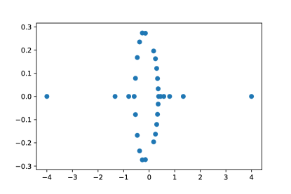
(b) $\mathcal{B}_{m,30}$

(c) $\widetilde{\mathcal{B}}_{m,8}$

(d) $\widetilde{\mathcal{B}}_{m,30}$

Figure 11: configurations of branch points.

In the case of hyperelliptic curves, we compare our timings with the existing Magma code [22]. We obtain a huge speedup which is mostly due to the better integration scheme, but more interesting is the fact that the running time of our algorithm mainly depends on the genus and the precision, while that of Magma depends a lot on the branch points and behaves very badly in terms of the precision.

		bits	128	512	2000	4000	10000
genus	curve	digits	38	154	600	1200	3000
3	$\mathcal{B}_{2,8}$	Arb	5e-3	0.01	0.16	0.48	3.99
		Magma (new)	0.05	0.08	0.44	2.16	25.3
		Magma (old)	0.33	0.44	6.28	421	—
	$\widetilde{\mathcal{B}}_{2,8}$	Arb	5e-3	0.01	0.17	0.54	4.58
		Magma (new)	0.06	0.11	0.67	3.42	40.6
		Magma (old)	0.42	0.45	6.44	457	—
14	$\mathcal{B}_{2,30}$	Arb	0.05	0.22	1.99	8.74	80.9
		Magma (new)	0.55	0.94	4.64	18.7	185.1
		Magma (old)	5.15	10.1	134	9291	—
	$\widetilde{\mathcal{B}}_{2,30}$	Arb	0.05	0.23	2.11	9.31	87.8
		Magma (new)	0.51	1.02	5.40	21.9	227
		Magma (old)	14.8	42.6	370	12099	—
39	$\mathcal{B}_{2,80}$	Arb	0.69	1.64	16.1	70.5	601
		Magma (new)	6.29	9.08	36.4	122	1024

Table 1: timings for hyperelliptic curves, single core Xeon E5 3GHz (in seconds).

		bits	128	512	2000	4000	10000
genus	curve	digits	38	154	600	1200	3000
21	$\mathcal{B}_{7,8}$	Arb	0.06	0.27	4.25	29.5	455
		Magma (new)	0.23	1.06	14.6	83.1	1035
	$\widetilde{\mathcal{B}}_{7,8}$	Arb	0.03	0.19	7.44	58.8	1027
		Magma (new)	0.30	1.64	23.9	132	1613
84	$\mathcal{B}_{25,8}$	Arb	0.09	0.45	8.86	55.6	727
		Magma (new)	0.74	2.60	27.2	135	1529
87	$\mathcal{B}_{7,30}$	Arb	2.05	6.46	43.9	249	3091
		Magma (new)	2.29	10.0	93.8	461	4990
348	$\mathcal{B}_{25,30}$	Arb	2.82	9.57	101	557	6195
		Magma (new)	19.9	41.4	234	1014	9614
946	$\mathcal{B}_{25,80}$	Arb	67.8	182	952	4330
		Magma (new)	369	585	2132	7474

Table 2: timings for superelliptic curves, single core Xeon E5 3GHz (in seconds).

10 Outlook

In this paper we presented an approach based on numerical integration for multiprecision computation of period matrices and the Abel-Jacobi map of superelliptic curves given by $m>1$ and squarefree $f\in\mathbb{C}[x]$.

Integration along a spanning tree and the special geometry of such curves make it possible to compute these objects too high precision performing only a few numerical integrations. The resulting algorithm has an excellent scaling with the genus and works for several thousand digits of precision.

10.1 Reduced small period matrix

For a given curve our algorithm computes a small period matrix $\tau$ in the Siegel upper half-space $\mathcal{H}_{g}$ which is arbitrary in the sense that it depends on the choice of a symplectic basis made during the algorithm.

For applications like the computation of theta functions it is useful to have a small period matrix in the Siegel fundamental domain $\mathcal{F}_{g}\subset\mathcal{H}_{g}$ (see [12, §1.3]).

We did not implement any such reduction. The authors of [12] give a theoretical sketch of an algorithm (Algorithm 1.9) that achieves this reduction step, as well as two practical versions (Algorithms 1.12 and 1.14) which work in any genus and have been implemented for $g\leq 3$. It would be interesting to combine this with our implementation.

10.2 Generalizations

We remark that there is no theoretical obstruction to generalizing our approach to more general curves. In a first step the algorithm could be extended to all complex superelliptic curves given by $m>1$ and $f\in\mathbb{C}[x]$, where $f$ can have multiple roots of order at most $m-1$. Although several adjustments would have to be made (e.g. differentials, homology, integration), staying within the superelliptic setting promises a fast and rigorous extension of our algorithm.

We also believe that the strategy employed here (numerical integration between branch points combined with information about local intersections) could be adapted to completely general algebraic curves given by $F\in\mathbb{C}[x,y]$. However, serious issues have to be overcome:

• On the numerical side we no longer have a nice $m$-th root function, it may be replaced by Newton’s method between branch points (analytic continuation has to be performed on all sheets) and Puiseux series expansion around them.

• On the geometric side we cannot easily define loops, so that given a set of “half” integrals each connecting two branch points, we need to combine them in order to obtain all at once true loops and a symplectic basis. An appropriate notion of shifting number and local intersection is needed here, as well as a combination technique.

We did not investigate further: at this point the advantages of superelliptic curves which are utilized by our approach are already lost (simple geometry of branch points and $m-1$ integrals at the cost of one), so it is not clear whether this approach might be more efficient than other methods.

References

• [1] Milton Abramowitz and Irene A. Stegun. Handbook of mathematical functions with formulas, graphs, and mathematical tables, volume 55 of National Bureau of Standards Applied Mathematics Series. For sale by the Superintendent of Documents, U.S. Government Printing Office, Washington, D.C., 1964.
• [2] Wieb Bosma, John Cannon, and Catherine Playoust. The Magma algebra system. I. The user language. J. Symbolic Comput., 24(3-4):235–265, 1997. Computational algebra and number theory (London, 1993).
• [3] Jean-Benoît Bost and Jean-François Mestre. Moyenne arithmético-géométrique et périodes des courbes de genre $1$ et $2$. Gaz. Math., 1(38):36–64, 1988.
• [4] Richard P. Brent and Paul Zimmermann. Modern computer arithmetic, volume 18 of Cambridge Monographs on Applied and Computational Mathematics. Cambridge University Press, Cambridge, 2011.
• [5] M. M. Chawla and M. K. Jain. Error estimates for Gauss quadrature formulas for analytic functions. Math. Comp., 22:82–90, 1968.
• [6] Edgar Costa, Nicolas Mascot, Jeroen Sijsling, and John Voight. Rigorous computation of the endomorphism ring of a jacobian. arXiv preprint arXiv:1705.09248, 2017.
• [7] John E. Cremona and Thotsaphon Thongjunthug. The complex AGM, periods of elliptic curves over $\mathbb{C}$ and complex elliptic logarithms. J. Number Theory, 133(8):2813–2841, 2013.
• [8] Bernard Deconinck and Mark van Hoeij. Computing Riemann matrices of algebraic curves. Phys. D, 152/153:28–46, 2001. Advances in nonlinear mathematics and science.
• [9] Jörg Frauendiener and Christian Klein. Algebraic curves and riemann surfaces in matlab. In Computational approach to Riemann surfaces, pages 125–162. Springer, 2011.
• [10] Jörg Frauendiener and Christian Klein. Computational approach to hyperelliptic riemann surfaces. Letters in Mathematical Physics, 105(3):379–400, 2015.
• [11] F. Johansson. Arb: a C library for ball arithmetic. ACM Communications in Computer Algebra, 47(4):166–169, 2013.
• [12] Pinar Kilicer, Hugo Labrande, Reynald Lercier, Christophe Ritzenthaler, Jeroen Sijsling, and Marco Streng. Plane quartics over q with complex multiplication. arXiv preprint arXiv:1701.06489, 2017.
• [13] Greg Kuperberg. Kasteleyn cokernels. Electronic Journal of Combinatorics, 9, 2002.
• [14] Hugo Labrande. Explicit computation of the Abel-Jacobi map and its inverse. Theses, Université de Lorraine ; University of Calgary, November 2016.
• [15] The LMFDB Collaboration. The l-functions and modular forms database. http://www.lmfdb.org, 2013. [Online; accessed 16 September 2013].
• [16] Nicolas Mascot. Computing modular Galois representations. Rend. Circ. Mat. Palermo (2), 62(3):451–476, 2013.
• [17] Rick Miranda. Algebraic Curves and Riemann Surfaces (Graduate Studies in Mathematics, Vol 5). American Mathematical Society, 4 1995.
• [18] Pascal Molin. Intégration numérique et calculs de fonctions L. PhD thesis, Université de Bordeaux I, 2010.
• [19] Pascal Molin and Christian Neurohr. hcperiods: arb and magma packages for periods of superelliptic curves. https://doi.org/10.5281/zenodo.833727, July 2017.
• [20] Christopher Towse. Weierstrass points on cyclic covers of the projective line. Transactions of the American Mathematical Society, 348(8):3355–3378, 1996.
• [21] Paul Van Wamelen. Equations for the jacobian of a hyperelliptic curve. Transactions of the American Mathematical Society, 350(8):3083–3106, 1998.
• [22] Paul B. van Wamelen. Computing with the analytic Jacobian of a genus 2 curve. In Discovering mathematics with Magma, volume 19 of Algorithms Comput. Math., pages 117–135. Springer, Berlin, 2006.