Sparse Recovery With Multiple Data Streams: A Sequential Adaptive Testing Approach

Abstract

Multistage design has been used in a wide range of scientific fields. By allocating sensing resources adaptively, one can effectively eliminate null locations and localize signals with a smaller study budget. We formulate a decision-theoretic framework for simultaneous multi-stage adaptive testing and study how to minimize the total number of measurements while meeting pre-specified constraints on both the false positive rate (FPR) and missed discovery rate (MDR). The new procedure, which effectively pools information across individual tests using a simultaneous multistage adaptive ranking and thresholding (SMART) approach, achieves precise error rates control and leads to great savings in total study costs. Numerical studies confirm the effectiveness of SMART for controlling both the FPR and MDR and show that it outperforms existing methods. The SMART procedure is illustrated through the analysis of large-scale A/B tests, high-throughput screening and image analysis.

Keywords: Compound Decision Problem; Distilled Sensing; False Discovery Rate; Missed Discovery Rate; Sequential Probability Ratio Test

1 Introduction

Consider the problem of recovering the support of a high-dimensional vector $\boldsymbol{\mu}=(\mu_{1},\cdots,\mu_{p})\in\mathbb{R}^{p}$ based on measurements from variables $X_{1}$, $\cdots$, $X_{p}$. Let $\mathcal{S}=\{i:\mu_{i}\neq 0\}$ denote the support of $\boldsymbol{\mu}$. We focus on a setup where measurements on variables are performed sequentially and the data obey the following multistage random mixture model (Bashan et al., 2011; Wei and Hero, 2013; Malloy and Nowak, 2014a):

$$X_{ij}\;{\sim}\;(1-\pi)F_{0}+\pi F_{1i};\;i=1,\cdots,p.$$ (1.1)

The measurements are taken in stages $j=1,2,\cdots$, where $X_{ij}$ follow the null distribution $F_{0}$ if $i\notin\mathcal{S}$ and the non-null distribution $F_{1i}$ if $i\in\mathcal{S}$. The model assumes that $F_{0}$ is identical for all $i\notin\mathcal{S}$, whereas $F_{1i}$ can vary across $i\in\mathcal{S}$. Allowing for heterogeneous $F_{1i}$ is desirable in applications where non-zero coordinates have different effect sizes across the $p$ testing units. The mixing proportion $\pi$ is usually small, and can be understood as follows: $X_{i1}$ has probability $1-\pi$ of being a null case and probability $\pi$ of being a signal. Denote $f_{0}$ and $f_{1i}$ the corresponding densities. This article studies the sparse recovery problem, which aims to find a subset that virtually contains all and only signals.

1.1 Non-adaptive vs. adaptive designs

Consider a setting where each measurement is associated with a fixed cost; hence collecting many repeated measurements on all variables are prohibitively expensive in large-scale studies where $p$ is in the order of thousands and even millions.

In applications with a sequential design, it may not be necessary to measure all features at all stages. Let $\mathcal{A}_{j}\subseteq\mathcal{A}_{0}\coloneqq\{1,\cdots,p\}$, $j=1,2,\cdots$, be a monotone sequence of nested sets, with $\mathcal{A}_{j}\subseteq A_{j-1}$ and $\mathcal{A}_{j}$ denoting the set of coordinates on which measurements are performed at stage $j$. Denote $X_{\mathcal{A}_{j}}=(X_{ij}:i\in\mathcal{A}_{j})$ the corresponding collection of observations. In a non-adaptive setting, $X_{ij}$ are sampled at every stage following a pre-fixed policy and each coordinate $i$ is expected to receive the same amount of measurement budget. In an adaptive sampling design, the sampling scheme varies across different coordinates, with the flexibility of adjusting $\mathcal{A}_{j}$ in response to the information collected at previous stages.

The adaptive sampling and inference framework provides a powerful approach to sparse estimation and testing problems. Intuitively, the sensing resources in later stages can be allocated in a more cost-effective way to reflect our updated contextual knowledge during the course of the study; hence greater precision in inference can be achieved with the same study budgets or computational costs. A plethora of powerful multistage testing and estimation procedures have been developed under this flexible framework; some recent developments include the hierarchical testing procedures for pattern recognition (Blanchard and Geman, 2005; Meinshausen et al., 2009; Sun and Wei, 2015), distilled sensing and sequential thresholding methods for sparse detection (Haupt et al., 2011; Malloy and Nowak, 2011, 2014a), multi-scale search and open-loop feedback control algorithms for adaptive estimation (Bashan et al., 2011; Wei and Hero, 2013, 2015) and sequentially designed compressed sensing (Haupt et al., 2012; Malloy and Nowak, 2014b). These works demonstrate that methodologies adopting adaptive designs can substantially outperform those developed under non-adaptive settings.

Our goal is to develop a cost-effective multistage sampling and inference procedure to narrow down the focus in a sequential manner to identify the vector support reliably. The proposed strategy consists of (a) a stopping rule for selecting the active coordinates, and (b) a testing rule for deciding whether a coordinate contains a signal.

1.2 Applications and statistical challenges

Multistage experiments have been widely used in many scientific fields including large-scale A/B testing (Johari et al., 2015), environmental sciences (Cormack, 1988; Thompson and Seber, 1996), microarray, RNA-seq, and protein array experiments (Müller et al., 2004; Rossell and Müller, 2013), geostatistical analysis (Roesch, 1993; Bloma et al., 2002), genome-wide association studies (Satagopan et al., 2004; Rothman et al., 2010) and astronomical surveys (Meinshausen et al., 2009). We first describe some applications and then discuss related statistical issues.

• High-throughput screening [HTS, Zhang et al. (1999); Bleicher et al. (2003)]. HTS is a large-scale hierarchical process that has played a crucial role in fast-advancing fields such as stem cell biology and drug discovery. In drug discovery, HTS involves testing a large number of chemical compounds in multiple stages including target identification, assay development, primary screening, confirmatory screening, and follow-up of hits. The accurate selection of useful compounds is an important issue at each aforementioned stage of HTS. For example, at the primary screening stage, a library of compounds is tested to generate an initial list of active compounds (hits). The goal of this stage is to reduce the size of the library significantly with negligible false negative rate. In the confirmatory screening stage, the hits are further investigated to generate a list of confirmed hits (leads), which will be used to develop drug candidates. As the lab costs for leads generation are very high, an important task at the confirmatory stage is to construct a subset with negligible false positive rate while keeping as many useful compounds as possible.

• Large-scale A/B testing. A/B testing has begun to be widely deployed by various high-tech firms for identifying features/designs that work the best among a large number of potential candidates. It provides a powerful tool for testing new ideas for a wide range of real-world decision-making scenarios. For example, A/B testing can offer key insights on (a) how to improve the users’ experiences, (b) what new features should be incorporated into the product to boost the profits, and (c) which design is the most effective for getting more people click the sign-up button. A significant challenge in large-scale A/B testing is the multiplicity issue, i.e. we need to conduct hundreds of experiments simultaneously for a long period, and each experiment may involve thousands of metrics to be evaluated throughout the entire duration. An effective multistage design can substantially save study costs, minimize risk exposures to customers and enable faster decision making.

• Ultra-high dimensional testing in astronomical surveys. The fast and accurate localization of sparse signals poses a significant challenge in Astrophysics (Meinshausen and Rice, 2006). When a large number of images are taken with high frequencies, the computational cost of an exhaustive search through every single image and pixel can be prohibitively expensive as the search often involves testing billions of hypotheses. A multistage decision process can lead to great savings in total sensing efforts by quickly narrowing down the focus to a much smaller subset of most promising spots in the images (Djorgovski et al., 2012).

These three applications will be discussed in detail in Section 6.

In the design and analysis of large-scale multistage studies, the inflation of decision errors and soaring study costs are among the top concerns. First, to identify useful signals effectively, we need to control the false negative rate to be small at all stages since missed signals will not be revisited in subsequent stages. Second, to reduce the study costs, it is desirable to eliminate as many null locations as possible at each stage. Finally, to avoid misleading scientific conclusions, the final stage of our analysis calls for a strict control of the false positive rate. We aim to develop a simultaneous inference framework for multistage decision process to address the above issues integrally.

1.3 Problem formulation

The sequential sparse recovery problem can be viewed as a compound decision problem (Robbins, 1951), where each component problem involves testing a single hypothesis $H_{0}:\mu=0$ vs. $H_{1}:\mu\neq 0$ based on sequentially collected observations. The basic framework is formulated in the seminal work of Wald (1945), where the following constrained optimization problem is studied:

$$\mbox{ minimize }\mathbb{E}(N)\text{ subject to }\mathbb{P}_{H_{0}}(\mbox{Reject})\leq\alpha^{\prime}\;\mbox{and}\;\mathbb{P}_{H_{1}}(\mbox{Accept})\leq\gamma^{\prime}.$$ (1.2)

Here $N$ is the stopping time, and $\alpha^{\prime}$ and $\gamma^{\prime}$ are pre-specified Type I and Type II error rates. $\mathbb{E}(N)$, which represents the average sampling costs, characterizes the efficiency of a sequential procedure. The sequential probability ratio test (SPRT) is shown to be optimal (Wald, 1945; Siegmund, 1985) for the single sequential testing problem (1.2) in the sense that it has the smallest $\mathbb{E}(N)$ among all sequential procedures at level $(\alpha^{\prime},\gamma^{\prime})$.

When many coordinate-wise sequential decisions are made simultaneously, the control of inflated decision errors becomes a critical issue. Denote $\theta_{i}=\mathbb{I}(\mu_{i}\neq 0)$, where $\mathbb{I}(\cdot)$ is an indicator function. Let $\boldsymbol{\delta}=(\delta_{1},\cdots,\delta_{p})$, where $\delta_{i}=0/1$ indicates that $i$ is classified as a null/non-null case. The true and estimated supports are denoted $\mathcal{S}=(i:\theta_{i}=1)\;\mbox{and}\;\hat{\mathcal{S}}=(i:\delta_{i}=1),$ respectively. Define the false positive rate (FPR) and missed discovery rate (MDR) as

$$\mbox{FPR}({\boldsymbol{\delta}})=\frac{\mathbb{E}\{\sum_{i=1}^{p}(1-\theta_{i})\delta_{i}\}}{\mathbb{E}(\sum_{i=1}^{p}\delta_{i})}\;\mbox{ and }\;\mbox{MDR}({\boldsymbol{\delta}})=\frac{\mathbb{E}\left\{\sum_{i=1}^{p}\theta_{i}(1-\delta_{i})\right\}}{\mathbb{E}(\sum_{i=1}^{p}\theta_{i})}.$$ (1.3)

Remark 1.

The FPR is also referred to as the marginal false discovery rate (mFDR; Genovese and Wasserman, 2002; Sun and Cai, 2007). In the non-sequential setting, the FPR and the widely used false discovery rate (FDR; Benjamini and Hochberg, 1995) are shown to be asymptotically equivalent for the Benjamini-Hochberg procedure (Genovese and Wasserman, 2002) and a general class of FDR procedures (Proposition 7 in Appendix A.2 in Cai et al. (2019)). Such asymptotic equivalence requires further research under the sequential setting. The main consideration of using FPR (as opposed to FDR) is to develop optimality results under a decision-theoretic framework (Berger, 1985). Theorem 3 shows that our proposed method controls both the FPR and FDR. An alternative measure to the MDR is the false negative rate (FNR; Genovese and Wasserman, 2002; Sarkar, 2004). The concepts of FNR and MDR are different, with the MDR being a more appropriate error measure in the sparse setting; see Meinshausen and Rice (2006); Haupt et al. (2011); Cai and Sun (2017) for related discussions.

To evaluate the efficiency of a multistage testing method, we use the expected sample size (ESS) per unit

$$\mbox{ESS}(\boldsymbol{N})=\mathbb{E}\left(p^{-1}\textstyle\sum_{i=1}^{p}N_{i}\right),$$ (1.4)

where $\boldsymbol{N}=(N_{1},\cdots,N_{p})$, with $N_{i}$ being the sample size, or stopping time in Berger (1985) and Siegmund (1985), at coordinate $i$. Let $\alpha$ and $\gamma$ be the pre-specified FPR and MDR levels. We study the following constrained optimization problem:

$$\mbox{ minimize }\mbox{ESS}(\boldsymbol{N})\text{ subject to }\mbox{FPR}(\boldsymbol{\delta})\leq\alpha\;\mbox{and}\;\mbox{MDR}(\boldsymbol{\delta})\leq\gamma.$$ (1.5)

The formulation (1.5) naturally extends the classical formulation (1.2) in Wald (1945) and Siegmund (1985) to the compound decision setting.

1.4 Main contributions

The error control in multi-stage testing has been studied extensively, e.g. in Benjamini and Heller (2007); Victor and Hommel (2007); Dmitrienko et al. (2007); Goeman and Mansmann (2008); Yekutieli (2008); Liang and Nettleton (2010); Benjamini and Bogomolov (2014). However, existing methods are usually designed for different types of applications and cannot be easily tailored for the problem under consideration. The biggest limitation is that existing works only focus on the control of false positive errors. Moreover, the ranking and stopping rules developed in Zehetmayer et al. (2008); Posch et al. (2009); Sarkar et al. (2013) are suboptimal because data combination procedures based on $p$-values do not fully utilize data from different stages and fail to exploit the overall structure of the compound decision problem. Recent works on sequential testing based on SPRT rules (Bartroff and Song, 2013; Bartroff, 2014; Bartroff and Song, 2016) are computationally intensive, making it infeasible for large-scale studies such as those arising from HTS and Astrophysics where millions of tests are conducted simultaneously. Finally, the optimality issue has not been addressed by the above mentioned works.

We formulate the sparse recovery problem as a sequential testing problem with multiple data streams. A new adaptive testing procedure is developed under the compound decision-theoretic framework. The proposed procedure, which employs a simultaneous multistage adaptive ranking and thresholding (SMART) approach, not only utilizes all information collected through multiple stages but also exploits the compound structure of the decision problem to pool information across different coordinates. We show that SMART controls the FPR and MDR and achieves the information-theoretic lower bounds. SMART is simple, fast, and capable of dealing with millions of tests. Numerical studies confirm the effectiveness of SMART for error rates control and demonstrate that it leads to substantial savings in study costs.

SMART has several advantages over existing methods for sparse recovery such as distilled sensing (DS, Haupt et al. (2011)) and simple sequential thresholding (SST, Malloy and Nowak (2014a)). First, DS and SST use fixed thresholding rules that do not offer accurate error rate control. Second, although DS and SST employ a multistage design, the stopping and testing rules at stage $k$ only depend on the observations at the current stage, and the observations from previous stages are abandoned. Finally, as opposed to DS and SST that ignore the compound decision structure, SMART employs the ranking and compound thresholding idea in the multiple testing literature (Sun and Cai, 2007) to pool information across individual tests. Consequently, SMART controls the error rates more precisely with substantial efficiency gain.

1.5 Organization of the paper

In Section 2 we first formulate a compound decision-theoretic framework for sequential sparse recovery problems, and then develop oracle rules for FPR and MDR control. Section 3 proposes the SMART procedure and discusses its implementation. Section 4 derives the fundamental limits for sparse inference and establishes the asymptotic optimality of SMART. In Section 5, we conduct numerical experiments to compare SMART with competitive methods. Section 6 applies SMART for analyzing data from large-scale A/B testing, high-throughput screening and astronomical surveys. The proofs, technical derivations and additional numerical results are provided in the Supplementary Material.

2 Oracle Rules for Sparse Recovery

The sparse recovery problem in the adaptive setting involves the simultaneous testing of $p$ hypotheses:

$$H_{0,i}:\mu_{i}=0\mbox{ vs. }H_{1,i}:\mu_{i}\neq 0,\quad 1\leq i\leq p,$$ (2.1)

based on $p$ streams of observations $\{(X_{i1},X_{i2},\cdots):1\leq i\leq p\}$. In this section, we first formulate the sequential sparse recovery problem in a decision-theoretic framework (Section 2.1), then derive an oracle procedure for FPR and MDR control (Section 2.2), and finally propose strategies to approximate the oracle procedure (Sections 2.3-2.4).

2.1 A decision-theoretic formulation

Let $X_{ij}$ be the measurement of variable $X_{i}$ at stage $j$ and $\boldsymbol{X}_{i}^{j}=(X_{i1},\cdots,X_{ij})$ the collection of measurements on $X_{i}$ up to stage $j$. A multistage decision procedure involves choosing a stopping rule and a testing rule for each location. At location $i$, the stopping rule $\boldsymbol{\tau}_{i}$ consists of a series of functions $\tau_{i1}(\boldsymbol{X}_{i}^{1})$, $\tau_{i2}(\boldsymbol{X}_{i}^{2})$, $\cdots$, where $\tau_{ij}$ takes values in $\{0,1\}$, with 0 and 1 standing for “taking another observation” and “stopping sampling and making a decision”, respectively. We consider a class of multistage designs where the focus is sequentially narrowed down, i.e. the active sets satisfy $\mathcal{A}_{1}=\{1,\cdots,p\}$, and $\mathcal{A}_{j}\subseteq\mathcal{A}_{j-1}$ for $j=2,3,\cdots$. At every coordinate $i\in\mathcal{A}_{j}$, there are three possible actions: (i) stop sampling and claim $H_{0,i}$ is true; (ii) stop sampling and claim $H_{0,i}$ is false; and (iii) do not make a decision and take another observation. We first focus on the case where one sample is collected per stage; the case with multiple samples is discussed in Section 3.3.

We follow the standard notations under the decision-theoretic framework detailed in Chp. 7 of Berger (1985). The stopping rule $\boldsymbol{\tau}_{i}$ can be equivalently described by the stopping time $N_{i}=\min\{n\geq 1:\tau_{in}(\boldsymbol{X}_{i}^{n})=1\}$, the final stage at which we stop sampling and make a decision. If we collect one sample per stage, we use the terms sample size and stopping time interchangeably. The testing rule $\delta_{i}\in\{0,1\}$ is carried out at the terminal sampling stage $N_{i}$, where $\delta_{i}=0$ (1) indicates that coordinate $i$ is classified as a null (non-null) case. A multistage decision procedure is therefore denoted $\boldsymbol{d}=(\boldsymbol{N},\boldsymbol{\delta})$, where $\boldsymbol{N}=(N_{1},\cdots,N_{p})$ and $\boldsymbol{\delta}=(\delta_{1},\cdots,\delta_{p})$ are sample sizes and terminal decisions, respectively.

Assume that the cost of taking one observation is $c$. From a decision-theoretic viewpoint, we can study a weighted classification problem with the loss function:

$$L_{\lambda_{1},\lambda_{2}}(\boldsymbol{\theta},\boldsymbol{d})=\textstyle\lambda_{1}\left\{\sum_{i=1}^{p}(1-\theta_{i})\delta_{i}\right\}+\lambda_{2}\left\{\sum_{i=1}^{p}\theta_{i}(1-\delta_{i})\right\}+c\sum_{i=1}^{p}N_{i},$$ (2.2)

where $\lambda_{1}$ and $\lambda_{2}$ are the costs for a false positive decision and a false negative decision, respectively. The sum of the first two terms in (2.2) corresponds to the total decision errors, and the last term gives the total sampling costs. The optimal solution to the weighted classification problem is the Bayes sequential procedure $\boldsymbol{d}^{\pi}$ that minimizes the expected loss

$$E\{L_{\lambda_{1},\lambda_{2}}(\boldsymbol{\theta},\boldsymbol{d}^{\pi})\}=\textstyle\inf_{\boldsymbol{d}}E\{L_{\lambda_{1},\lambda_{2}}(\boldsymbol{\theta},\boldsymbol{d})\}.$$ (2.3)

In Berger (1985), $\boldsymbol{d}^{\pi}$ is represented by a thresholding rule based on the oracle statistic

$$T_{OR}^{i,j}=\mathbb{P}(\theta_{i}=0|\boldsymbol{X}_{i}^{j}).$$ (2.4)

$T_{OR}^{i,j}$ is the posterior probability of case $i$ being a null given $\boldsymbol{X}_{i}^{j}$. We view $T_{OR}^{i,j}$ as a significance index reflecting our confidence on claiming that $H_{0,i}$ is true based on all information available at stage $j$.

In practice we only specify the FPR and MDR levels $\alpha$ and $\gamma$ but do not know $\lambda_{1}$ and $\lambda_{2}$. However, the optimal solution to the weighted classification problem (2.3) motivates us to conjecture that the optimal solution to the sparse recovery problem (1.5) should also be a thresholding rule based on $T_{OR}^{i,j}$. This conjecture is established rigorously in Theorem 1 of the next subsection.

2.2 Oracle procedure

Let $t_{l}$ and $t_{u}$ be constants satisfying $0<t_{l}<t_{u}<1$. Consider a class of sequential testing procedures $\boldsymbol{d}^{\pi}(t_{l},t_{u})$ of the form:

$$\mbox{ stop sampling for unit $i$ at }N_{i}=\min\{j\geq 1:T_{OR}^{i,j}\leq t_{l}\;\mbox{or}\;T_{OR}^{i,j}\geq t_{u}\},$$

and decide $$\delta_{i}=1 T_{OR}^{i,j}\leq t_{l} \delta_{i}=0 T_{OR}^{i,j}\geq t_{u}$$ if and if . (2.5)

Denote by $\mathcal{D}_{\alpha,\gamma}$ the collection of all sequential decision procedures which simultaneously satisfy $(i)\;\mbox{FPR}({\boldsymbol{d}})\leq\alpha\;\mbox{and}\;(ii)\;\mbox{MDR}({\boldsymbol{d}})\leq\gamma.$ The following assumption, which is a standard condition in the sequential analysis literature (cf. Berger, 1985; Siegmund, 1985), requires that $f(\boldsymbol{X}_{i}^{1}|\theta_{i}=0)$ and $f(\boldsymbol{X}_{i}^{1}|\theta_{i}=1)$ differ with some positive probability. This ensures that the sequential testing procedure will stop within a finite number of stages.

Assumption 1.

$\mathbb{P}_{\theta_{i}}\left(\log\left\{\frac{f\left(\boldsymbol{X}_{i}^{1}|\theta_{i}=1\right)}{f\left(\boldsymbol{X}_{i}^{1}|\theta_{i}=0\right)}\right\}=0\right)<1$ for $i=1,\cdots,p$.

The next theorem derives an oracle sequential testing procedure that provides the optimal solution to the constrained optimization problem (1.5).

Theorem 1.

Consider a class of sequential testing rules $\boldsymbol{d}^{\pi}(t_{l},t_{u})$ taking the form of (2.2). Denote $Q_{OR}(t_{l},t_{u})$ and $\tilde{Q}_{OR}(t_{l},t_{u})$ the FPR and MDR levels of $\boldsymbol{d}^{\pi}(t_{l},t_{u})$, respectively. Then under Assumption 1, we have

(a). $Q_{OR}(t_{l},t_{u})$ is non-decreasing in $t_{l}$ for a fixed $t_{u}$, and $\tilde{Q}_{OR}(t_{l},t_{u})$ is non-increasing in $t_{u}$ for a fixed $t_{l}$.

(b). Let $0<\alpha,\gamma<1$. Then there exists a pair of oracle thresholds $(t_{OR}^{l},t_{OR}^{u})$, based on which we can define the oracle procedure

$$\boldsymbol{d}_{OR}\equiv\boldsymbol{d}^{\pi}(t_{OR}^{l},t_{OR}^{u})$$ (2.6)

such that $\boldsymbol{d}_{OR}$ is optimal in the sense that (i) $\mbox{FPR}({\boldsymbol{d}_{OR}})\leq\alpha$; (ii) $\mbox{MDR}({\boldsymbol{d}_{OR}})\leq\gamma$; and (iii) $\mbox{ESS}({\boldsymbol{d}_{OR}})\leq\mbox{ESS}({\boldsymbol{d}_{*}})$ for all $\boldsymbol{d}_{*}\in\mathcal{D}_{\alpha,\gamma}$.

Remark 2.

The development of a multiple testing procedure consists of two steps: deriving the optimal ranking statistic and finding a threshold along the ranking. Under the FPR criterion, the optimal ranking statistic is $T_{OR}$. The recent work by Heller and Rosset (2019) indicates that $T_{OR}$ is also optimal under the FDR criterion. The FPR criterion leads to fixed thresholds $t_{OR}^{l}$ and $t_{OR}^{u}$. By contrast, the theory in Heller and Rosset (2019) indicates that the thresholds must be functions of data when the FDR criterion is used. It is important to note that the oracle rule is only used to motivate our methodology in later sections. Algorithm 1 in Section 3.1 controls both the FDR and FPR, and employs data-driven thresholds that vary across data sets. More comparisons and discussions of the FDR and FPR criteria are provided in Heller and Rosset (2019) and Appendix D of the Supplementary Material.

The oracle procedure $\boldsymbol{d}_{OR}$ is a thresholding rule based on the oracle statistic $T_{OR}$ and oracle thresholds $t_{OR}^{l}$ and $t_{OR}^{u}$. However, Theorem 1 only shows the existence of $t_{OR}^{l}$ and $t_{OR}^{u}$, which are unknown in practice. In Section 2.3, we extend the classical ideas in Wald (1945) and Siegmund (1985) to derive approximations of $t_{OR}^{l}$ and $t_{OR}^{u}$.

2.3 Approximation of oracle thresholds and its properties

If we focus on a single location $i$, then the sequential probability ratio test (SPRT) (Wald, 1945) is a thresholding rule based on $\mathcal{L}_{i,j}=\frac{f(\boldsymbol{X}_{i}^{j}|\theta_{i}=1)}{f(\boldsymbol{X}_{i}^{j}|\theta_{i}=0)}$ and of the form

$$\begin{array}[]{lll}\mbox{if $\log\mathcal{L}_{i,j}\leq a$},&\mbox{stop sampling and decide $H_{0,i}$ is true;}\\ \mbox{if $\log\mathcal{L}_{i,j}\geq b$,}&\mbox{stop sampling and decide $H_{0,i}$ is false;}\\ \mbox{if $a<\log\mathcal{L}_{i,j}<b$,}&\mbox{take another observation.}\end{array}$$

Let $\alpha^{\prime}=\mathbb{P}_{H_{0,i}}(\mbox{Reject $H_{0,i}$})$ and $\gamma^{\prime}=\mathbb{P}_{H_{1,i}}(\mbox{Accept $H_{0,i}$})$ be prespecified Type I and Type II error rates. Then by applying Wald’s identify, the thresholds $a$ and $b$ can be approximated as:

$$\tilde{a}=\log\frac{\gamma^{\prime}}{1-\alpha^{\prime}}\;\mbox{ and }\;\tilde{b}=\log\frac{1-\gamma^{\prime}}{\alpha^{\prime}}.$$ (2.7)

The oracle statistic $T_{OR}^{i,j}=(1-\pi)/\{(1-\pi)+\pi\mathcal{L}_{i,j}\}$ is monotone in $\mathcal{L}_{i,j}$. Therefore in the multiple hypothesis setting, we can view the oracle rule $\boldsymbol{d}_{OR}=\boldsymbol{d}^{\pi}(t_{OR}^{l},t_{OR}^{u})$ as $m$ parallel SPRTs. Then the problem boils down to how to obtain approximate formulas of the oracle thresholds $t_{OR}^{l}$ and $t_{OR}^{u}$ for a given pair of pre-specified FPR and MDR levels $(\alpha,\gamma)$. In our derivation, the classical techniques (e.g. Section 7.5.2 in Berger (1985)) are used, and the relationships between the FPR and MDR levels $(\alpha,\gamma)$ and the Type I and Type II error rates $(\alpha^{\prime},\gamma^{\prime})$ are exploited. The derivation of approximation formulas with the FPR and MDR constraints is complicated; we provide the key steps in Section B of the Supplementary Material. The approximated thresholds are given by

$$\tilde{t}_{OR}^{l}=\alpha\;\mbox{ and }\;\tilde{t}_{OR}^{u}=\frac{1-\pi}{\pi\gamma+1-\pi}.$$ (2.8)

The next theorem shows that the pair (2.8) is valid for FPR and MDR control.

Theorem 2.

Consider multistage model (1.1). Denote $\tilde{\boldsymbol{d}}_{OR}=\boldsymbol{d}^{\pi}(\tilde{t}_{OR}^{l},\tilde{t}_{OR}^{u})$ the thresholding procedure that operates according to (2.2) with upper and lower thresholds given by (2.8). Then we have

$$\mbox{FPR}(\tilde{\boldsymbol{d}}_{OR})\leq\alpha \mbox{FDR}(\tilde{\boldsymbol{d}}_{OR})\leq\alpha \mbox{MDR}(\tilde{\boldsymbol{d}}_{OR})\leq\gamma.$$, and

2.4 Accuracy of approximations

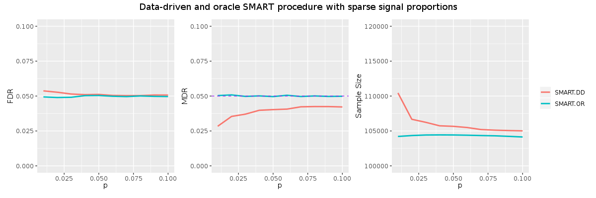
Figure 1: Error rates and total samples for data-driven and oracle SMART procedures with varying sparse signal proportions.

The approximations in (2.8) lead to very conservative FPR and MDR levels. The main issue is the “overshooting” phenomenon that we shall explain next. The SPRT process $\{\log\mathcal{L}_{ij}:j=1,2,\cdots\}$ can be roughly conceptualized as a Brownian motion (e.g. Chp 3, Siegmund (1985)) with average “step size” given by $E_{\theta_{i}}[\log\{f_{1}(X_{ik})/f_{0}(X_{ik})\}]$. Figure 1 gives the sample paths, for units with large and small step sizes respectively, to illustrate how the SPRT statistics evolve under the null and alternative. The SPRT makes a decision when $\log\mathcal{L}_{ij}$ leaves the interval $(a,b)$.

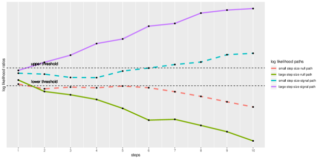
Figure 1: The sample paths for two SPRTs, with the null being $N(0,1)$, and alternative being $N(1,1)$ (dashed lines, smalle steps) and $N(2,1)$ (solid lines, large steps), respectively. $L_{ij}$ change drastically with large steps, accentuating the overshooting issue.

The derivation of $\tilde{t}_{OR}^{l}$ and $\tilde{t}_{OR}^{u}$ involves the application of Wald’s approximation, under the assumption that the two boundaries are hit exactly by $\log\mathcal{L}_{ij}$. However, in practice the assumption is highly idealized as shown by the sample paths in Figure 1; this is referred to as “overshooting” (Section 7.5.3, Berger (1985)). Theorem 12 in Section 7.5.3 of Berger (1985) indicates that “overshooting” tends to overestimate the true error probabilities and lead to conservative error control. Our simulation shows that the FPR of the SPRTs based on Wald’s approximations can be as low as 0.01 when the nominal FPR level is 0.05. The conservativeness in the error rates control would result in loss of efficiency. The situation is much exacerbated in high-dimensional settings where most locations are only tested once or twice (i.e. the SPRTs have “large step sizes”). The above concern motivates us to develop new methodologies in the next section.

3 Sparse Recovery via SMART

The oracle procedure $\boldsymbol{d}_{OR}$ (2.6) provides the optimal solution to the sparse recovery problem. It can be interpreted in two ways: one is a collection of $p$ parallel and independent SPRTs, and the other is a stage-wise simultaneous inference procedure. This section takes the latter view. To gain more insights on the overall structure of the problem, we rewrite (2.2) as the sum of stage-wise losses:

$$L_{\lambda_{1},\lambda_{2}}(\boldsymbol{\theta},\boldsymbol{d})=\sum_{j=1}^{N}\left[\sum_{i\in\mathcal{S}_{j}}\left\{\lambda_{1}(1-\theta_{i})\delta_{i}+\lambda_{2}\theta_{i}(1-\delta_{i})\right\}+c\cdot\mbox{Card}(\mathcal{A}_{j})\right],$$ (3.1)

where $N=\max\{N_{i}:1\leq i\leq p\}$ and $\mathcal{S}_{j}=\{i:N_{i}=j\}$. At stage $j$, we stop sampling on $\mathcal{S}_{j}\subset\mathcal{A}_{j}$ and make terminal decisions at every $i\in\mathcal{S}_{j}$; the remaining locations will become the active set for the next stage $\mathcal{A}_{j+1}=\mathcal{A}_{j}\setminus\mathcal{S}_{j}$, on which new observations are taken. We then proceed to make further decisions on $\mathcal{A}_{j+1}$. The process will be repeated until the active set becomes empty.

This simultaneous decision view motivates us to employ the idea of ranking and thresholding that has been widely used in the multiple testing literature. For example, the Benjamini-Hochberg procedure (Benjamini and Hochberg, 1995) first orders all $p$-values from the smallest to largest, and then uses a step-up method to choose a cutoff along the $p$-value ranking. Under (3.1), we make three types of decisions simultaneously at each stage based on ordered $T_{OR}$: (i) identifying non-null cases, (ii) eliminating null cases, and (iii) selecting coordinates for further measurements. The next subsection describes an algorithm that involves simultaneous multistage adaptive ranking and thresholding (SMART).

3.1 The SMART algorithm

The operation of SMART can be described as follows. At stage $j$, we first calculate the oracle statistics in the active set $\mathcal{A}_{j}$ and sort them from smallest to largest. Then we carry out two thresholding procedures along the ranking: part (a) chooses a lower cutoff $\hat{t}_{OR}^{l,j}$ with selected locations claimed as signals; part (b) chooses an upper cutoff $\hat{t}_{OR}^{u,j}$ with selected locations claimed as nulls. We stop sampling on locations where definitive decisions are made, and take new observations on remaining locations for further investigation. The above steps will be iterated until convergence. The detailed operation is described in Algorithm 1.

Algorithm 1. The SMART procedure

Define the lower and upper thresholds $\tilde{t}_{OR}^{l}=\alpha$ and $\tilde{t}_{OR}^{u}=\frac{1-\pi}{\pi\gamma+1-\pi}$.

Let $\mathcal{A}_{j}$ be the active set at stage $j$, $j=1,2,\cdots$.

Iterate Step 1 to Step 3 until $\mathcal{A}_{j}=\emptyset$.

Step 1 (Ranking). For all $i\in\mathcal{A}_{j}$, compute $T_{OR}^{i,j}$ and sort them in ascending order

$T_{OR}^{(1),j}\leq T_{OR}^{(2),j}\leq\cdots\leq T_{OR}^{(k_{j}),j},$ where $k_{j}=\text{Card}(\mathcal{A}_{j})$.

Step 2 (Thresholding).

(a) (Signal discovery). Let $k_{j}^{s}=\max\{r:r^{-1}\sum_{i=1}^{r}T_{OR}^{(i),j}\leq\tilde{t}_{OR}^{l}\}$ and $\hat{t}_{OR}^{l,j}=T_{OR}^{(k_{j}^{s}),j}$.

Define $\mathcal{S}_{j}^{s}=\{i\in\mathcal{A}_{j}:T_{OR}^{i,j}\leq\hat{t}_{OR}^{l,j}\}$. For all $i\in\mathcal{S}_{j}^{s}$, stop sampling and let $\delta_{i}=1$.

(b) (Noise elimination). Let $k_{j}^{e}=\max\{r:r^{-1}\sum_{i=0}^{r-1}(T_{OR}^{(k_{j}-i),j})\geq\tilde{t}_{OR}^{u}\}$

and $\hat{t}_{OR}^{u,j}=T_{OR}^{(k_{j}-k_{j}^{e}+1),j}$. Define $\mathcal{S}_{j}^{e}=\{i\in\mathcal{A}_{j}:T_{OR}^{i,j}\geq\hat{t}_{OR}^{u,j}\}$.

For all $i\in\mathcal{S}_{j}^{e}$, stop sampling and let $\delta_{i}=0$.

Step 3 (Updating). Let $\mathcal{A}_{j+1}=\mathcal{A}_{j}\setminus(\mathcal{S}_{j}^{s}\cup\mathcal{S}_{j}^{e})$. Take new observations on $\mathcal{A}_{j+1}$.

The SMART algorithm utilizes stage-wise thresholds $\hat{t}_{OR}^{l,j}$ and $\hat{t}_{OR}^{u,j}$. The operation of the algorithm implies that we always have $\hat{t}_{OR}^{l,j}\geq\tilde{t}_{OR}^{l}$ and $\hat{t}_{OR}^{u,j}\leq\tilde{t}_{OR}^{l}$ for all $j$. Hence SMART always uses fewer samples than $\tilde{\boldsymbol{d}}_{OR}$. The next theorem shows that SMART is valid for FPR and MDR control.

Theorem 3.

Denote $\boldsymbol{d}_{SM}$ the SMART procedure described in Algorithm 1 with pre-specified FPR and MDR levels $(\alpha,\gamma)$. Then

$${\rm FPR}({\boldsymbol{d}_{SM}})\leq\alpha,\;\rm FDR({\boldsymbol{d}_{SM}})\leq\alpha\;\mbox{ and }\;{\rm MDR}(\boldsymbol{d}_{SM})\leq\gamma.$$

Remark 3.

The FPR and MDR control would not suffer from selection effects. First, the operation of SMART implies that only one terminal decision is made for each coordinate (with no further inference); the action of “collecting one more observation” is an indecision that does not play a role in the FPR or MDR analyses. Second, the theory on FPR and MDR control can be proven under the framework of multiple testing with groups (Efron, 2008; Cai and Sun, 2009) by viewing stages as groups [cf. Section A.3 in the Supplementary Material].

3.2 Overshooting, compound thresholding and knapsack problems

In the thresholding step, SMART chooses the lower and upper cutoffs based on the moving averages of the selected oracle statistics. We call SMART a compound thresholding procedure, for its stage-wise cutoffs $\hat{t}_{OR}^{l,j}$ and $\hat{t}_{OR}^{u,j}$ are jointly determined by data from multiple locations. By contrast, we call $\tilde{\boldsymbol{d}}_{OR}$ a simple thresholding rule as the decision at location $i$ only depends on its own data. By adopting a compound thresholding scheme and pooling information across parallel SPRTs, SMART overcomes the overshoot problem of individual SPRTs. To illustrate the point, consider the following toy example.

Example 3.1.

Let the FDR level $\alpha=0.05$. Suppose at stage $j$ the ordered $T_{OR}$ values are $\{0.01,0.055,0.07,0.10,\cdots\}$. If we use the simple thresholding rule $\tilde{\boldsymbol{d}}_{OR}$ with $\tilde{t}_{OR}^{l}=\alpha=0.05$, then we can reject one hypothesis with $T_{OR}^{(1),j}=0.01$; the gap between $T_{OR}^{(1),j}$ and $\alpha$ is 0.04. By contrast, the moving average of the top three statistics is $0.045<\alpha$; hence SMART rejects three hypotheses. The gap between the moving average and the threshold is only 0.005. Thus the boundary $\alpha$ can be approximately more precisely by the moving average. In large-scale testing problems, the gap is almost negligible, implying very accurate error rate control; this has been corroborated by our simulation studies.

We provide further insights by viewing the decision process of SMART as a 0-1 knapsack problem with varying FPR capacities. Let $k_{j}^{*}=\max\{1\leq i\leq m:T_{OR}^{(i),j}\leq\alpha\}$. Then the discovery step in Algorithm 1 can be written as

$$\textstyle\sum_{i=k_{j}^{*}+1}^{k_{j}^{s}}\left(T_{OR}^{(i),j}-\alpha\right)\leq\sum_{i=1}^{k_{j}^{*}}\left(\alpha-T_{OR}^{(i),j}\right).$$ (3.2)

If we view the nominal FDR level $\alpha$ as the initial capacity in a knapsack problem, then Equation 3.2 shows that every time we reject a hypothesis with $T_{OR}^{i,j}<\alpha$, we will increase the capacity of the knapsack, enabling one to reject hypotheses with $T_{OR}^{i,j}>\alpha$. Hence the approximation errors (overshooting) can be effectively mitigated by aggregating the gaps between $T_{OR}$ and $\alpha$ to increase the capacity and make more discoveries.

3.3 Implementation of SMART

In practice the oracle statistic $T_{OR}$ is unknown and needs to be estimated from data. We present detailed formulae for computing $T_{OR}$ in a Bayesian hierarchical model considered in Bashan et al. (2011); Wei and Hero (2013). The model provides a flexible framework for a range of estimation and testing problems and has been widely used in signal processing. It seems to be in particular suitable for the simultaneous sequential testing problem as it utilizes non-informative priors and allows varied signal magnitudes across locations.

Let $\theta_{1},\cdots,\theta_{p}$ be independent Bernoulli$(\pi)$ variables. Assume that observations $X_{ij}$ obey the following multistage model:

$$X_{ij}=\mu_{i}+\epsilon_{ij},\quad\epsilon_{ij}\sim N(0,\sigma^{2}),$$ (3.3)

where $\mu_{i}=0$ if $\theta_{i}=0$, and $\mu_{i}\sim N\left(\eta_{i},\tau_{i}^{2}\right)$ if $\theta_{i}=1$. Let $\phi(\cdot;\mu,\sigma^{2})$ denote the density of $N(\mu,\sigma^{2})$. At stage $j=1$, $T_{OR}^{i,1}=(1-\pi)\phi(x_{i1};0,\sigma^{2})/f(x_{i1})$ is the local false discovery rate (Lfdr) Efron et al. (2001), which can be estimated well from data without assuming a known alternative as done in Sun and Cai (2007). Specifically, we use Jin-Cai’s method Jin and Cai (2007) to get an initial estimate of ${\pi}$ and ${\sigma}^{2}$, denoted $\hat{\pi}$ and $\hat{\sigma}^{2}$, and then obtain marginal density $f(x_{i1})$ using standard kernel methods. In later stages $j=2,3,\cdots$, we sequentially update $T_{OR}^{i,j}$ using a recursive formula that is described in Section C of the Appendix. Our estimator for the signal magnitude is constructed as a James-Stein type linear shrinkage estimator (James and Stein, 1961), which does not assume that $\eta_{i}$ is known a priori. The shrinkage estimator not only stabilizes the performance of the algorithm but also effectively borrows strength from observations collected at different stages.

Section C in the Supplementary Material also discusses modified computational algorithms for the case with multiple samples per stage. If the number of samples are prefixed, then SMART operates essentially in the same way, except that $T_{OR}^{i,j}$ is calculated based on a modified model

$$X_{ij}=\mu_{i}+\epsilon_{ij},\;\epsilon_{ij}\sim N(0,\sigma^{2}/\kappa_{ij}),$$

with $\kappa_{ij}$ denoting the corresponding number of samples collected. The theory on FPR and MDR control still holds. However, the problem becomes complicated when the number of samples is allowed to be data-driven. Hence the optimal policy must be cast as a dynamic programming problem. We conjecture that the open-loop feedback control (OLFC) algorithm (Wei and Hero, 2013) may be incorporated into SMART but more research is needed. However, there are two complications. First, OLFC aims to optimize the estimation accuracy, whereas we aim to minimize the total sensing efforts subject to the constraints on the FPR and MDR. Second, OLFC can only handle two-stage designs and the extension to more stages is non-trivial.

3.4 Connections to distilled sensing

The distilled sensing (DS, Haupt et al. (2011)) and single sequential thresholding (SST, Malloy and Nowak (2014a)) methods provide efficient adaptive sampling schemes for sparse recovery. SMART employs a similar adaptive sampling and inference framework but improves DS and SST in several ways. First, as opposed to DS and SST that use fixed thresholding rules at all units and through all stages [e.g. DS always uses 0 as the threshold and hence eliminates roughly half of the coordinates in each distillation stage], SMART uses data-driven thresholds that are adaptive to both data and pre-specified FPR and MDR levels. Second, the sampling and inference rules in DS and SST only utilize observations at the current stage. By contrast, the building block of SMART is $T_{OR}^{i,j}$, which utilizes all observations collected up to the current stage. This can greatly increase the signal to noise ratio and lead to more powerful testing and stopping rules. Third, SMART utilizes compound thresholding to exploit the multiple hypothesis structure, which can greatly improve the accuracy of the error rates control. Finally, DS and SST only have a stopping rule to eliminate null locations. Intuitively, such a scheme is inefficient as one should also stop sampling at locations where the evidence against the null is extremely strong. The proposed scheme in Step 2 of SMART involves two algorithms that can simultaneously identify signals and eliminate noise. In other words, SMART stops sampling once a definitive decision ($\delta_{i}=0$ or $\delta_{i}=1$) is reached; this more flexible operation is desirable and would further save study budgets.

4 Limits of Sparse Recovery

This section discusses the notion of fundamental limits in sparse inference for both fixed and adaptive settings. The discussion serves two purposes. First, as the limits reflect the difficulties of support recovery under different settings, they demonstrate the advantage of using adaptive designs over fixed designs. Second, the limit provides an optimality benchmark for what can be achieved asymptotically by any inference procedure in the form of a lower bound; hence we can establish the optimality of an inference procedure by proving its capability of achieving the limit.

4.1 The fundamental limits in adaptive designs

Different from previous sections that consider a finite (and fixed) dimension $p$, the asymptotic analysis in this section assumes that $p\rightarrow\infty$. Under this asymptotic framework, the FPR and MDR levels are denoted $\alpha_{p}$ and $\gamma_{p}$, both of which tend to zero as $p\rightarrow\infty$. In Malloy and Nowak (2014a), the fundamental limits for reliable recovery were established under the family wise error rate (FWER) criterion. This section extends their theory to the important FPR and MDR paradigm.

The basic setup assumes that the null and alternative distributions $F_{0}$ and $F_{1}$ are identical across all locations. This more restrictive model is only for theoretical analysis and our proposed SMART procedure works under the more general model (1.1), which allows $F_{1i}$ to vary across testing units. Let $G$ and $H$ be two distributions with corresponding densities $g$ and $h$. Define $D(G\|H)=\int_{-\infty}^{\infty}g(x)\log{\frac{g(x)}{h(x)}}dx$. Then the Kullback-Leibler (KL) divergence, given by

$$D_{KL}(F_{0},F_{1})=\max\{D(F_{0}\|F_{1}),D(F_{1}\|F_{0})\},$$

can be used to measure the distance between $F_{0}$ and $F_{1}$. Let $\tau$ be the average number of measurements allocated to each unit. Consider a general multistage decision procedure $\boldsymbol{d}$. The performance of $\boldsymbol{d}$ is characterized by its total risk $R^{*}(\boldsymbol{d})=\text{FPR}(\boldsymbol{d})+\text{MDR}(\boldsymbol{d})$. Intuitively, $D_{KL}(F_{0},F_{1})$ and $\tau$ together would characterize the possibility of constructing a $\boldsymbol{d}$ such that $R^{*}(\boldsymbol{d})\rightarrow 0$.

A decision rule $\boldsymbol{d}$ is symmetric if $\boldsymbol{d}\{\Psi(\boldsymbol{x}_{i}^{j}:i\in\mathcal{A}_{j})\}=\Psi\{\boldsymbol{d}(\boldsymbol{x}_{i}^{j}:i\in\mathcal{A}_{j})\}$ for all permutation operators $\Psi$ (Copas (1974)). Most existing multistage testing methods, such as DS, SST and SMART, are symmetric procedures. The fundamental limit, described in the next theorem, gives the minimum condition under which it is possible to construct a symmetric $\boldsymbol{d}$ such that $R^{*}(\boldsymbol{d})\rightarrow 0$.

Theorem 4.

Fundamental limits (lower bound). Let $\boldsymbol{d}$ be a symmetric multistage adaptive testing rule. Assume that $\pi<\frac{1}{3}$. If $\tau\equiv\mbox{ESS}(\boldsymbol{d})\leq\frac{\log(4\eta)^{-1}}{D_{KL}(F_{0},F_{1})}$, then we must have $R^{*}(\boldsymbol{d})\geq\eta$ for all $\eta>0$.

In asymptotic analyses we typically take an $\eta$ that converges to 0 slowly. Theorem 4 shows that any adaptive procedure with total risk tending to zero must at least have an ESS (or the average sample size per dimension) in the order of $\log\{(4\eta)^{-1}\}$. This limit can be used as a theoretical measure to assess the efficiency of a multistage procedure. Denote $\boldsymbol{d}_{SM}=(\boldsymbol{N}_{SM},\boldsymbol{\delta}_{SM})$ the SMART procedure described in Algorithm 1. As we proceed, we need the following assumption that is essentially equivalent to Condition (8) in Malloy and Nowak (2014a):

$$\mathbb{E}(T_{OR}^{i,N_{i}}|T_{OR}^{i,N_{i}}>t_{u})\leq\frac{t_{u}}{(1-t_{u})e^{-C_{1}}+t_{u}},\;\mathbb{E}(T_{OR}^{i,N_{i}}|T_{OR}^{i,N_{i}}<t_{l})\geq\frac{t_{l}}{(1-t_{l})e^{C_{2}}+t_{l}}$$ (4.1)

for all possible thresholds $t_{l},\;t_{u}$. The condition is satisfied when $\log\mathcal{L}^{i,1}$ follows a bounded distribution such Gaussian and exponential distributions. A more detailed discussion on this issue can be found in Ghosh (1960). The following theorem derives the upper bound and establishes the optimality of SMART.

Theorem 5.

Asymptotic optimality (Upper bound). Consider the SMART procedure described in Algorithm 1 with lower and upper thresholds

$$t_{l}=\frac{1}{f(p)^{1+\epsilon}}\quad\mbox{and}\quad t_{u}=\frac{(1-\pi)f(p)^{1+\epsilon}}{\pi+(1-\pi)f(p)^{1+\epsilon}},$$

where $\epsilon>0$ is a small constant and $f(p)$ is a function of $p$ that grows to infinity at an arbitrarily slow rate. Then under (4.1), the SMART procedure satisfies $\lim_{p\rightarrow\infty}R^{*}(\boldsymbol{\delta}_{SM})=0$ and

$$\lim_{p\rightarrow\infty}\mbox{ESS}(\boldsymbol{N}_{SM})\leq\frac{(1+\epsilon)\log{f(p)}}{\min\{(D(\mathbb{F}_{0}|\mathbb{F}_{1}),D(\mathbb{F}_{1}|\mathbb{F}_{0})\}}.$$

If we take $\eta=f(p)$ with $f(p)\rightarrow\infty$ slowly, then the rates in Theorems 4 and 5 would match. Therefore SMART is optimal for adaptive testing under this asymptotic regime.

4.2 Comparison with existing results

We first review the limits for fixed and adaptive designs in the literature and then compare them with our new limits. Consider a two-point normal mixture model under a single-stage design

$$X_{i}\stackrel{{\scriptstyle i.i.d.}}{{\sim}}(1-\pi_{p})N(0,1)+\pi_{p}N(\mu_{p},\sigma^{2}),$$ (4.2)

where $\pi_{p}=p^{-\beta}$, $\mu_{p}=\sqrt{2r\log p}$ and $0<\beta<1,0<r<1$. The fundamental limits for a range of global and simultaneous inference problems have derived under this setup Donoho and Jin (2004); Cai et al. (2007); Cai and Sun (2017). Of particular interest is the classification boundary Meinshausen and Rice (2006); Haupt et al. (2011); Cai and Sun (2017), which demarcates the possibility of constructing a subset with both the FPR and MDR tending to zero. Under model (4.2), the classification boundary is a straight line $r=\beta$ in the $\beta$-$r$ plane for both the homoscedastic case ($\sigma=1$) Meinshausen and Rice (2006); Haupt et al. (2011) and heteroscedastic case ($\sigma\neq 1$) Cai and Sun (2017). Hence the goal of $R^{*}\rightarrow 0$ requires that the signal magnitude $\mu_{p}$ must be at least in the order of $\sqrt{\log p}$. This gives the fundamental limit of sparse recovery for fixed designs.

The rate $\sqrt{\log p}$ can be substantially improved in the adaptive setting. For example, Haupt et al. (2011) Haupt et al. (2011) proposed the distilled sensing (DS) method, which is capable of achieving the classification boundary with much weaker signals. DS is a multistage testing procedure with a total measurement budget of $2p$. It assumes that observations follow a mixture model with noise distributed as standard normal. At each stage, DS keeps locations with positive observations and obtain new observations for these locations in the next stage. It was shown in Haupt et al. (2011) that after $k=\max\{\lceil\log_{2}\log p\rceil,0\}+2$ steps, the DS algorithm successfully constructs a subset with both FPR and MDR tending to zero provided that $\mu_{p}$ diverges at an arbitrary rate in the problem dimension $p$. A more general result on the limit of sparse recovery was obtained in Malloy and Nowak (2014a), where the KL divergence and the average measurements per dimension $\tau$ are used in place of the growing signal amplitude $\mu_{p}$ to characterize the difficulty of the problem. Let $s$ denote the cardinality of the support. It was shown in Malloy and Nowak (2014a) that under fixed designs, the reliable recovery requires that $\tau$ must be at least in the order of $\log p$, whereas under adaptive designs, the required $\tau$ is in the order of $\log s$. This reveals the advantage of adaptive designs (note $\log s\sim\log\log p$ under the calibration $\pi_{p}=p^{-\beta}$). SST is optimal in the sense that it achieves the rate of $\log s$ asymptotically Malloy and Nowak (2014a).

The upper and lower bounds presented in Theorems 4 and 5 show that the FPR-MDR paradigm requires fewer samples to guarantee that $R^{*}\rightarrow 0$. The result is consistent with the rate achieved by DS under model (4.2) Haupt et al. (2011). SMART only requires a $\tau$ of the order $\log f(p)$, where $f(p)\rightarrow\infty$ at any rate. This slightly improves the rate of $\log{s}$ achieved by SST. The improvement is expected as SST is developed to control the more stringent FWER.

5 Simulation

This section is organized as follows. Section 5.1 compares SMART with simultaneous SPRTs to illustrate the advantage of compound thresholding. Section 5.2 and 5.3 compare the ranking efficiency of SMART vs. existing methods for sparse recovery and error rate control. We show that SMART achieves the same FPR and MDR levels with a much smaller study cost. Section 5.4 investigates the robustness of SMART for error rate control under a range of dependence structures. Section 5.5 illustrates the use of SMART as a global testing procedure.

5.1 Simple thresholding vs. compound thresholding

This simulation study compares the following methods: (i) the single thresholding procedure $\boldsymbol{\delta}_{ST}$ that assumes an oracle knows the true parameters (OR.ST); (ii) the SMART procedure $\boldsymbol{\delta}_{SM}$ with known parameters (OR.SM); (iii) $\tilde{\boldsymbol{\delta}}_{OR}$ with parameters estimated via Algorithm 2 (DD.ST), where DD refers to “data-driven”; (iv) $\boldsymbol{\delta}_{SM}$ with estimated parameters (DD.SM).

We generate data from the multistage model (3.3). The number of locations is $p=10^{5}$. Let $(\alpha,\gamma)=(0.05,0.05)$ be pre-specified FPR and MDR levels. The following settings are considered:

Setting 1: $\pi=0.01$. $\eta_{i}=\mu_{0}$ for all $i$. Vary $\mu_{0}$ from 2 to 4 with step size 0.2.

Setting 2: $\pi=0.05$. $\eta_{i}=\mu_{0}$ for all $i$. Vary $\mu_{0}$ from 2 to 4 with step size 0.2.

Setting 3: Draw $\eta_{i}$ randomly from a uniform distribution $\mathcal{U}(2,4)$. Vary $\pi$ from $0.05$ to $0.2$ with step size $0.01$.

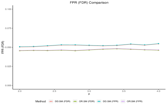
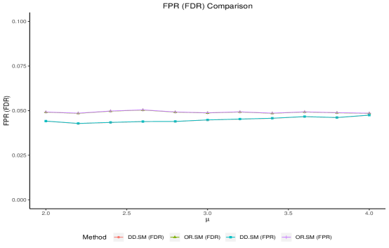
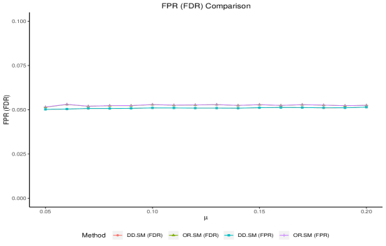
Figure 2: Dependent tests: Settings 1-3 are described in the main text. SMART controls the error rates at the nominal levels in most settings.

We apply the four methods to the simulated data. The FPR, MDR and ESS (expected sample size) are computed based on the average of $100$ replications, and are plotted as functions of varied parameter values. The results are summarized in Figure 2. In Setting 3, the two oracle methods (OR.ST and OR.SM) are not implemented as recursive formulae for $T_{OR}^{i,j}$ are unavailable.

We can see that all four methods control the FPR at the nominal level. However, the two single thresholding methods (OR.TH and DD.TH) are very conservative (the actual FPR is only about half of the nominal level). Similarly, both OR.TH and DD.TH are very conservative for MDR control. Specifically, $\tilde{\boldsymbol{\delta}}_{OR}$ operates as $p$ parallel SPRTs and suffers from the overshoot problem. The approximation errors of SPRTs can be greatly reduced by SMART that employs the compound thresholding strategy. We can see that the SMART procedures (OR.SM and DD.SM) control the error rates more accurately and require smaller sample sizes. When signals are sparse and weak (top middle panel), the MDR level of DD.SM is slightly higher than the nominal level. This is due to the estimation errors occurred at stage 1. It is of interest to develop more accurate estimation procedures in such settings. The FDR and FPR levels are similar for OR.SM and DD.SM. See Figure 2 in the supplement for details.

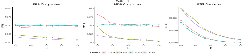
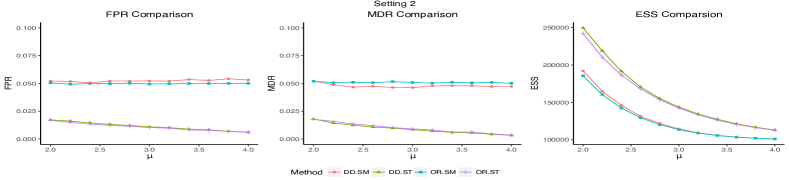
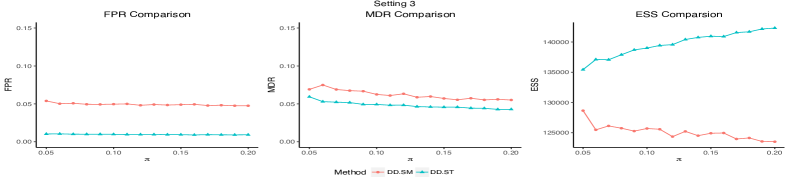
Figure 2: Comparison with single thresholding. The displayed procedures are DD.SM ($\bullet$), OR.SM ($\blacksquare$), DD.ST ($\blacktriangle$), OR.ST ($+$).

5.2 SMART vs. distilled sensing

This simulation study compares SMART and DS Haupt et al. (2011). As DS does not provide precise error rates control, the simulation is designed in the following way to make the comparison on an equal footing: we first run DS with up to 10 stages and record its FPR and MDR levels. Then we apply SMART at the corresponding FPR and MDR levels so that the two methods have roughly equal error rates. The ESS is used to compare the efficiency.

The data are generated from the multistage model (3.3). The number of locations is $p=10^{5}$. The following two settings are considered:

Setting 1: $\pi=0.05$. $\eta_{i}=\mu_{0}$ for all $i$. Vary $\mu_{0}$ from 2 to 4 with step size 0.2.

Setting 2: Draw $\eta_{i}$ randomly from $\mathcal{U}(2,4)$. Vary $\pi$ from $0.05$ to $0.2$.

In both settings, the FPR, MDR and ESS are computed by averaging over $100$ replications, and are plotted as functions of varied parameter values. The results are summarized in Figure 3.

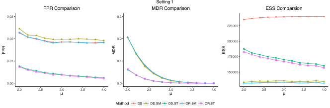
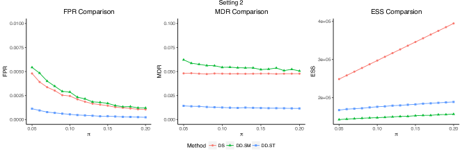
Figure 3: Comparison with DS. SMART outperforms DS in the sense that it achieves the same FPR and MDR levels with much smaller sample sizes.

We can see that the error rates of both OR.SM and DD.SM match well with those of DS, but they require fewer samples. OR.ST and DD.ST also outperform DS, achieving lower error rates with fewer samples. DD.SM controls the error rates more accurately compared to DD.ST, and requires fewer samples.

5.3 SMART vs. the Hunt procedure

This section conducts simulation studies to compare SMART with the multi-stage testing procedure proposed in Posch et al. (2009), which is denoted “Hunt” subsequently. We set the nominal FDR and MDR levels to be 0.05 and generate $m=10^{5}$ observations from a two group mixture model $(1-\pi)N(0,1)+\pi N(\mu_{i},1)$. We consider two settings:

• Setting 1: Vary $\pi$ from 0.05 to 0.2 and generate $\mu_{i}\sim\mathcal{U}(2,4)$.

• Setting 2: Fix $\pi=0.05$. Let $\mu_{i}=\mu$, vary $\mu$ from 2 to 4.

We apply Hunt and data-driven SMART and compute the FDR, MDR and the total sample size by averaging results in 100 replications. The Hunt method operates under a fixed stage regime; we fix the number of stages to be 2 for illustration. The sample size required for the Hunt procedure is always $2m=2\times 10^{5}$. The simulation results are summarized in Figure 4. We can see that SMART effectively controls both the FPR and MDR. By contrast, Hunt controls the FDR but does not control the MDR. This is because Hunt is not designed to control the false negative rates. Moreover, SMART requires a smaller sample size to achieve effective error rate control. The intuition is that the group sequential design adopted by Hunt does not eliminate the null coordinates in the first stage; this leads to loss in efficiency and higher study costs.

Figure 4: SMART vs Hunt. Top and bottom rows correspond to Settings 1 & 2.

5.4 Robustness of SMART under dependence

Our method and theory assume independence of observations across the coordinates. However, the independence assumption may be violated in practice. This section carries out additional numerical studies with correlated error terms across locations to investigate the robustness of the proposed SMART algorithm.

For the sequential testing setup, we first generate non-null effects from $\mathcal{U}(2,4)$ at $p=10^{4}$ locations. Then we apply the single thresholding procedure $\tilde{\boldsymbol{\delta}}_{OR}$ and SMART procedure $\boldsymbol{\delta}_{SM}$ to simulated data with correlation structures described in Settings 1-3 below. We use the computational algorithm described in Section 3.3. The FDR, MDR and ESS (expected sample sizes) are then calculated based on averaging results from $200$ data sets, and finally plotted as functions of the non-null proportion $\pi$. The simulation results are summarized in Fig. 2.

• Setting 1 (Gaussian process): the error terms are generated from a zero-mean Gaussian process with the covariance functions

  $$C(r)=e^{-r^{2}},\;\mbox{with }r\geq 0\text{ being the distance between two locations.}$$

• Setting 2 (Tridiagonal): the error terms are generated from a multivariate normal distribution with the following covariance matrix $\Sigma$:

  $$\Sigma_{i,i} = 1,\;i=1,\cdots,p,$$

  $$\Sigma_{i,i+1} = 0.5,\;i=1,\cdots,p-1,$$

  $$\Sigma_{i-1,i} = 0.5,\;i=2,\cdots,p,$$

  $$\Sigma_{i,i+2} = 0.4,\;i=1,\cdots,p-2,$$

  $$\Sigma_{i-2,i} = 0.4,\;i=3,\cdots,p.$$

  All other entries equal to zero.

• Setting 3 (Autoregressive model): the error terms are generated from a multivariate normal distribution with the following covariance matrix $\Sigma$:

  $$\Sigma_{i,j} = 0.5^{|i-j|},\;i,j=1,\cdots,p.$$

Figure 5: Dependent tests: Settings 1-3 are described in the main text. SMART controls the error rates at the nominal levels in most settings.

We observe some similar patterns as before. SMART (DD.SM) roughly controls the FPR at the nominal level when moderate correlations are present between locations. The single thresholding procedures with parallel SPRTs (DD.ST) are too conservative for error rates control in all settings. The resulting ESS of DD.ST is significantly larger than that is needed by DD.SM. In Setting 2 the FPR of SMART can be higher than the nominal level 0.05 but seems to be acceptable. SMART controls the MDR under the nominal level in all settings. Our simulation studies suggest that SMART has robust performance under a range of dependence structures. However, the scope of our empirical studies is limited and more numerical and theoretical support are needed for making definitive conclusions. Finally, we stress that it is still an open issue to develop multiple testing methods that incorporates informative correlation structures to improve efficiency Sun and Cai (2009); Sun et al. (2015). The modeling of spatial dependence in the sequential setting is complicated because we have a lot of missing data in later stages.

5.5 SMART for signal detection

SMART can be employed as a method for signal detection Donoho and Jin (2004). The goal is to test the global null hypothesis

$$H_{0}^{p}:\{X_{1},\cdots,X_{p}\}\;{\sim}\;F_{0}\mbox{ vs. }H_{1}^{p}:\{X_{1},\cdots,X_{p}\}\;{\sim}\;(1-\pi)F_{0}+\pi F_{1i}$$ (5.1)

for some $\pi>0$. This is a global inference problem that is very different from the simultaneous inference problem we have considered in previous sections. Comparing the detection boundaries derived in Donoho and Jin (2004) with the upper limit in Theorem 5, we can see that SMART requires fewer samples than non-adaptive testing schemes for separating $H_{0}^{p}$ and $H_{1}^{p}$ with negligible testing errors. Similar findings have been reported by Haupt et al. (2011).

This section carries out simulation studies to investigate the performance of SMART as a signal detection procedure. Specifically, SMART (Algorithm 1) eliminates noise locations stage by stage. If all coordinates are eliminated as noise locations eventually, then we do not reject the global null. If any coordinate is selected as signal, then we reject the global null. Under the global null $\pi=0$, the false discovery proportion (FDP) only takes two possible values: 0 (if no coordinate is selected as signal) and 1 (if at least one coordinate is selected as signal). It was argued by Benjamini and Hochberg (1995) that under the global null, the FPR cannot be controlled, whereas it is always possible to control the FDR. In our simulation, the FDR is calculated as the average of the FDPs over 200 replications; the average may be conceptualized as an estimate of the Type I error rate for testing the global null, i.e. the relative frequency for incorrectly rejecting the global null when $\pi=0$ among all repeated experiments.

Figure 6: SMART for signal detection: the FDR is used as the Type I error rate.

We apply SMART by setting $\alpha=\gamma=0.05$. The data are generated using the same models as those in previous sections except that we now let $\pi=0$. We vary the dimension $p$ from 100 to 5,000 and plot the corresponding FDRs. It can be seen that SMART controls the FDR at the nominal level 0.05 in all settings. The MDR and ESS are also reported. (If no true signals are discovered, then the MDR will be set as 0.) We conclude that SMART controls the Type I error rate for testing the global null.

6 Applications

In this section we apply the SMART procedure to A/B testing (Section 6.1), high-throughput screening (HTS, Section 6.2) and satellite image analysis (Section 6.3).

6.1 A/B Testing

A/B testing has become the golden standard for testing new ideas and building product launch plans in high-tech firms. This section illustrates the application of our SMART procedure to A/B testing using a real-world experiment at Snap Inc.. The quantity of interest is the average treatment effect (ATE) between the control and treatment arms (each arm consists of several hundred users). The ATEs are calculated on a daily basis for thousands of metrics. To save the study costs and speed up the decision process, we adopt an adaptive design to gradually narrow down (day by day) the set of metrics to be investigated. To check whether this application provides a suitable scenario for applying our SMART procedure, note that (a) it is reasonable to assume that the expected value of the ATE for a given metric is fixed over time, and (b) the ATEs, which are allowed to vary across testing units, are approximately normally distributed according to the central limit theorem. We conclude that the conditions (fixed $\mu_{i}$ over different stages and asymptotic normality of the summary statistic) required by our methodology have been fulfilled.

We analyze a data set from a multi-stage experiment with a running duration of 22 days. As the data are collected on a daily basis, it is natural to view that the experiment has 22 stages. At every stage, the ATEs are computed for a total of 1702 metrics and standardized as z-scores. We set the null distribution of the ATE statistic as $N(0,1)$. Under the alternative, the ATE statistic at unit $i$ has mean $\mu_{i}$. We assume that $\mu_{i}$ is fixed at all stages $j=1,2,\cdots$, and allow $\mu_{i}$ to vary across $i$. This justifies the use of the multi-stage model given by (3.3) and the computational algorithms described in Appendix C. The sparsity parameter $\hat{\pi}$ is estimated to be $\hat{\pi}\approx 0.15$ by applying Jin and Cai’s method (Jin and Cai, 2007) to the data collected on Day 1. The pre-specified FDR and MDR levels are $0.05$ and $0.2$, respectively.

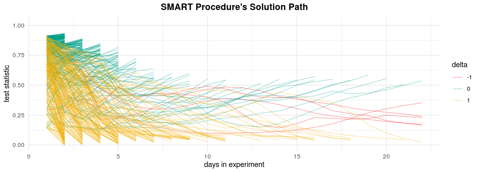
Figure 7: The solution path of our SMART procedure (data source: Snap Inc.): $\delta=1/0/-1$ respectively indicates rejected/accepted/undecided hypotheses.

The solution path of the SMART procedure is shown in Figure 7. We can see that by utilizing the adaptive design, definitive decisions on a large number of metrics can be made during earlier periods of the multi-stage experiment. This translates directly to great savings in data storage and pipeline calculations. Specifically, under the traditional A/B testing paradigm, one needs to collect data on 1,702 metrics throughout the 22-day duration. This requires a total of 44,252 measurements (each measurement corresponds to the cost of measuring one metric per day). By contrast, the SMART procedure only requires 3,541 measurements to localize important metrics with effective error rates control. We conclude that the new algorithm promises to save the study costs and greatly speed up the decision making process. Such benefits enable the company to quickly narrow down the list; hence the efforts and resources can be focused on improving a few core metrics that are pivotal for business.

6.2 Applications to HTS studies

The goal of the HTS study conducted by McKoy et al. (2012) is to identify novel inhibitors of the amyloid beta peptide ($A\beta$), whose aggregation is believed to be a trigger of the Alzheimer’s disease. In the study, a total of $p=51,840$ compounds are tested, with three measurements recorded for each compound. We use the observed data set as a pilot data set and simulate observations in later stages to illustrate how to design a multistage sampling and inference procedure for identifying useful compounds.

We compare the performances of different methods in two ways: (i) the total sample sizes needed to achieve pre-specified error rates, and (ii) the actual error rates achieved for a fixed total sample size. We first obtain z-scores based on the average of the three measurements and then estimate the non-null proportion and null distribution using the method in Jin and Cai (2007). The estimated non-null proportion is $\hat{\pi}\approx 0.0007$, and the estimated null distribution (referred to as the empirical null distribution, Efron (2004)) is $N(\hat{\mu}_{0},\hat{\sigma}_{0}^{2})$ with $\hat{\mu}_{0}=0.2459,\hat{\sigma}_{0}=0.6893$. Next, we choose the largest $100\hat{\pi}\%$ of the data and use their average as the signal amplitude $\hat{\mu}=3.194$. The observations in later stages will be generated based on the estimated parameters.

We set both the FDR and MDR at level $0.1$, apply SMART and record the total sample size. We then apply DS with the recorded sample size by SMART. The results are summarized below. Since DS always eliminates half of the locations at each step, for this particular instance DS requires at least $1.5p$ observations. We can see that with the sample size of $1.5p$, the DS method does not offer proper error rate control. The false positive proportion (FPP) is much higher than the nominal level.

Methods	FDP	MDP	Total Observation
SMART	0.083333	0.1081081	56926
DS	0.9971195	0	77641

Next, we run DS up to 10 stages. The recorded FPP and missed discovery proportion (MDP) levels are 0.23 and 0.027, respectively. Next we apply SMART by setting the nominal FPR and MDR levels as 0.23 and 0.027 and compare the required sample sizes. The results are summarized below. We can see that SMART control the FPP and MDP below those of DS. Meanwhile, the required sample size is significantly smaller compared to DS.

Methods	FPP	MDP	Total Observation
DS	0.2340426	0.02702703	104308
SMART	0.1487284	0.02162162	67850

6.3 Application to the Phoenix Deep Survey

In astronomical surveys, a common goal is to separate sparse targets of interest (stars, supernovas, or galaxies) from background noise. We consider a dataset from Phoenix Deep Survey (PDS), a multi-wavelength survey of a region over 2 degrees diameter in the southern constellation Phoenix. The data set is publicly available. Fig. 5(a) shows a telescope image from the PDS. It has $p=616\times 536=330,176$ pixels, among which $1131$ pixels exhibit signal amplitude of at least $2.98$. In practice we monitor the same region for a fixed period of time. After taking high resolution images, it is of interest to narrow down the focus quickly using a sequential testing procedure so that we can use limited computational resources to explore certain regions more closely. The image is converted into gray-scale with signal amplitudes standardized. Fig. 5(b) depicts a contaminated image with simulated Gaussian white noise.

For the first comparison, we apply SMART by setting both the FPR and MDR at $5\%$. The total number of measurements is recorded as 368,796. As a comparison, we apply DS with the recorded sample size, which is approximately $1.5p$. We can see that SMART control the error rates precisely. The resulting images for SMART and DS are demonstrated in Fig. 5(c) and (d), respectively. We can see SMART produces much sharper images than DS.

Methods	FPP	MDP	Total Observation
SMART	0.06321335	0.05658709	368796
DS	0.9864338	0.00265252	495866

For the second comparison, we first implement DS up to 12 stages. The corresponding FPP and MDP levels are recorded as 0.07 and 0.014. We then apply SMART by setting the nominal FPR and MDR at these recorded error rates. The corresponding true error rates and required sample sizes of the two methods are summarized below.

Methods	FDP	MDP	Total Observation
DS	0.07237937	0.01414677	670331
SMART	0.03192407	0.00795756	479214

We can see that SMART controls both the FPP and MDP below the nominal levels (0.07 and 0.014). The required sample size is also much smaller than DS. The resulting images for SMART and DS are shown in Fig. 5(e) and (f), we can see SMART produces slightly sharper images than its competitor DS.

(a) Original Data

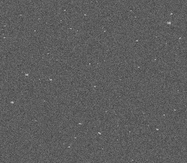
(b) Noisy Observation

(c) SMART result 1

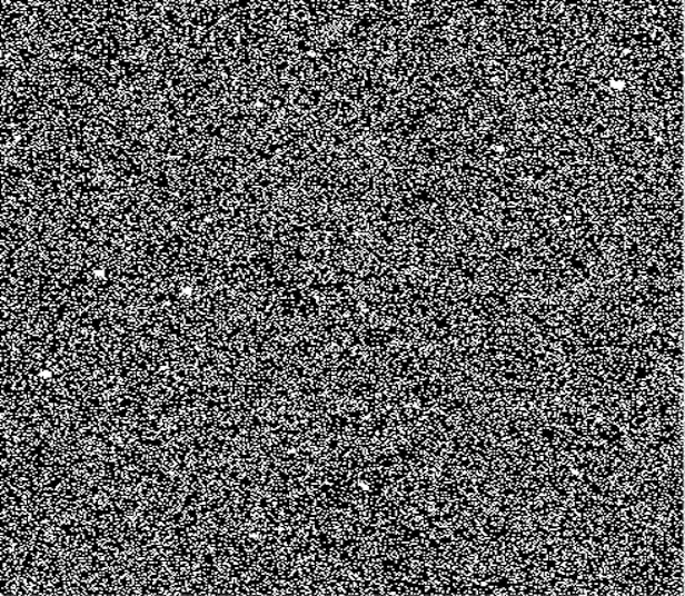
(d) DS result 1

(e) SMART result 2

(f) DS result 2

Figure 8: SMART and DS comparison. Fig. (a) and (b) show the original radio telescope image and tainted image with white noise, respectively. Fig. (c) and (d) compare SMART and DS when the total number of observations are about the same. Fig. (f) shows the resulting image when implementing DS for 12 stages, whereas Fig. (e) shows the image produced by SMART when using the recorded error rates from the 12-stage DS.

7 Discussion

The effectiveness of FPR/MDR control is a complicated issue that depends on several factors jointly. First, the reliable estimation of the stage-wise FPR/MDR requires a relatively large number of rejections, which in turn requires that the signals cannot be too sparse or too weak. Second, the consistent estimation of the non-null proportion requires that the detection and discovery boundaries (Cai and Sun, 2017) must be achieved. The impact of sparsity on the finite sample performance of SMART is investigated in Appendix D.1 of the Supplementary Material. Finally, the quality of density estimators depends on the sample size and smoothness of the underlying function. Our algorithm is designed to capitalize on copious data in ways not possible for procedures intended for moderate amounts of data, and SMART is most useful in large-scale testing scenarios where the structural information can be learned from data with good precision. An important future research direction is the development of precise estimation methods, which are instrumental for constructing powerful multi-stage testing procedures.

The proposed SMART procedure has several limitations. First, it assumes the effect size at a certain coordinate is fixed over time. This is a reasonable assumption for the three applications we considered in this article, where repeated measurements are taken on the same unknown effect sizes over time. However, in application scenarios such as multiple stage clinical trials, the end points or treatment effect sizes may vary from one stage to another. Second, the issue on multiple testing dependence needs much research. Our limited simulation results show that SMART remains to be valid under weak and positive dependences. It would be of great interest to justify such results theoretically. Moreover, the optimality issue under dependence remains unknown. We hope to pursue these directions in future research.

Supplementary Material for “Sparse Recovery With Multiple Data Streams: A Sequential Adaptive Testing Approach”

This file has four sections. We provide the proofs of all theorems (Appendix A), the derivations of the approximation formulae (2.8) (Appendix B) and the computation algorithm (Appendix C). Additional numerical results are provided in Appendix D.

A Proofs

A.1 Proof of Theorem 1

Proof.

Part (a) Denote $\boldsymbol{d}^{\pi}(t_{l},t_{u})=\{(N_{i},\delta_{i}):1\leq i\leq p\}$. Using the definition of $T_{OR}^{i,N_{i}}$, we have

$$\mathbb{E}\left\{\sum_{i=1}^{p}(1-\theta_{i})\delta_{i}\right\}=\mathbb{E}_{\boldsymbol{X}}\mathbb{E}_{\boldsymbol{\theta}|\boldsymbol{X}}\left\{\sum_{i=1}^{p}(1-\theta_{i})\delta_{i}\right\}=\mathbb{E}_{\boldsymbol{X}}\left(\sum_{i=1}^{p}T_{OR}^{i,N_{i}}\delta_{i}\right).$$

Then the FPR is $Q(t_{l},t_{u})={\mathbb{E}\left(\sum_{i=1}^{p}T_{OR}^{i,N_{i}}\delta_{i}\right)}/{\mathbb{E}\left(\sum_{i=1}^{p}\delta_{i}\right)}.$ It follows that

$$\mathbb{E}\left[\sum_{i=1}^{p}\left\{T_{OR}^{i,N_{i}}-Q(t_{l},t_{u})\right\}\mathbb{I}\left(T_{OR}^{i,N_{i}}\leq t_{l}\right)\right]=\mathbb{E}\left[\sum_{i:T_{OR}^{i,N_{i}}\leq t_{l}}\left\{T_{OR}^{i,N_{i}}-Q(t_{l},t_{u})\right\}\right]=0.$$

The above equation implies that $Q(t_{l},t_{u})\leq t_{l}$; otherwise every term on the LHS must be negative, resulting in a contradiction.

According to Assumption 1, $\mathbb{P}_{\theta_{i}}(N_{i}<\infty)=1$ for all $i$; see Berger (1985) for a proof. Since $\mathbb{P}_{\theta_{i}}(N_{i}<\infty)=1$ for all $i$, and $p$ is finite, we claim that $\mathbb{P}(\max{N_{i}}<\infty)=1$, i.e. the oracle procedure has a finite stopping time.

Next we prove that for a fixed $t_{u}$, $Q_{OR}(t_{l},t_{u})$ is non-decreasing in $t_{l}$. Let $Q_{OR}(t_{l,j},t_{u})=\alpha_{j}$ for $j=1,2$. We only need to show that if $t_{l,1}<t_{l,2}$, then $\alpha_{1}\leq\alpha_{2}$. Denote $N_{i,1}$ and $N_{i,2}$ the stopping times for location $i$ corresponding to thresholds $(t_{l,1},t_{u})$ and $(t_{l,2},t_{u})$, respectively. If $t_{l,1}<t_{l,2}$, then it is easy to see that for any particular realization of the experiment, we must have $N_{i,1}\geq N_{i,2}$.

We shall show that if $t_{l,1}<t_{l,2}$ and $\alpha_{1}>\alpha_{2}$, then we will have a contradiction. To see this, note that

$$\left(T_{OR}^{i,N_{i,2}}-\alpha_{2}\right)\mathbb{I}\left(T_{OR}^{i,N_{i,2}}\leq t_{l,2}\right)$$

$$= \left(T_{OR}^{i,N_{i,2}}-\alpha_{2}\right)\mathbb{I}\left(T_{OR}^{i,N_{i,2}}\leq t_{l,1}\right)+\left(T_{OR}^{i,N_{i,2}}-\alpha_{2}\right)\mathbb{I}\left(t_{l,1}<T_{OR}^{i,N_{i,2}}\leq t_{l,2}\right)$$

$$= \left(T_{OR}^{i,N_{i,1}}-\alpha_{2}\right)\mathbb{I}\left(T_{OR}^{i,N_{i,1}}\leq t_{l,1}\right)+\left(T_{OR}^{i,N_{i,2}}-\alpha_{2}\right)\mathbb{I}\left(t_{l,1}<T_{OR}^{i,N_{i,2}}\leq t_{l,2}\right)$$

$$\geq \left(T_{OR}^{i,N_{i,1}}-\alpha_{1}\right)\mathbb{I}\left(T_{OR}^{i,N_{i,1}}\leq t_{l,1}\right)+(\alpha_{1}-\alpha_{2})\mathbb{I}\left(T_{OR}^{i,N_{i,1}}\leq t_{l,1}\right)$$

$$+\left(T_{OR}^{i,N_{i,2}}-\alpha_{1}\right)\mathbb{I}\left(t_{l,1}<T_{OR}^{i,N_{i,2}}\leq t_{l,2}\right)$$

The second equality holds because if $T_{OR}^{i,N_{i,2}}<t_{l,1}$, then we must have $N_{i,1}=N_{i,2}$. Taking expectations on both sides, we have

$$\mathbb{E}\left\{\sum_{i=1}^{p}\left(T_{OR}^{i,N_{i,2}}-\alpha_{2}\right)\mathbb{I}\left(T_{OR}^{i,N_{i,2}}\leq t_{l,2}\right)\right\} = 0,\quad\mbox{and}$$

$$\mathbb{E}\left\{\sum_{i=1}^{p}\left(T_{OR}^{i,N_{i,1}}-\alpha_{1}\right)\mathbb{I}\left(T_{OR}^{i,N_{i,1}}\leq t_{l,1}\right)\right\} = 0.$$

However, since $\alpha_{1}>\alpha_{2}$ and $\alpha_{1}\leq t_{l,1}$ as shown previously, we must have

$$\mathbb{E}\left\{\sum_{i=1}^{p}(\alpha_{1}-\alpha_{2})\mathbb{I}\left(T_{OR}^{i,N_{i,1}}\leq t_{l,1}\right)\right\} >0,$$ and

$$\mathbb{E}\left\{\sum_{i=1}^{p}\left(T_{OR}^{i,N_{i,2}}-\alpha_{1}\right)\mathbb{I}\left(t_{l,1}<T_{OR}^{i,N_{i,2}}\leq t_{l,2}\right)\right\} \geq 0.$$

This leads to a contradiction. Therefore, we conclude that $Q_{OR}(t_{l},t_{u})$ is non-decreasing in $t_{l}$ for a fixed $t_{u}$.

Next, we prove that $\tilde{Q}(t_{l},t_{u})$ is non-increasing in $t_{u}$ for a fixed $t_{l}$. By the definition of MDR and similar arguments for the FPR part, we have

$$\mathbb{E}\left[\sum_{i=1}^{p}\left(1-T_{OR}^{i,N_{i}}\right)\left\{\mathbb{I}\left(T_{OR}^{i,N_{i}}\geq t_{u}\right)-\tilde{Q}(t_{l},t_{u})\right\}\right]=0.$$

Since our model has a finite stopping time, naturally we have

$$\left\{i:T_{OR}^{i,N_{i}}\geq t_{u}\right\}\cup\left\{j:T_{OR}^{j,N_{j}}\leq t_{l}\right\}=\left\{1,2,3,\cdots,p\right\}.$$

It follows that

$$\mathbb{E}\left[\textstyle\sum_{\left\{i:T_{OR}^{i,N_{i}}\geq t_{u}\right\}}\left(1-T_{OR}^{i,N_{i}}\right)\left\{1-\tilde{Q}(t_{l},t_{u})\right\}\right]=\mathbb{E}\left\{\textstyle\sum_{\left\{j:T_{OR}^{j,N_{j}}\leq t_{l}\right\}}\left(1-T_{OR}^{j,N_{j}}\right)\tilde{Q}(t_{l},t_{u})\right\}.$$

We have

$$\frac{1-\tilde{Q}(t_{l},t_{u})}{\tilde{Q}(t_{l},t_{u})}=\frac{\mathbb{E}\left\{\sum_{\left\{j:T_{OR}^{j,N_{j}}\leq t_{l}\right\}}\left(1-T_{OR}^{j,N_{j}}\right)\right\}}{\mathbb{E}\left\{\sum_{\left\{i:T_{OR}^{i,N_{i}}\geq t_{u}\right\}}\left(1-T_{OR}^{i,N_{i}}\right)\right\}}.$$ (A.1)

Consider two thresholds $t_{u,1}>t_{u,2}$. Denote $N_{i,1}$ and $N_{i,2}$ the corresponding stopping times at location $i$. The operation of the thresholding procedure implies that $N_{i,1}\geq N_{i,2}$, $\left\{i:T_{OR}^{i,N_{i,1}}\geq t_{u,1}\right\}\subset\left\{i:T_{OR}^{i,N_{i,2}}\geq t_{u,2}\right\}$, and $\left\{j:T_{OR}^{j,N_{j,2}}\leq t_{l}\right\}\subset\left\{j:T_{OR}^{j,N_{j,1}}\leq t_{l}\right\}$. Therefore,

$$\mathbb{E}\left\{\textstyle\sum_{\left\{i:T_{OR}^{i,N_{i,2}}\geq t_{u,2}\right\}}\left(1-T_{OR}^{i,N_{i,2}}\right)\right\}$$

$$= \mathbb{E}\left\{\textstyle\sum_{\left\{i:T_{OR}^{i,N_{i,2}}\geq t_{u,1}\right\}}\left(1-T_{OR}^{i,N_{i,2}}\right)\right\}+\mathbb{E}\left\{\textstyle\sum_{\left\{i:t_{u,1}>T_{OR}^{i,N_{2}}\geq t_{u,2}\right\}}\left(1-T_{OR}^{i,N_{i,2}}\right)\right\}$$

$$\geq \mathbb{E}\left\{\textstyle\sum_{\left\{i:T_{OR}^{i,N_{i,1}}\geq t_{u,1}\right\}}\left(1-T_{OR}^{i,N_{i,1}}\right)\right\}.$$

We have shown that $\left\{j:T_{OR}^{j,N_{j,2}}\leq t_{l}\right\}\subset\left\{j:T_{OR}^{j,N_{j,1}}\leq t_{l}\right\}$. Moreover, on the set $\left\{j:T_{OR}^{j,N_{j,2}}\leq t_{l}\right\}$, we have $N_{i,1}=N_{i,2}$. It follows that

$$\mathbb{E}\textstyle\left\{\sum_{\left\{j:T_{OR}^{j,N_{j,1}}\leq t_{l}\right\}}\left(1-T_{OR}^{j,N_{j,1}}\right)\right\}\geq\mathbb{E}\textstyle\left\{\sum_{\left\{j:T_{OR}^{j,N_{j,2}}\leq t_{l}\right\}}\left(1-T_{OR}^{j,N_{j,2}}\right)\right\}.$$

Combining the above results, we have

$$\frac{\mathbb{E}\textstyle\left\{\sum_{\left\{j:T_{OR}^{j,N_{j,1}}\leq t_{l}\right\}}\left(1-T_{OR}^{j,N_{j,1}}\right)\right\}}{\mathbb{E}\left\{\textstyle\sum_{\left\{i:T_{OR}^{i,N_{i,1}}\geq t_{u,1}\right\}}\left(1-T_{OR}^{i,N_{i,1}}\right)\right\}}\geq\frac{\mathbb{E}\textstyle\left\{\sum_{\left\{j:T_{OR}^{j,N_{j,2}}\leq t_{l}\right\}}\left(1-T_{OR}^{j,N_{j,2}}\right)\right\}}{\mathbb{E}\left\{\textstyle\sum_{\left\{i:T_{OR}^{i,N_{i,2}}\geq t_{u,2}\right\}}\left(1-T_{OR}^{i,N_{i,2}}\right)\right\}}.$$

Hence if $t_{u,1}>t_{u,2}$, then it follows from (A.1) that

$$\frac{1-\tilde{Q}(t_{l},t_{u,1})}{\tilde{Q}(t_{l},t_{u,1})}\geq\frac{1-\tilde{Q}(t_{l},t_{u,2})}{\tilde{Q}(t_{l},t_{u,2})}.$$

Therefore $\tilde{Q}(t_{l},t_{u,1})\leq\tilde{Q}(t_{l},t_{u,2})$. We conclude that $\tilde{Q}(t_{l},t_{u})$ is non-increasing in $t_{u}$ for a fixed $t_{l}$.

Part (b). The proof is divided into two parts. The first part describes a process that identifies a unique pair of oracle thresholds $(t_{OR}^{l},t_{OR}^{u})$. The second part shows that $\boldsymbol{d}^{\pi}(t_{OR}^{l},t_{OR}^{u})$ has the largest power among all eligible procedures.

(1). Oracle thresholds. Let $Q(1,1)=\bar{\alpha}$ be the theoretical upper bound corresponding to the FPR when all hypotheses are rejected. A prespecified FPR level $\alpha>0$ is called eligible if $\alpha<\bar{\alpha}$. Let $\mathcal{R}_{\alpha}=\{t_{u}:Q(t_{u},t_{u})>\alpha\}$. We can see that $\mathcal{R}_{\alpha}$ is nonempty if $\alpha$ is eligible, since $Q(0,0)=0$ and $Q(1,1)=\bar{\alpha}$. Consider $t_{u}\in\mathcal{R}_{\alpha}$. Note that $Q(0,t_{u})=0$ for all $t_{u}$, the following threshold is well defined:

$$t_{OR}^{l}(t_{u})=\sup\{t_{l}:Q(t_{l},t_{u})\leq\alpha\}.$$ (A.2)

We claim that $Q\{t_{OR}^{l}(t_{u}),t_{u}\}=\alpha$.

We prove by contradiction. First, according to the continuity of $Q(t_{l},t_{u})$, for every $t_{u}\in R_{\alpha}$, we can find $t_{l}^{*}(t_{u})$ such that $Q\left(t_{l}^{*}(t_{u}),t_{u}\right)=\alpha$ [since $Q(0,t_{u})=0$ and $Q(t_{u},t_{u})>\alpha$]. If not the equality does not hold, i.e. we have

$$Q\{t_{OR}^{l}(t_{u}),t_{u}\}<\alpha,$$

then the monotonicity of $Q(t_{l},t_{u})$ implies that $t_{l}^{*}(t_{u})>t_{OR}^{l}(t_{u})$, which contradicts the definition of $t_{OR}^{l}(t_{u})$. The above construction shows that, for every $t_{u}\in\mathcal{R}_{\alpha}$, we can always identify a unique $t_{OR}^{l}(t_{u})$ such that $Q\left\{t_{OR}^{l}(t_{u}),t_{u}\right\}=\alpha$.

We say $(\alpha,\gamma)$ constitute an eligible pair of prespecified error rates if $\alpha$ is eligible, and for this $\alpha$, $\gamma$ satisfies

$$0<\gamma<\sup\left\{\tilde{Q}\left(t^{l}_{OR}(t_{u}),t_{u}\right):t_{u}\in R_{\alpha}\right\}.$$

In the above definition, the eligibility of $(\alpha,\gamma)$ only depends on the model, but not any given $t_{u}$. Now consider an eligible pair $(\alpha,\gamma)$. The continuity of $\tilde{Q}_{u}(t_{u})\equiv\tilde{Q}\{t^{l}_{OR}(t_{u}),t_{u}\}$ implies that we can find $t_{u}^{*}$ such that $\tilde{Q}\left\{t^{l}_{OR}(t_{u}^{*}),t_{u}^{*}\right\}=\gamma$. Let

$$t_{OR}^{u}=\inf\{t_{u}\in R_{\alpha}:\tilde{Q}(t_{OR}^{l}(t_{u}),t_{u})=\gamma\}.$$

The pair of oracle thresholds are thus given by

$$(t^{l}_{OR},t^{u}_{OR})\equiv\{t^{l}_{OR}(t_{OR}^{u}),t^{u}_{OR}\}.$$

(2). Proof of optimality. Denote $\boldsymbol{d}_{*}=(\boldsymbol{N}_{*},\boldsymbol{\delta}_{*})$ a sequential procedure that satisfies $\mbox{FPR}(\boldsymbol{d}_{*})=\alpha_{*}\leq\alpha,\;\mbox{MDR}(\boldsymbol{d}_{*})=\gamma_{*}\leq\gamma,$ where $\boldsymbol{N}_{*}=(N_{*}^{1},\cdots,N_{*}^{p})$ and $\boldsymbol{\delta}_{*}=(\delta_{*}^{1},\cdots,\delta_{*}^{p})$ are the corresponding stopping times and decision rules. Deonte ESS$(\boldsymbol{d}_{*})$ the expected average stopping times. By definition, we have

$$\mathbb{E}\left\{\sum_{i=1}^{p}(T_{OR}^{i,N_{*}^{i}}-\alpha_{*})\delta_{*}^{i}\right\}=0,\quad\mathbb{E}\left\{\sum_{i=1}^{p}(1-T_{OR}^{i,N_{*}^{i}})(1-\delta_{*}^{i}-\gamma_{*})\right\}=0.$$

Now we can sort $T_{OR}^{i,N_{*}^{i}}$ as

$$T_{OR}^{(1),N_{*}^{(1)}}\leq T_{OR}^{(2),N_{*}^{(2)}}\leq\cdots\leq T_{OR}^{(p),N_{*}^{(p)}}$$

with their corresponding decisions $\delta_{*}^{(1)},\delta_{*}^{(2)},\cdots,\delta_{*}^{(p)}.$ If $\boldsymbol{\delta}_{*}$ does not take the following form of decision rule

$$\mbox{there exists a $k$},\mbox{ such that }\delta_{*}^{(i)}=\begin{cases}1&i\leq k\\ 0&k<i\leq p\end{cases},$$ (A.3)

then we can always modify $\boldsymbol{\delta_{*}}$ into such a form with the same ESS and smaller FPR and MDR. Specifically, suppose that there exists $l_{1}<l_{2}$ such that $\delta_{*}^{(l_{1})}=0$ and $\delta_{*}^{(l_{2})}=1$, then we swap these two decisions. Such operation can be iterated until the decision rule takes the form as (A.3). Denote the new decision rule by $\boldsymbol{d}_{*}^{\prime}=(\boldsymbol{N}_{*},\boldsymbol{\delta}_{*}^{\prime})$. Since $T_{OR}^{(l_{1}),N_{*}^{(l_{1})}}\leq T_{OR}^{(l_{2}),N_{*}^{(l_{2})}}$ in each swapping, we can reduce the FPR and MDR:

$$\alpha_{*}^{\prime} = \frac{\sum_{i=1}^{p}\left(T_{OR}^{i,N_{*}^{i}}\delta_{*}^{\prime i}\right)}{\mathbb{E}\left(\sum_{i=1}^{p}\delta_{*}^{\prime i}\right)}\leq\frac{\sum_{i=1}^{p}\left(T_{OR}^{i,N_{*}^{i}}\delta_{*}^{i}\right)}{\mathbb{E}\left(\sum_{i=1}^{p}\delta_{*}^{i}\right)}=\alpha_{*},$$

$$\gamma_{*}^{\prime} = \frac{\sum_{i=1}^{p}\left\{(1-T_{OR}^{i,N_{*}^{i}})(1-\delta_{*}^{\prime i})\right\}}{p\pi}$$

$$\leq\frac{\sum_{i=1}^{p}\left\{(1-T_{OR}^{i,N_{*}^{i}})(1-\delta_{*}^{i})\right\}}{p\pi}=\gamma_{*}.$$

Expressing $\boldsymbol{d}_{*}^{\prime}$ in the form of (2.2), we can find $t_{l}^{\prime}$ and $t_{u}^{\prime}$ such that

$${\delta}_{i,N_{i}}=\begin{cases}1&T_{OR}^{i,N_{i}}\leq t_{l}^{\prime}\\ 0&T_{OR}^{i,N_{i}}\geq t_{u}^{\prime}\end{cases},$$

where $Q(t_{l}^{\prime},t_{u}^{\prime})=\alpha_{*}^{\prime},\;\tilde{Q}(t_{l}^{\prime},t_{u}^{\prime})=\gamma_{*}^{\prime}$.

Now we claim that $t_{l}^{\prime}\leq t_{OR}^{l}(t_{OR}^{u})$ and $t_{u}^{\prime}\geq t_{OR}^{u}$. We prove by contradiction. First, if we have $t_{OR}^{u}>t_{u}^{\prime}$, then by the definition of $t_{OR}^{u}$, we have

$$\tilde{Q}\left(t_{OR}^{l}(t_{u}^{\prime}),t_{u}^{\prime}\right)>\gamma,\;Q\left(t_{OR}^{l}(t_{u}^{\prime}),t_{u}^{\prime}\right)=\alpha.$$

However, we also have $\tilde{Q}\left(t_{l}^{\prime},t_{u}^{\prime}\right)=\gamma_{*}^{\prime}\leq\gamma.$ By the definition of $\tilde{Q}(t_{l},t_{u})$, with the same $t_{u}$, only a larger $t_{l}$ could result in a strictly smaller MDR level. Together with the monotonicity of $\tilde{Q}(t_{l},t_{u})$ for a fixed $t_{u}$, we claim that $t_{OR}^{l}(t_{u}^{\prime})<t_{l}^{\prime}$. Since $Q(t_{l},t_{u})$ is non-decreasing in $t_{l}$ for a fixed $t_{u}$, we have $Q\left(t_{OR}^{l}(t_{u}^{\prime}),t_{u}^{\prime}\right)=\alpha$. It follows that $Q\left(t_{l}^{\prime},t_{u}^{\prime}\right)>\alpha,$ contradicting the fact that $Q(t_{l}^{\prime},t_{u}^{\prime})=\alpha_{*}^{\prime}\leq\alpha$. Therefore we must have $t_{u}^{\prime}\geq t_{OR}^{u}$.

Next, assume that $t_{l}^{\prime}>t_{OR}^{l}(t_{OR}^{u})$. Then by the definition of $t_{OR}^{l}(t_{u})$ and monotonicity of $Q(t_{l},t_{u})$, we have $Q\left(t_{l}^{\prime},t_{OR}^{u}\right)>\alpha$. Given the fact that $Q(t_{l}^{\prime},t_{OR}^{u})\leq t_{l}^{\prime}$, we must have $\alpha<t_{l}^{\prime}$, claiming that $t_{l}^{\prime}$ is always bounded below by $\alpha$ regardless of $\alpha_{*}^{\prime}$, which leads to a contradiction since we always have $Q(t_{l}^{\prime},t_{u}^{\prime})=\alpha_{*}^{\prime}<t_{l}^{\prime}$. Hence we must have $t_{l}^{\prime}\leq t_{OR}^{l}(t_{OR}^{u})$. Therefore

$$\text{ESS}(\boldsymbol{d}_{*}^{\prime})=\text{ESS}(\boldsymbol{d}_{*})\geq\text{ESS}(\boldsymbol{d}_{OR})$$

and the desired result follows.

∎

A.2 Proof of Theorem 2

Proof.

The goal is to show that the pair $t_{OR}^{l}=\alpha$ and $t_{OR}^{u}=\frac{1-\pi}{\pi\gamma+1-\pi}$ control the FPR and MDR. The FPR part is straightforward since according to the definition of $T_{OR}^{i,N_{i}}$, we have

$$\text{FPR}(\tilde{\boldsymbol{d}}_{OR})=\frac{\mathbb{E}\left\{\sum_{i=1}^{p}T_{OR}^{i,N_{i}}\mathbb{I}(T_{OR}^{i,N_{i}}\leq\alpha)\right\}}{\mathbb{E}\left\{\sum_{i=1}^{p}\mathbb{I}(T_{OR}^{i,N_{i}}\leq\alpha)\right\}}\leq\frac{\mathbb{E}\left\{\sum_{i=1}^{p}\alpha\cdot\mathbb{I}(T_{OR}^{i,N_{i}}\leq\alpha)\right\}}{\mathbb{E}\left\{\sum_{i=1}^{p}\mathbb{I}(T_{OR}^{i,N_{i}}\leq\alpha)\right\}}=\alpha.$$

Similarly for the FDR control, we have

$$\text{FDR}(\tilde{\boldsymbol{d}}_{OR})=\mathbb{E}\left\{\frac{\sum_{i=1}^{p}T_{OR}^{i,N_{i}}\mathbb{I}(T_{OR}^{i,N_{i}}\leq\alpha)}{\sum_{i=1}^{p}\mathbb{I}(T_{OR}^{i,N_{i}}\leq\alpha)\vee 1}\right\}\leq\frac{\mathbb{E}\left\{\sum_{i=1}^{p}\alpha\cdot\mathbb{I}(T_{OR}^{i,N_{i}}\leq\alpha)\right\}}{\mathbb{E}\left\{\sum_{i=1}^{p}\mathbb{I}(T_{OR}^{i,N_{i}}\leq\alpha)\vee 1\right\}}\leq\alpha.$$

Remark 4.

From the proof we can see that the choice of $t_{OR}^{l}=\alpha$, derived based on Wald’s approximation, can be conservative in practice.

To show the MDR part, we first carry out an analysis of the false negative rate (FNR), which is defined as

$$\text{FNR}(\tilde{\boldsymbol{d}}_{OR})=\frac{\mathbb{E}\left\{\sum_{i=1}^{p}\theta_{i}(1-\delta_{i})\right\}}{\mathbb{E}\left\{\sum_{i=1}^{p}(1-\delta_{i})\right\}}.$$

According to the operation of $\tilde{\boldsymbol{d}}_{OR}$, the FNR can be further calculated as

$$\text{FNR}(\tilde{\boldsymbol{d}}_{OR}) = \frac{\mathbb{E}\left\{\sum_{i=1}^{p}(1-T_{OR}^{i,N_{i}})\mathbb{I}(T_{OR}^{i,N_{i}}\geq t_{u})\right\}}{\mathbb{E}\left\{\sum_{i=1}^{p}\mathbb{I}(T_{OR}^{i,N_{i}}\geq t_{u})\right\}}$$

$$\leq 1-t_{u}=\frac{\pi\gamma}{\pi\gamma+1-\pi}.$$

Denote $\tilde{\boldsymbol{d}}_{OR}^{i}=(\tilde{N}_{OR}^{i},\tilde{\delta}_{OR}^{i})$. We have shown that $\text{FPR}(\tilde{\boldsymbol{d}}_{OR})\leq\alpha$. Suppose the actual FPR level is $\tilde{\alpha}\leq\alpha$. Then $\mathbb{E}\left\{\sum_{i=1}^{p}(1-\theta_{i})\tilde{\delta}_{OR}^{i}\right\}=\tilde{\alpha}(\sum_{i=1}^{p}\tilde{\delta}_{OR}^{i})$. It follows that

$$(1-\tilde{\alpha})\mathbb{E}\left(\textstyle\sum_{i=1}^{p}\tilde{\delta}_{OR}^{i}\right)=\mathbb{E}\textstyle\left\{\sum_{i=1}^{p}\theta_{i}\tilde{\delta}_{OR}^{i}\right\}.$$ (A.4)

Meanwhile, our analysis of the FNR shows that

$$\mathbb{E}\left\{\sum_{i=1}^{p}\theta_{i}(1-\tilde{\delta}_{OR}^{i})\right\}\leq\frac{\pi\gamma}{\pi\gamma+1-\pi}\cdot\mathbb{E}\left\{\sum_{i=1}^{p}(1-\tilde{\delta}_{OR}^{i})\right\}.$$ (A.5)

Combining (A.4) and (A.5), we obtain

$$\left(\pi\gamma+1-\pi\right)\left\{p\pi-(1-\tilde{\alpha})\mathbb{E}\left(\textstyle\sum_{i=1}^{p}\tilde{\delta}_{OR}^{i}\right)\right\}\leq\pi\gamma\left\{p-\mathbb{E}\left(\textstyle\sum_{i=1}^{p}\tilde{\delta}_{OR}^{i}\right)\right\}.$$

It follows that

$$\mathbb{E}\left(\sum_{i=1}^{p}\tilde{\delta}_{OR}^{i}\right)\geq\frac{p\pi(1-\pi)(1-\gamma)}{-\pi\gamma\tilde{\alpha}+(1-\pi)(1-\tilde{\alpha})}\geq\frac{p\pi(1-\gamma)}{(1-\tilde{\alpha})}$$

Using (A.4) and $p\pi=\mathbb{E}(\sum_{i}\theta_{i})$, we have

$$\mathbb{E}(\textstyle\sum_{i=1}^{p}\theta_{i}\tilde{\delta}_{OR}^{i})\geq\mathbb{E}(\sum_{i=1}^{p}\theta_{i})-\gamma\mathbb{E}(\sum_{i=1}^{p}\theta_{i}).$$

Therefore $\mathbb{E}\{\sum_{i=1}^{p}\theta_{i}(1-\tilde{\delta}_{OR}^{i})\}\leq\gamma\mathbb{E}(\sum_{i=1}^{p}\theta_{i})$ and the desired result follows. ∎

A.3 Proof of Theorem 3

Proof.

Part (i). The FPR and FDR control. To show the validity of SMART for FPR control, we utilize the idea in Efron (2008); Cai and Sun (2009) for group-wise testing. Define stage-wise false positive rate $\text{sFPR}_{j}$ as

$$\text{sFPR}_{j}:=\frac{\mathbb{E}\left\{\sum_{i\in\mathcal{S}_{j}}(1-\theta_{i})\delta_{i}\right\}}{\mathbb{E}\sum_{i\in\mathcal{S}_{j}}\delta_{i}},$$

where $\text{sFPR}_{j}$ is the ratio of the expected number of false rejections at stage $j$ over the expected number of all rejections at stage $j$. The first step is to show that SMART controls all stage-wise FDRs at level $\alpha$. The second step is to show that the global FDR is controlled at level $\alpha$ by combining hypotheses rejected from all stages. By our definition of $\text{sFPR}_{j}$, we have

$$\text{sFPR}_{j}=\frac{\mathbb{E}\left(\sum_{i=1}^{k_{j}^{s}}T_{OR}^{(i),j}\right)}{\mathbb{E}\left(k_{j}^{s}\right)}\leq\frac{\mathbb{E}\left(k_{j}^{s}\alpha\right)}{\mathbb{E}\left(k_{j}^{s}\right)}=\alpha.$$

Therefore SMART controls the sFPR at level $\alpha$ across all stages.

Next we show that if $\text{sFPR}_{j}$ is controlled universally at pre-specified levels across all stages, then the global FPR will be controlled at the same level. Let $N_{SM}$ denote the total number of stages that $\boldsymbol{d}_{SM}$ has. It follows that

$$\text{FPR}(\boldsymbol{d}_{SM}) = \frac{\mathbb{E}\left\{\sum_{j=1}^{N_{SM}}\sum_{i\in\mathcal{S}_{j}}\left(1-\theta_{i}\right)\delta^{i}_{SM}\right\}}{\mathbb{E}\left(\sum_{j=1}^{N_{SM}}\sum_{i\in\mathcal{S}_{j}}\delta^{i}_{SM}\right)}$$

$$\leq \frac{\mathbb{E}\left(\sum_{j=1}^{N_{SM}}\alpha\sum_{i\in\mathcal{S}_{j}}\delta^{i}_{SM}\right)}{\mathbb{E}\left(\sum_{j=1}^{N_{SM}}\sum_{i\in\mathcal{S}_{j}}\delta^{i}_{SM}\right)}=\alpha.$$

Consider the quantity $\mathbb{E}\left\{\sum_{j=1}^{N_{SM}}\sum_{i\in\mathcal{S}_{j}}\left(1-\theta_{i}\right)\delta^{i}_{SM}\right\}$. Note that $i\in\mathcal{S}_{j}$ indicates that (i) a total of $j$ data points $\boldsymbol{x}_{i}^{j}=(x_{i}^{1},\cdots,x_{i}^{j})$ are eventually collected for the $i$th unit and (ii) a decision for unit $i$ is made at stage $j$. It follows that $\boldsymbol{\delta}_{SM}^{i}$ only depends on $\boldsymbol{x}_{i}^{j}$ and can be factored out:

$$\mathbb{E}\left\{\sum_{j=1}^{N_{SM}}\sum_{i\in\mathcal{S}_{j}}\left(1-\theta_{i}\right)\delta^{i}_{SM}\right\} = \mathbb{E}\left\{\sum_{j=1}^{N_{SM}}\sum_{i\in\mathcal{S}_{j}}\mathbb{E}\left[\left(1-\theta_{i}\right)\delta^{i}_{SM}|\boldsymbol{x}_{i}^{j}\right]\right\}$$

$$= \mathbb{E}\left\{\sum_{j=1}^{N_{SM}}\sum_{i\in\mathcal{S}_{j}}\delta^{i}_{SM}\mathbb{E}\left[\left(1-\theta_{i}\right)|\boldsymbol{x}_{i}^{j}\right]\right\}$$

According to the definition of the oracle statistic, We have

$$\mathbb{E}\left\{\sum_{j=1}^{N_{SM}}\sum_{i\in\mathcal{S}_{j}}\left(1-\theta_{i}\right)\delta^{i}_{SM}\right\}=\mathbb{E}\left\{\sum_{j=1}^{N_{SM}}\sum_{i\in\mathcal{S}_{j}}\delta^{i}_{SM}T_{OR}^{i,j}\right\}\leq\mathbb{E}\left\{\sum_{j=1}^{N_{SM}}\alpha\sum_{i\in\mathcal{S}_{j}}\delta^{i}_{SM}\right\}.$$

The last inequality is due to the operation of SMART, which ensures that at every stage $j$, we always have $\sum_{i\in\mathcal{S}_{j}}T_{OR}^{i,j}\delta^{i}_{SM}\leq\alpha\sum_{i\in\mathcal{S}_{j}}\delta^{i}_{SM}.$ Therefore we have

$$\text{FPR}(\boldsymbol{d}_{SM})\leq\frac{\mathbb{E}\left(\sum_{j=1}^{N_{SM}}\alpha\sum_{i\in\mathcal{S}_{j}}\delta^{i}_{SM}\right)}{\mathbb{E}\left(\sum_{j=1}^{N_{SM}}\sum_{i\in\mathcal{S}_{j}}\delta^{i}_{SM}\right)}=\alpha.$$

Similarly, we can prove the global FDR control by jointly evaluating the performance SMART at separate stages

$$\text{FDR}(\boldsymbol{d}_{SM}) = \mathbb{E}\left\{\frac{\sum_{j=1}^{N_{SM}}\sum_{i\in\mathcal{S}_{j}}\left(1-\theta_{i}\right)\delta^{i}_{SM}}{(\sum_{j=1}^{N_{SM}}\sum_{i\in\mathcal{S}_{j}}\delta^{i}_{SM})\vee 1}\right\}$$

$$= \mathbb{E}\left[\frac{\sum_{j=1}^{N_{SM}}\sum_{i\in\mathcal{S}_{j}}T_{OR}^{i,j}\delta^{i}_{SM}}{\left(\sum_{j=1}^{N_{SM}}\sum_{i\in\mathcal{S}_{j}}\delta^{i}_{SM}\right)\vee 1}\right]\leq\alpha$$

The last inequality is due to the operation of SMART.

Part (ii). MDR control. Unlike the FDR analysis, stage-wise MDR control does not imply global MDR control. We introduce an intermediate quantity, the false non-discovery rate (FNR) and divide the proof into two steps: the first step shows that stage-wise FNR control implies global FNR control; the second step establishes the relationship between the global MDR and global FNR.

Define stage-wise false non-discovery rate $\text{sFNR}_{j}$ as

$$\text{sFNR}_{j}:=\frac{\mathbb{E}\left\{\sum_{i\in\mathcal{S}_{j}}\theta_{i}(1-\delta_{i})\right\}}{\mathbb{E}\sum_{i\in\mathcal{S}_{j}}(1-\delta_{i})},$$

where $\text{sFNR}_{j}$ is the ratio of the expected number of false non-discoveries over the expected number of all non-discoveries. It follows that

$$\text{sFNR}_{j}=\frac{\mathbb{E}\left\{\sum_{i=0}^{k_{j}^{e}-1}\left(1-T_{OR}^{k_{j}-i,j}\right)\right\}}{\mathbb{E}\left(k_{j}^{e}\right)}\leq\frac{\mathbb{E}\left(k_{j}^{e}\frac{\pi\gamma}{\pi\gamma+1-\pi}\right)}{\mathbb{E}\left(k_{j}^{e}\right)}=\frac{\pi\gamma}{\pi\gamma+1-\pi}.$$

Therefore SMART controls the sFNR at level $\frac{\pi\gamma}{\pi\gamma+1-\pi}$ across all stages. Next, we show that if $\text{sFNR}_{j}$ is controlled universally at pre-specified levels across all stages, then the global FNR will be controlled at the same level.

FNR $$= \frac{\mathbb{E}\left\{\sum_{j=1}^{N}\sum_{i\in\mathcal{S}_{j}}\theta_{i}\left(1-\delta^{i}_{SM}\right)\right\}}{\mathbb{E}\left\{\sum_{j=1}^{N}\sum_{i\in\mathcal{S}_{j}}\left(1-\delta^{i}_{SM}\right)\right\}}$$

$$\leq \frac{\mathbb{E}\left\{\sum_{j=1}^{N}\frac{\pi\gamma}{\pi\gamma+1-\pi}\sum_{i\in\mathcal{S}_{j}}\left(1-\delta^{i}_{SM}\right)\right\}}{\mathbb{E}\left\{\sum_{j=1}^{N}\sum_{i\in\mathcal{S}_{j}}\left(1-\delta^{i}_{SM}\right)\right\}}$$

$$= \frac{\pi\gamma}{\pi\gamma+1-\pi}.$$

Finally, according to the proof of Theorem 2 (Appendix), the MDR and FNR satisfy the following relationship

$$\mbox{$\mbox{MDR}\leq\gamma$ if $\text{FNR}\leq\frac{\pi\gamma}{\pi\gamma+1-\pi}$}.$$

We conclude that the MDR is controlled at level $\gamma$, completing the proof.

∎

A.4 Proof of Theorem 4

Proof.

For a symmetric decision procedure $\boldsymbol{d}$, denote its Type I and Type II errors on unit $i$ by $\alpha^{\prime}=\mathbb{P}_{H_{i,0}}(\mbox{Reject $H_{i,0}$})$ and $\gamma^{\prime}=\mathbb{P}_{H_{i,1}}(\mbox{Accept $H_{i,0}$}).$ It can be shown that the corresponding global error rates are given by

$$\text{FPR}(\boldsymbol{d})=\frac{(1-\pi)\alpha^{\prime}}{(1-\pi)\alpha^{\prime}+\pi(1-\gamma^{\prime})}\quad\mbox{and}\quad\text{MDR}(\boldsymbol{d})=\gamma^{\prime},$$ (A.6)

respectively. Our result largely follows from the lower bound derived in Malloy and Nowak (2014a) on family-wise error rate (FWER); we only highlight the main steps on how to go from the FWER paradigm to the FPR/MDR paradigm, which essentially involves exploiting the relationship (A.6). From Thm. 2.39 in Siegmund (1985), we have

$$\tau_{1} \geq\frac{\alpha^{\prime}\log(\frac{\alpha^{\prime}}{1-\gamma^{\prime}})+(1-\alpha^{\prime})\log(\frac{1-\alpha^{\prime}}{\gamma^{\prime}})}{D(\mathbb{F}_{0}||\mathbb{F}_{1})}\quad\mbox{and}$$

$$\tau_{2} \geq\frac{(1-\gamma^{\prime})\log{(\frac{(1-\gamma^{\prime}}{\alpha^{\prime}})}+\gamma^{\prime}\log{(\frac{\gamma^{\prime}}{1-\alpha^{\prime}})}}{D(\mathbb{F}_{1}||\mathbb{F}_{0})},$$

where $\tau_{1}$ and $\tau_{2}$ are the expected stopping times for null and non-null locations, respectively. Furthermore, from Malloy and Nowak (2014a), we have

$$\tau_{1}\geq\frac{(1-\alpha^{\prime})\log(\gamma^{\prime})^{-1}-\log{2}}{D(\mathbb{F}_{0}||\mathbb{F}_{1})},\;\tau_{2}\geq\frac{(1-\gamma^{\prime})\log(\alpha^{\prime})^{-1}-\log{2}}{D(\mathbb{F}_{1}||\mathbb{F}_{0})}.$$

Using the KL divergence $D_{KL}(F_{0},F_{1})=\max\left\{D(\mathbb{F}_{0}|\mathbb{F}_{1}),D(\mathbb{F}_{1}|\mathbb{F}_{0})\right\}$, the average stopping time of all locations satisfies

$$\tau = \frac{(p-p\pi)\tau_{1}+p\pi\tau_{2}}{p}$$ (A.7)

$$\geq \frac{(1-\pi)(1-\alpha^{\prime})\log(\gamma^{\prime})^{-1}+\pi(1-\gamma^{\prime})\log(\alpha^{\prime})^{-1}-\log{2}}{D_{KL}(F_{0},F_{1})}.$$

We consider two situations. If $\alpha^{\prime}\leq\gamma^{\prime}$, then

$$\tau\geq(1-\pi)(1-\gamma^{\prime})\log(\gamma^{\prime})^{-1}+\pi(1-\gamma^{\prime})\log(\gamma^{\prime})^{-1}-\log{2}.$$

Note that for $0\leq x\leq 1$, $\{x\log x:x\in(0,1)\}$ reaches its minimum when $x=e^{-1}$. It follows that $2^{-1}<e^{-1/e}\leq{\gamma^{\prime}}^{\gamma^{\prime}}\leq 1$. Therefore

$$(1-\gamma^{\prime})\log(\gamma^{\prime})^{-1}\geq\log(2\gamma^{\prime})^{-1}.$$

Together with (A.7), we have $\tau\geq\frac{\log{(4\gamma^{\prime})^{-1}}}{D_{KL}(F_{0},F_{1})}.$ According to our constraint on $\tau$, we conclude that

$${\log({4\eta})^{-1}}\geq\tau{D_{KL}(F_{0},F_{1})}\geq{\log(4\gamma^{\prime})^{-1}}.$$

Therefore, $\gamma^{\prime}\geq\eta$ and $R^{*}(\boldsymbol{d})\geq\eta$.

If $\gamma^{\prime}\leq\alpha^{\prime}$, then we can similarly show that

$$\tau\geq\frac{(1-\alpha^{\prime})\log{\alpha^{\prime}}^{-1}-\log{2}}{D_{KL}(F_{0},F_{1})}\geq\frac{\log{\frac{1}{2\alpha^{\prime}}}-\log{2}}{D_{KL}(F_{0},F_{1})}\geq\frac{\log{\frac{1}{4\alpha^{\prime}}}}{D_{KL}(F_{0},F_{1})}.$$

It follows that

$$\log({4\eta})^{-1}\geq\tau{D_{KL}(F_{0},F_{1})}\geq\log({4\alpha^{\prime}})^{-1},$$

which implies $\alpha^{\prime}\geq\eta$. Under the assumption that $\pi<\frac{1}{3}$ and $\eta\leq\frac{1}{2}$, we have $\eta\leq\frac{1}{2}\leq\frac{1-2\pi}{1-\pi}$. Consider the function $k(x)=\frac{\left(1-\pi\right)x}{\left(1-\pi\right)x+\pi}$. It is easy to see that $k(x)$ is monotonically increasing in $x$. Hence

$$R^{*}(\boldsymbol{d}) \geq\frac{(1-\pi)\alpha^{\prime}}{(1-\pi)\alpha^{\prime}+\pi(1-\gamma^{\prime})}\geq\frac{(1-\pi)\alpha^{\prime}}{(1-\pi)\alpha^{\prime}+\pi}$$

$$\geq\frac{(1-\pi)\eta}{(1-\pi)\eta+\pi}\geq\frac{(1-\pi)\eta}{(1-\pi)\frac{1-2\pi}{1-\pi}+\pi}=\eta,$$

completing the proof. ∎

A.5 Proof of Theorem 5

Proof.

We have already shown that when $t_{l}=\alpha$ and $t_{u}=\frac{1-\pi}{\pi\gamma+1-\pi}$, the SMART procedure controls the FDR and MDR at level $\alpha$ and $\gamma$, respectively. Let $\alpha=\gamma=\frac{1}{f(p)^{1+\epsilon}}$. With the choice of $t_{l}$ and $t_{u}$ mentioned above, we have

$$\lim_{p\rightarrow\infty}R^{*}(\boldsymbol{d})=\lim_{p\rightarrow\infty}\frac{2}{f(p)^{1+\epsilon}}=0,$$

which proves the first part of the theorem.

Next we establish the upper bound. Consider $p$ simultaneous SPRTs with the same threshold $t_{l}$ and $t_{u}$. The operation of our SMART procedure uses these thresholds for the moving averages; hence the SPRT approach with the same $t_{l}$ and $t_{u}$ will always take more samples. It is sufficient to show that the result holds for simultaneous SPRTs.

We first use the relationship (B.11) to convert thresholds $t_{l}$ and $t_{u}$ to the thresholds for SPRTs:

$$A=\frac{(1-\pi)(1-t_{u})}{\pi t_{u},},\quad B=\frac{(1-\pi)(1-t_{l})}{\pi t_{l}}.$$

Under our specifications, we further have

$$A=\frac{\gamma(1-\pi)}{\pi\gamma+1-\pi},\quad B=\frac{(1-\pi)(1-\alpha)}{\pi\alpha}.$$

From Siegmund (1985) (Equations 9-10, P10), we have

$$\alpha^{\prime} \leq B^{-1}(1-\gamma^{\prime})\leq B^{-1},$$

$$\gamma^{\prime} \leq A(1-\alpha^{\prime})\leq A.$$

According to Assumption (4.1), we have

$$\mathbb{E}(\log\mathcal{L}^{i,N_{i}}|\log\mathcal{L}^{i,N_{i}}<\log A) \geq \log A-C_{1},$$

$$\mathbb{E}(\log\mathcal{L}^{i,N_{i}}|\log\mathcal{L}^{i,N_{i}}>\log B) \leq \log B+C_{2}$$

for some positives constants $C_{1}$ and $C_{2}$. Consider $\mathbb{E}_{\theta_{i}=0}\left(\log\mathcal{L}^{i,N_{i}}\right)$. Then

$$-\mathbb{E}_{\theta_{i}=0}\left(\log\mathcal{L}^{i,N_{i}}\right)$$

$$= -(1-\alpha)\mathbb{E}_{\theta_{i}=0}\left(\log\mathcal{L}^{i,N_{i}}|\log\mathcal{L}^{i,N_{i}}<\log A\right)-\alpha\mathbb{E}_{\theta_{i}=0}(\log\mathcal{L}^{i,N_{i}}|\log\mathcal{L}^{i,N_{i}}>\log B)$$

$$\leq (1-\alpha)(\log A^{-1}+C_{1})-\alpha\log B$$

$$\leq (1-\alpha)(\log A^{-1}+C_{1})\leq\log A^{-1}+C_{1}.$$

Likewise, we can show that

$$\mathbb{E}_{\theta_{i}=1}(\log\mathcal{L}^{i,N_{i}})\leq\log B+C_{2}.$$

Let $C_{3}=(1-\pi)C_{1}+\pi C_{2}$. According to Wald’s identity (P490, Berger (1985)), we have

$$\mathbb{E}_{\theta_{i}=1}(N_{i}) = \frac{\mathbb{E}_{\theta_{i}=1}\left(\log\mathcal{L}^{i,N_{i}}\right)}{\mathbb{E}_{\theta_{i}=1}\left(\log\mathcal{L}^{i,1}\right)}=\frac{\mathbb{E}_{\theta_{i}=1}\left(\log\mathcal{L}^{i,N_{i}}\right)}{D(\mathbb{F}_{1}|\mathbb{F}_{0})},$$

$$\mathbb{E}_{\theta_{i}=0}(N_{i}) = \frac{\mathbb{E}_{\theta_{i}=0}\left(\log\mathcal{L}^{i,N_{i}}\right)}{\mathbb{E}_{\theta_{i}=0}\left(\log\mathcal{L}^{i,1}\right)}=\frac{-\mathbb{E}_{\theta_{i}=0}\left(\log\mathcal{L}^{i,N_{i}}\right)}{D(\mathbb{F}_{0}|\mathbb{F}_{1})}.$$

It follows that

$$\lim_{p\rightarrow\infty}\frac{\tau}{\log f(p)} = \lim_{p\rightarrow\infty}\frac{(1-\pi)\mathbb{E}_{\theta_{i}=0}(N_{i})+\pi\mathbb{E}_{\theta_{i}=1}(N_{i})}{\log f(p)}$$ (A.8)

$$\leq \lim_{p\rightarrow\infty}\frac{(1-\pi)(\log{A}^{-1}+C_{1})}{\log f(p)D(\mathbb{F}_{0}|\mathbb{F}_{1})}+\lim_{p\rightarrow\infty}\frac{\pi(\log{B}+C_{2})}{\log f(p)D(\mathbb{F}_{1}|\mathbb{F}_{0})}$$

$$= \lim_{p\rightarrow\infty}\frac{(1-\pi)\log{\frac{\pi\gamma+1-\pi}{\gamma(1-\pi)}}+\pi\log{\frac{(1-\pi)(1-\alpha)}{\pi\alpha}}+C_{3}}{\log f(p)\min\left\{(D(\mathbb{F}_{0}|\mathbb{F}_{1}),D(\mathbb{F}_{1}|\mathbb{F}_{0})\right\}}$$

$$= \lim_{p\rightarrow\infty}\frac{(1-\pi)\log({\gamma}^{-1})+\pi\log{\frac{(1-\pi)}{\pi\alpha}}+C_{3}}{\log f(p)\min\left\{(D(\mathbb{F}_{0}|\mathbb{F}_{1}),D(\mathbb{F}_{1}|\mathbb{F}_{0})\right\}}$$ (A.9)

$$= \lim_{p\rightarrow\infty}\frac{\log(\alpha^{-1})}{\log f(p)\min\left\{(D(\mathbb{F}_{0}|\mathbb{F}_{1}),D(\mathbb{F}_{1}|\mathbb{F}_{0})\right\}}$$

$$= \frac{1+\epsilon}{\min\left\{(D(\mathbb{F}_{0}|\mathbb{F}_{1}),D(\mathbb{F}_{1}|\mathbb{F}_{0})\right\}}.$$

From (A.8) to (A.9), we have used the fact $\alpha$ and $\gamma$ are error rates converging to zero; hence

$$\frac{\pi\gamma+1-\pi}{\gamma(1-\pi)} = \frac{1}{\gamma}\{1+o(1)\}$$

$$\frac{(1-\pi)(1-\alpha)}{\pi\alpha} = \frac{(1-\pi)}{\pi\alpha}\{1+o(1)\}.$$

Equation (A.5) uses the fact that $\alpha=\gamma$. The desired result follows. ∎

B Derivation of thresholds

We need the following assumption in our derivation. The assumption has been commonly adopted in the literature on SPRT (e.g. Berger (1985); Siegmund (1985)).

Assumption 2.

Consider $Z_{i,1}$ defined in Assumption 1. For all $i$, we have $\mathbb{P}_{\theta_{i}}(Z_{i,1}=0)<1$, $\mathbb{P}_{\theta_{i}}(|Z_{i,1}|<\infty)=1$, $\mathbb{P}_{\theta_{i}}(Z_{i,1}<0)>0$, and $\mathbb{P}_{\theta_{i}}(Z_{i,1}>0)>0$. Moreover, $M_{\theta_{i}}(t)=\mathbb{E}_{\theta_{i}}[e^{tZ_{i,1}}]$ exists for all $t$.

We start our derivation by noting that $T_{OR}^{i,j}$ is a monotone function of the likelihood ratio statistic $\mathcal{L}^{i,j}$:

$$T_{OR}^{i,j}=\mathbb{P}\left(\theta_{i}=0|\boldsymbol{X}_{i}^{j}\right)=1/\left(1+\frac{\pi}{1-\pi}\mathcal{L}_{i,j}\right).$$ (B.11)

Hence $\boldsymbol{d}^{\pi}(t_{l},t_{u})$ can be expressed as a thresholding rule based on $\mathcal{L}^{i,j}$:

stops sampling for unit $$i N_{i}=\min\left\{j\geq 1:\mathcal{L}^{i,j}\leq A\;\mbox{or}\;\mathcal{L}^{i,j}\geq B\right\}$$ at time ,

deciding $$\delta_{i,N_{i}}=0 \mathcal{L}^{i,j}\leq A \delta_{i,N_{i}}=1 \mathcal{L}^{i,j}\geq B$$ if and if .

We first solve $(A,B)$ for a given pair $(\alpha,\gamma)$, then transform $(A,B)$ to $(t_{l},t_{u})$. The technique used in our derivation is similar to the classical ideas when deriving the upper and lower thresholds for SPRT. Since all testing units operate independently and have the same thresholds, it is sufficient to focus on the operation of SPRT on a generic testing unit. Hence, for simplicity, we drop index $i$ and denote $\mathcal{L}^{i,N_{i}}$, $\theta_{i}$ and $Z_{i,k}$ as $\mathcal{L}^{N}$, $\theta$ and $Z_{\cdot,k}$, respectively.

Under the random mixture model, the FPR and MDR of the SPRT with thresholds $(A,B)$ can be calculated as

$$\text{FPR}=\frac{(1-\pi)\mathbb{P}\left(\mathcal{L}^{N}>B|\theta=0\right)}{\mathbb{P}\left(\mathcal{L}^{N}>B\right)},\;\text{MDR}=\mathbb{P}\left(\mathcal{L}^{N}<A|\theta=1\right).$$

Let $S_{N}=\sum_{k=1}^{N}Z_{\cdot,k}=\log\mathcal{L}^{N}$. Denote $a=\log A$ and $b=\log B.$ Under Assumption 2, $\mathbb{P}_{\theta}(N<\infty)=1$ and all moment of $N$ exist. There exists a unique nonzero number $t_{\theta}$ for which $M_{\theta}(t_{\theta})=1$ (Berger (1985)). This fundamental identity then implies

$$1 = \mathbb{E}_{\theta}\left\{\exp(t_{\theta}S_{N})M_{\theta}(t_{\theta})^{-N}\right\}$$

$$= \mathbb{E}_{\theta}\left\{\exp(t_{\theta}S_{N})\right\}$$

$$\approx \exp(t_{\theta}a)\mathbb{P}_{\theta}\left(S_{N}\leq a\right)+\exp(t_{\theta}b)\mathbb{P}_{\theta}\left(S_{N}\geq b\right).$$

In the above approximation, we ignore the overshoots and pretend that $S_{N}$ hits the boundaries $a$ and $b$ exactly. In this idealized situation, $S_{N}$ has a two-point distribution $\mathbb{P}_{\theta}^{*}$:

$$\mathbb{P}_{\theta}^{*}(S_{N}=a) = \mathbb{P}_{\theta}(S_{N}\leq a),$$

$$\mathbb{P}_{\theta}^{*}(S_{N}=b) = \mathbb{P}_{\theta}(S_{N}\geq b).$$

Moreover, Assumption 2 implies that

$$1 =\mathbb{P}_{\theta}(N<\infty)=\mathbb{P}_{\theta}(\mathcal{L}^{N}\leq A)+\mathbb{P}_{\theta}(\mathcal{L}^{N}\geq B)$$

$$=\mathbb{P}_{\theta}(S_{N}\leq a)+\mathbb{P}_{\theta}(S_{N}\geq b).$$

Thus we can solve from the above that

$$\mathbb{P}_{\theta}(\mathcal{L}^{N}\geq B)=\mathbb{P}_{\theta}(S_{N}\geq b)\approx\frac{-\exp(t_{\theta}a)}{\exp(t_{\theta}b)-\exp(t_{\theta}a)}.$$

According to Assumption 2, $\mathbb{P}_{\theta}(|Z_{.,k}|<\infty)=1$ for $\theta=0,1$. Then $t_{\theta=0}=1,t_{\theta=1}=-1$ (P493, Berger (1985)). It follows that

FPR $$\approx \frac{\left(1-\pi\right)\frac{1-A}{B-A}}{\mathbb{P}\left(\mathcal{L}^{N}\geq B\right)}=\frac{(1-\pi)\frac{1-A}{B-A}}{(1-\pi)\frac{1-A}{B-A}+\pi\frac{1-{1}/{A}}{{1}/{B}-{1}/{A}}}$$

$$= \frac{1-\pi}{1-\pi+\pi B},$$

MDR $$\approx 1-\frac{1-\exp(-a)}{\exp(-b)-\exp(-a)}=1-\frac{1-{1}/{A}}{{1}/{B}-{1}/{A}}$$

$$= \frac{A(B-1)}{B-A}.$$

Setting $\mbox{FPR}=\alpha$, $\mbox{MDR}=\gamma$ and solving for $A$ and $B$, we have

$$A\approx\frac{({\alpha}^{-1}-1)(1-\pi)\gamma}{({\alpha}^{-1}-1)(1-\pi)-\pi+\pi\gamma},\;B\approx\frac{({\alpha}^{-1}-1)(1-\pi)}{\pi}.$$

The relationship (B.11) implies that

$$A=\frac{(1-\pi)(1-t_{u})}{\pi t_{u}},\;B=\frac{(1-\pi)(1-t_{l})}{\pi t_{l}}.$$ (B.12)

Transforming from $\mathcal{L}^{i,j}$ to $T_{OR}^{i,j}$, the corresponding thresholds can be obtained as:

$$t_{OR}^{l}=\alpha\quad\mbox{and}\quad t_{OR}^{u}=\frac{\pi\alpha\gamma+1-\pi-\alpha}{\pi\gamma+1-\pi-\alpha}.$$

To ensure an effective MDR control, we choose a more stringent upper threshold:

$$t_{OR}^{u}=\frac{1-\pi}{\pi\gamma+1-\pi}\geq\frac{\pi\alpha\gamma+1-\pi-\alpha}{\pi\gamma+1-\pi-\alpha},\;\forall\alpha\geq 0.$$

C Algorithms for implementing SMART

In the main text, we have discussed how to estimate the oracle statistics at Stage 1. This section develops an interative algorithm for computing the oracle statistics in later stages. Denote $\eta_{i}(0)$ and $\tau_{i}^{2}(0)$ the prior mean and variance, respectively. Our initialization utilizes non-informative priors: for all $i$ let $T_{OR}^{i,0}=\hat{\pi}$, $\eta_{i}(0)$ be the average of top $100\hat{\pi}\%$ observations, and $\tau_{i}^{2}(0)=1$. Note that this algorithm is developed to identify positive signals. For negative signals, we can run the algorithm again with appropriate adjustments; similar strategies have been used in Haupt et al. (2011).

At each stage $j$, we collect new observations on the active set and update our estimates of $(\pi_{i},\eta_{i},\tau_{i}^{2})$ by $\left\{\pi_{i}(j),\eta_{i}(j),\tau_{i}^{2}(j)\right\}.$ The recursive formula is based on the following factorization

$$f\left(\mu_{i}|\theta_{i}=1,\boldsymbol{x}_{i}^{j+1}\right) \propto f(x_{i,j+1}|\mu_{i})f(\mu_{i}|\boldsymbol{x}_{i}^{j},\theta_{i}=1)$$

$$= \phi(x_{i,j+1};\mu_{i},\sigma^{2})\phi\left\{\mu_{i};\eta_{i}(j),\tau_{i}^{2}(j)\right\}.$$

Completing the squares, we have

$$f(\mu_{i}|\theta_{i}=1,\boldsymbol{x}_{i}^{j+1})\propto\exp\left[-\frac{\left\{\mu_{i}-\eta_{i}(j+1)\right\}^{2}}{2\tau_{i}^{2}(j+1)}\right].$$

The proposed algorithm operates as follows.

Algorithm 2. Recursive estimation of $T_{OR}^{i,j}$

For $j=0,1,2,\cdots,N$, compute the following quantities in turn:
$\eta_{i}(j+1)=\frac{\tau_{i}^{2}(j)}{\tau_{i}^{2}(j)+\hat{\sigma}^{2}}x_{i,j+1}+\frac{\hat{\sigma}^{2}}{\tau_{i}^{2}(j)+\hat{\sigma}^{2}}\eta_{i}(j)$;
$\tau_{i}^{2}(j+1)=\frac{\tau_{i}^{2}(j)\cdot\hat{\sigma}^{2}}{\tau_{i}^{2}(j)+\hat{\sigma}^{2}}$;
$f_{i,0,j+1}=\phi\left(x_{i,j+1};0,\hat{\sigma}^{2}\right),\;f_{i,1,j+1}=\phi\left\{x_{i,j+1};\eta_{i}(j),\tau_{i}^{2}(j)+\hat{\sigma}^{2}\right\}$;
$T_{OR}^{i,j+1}=\mathbb{P}(\theta_{i}=0|\boldsymbol{x}_{i}^{j+1})=\frac{T_{OR}^{i,j}f_{i,0,j+1}}{T_{OR}^{i,j}f_{i,0,j+1}+\left(1-T_{OR}^{i,j}\right)f_{i,1,j+1}}$.

For the multiple-sample case, consider model

$$X_{ij}=\mu_{i}+\epsilon_{ij},\;\epsilon_{ij}\sim N(0,\sigma^{2}/\kappa_{ij}),$$

with $\kappa_{ij}$ denoting the number of samples we that allocate for location $i$ at stage $j$. Algorithm 2 can be modified as follows:

$$\eta_{i}(j+1) = \frac{\kappa_{ij}\tau_{i}^{2}(j)}{\kappa_{ij}\tau_{i}^{2}(j)+\hat{\sigma}^{2}}x_{i,j+1}+\frac{\hat{\sigma}^{2}}{\kappa_{ij}\tau_{i}^{2}(j)+\hat{\sigma}^{2}}\eta_{i}(j),$$

$$\tau_{i}^{2}(j+1) = \frac{\tau_{i}^{2}(j)\hat{\sigma}^{2}}{\kappa_{ij}\tau_{i}^{2}(j)+\hat{\sigma}^{2}},$$

$$f_{i,0,j+1} = \phi(x_{i,j+1};0,\hat{\sigma}^{2}/\kappa_{ij}),$$

$$f_{i,1,j+1} = \phi(x_{i,j+1};\eta_{i}(j),\tau_{i}^{2}(j)+\hat{\sigma}^{2}/\kappa_{ij}),$$

$$T_{OR}^{i,j+1} = \mathbb{P}(\theta_{i}=0|\boldsymbol{x}_{i}^{j+1})=\frac{T_{OR}^{i,j}f_{i,0,j+1}}{T_{OR}^{i,j}f_{i,0,j+1}+(1-T_{OR}^{i,j})f_{i,1,j+1}}.$$

If no observation is taken at location $i$ in stage $j$, then we do not update and set $T_{OR}^{i,j+1}=T_{OR}^{i,j}$.

D Additional numerical results

D.1 The impact of sparsity levels on SMART

This section conducts simulation studies to investigate the effectiveness of FPR/MDR control at different sparsity levels. The numerical results show that sparsity has substantial impact on the finite-sample performance of the data-driven procedure.

Consider the two group mixture model $(1-p)N(0,1)+pN(\mu,1)$ with $\mu=3.5$. We generate $m=100,000$ observations and vary $p$ from 0.01 to 0.1 with step-size 0.01. The FDR and MDR are computed by averaging the results in 100 data sets. The FPR, MDR and total sample sizes are at varied sparsity levels are displayed in 1. the estimation accuracy is negatively affected when signals become more sparse: SMART has mildly inflated FPR, conservative MDR, and requires a larger sample size to effectively recover the signals.

Finally, we emphasize that the conclusions from numerical studies are limited and preliminary. The effectiveness of FPR/MDR control is a complicated issue that depends on several factors jointly.

(i) The reliable estimation of the stage-wise FPR/MDR requires a relatively large number of rejections, which in turn requires that the signals cannot be too sparse or too weak.

(ii) The consistent estimation of the non-null proportion requires that the detection and discovery boundaries must be achieved.

(iii) The quality of density estimators depends on the sample size and smoothness of the underlying function.

We conclude that an important future research direction is the development of precise estimation methods, which is instrumental for constructing powerful multi-stage testing procedures.

D.2 Comparison of realized FPR and FDR levels

We present the comparison of the realized FPR and FDR levels for the settings in Section 5.1. We can see that the FDR and FPR for each method (OR.SM and DD.SM) are very similar in all scenarios. However, the FPR and FDR can be very different when signals are rare and weak. See discussions in the next section.

D.3 Some further investigations of FPR and FDR

We compare the FPR and FDR under the setting where signals are sparse and weak. We simulate $100$ data sets, each with $m=10000$ observations obeying the following two-group mixture model

$$X_{i}\sim(1-p)N(0,1)+pN(\mu,1).$$

In Setting 1, we fix $p=0.05$ and vary $\mu$ from 0 to 2 with step size 0.1. In Setting 2, we vary $p$ from 0.01 to 0.2 with step size 0.01 and fix $\mu=1$. The range of 0 to 2 is considered as the “weak” signal setting.

We apply the BH procedure at $\alpha=0.05$ at varied sparsity levels and inspect the corresponding FPR (or the marginal FDR, mFDR) and FDR levels. Let $R^{k}$ and $V^{k}$ be the number of rejections and number of false positives in data set $k$, $k=1,\cdots,100$. Then the FDR and mFDR are estimated as

$$\widehat{\mbox{FDR}}=\frac{1}{100}\sum_{k=1}^{100}\frac{V_{k}}{R_{k}\vee 1};\quad\widehat{\mbox{mFDR}}=\frac{\sum_{k=1}^{100}{V_{k}}}{\sum_{k=1}^{100}R_{k}}.$$

The simulation results are summarized in Figure 3, where we also display the total number of rejections ($\sum_{k=1}^{100}{R_{k}}$) and total number of false positives ($\sum_{k=1}^{100}{V_{k}}$). The following observations can be made.

1. The FDR levels are equal to the nominal level approximately in all settings. The mFDR is very different from FDR when the signals are sparse and weak.

2. From the very left parts of the two panels on the right column, we can see that almost all rejections made by BH in the 100 data sets are false positives when signals are weak and sparse. However, this is not reflected by the FDR since $P(\mbox{FDP}=0)$ is high. By contrast, the mFDR correctly reveals that most of our discoveries are false positives.

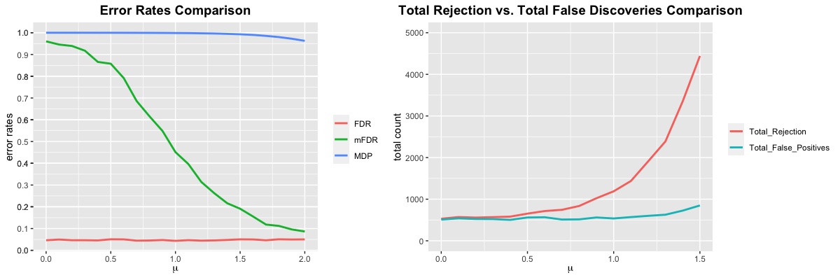
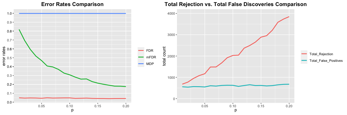
Figure 3: Error rates comparison between mFDR and FDR with varying signal strength and proportions.

References

- Bartroff (2014) Jay Bartroff. Multiple hypothesis tests controlling generalized error rates for sequential data. arXiv:1406.5933, 2014.
- Bartroff and Song (2013) Jay Bartroff and Jinlin Song. Sequential tests of multiple hypotheses controlling false discovery and nondiscovery rates. arXiv:1311.3350, 2013.
- Bartroff and Song (2016) Jay Bartroff and Jinlin Song. A rejection principle for sequential tests of multiple hypotheses controlling familywise error rates. Scandinavian Journal of Statistics, 43(1):3–19, 2016.
- Bashan et al. (2011) Eran Bashan, Gregory Newstadt, and Alfred O Hero. Two-stage multiscale search for sparse targets. IEEE Transactions on Signal Processing, 59(5):2331–2341, 2011.
- Benjamini and Bogomolov (2014) Yoav Benjamini and Marina Bogomolov. Selective inference on multiple families of hypotheses. Journal of the Royal Statistical Society: Series B (Statistical Methodology), 76(1):297–318, 2014.
- Benjamini and Heller (2007) Yoav Benjamini and Ruth Heller. False discovery rates for spatial signals. J. Amer. Statist. Assoc., 102:1272–1281, 2007. ISSN 0162-1459.
- Benjamini and Hochberg (1995) Yoav Benjamini and Yosef Hochberg. Controlling the false discovery rate: a practical and powerful approach to multiple testing. J. Roy. Statist. Soc. B, 57:289–300, 1995. ISSN 0035-9246.
- Berger (1985) James O Berger. Statistical decision theory and Bayesian analysis. Springer, 1985.
- Blanchard and Geman (2005) Gilles Blanchard and Donald Geman. Hierarchical testing designs for pattern recognition. Ann. Statist., 33:1155–1202, 2005.
- Bleicher et al. (2003) Konrad H Bleicher, Hans-Joachim Böhm, Klaus Müller, and Alexander I Alanine. Hit and lead generation: beyond high-throughput screening. Nature reviews Drug discovery, 2(5):369–378, 2003.
- Bloma et al. (2002) Paul E. Bloma, Shelby J. Fleischerb, and Zane Smilowitzb. Spatial and temporal dynamics of colorado potato beetle in fields with perimeter and spatially targeted insecticides. Environmental Entomology, 31(1):149–159, 2002.
- Cai and Sun (2009) T. Tony Cai and Wenguang Sun. Simultaneous testing of grouped hypotheses: Finding needles in multiple haystacks. J. Amer. Statist. Assoc., 104:1467–1481, 2009.
- Cai et al. (2007) T. Tony Cai, Jiashun Jin, and Mark G. Low. Estimation and confidence sets for sparse normal mixtures. Ann. Statist., 35(6):2421–2449, 2007. ISSN 0090-5364.
- Cai et al. (2019) T Tony Cai, Wenguang Sun, and Weinan Wang. Cars: Covariate assisted ranking and screening for large-scale two-sample inference (with discussion). Journal of the Royal Statistical Society: Series B (Statistical Methodology), 81:1–31, 2019.
- Cai and Sun (2017) Tony Cai and Wenguang Sun. Optimal screening and discovery of sparse signals with applications to multistage high throughput studies. Journal of the Royal Statistical Society: Series B (Statistical Methodology), 79(1):197–223, 2017.
- Copas (1974) J B Copas. On symmetric compound decision rules for dichotomies. Ann. Statist., 2:199–204, 1974.
- Cormack (1988) RM Cormack. Statistical challenges in the environmental sciences: a personal view. Journal of the Royal Statistical Society. Series A (Statistics in Society), pages 201–210, 1988.
- Djorgovski et al. (2012) S George Djorgovski, AA Mahabal, Ciro Donalek, Matthew J Graham, Andrew J Drake, Baback Moghaddam, and Mike Turmon. Flashes in a star stream: Automated classification of astronomical transient events. In E-Science (e-Science), 2012 IEEE 8th International Conference on, pages 1–8. IEEE, 2012.
- Dmitrienko et al. (2007) Alex Dmitrienko, Brian L Wiens, Ajit C Tamhane, and Xin Wang. Tree-structured gatekeeping tests in clinical trials with hierarchically ordered multiple objectives. Statistics in medicine, 26(12):2465–2478, 2007.
- Donoho and Jin (2004) David Donoho and Jiashun Jin. Higher criticism for detecting sparse heterogeneous mixtures. Ann. Statist., 32:962–994, 2004. ISSN 0090-5364.
- Efron (2004) Bradley Efron. Large-scale simultaneous hypothesis testing: the choice of a null hypothesis. J. Amer. Statist. Assoc., 99(465):96–104, 2004. ISSN 0162-1459. doi: 10.1198/016214504000000089. URL http://dx.doi.org/10.1198/016214504000000089.
- Efron (2008) Bradley Efron. Simultaneous inference: When should hypothesis testing problems be combined? Ann. Appl. Stat., 2:197–223, 2008.
- Efron et al. (2001) Bradley Efron, Robert Tibshirani, John D. Storey, and Virginia Tusher. Empirical Bayes analysis of a microarray experiment. J. Amer. Statist. Assoc., 96:1151–1160, 2001. ISSN 0162-1459.
- Genovese and Wasserman (2002) Christopher Genovese and Larry Wasserman. Operating characteristics and extensions of the false discovery rate procedure. J. R. Stat. Soc. B, 64:499–517, 2002. ISSN 1369-7412.
- Ghosh (1960) MN Ghosh. Bounds for the expected sample size in a sequential probability ratio test. Journal of the Royal Statistical Society. Series B (Methodological), pages 360–367, 1960.
- Goeman and Mansmann (2008) Jelle J. Goeman and Ulrich Mansmann. Multiple testing on the directed acyclic graph of gene ontology. Bioinformatics, 24(4):537–544, 2008.
- Haupt et al. (2011) J. Haupt, R. M. Castro, and R. Nowak. Distilled Sensing: Adaptive Sampling for Sparse Detection and Estimation. IEEE T. Inform. Theory, 57(9):6222–6235, 2011.
- Haupt et al. (2012) Jarvis Haupt, Richard G Baraniuk, Rui M Castro, and Robert D Nowak. Sequentially designed compressed sensing. In SSP, pages 401–404, 2012.
- Heller and Rosset (2019) Ruth Heller and Saharon Rosset. Optimal fdr control in the two-group model. arXiv preprint arXiv:1902.00892, 2019.
- James and Stein (1961) William James and Charles Stein. Estimation with quadratic loss. In Proceedings of the fourth Berkeley symposium on mathematical statistics and probability, volume 1, pages 361–379, 1961.
- Jin and Cai (2007) Jiashun Jin and T. Tony Cai. Estimating the null and the proportional of nonnull effects in large-scale multiple comparisons. J. Amer. Statist. Assoc., 102:495–506, 2007. ISSN 0162-1459.
- Johari et al. (2015) Ramesh Johari, Leo Pekelis, and David J Walsh. Always valid inference: Bringing sequential analysis to a/b testing. arXiv preprint arXiv:1512.04922, 2015.
- Liang and Nettleton (2010) Kun Liang and Dan Nettleton. A hidden markov model approach to testing multiple hypotheses on a tree-transformed gene ontology graph. Journal of the American Statistical Association, 105(492):1444–1454, 2010.
- Malloy and Nowak (2011) Matthew Malloy and Robert Nowak. Sequential analysis in high-dimensional multiple testing and sparse recovery. In Information Theory Proceedings (ISIT), 2011 IEEE International Symposium on, pages 2661–2665. IEEE, 2011.
- Malloy and Nowak (2014a) Matthew L Malloy and Robert D Nowak. Sequential testing for sparse recovery. IEEE Transactions on Information Theory, 60(12):7862–7873, 2014a.
- Malloy and Nowak (2014b) Matthew L Malloy and Robert D Nowak. Near-optimal adaptive compressed sensing. IEEE Transactions on Information Theory, 60(7):4001–4012, 2014b.
- Meinshausen and Rice (2006) Nicholai Meinshausen and John Rice. Estimating the proportion of false null hypotheses among a large number of independently tested hypotheses. Ann. Statist., 34:373–393, 2006.
- Meinshausen et al. (2009) Nicolai Meinshausen, Peter Bickel, John Rice, et al. Efficient blind search: Optimal power of detection under computational cost constraints. The Annals of Applied Statistics, 3(1):38–60, 2009.
- Müller et al. (2004) Peter Müller, Giovanni Parmigiani, Christian Robert, and Judith Rousseau. Optimal sample size for multiple testing: the case of gene expression microarrays. Journal of the American Statistical Association, 99(468):990–1001, 2004.
- Posch et al. (2009) Martin Posch, Sonja Zehetmayer, and Peter Bauer. Hunting for significance with the false discovery rate. Journal of the American Statistical Association, 104(486):832–840, 2009.
- Robbins (1951) Herbert Robbins. Asymptotically subminimax solutions of compound statistical decision problems. In Proceedings of the Second Berkeley Symposium on Mathematical Statistics and Probability, 1950, pages 131–148, Berkeley and Los Angeles, 1951. University of California Press.
- Roesch (1993) Francis A Roesch. Adaptive cluster sampling for forest inventories. Forest Science, 39(4):655–669, 1993.
- Rossell and Müller (2013) David Rossell and Peter Müller. Sequential stopping for high-throughput experiments. Biostatistics, 14(1):75–86, 2013.
- Rothman et al. (2010) Nathaniel Rothman, Montserrat Garcia-Closas, Nilanjan Chatterjee, Nuria Malats, Xifeng Wu, Jonine D Figueroa, Francisco X Real, David Van Den Berg, Giuseppe Matullo, Dalsu Baris, et al. A multi-stage genome-wide association study of bladder cancer identifies multiple susceptibility loci. Nature genetics, 42(11):978–984, 2010.
- Sarkar (2004) Sanat K Sarkar. Fdr-controlling stepwise procedures and their false negatives rates. J. Stat. Plan. Infer., 125(1):119–137, 2004.
- Sarkar et al. (2013) Sanat K Sarkar, Jingjing Chen, and Wenge Guo. Multiple testing in a two-stage adaptive design with combination tests controlling fdr. Journal of the American Statistical Association, 108(504):1385–1401, 2013.
- Satagopan et al. (2004) Jaya M Satagopan, ES Venkatraman, and Colin B Begg. Two-stage designs for gene–disease association studies with sample size constraints. Biometrics, 60(3):589–597, 2004.
- Siegmund (1985) David Siegmund. Sequential analysis: tests and confidence intervals. Springer Science & Business Media, 1985.
- Sun and Cai (2007) Wenguang Sun and T. Tony Cai. Oracle and adaptive compound decision rules for false discovery rate control. J. Amer. Statist. Assoc., 102:901–912, 2007. ISSN 0162-1459.
- Sun and Cai (2009) Wenguang Sun and T. Tony Cai. Large-scale multiple testing under dependence. J. R. Stat. Soc. B, 71:393–424, 2009.
- Sun and Wei (2015) Wenguang Sun and Zhi Wei. Hierarchical recognition of sparse patterns in large-scale simultaneous inference. Biometrika, 102:267–280, 2015.
- Sun et al. (2015) Wenguang Sun, Brian J Reich, T Tony Cai, Michele Guindani, and Armin Schwartzman. False discovery control in large-scale spatial multiple testing. Journal of the Royal Statistical Society: Series B (Statistical Methodology), 77(1):59–83, 2015.
- Thompson and Seber (1996) Steven K. Thompson and George A. Seber. Adaptive sampling. John Wiley & Sons, Inc., New York, NY, 1996.
- Victor and Hommel (2007) Anja Victor and Gerhard Hommel. Combining adaptive designs with control of the false discovery rate–a generalized definition for a global p-value. Biometrical Journal, 49(1):94–106, 2007.
- Wald (1945) Abraham Wald. Sequential tests of statistical hypotheses. The Annals of Mathematical Statistics, 16(2):117–186, 1945.
- Wald (1947) Abraham Wald. Sequential analysis. Wiley, New York, 1947.
- Wei and Hero (2013) Dennis Wei and Alfred O Hero. Multistage adaptive estimation of sparse signals. IEEE Journal of Selected Topics in Signal Processing, 7(5):783–796, 2013.
- Wei and Hero (2015) Dennis Wei and Alfred O Hero. Performance guarantees for adaptive estimation of sparse signals. IEEE Transactions on Information Theory, 61(4):2043–2059, 2015.
- Yekutieli (2008) Daniel Yekutieli. Hierarchical false discovery rate–controlling methodology. Journal of the American Statistical Association, 103(481):309–316, 2008.
- Zehetmayer et al. (2008) Sonja Zehetmayer, Peter Bauer, and Martin Posch. Optimized multi-stage designs controlling the false discovery or the family-wise error rate. Statistics in medicine, 27(21):4145–4160, 2008.
- Zhang et al. (1999) Ji-Hu Zhang, Thomas DY Chung, and Kevin R Oldenburg. A simple statistical parameter for use in evaluation and validation of high throughput screening assays. Journal of biomolecular screening, 4(2):67–73, 1999.