Nonintersecting Brownian bridges on the unit
circle with drift

Abstract.

Nonintersecting Brownian bridges on the unit circle form a determinantal stochastic process exhibiting random matrix statistics for large numbers of walkers. We investigate the effect of adding a drift term to walkers on the circle conditioned to start and end at the same position. For each return time $T<\pi^{2}$ we show that if the absolute value of the drift is less than a critical value then the expected total winding number is asymptotically zero. In addition, we compute the asymptotic distribution of total winding numbers in the double-scaling regime in which the expected total winding is finite. The method of proof is Riemann–Hilbert analysis of a certain family of discrete orthogonal polynomials with varying complex exponential weights. This is the first asymptotic analysis of such a class of polynomials. We determine asymptotic formulas and demonstrate the emergence of a second band of zeros by a mechanism not previously seen for discrete orthogonal polynomials with real weights.

1. Introduction

In 1962, Dyson [22] made the remarkable observation that the eigenvalues of an $n\times n$ GUE random matrix obey the same statistics as a certain process comprised of nonintersecting Brownian motions (NIBM). Since then, it has been shown that NIBM models give rise to a plethora of universal stochastic processes, including the sine, Airy, Pearcey, and tacnode processes [38, 39, 8, 20, 23, 28], which appear in a wide range of problems in probability and mathematical physics. In addition, NIBM models and related models of nonintersecting paths serve as tractable models for the study of subjects as diverse as transportation engineering [2], wetting and melting [24], polymers and random interfaces [35], Yang–Mills theory [26], dynamics of quantum systems [21], etc. Technically it is often easiest to study nonintersecting Brownian bridges, in which the starting and ending points of the Brownian paths are fixed.

A natural generalization is to consider nonintersecting Brownian bridges on the circle. This model was studied in depth recently by Wang and the second author in [33]. To be specific, they considered an ensemble of $n$ nonintersecting Brownian bridges on the unit circle ${\mathbb{T}}=\{e^{i\theta}|-\pi\leq\theta<\pi\}\subset\mathbb{C}$ with diffusion parameter $n^{-1/2}$, conditioned to begin at a common point at time $t=0$ and to end at the same common point at time $t=T>0$. We can summarize the global properties of that model as the number of particles $n\to\infty$ obtained in [33] as follows; see Figure 1. The asymptotic behavior of the particles as $n\to\infty$ depends on the return time $T$. In particular it is shown that there is a critical value $T_{c}=\pi^{2}$ of the return time $T$ separating the subcritical return times from the supercritical return times. In the subcritical case $T<\pi^{2}$, the particles do not have enough time to wrap around the circle and the asymptotic behavior is identical to nonintersecting Brownian bridges on the real line. In this case the limiting density of particles at any fixed time $t\in(0,T)$ converges to a properly rescaled semi-circle distribution and the boundary of the convex hull of the paths in space-time converges to an ellipse. In the supercritical case $T>\pi^{2}$, as $n\to\infty$ there is a nonvanishing probability that some particles wrap around the circle, and the distribution of the sum of the winding numbers of the particles converges to a discrete normal distribution. This case is considerably more complicated, and both the density of particles at fixed times and the boundary of the convex hull of the paths in space-time are expressed by elliptic functions.

In the current work we extend the model discussed above to nonintersecting Brownian bridges on ${\mathbb{T}}$ with a drift. For planar Brownian bridges, adding a drift to the Brownian motion has no effect, but for Brownian bridges on the unit circle the drift has the effect of encouraging particles to wrap around the circle. The analysis of [33] is based on the fact that the nonintersecting Brownian bridges on ${\mathbb{T}}$ form a determinantal process whose kernel can be expressed in terms of a system of discrete Gaussian orthogonal polynomials which may be studied asymptotically using Riemann–Hilbert methods. When a drift is added the structure of the determinantal process is the same, but now the discrete orthogonal polynomials we need to consider have a complex exponential weight. In general discrete orthogonal polynomials with complex weights are difficult to study asymptotically, and we are not aware of any such previous work.

Figure 1. Random walk simulations of a Dyson Brownian bridge on the circle with 24 walkers in the subcritical (left), critical (center), and supercritical (right) regimes.

Figure 2. Random walk simulations of a Dyson Brownian bridge on the circle with 24 walkers and total winding 3 (left) and 24 (right).

In the remainder of the introduction we define the model we study and present our results on winding numbers and orthogonal polynomials.

1.1. Definition of the model

Consider a Brownian motion on $\mathbb{R}$ with drift $\mu$ and diffusion parameter $\sigma$. By definition, the probability density for the particle to move from position $x$ to position $y$ in time $t$ is

(1.1) $$P_{\mathbb{R}}(x,y;t,\sigma,\mu)=\frac{1}{\sqrt{2\pi t}\sigma}\exp\left(-\frac{(y-x-t\mu)^{2}}{2t\sigma^{2}}\right).$$

Now consider a Brownian motion on the unit circle ${\mathbb{T}}$. We refer to a particle at $e^{i\varphi}$ as being at position $\varphi$ and use the principal value of the argument $-\pi\leq\varphi<\pi$. Taking into account that the particle can wrap around the circle multiple times, the transition probability density for a particle starting at $\varphi$ to move to $\theta$ in time $t$ is

(1.2) $$P_{\mathbb{T}}(\varphi,\theta;t,\sigma,\mu)=\frac{1}{\sqrt{2\pi t}\sigma}\sum_{k=-\infty}^{\infty}\exp\left(-\frac{(\theta-\varphi-t\mu+2k\pi)^{2}}{2t\sigma^{2}}\right).$$

We will consider an ensemble of $n$ Brownian motions on the unit circle and set the diffusion parameter to be $\sigma=n^{-1/2}$. We introduce a phase parameter $\tau$ and define

(1.3) $$P_{n}(\varphi,\theta;t,\mu,\tau):=\sqrt{\frac{n}{2\pi t}}\sum_{k=-\infty}^{\infty}\exp\left(-n\frac{(\theta-\varphi-t\mu+2k\pi)^{2}}{2t}+2\pi ik\tau\right).$$

This is no longer a probability density in general, but the parameter $\tau$ allows us to keep track of exactly how many times particles wraps around the circle. In particular,

(1.4) $$\mathbb{P}(\text{offset }\omega\,|\,\text{particle starts at }\varphi\text{ and ends at }\theta)=\int_{0}^{1}\frac{P_{n}(\varphi,\theta;t,\mu,\tau)e^{-2\pi i\omega\tau}}{P_{n}(\varphi,\theta;t,\mu,0)}d\tau.$$

This can be seen by noting the integral isolates the $k=\omega$ term in (1.3).

Now consider the transition probability density for $n$ such Brownian particles on ${\mathbb{T}}$ conditioned not to intersect. Let $A_{n}=\{a_{1},\dots,a_{n}\}$ and $B_{n}=\{b_{1},\dots,b_{n}\}$ be two sets of $n$ distinct points in ${\mathbb{T}}$ such that $-\pi\leq a_{1}<a_{2}<\dotsb<a_{n}<\pi$ and $-\pi\leq b_{1}<b_{2}<\dotsb<b_{n}<\pi$, and denote by $\mathcal{P}_{n}(A_{n},B_{n},t;\mu)$ the transition probability density of nonintersecting Brownian motions with the particles starting at the points $A_{n}$ and ending at the points $B_{n}$ after time $t$. Note that we do not require that the particle that started at point $a_{k}$ ends at point $b_{k}$, but only that it ends at point $b_{j}$ for some $j=1,\dots,n$. Introduce the notation

(1.5) $$\epsilon(n):=\begin{cases}0&\text{if $n$ is odd},\\ \frac{1}{2}&\text{if $n$ is even}.\end{cases}$$

We define the $n\times n$ determinant

(1.6) $$\mathcal{P}_{n}(A_{n},B_{n},t;\mu,\tau):=\det\bigg{(}P_{n}\big{(}a_{j},b_{k},t;\mu,\tau\big{)}\bigg{)}_{j,k=1}^{n}\,.$$

Following [33], we then have that the transition probability density function for the NIBM on ${\mathbb{T}}$ with starting points $A_{n}$ and ending points $B_{n}$ is given exactly by $\mathcal{P}_{n}(A_{n},B_{n},t;\mu,\epsilon(n))$.

At this point we fix a return time $T$ and take the limit as all of the starting and ending points go to zero. Then the joint density of the particles at a fixed time $t\in(0,T)$ is given by

(1.7) $$\lim_{\begin{subarray}{c}a_{1},\dots,a_{n}\to 0\\ b_{1},\dots,b_{n}\to 0\end{subarray}}\frac{\mathcal{P}_{n}(A_{n},\Theta_{n},t;\mu,\epsilon(n))\mathcal{P}_{n}(\Theta_{n},B_{n},t;\mu,\epsilon(n))}{\mathcal{P}_{n}(A_{n},B_{n},t;\mu,\epsilon(n))}\,,$$

where $\Theta_{n}=\{\theta_{1},\dotsc,\theta_{n}\}$ describes the locations of the $n$ particles at time $t$. It is not difficult to see that such a limit exists, and so that our model is well defined (see [33, Section 2.2]). This defines a model we denote as $\text{NIBM}^{\mu}_{0\to T}$.

The model $\text{NIBM}^{\mu}_{0\to T}$ is a determinantal process, meaning that for any fixed time $t\in(0,T)$, the correlation functions of the particles may be described by a particular determinantal formula. There exists some kernel function $K_{n}(x,y;t)$ such that the $k$-point correlation function for the positions of the particles at time $t$ is given by

(1.8) $$R_{0\to T}^{(n)}(\theta_{1},\dotsc,\theta_{k};t)=\det\left(K_{n}\left(\theta_{i},\theta_{j};t\right)\right)_{i,j=1}^{k}\,.$$

The kernel function $K_{n}\left(\theta_{i},\theta_{j};t\right)$ may be expressed in terms of orthogonal polynomials. Namely, let $p^{(T,\mu,\tau)}_{n,j}(x)$ be the monic polynomial of degree $j$ that satisfies

(1.9) $$\frac{1}{n}\sum_{x\in L_{n,\tau}}p^{(T,\mu,\tau)}_{n,j}(x)p^{(T,\mu,\tau)}_{n,k}(x)e^{-\frac{Tn}{2}(x^{2}-2i\mu x)}=h_{n,j}^{(T,\mu,\tau)}\delta_{jk}$$

for a sequence $\{h_{n,j}^{(T,\mu,\tau)}\}_{j=0}^{\infty}$ of normalizing constants, where the lattice $L_{n,\tau}$ is defined as

(1.10) $$L_{n,\tau}:=\left\{\frac{k+\tau}{n}\mid k\in\mathbb{Z}\right\}.$$

Also define the auxiliary function

(1.11) $$S_{j,a}(\varphi;T,\mu,\tau,n)\equiv S_{j,a}(\varphi):=\frac{1}{n}\sum_{x\in L_{n,\tau}}p_{n,j}^{(T,\mu,\tau)}(x)e^{-an(x^{2}-2i\mu x)/2}e^{i\varphi nx}.$$

The $\tau$-deformed correlation kernel is given by

(1.12) $$K_{n}(\varphi,\theta;t,T,\mu,\tau):=\frac{n}{2\pi}\sum_{j=0}^{n-1}\frac{1}{h_{n,j}^{(T,\mu,\tau)}}S_{j,T-t}(\varphi)S_{j,t}(-\theta),$$

and the correlation kernel in (1.8) is this kernel with $\tau=\epsilon(n)$:

(1.13) $$K_{n}\left(\theta_{i},\theta_{j};t\right):=K_{n}(\theta_{i},\theta_{j};t,T,\mu,\epsilon(n)).$$

Even though only the special case $\tau=\epsilon(n)$ in (1.12) defines a correlation kernel, the $\tau$-deformed kernel was useful in [33] for keeping track of the winding numbers in the model.

1.2. Distribution of winding numbers in $\text{NIBM}^{\mu}_{0\to T}$ 

In the process $\text{NIBM}^{\mu}_{0\to T}$, let $\mathcal{W}_{n}(T,\mu)$ be the total winding number of the $n$ particles. The distribution of $\mathcal{W}_{n}(T,\mu)$ can also be expressed in terms of the orthogonal polynomials (1.9). Introduce the Hankel determinant

(1.14) $$\mathcal{H}_{n}(T,\mu,\tau):=\det\left(\frac{1}{n}\sum_{x\in L_{n,\tau}}x^{j+k-2}e^{-\frac{Tn}{2}(x^{2}-2i\mu x)}dx\right)^{n}_{j,k=1}.$$

It is a standard result (see e.g. [10]) that $\mathcal{H}_{n}(T,\mu,\tau)$ is given in terms of the normalizing constants $h_{n,j}^{(T,\mu,\tau)}$ in (1.9) as

(1.15) $$\mathcal{H}_{n}(T,\mu,\tau):=\prod_{j=0}^{n-1}h_{n,j}^{(T,\mu,\tau)}.$$

The distribution of $\mathcal{W}_{n}(T,\mu)$ is given by

(1.16) $$\mathbb{P}(\mathcal{W}_{n}(T,\mu)=\omega)=e^{2\pi i\omega\epsilon(n)}\int_{0}^{1}\frac{\mathcal{H}_{n}(T,\mu,\tau)}{\mathcal{H}_{n}(T,\mu,\epsilon(n))}e^{-2\pi i\omega\tau}d\tau,\quad\omega\in\mathbb{Z}.$$

This formula is presented in [33, Equation (185)] in the case $\mu=0$, and its extension to general $\mu$ is straightforward.

We plot $\mathbb{P}(\mathcal{W}_{3}(1,\mu)=\omega)$, $\omega=0,...,3$ and $\mathbb{P}(\mathcal{W}_{6}(1,\mu)=\omega)$, $\omega=0,...,6$ in Figure 3.

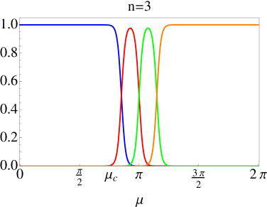
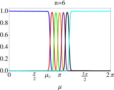
Figure 3. The probability of each winding number as a function of $\mu$ for $n=3$ and $n=6$. Left plot: $\mathbb{P}(\mathcal{W}_{3}(1,\mu)=\omega)$ for $\omega=0$ (blue), 1 (red), 2 (green), and 3 (orange). Right plot: $\mathbb{P}(\mathcal{W}_{6}(1,\mu)=\omega)$ for $\omega=0$ (blue), 1 (red), 2 (green), 3 (orange), 4 (purple), 5 (black), and 6 (cyan). The critical drift $\mu_{c}(1)\approx 2.4016$ is indicated, with $\mu_{c}(T)$ defined in (1.17).

We prove in Theorem 1.1 that for each $T\in(0,\pi^{2})$ there is a critical drift value $\mu_{c}(T)$ such that (asymptotically as $n\to\infty$) the expected winding is zero for $-\mu_{c}(T)<\mu<\mu_{c}(T)$. The exact formula for $\mu_{c}(T)$ is given in (1.17). From plots such as those in Figure 3, it is possible to formulate further conjectures concerning the expected winding number for other values of $\mu$ and $T$. For $\mu_{c}(T)<\mu<\frac{2\pi}{T}-\mu_{c}(T)$, there appears to be a transition region in which the expected winding number increases from 0 to $n$. After this, the expected winding number appears to be (asymptotically as $n\to\infty$) $n$ for $\frac{2\pi}{T}-\mu_{c}(T)<\mu<\frac{2\pi}{T}+\mu_{c}(T)$. This pattern appears to continue with the expected winding number increasing by $n$ when $\mu$ is increased by $\frac{2\pi}{T}$. This conjectured behavior is illustrated in Figure 4.

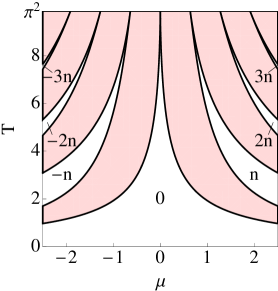
Figure 4. The conjectured expected winding number (in the large-$n$ limit) for different values of $\mu$ and $T$. The white regions have constant expected winding as indicated, while the transition regions are shaded. The figure could be extended arbitrarily far in either direction in $\mu$, but it is necessary to restrict $T$ to the interval $[0,\pi^{2}]$. Theorem 1.1 establishes the behavior in the zero-winding region, while Theorem 1.2 details the behavior at the edge of this region.

We now state our results on the winding numbers. Fix $T\in(0,\pi^{2})$ and define the critical drift

(1.17) $$\mu_{c}\equiv\mu_{c}(T):=\frac{\sqrt{\pi^{2}-T}}{T}-\frac{\log T}{2\pi}+\frac{\log(\pi-\sqrt{\pi^{2}-T})}{\pi}\quad(0<T<\pi^{2}).$$

For $|\mu|<\mu_{c}$, the asymptotic distribution of the random variable $\mathcal{W}_{n}(T,\mu)$, which represents the total winding number of the particles in $\text{NIBM}^{\mu}_{0\to T}$, is almost surely 1 in the limit $n\to\infty$.

Theorem 1.1 (Winding numbers in the subcritical regime).

Fix a return time $T\in(0,\pi^{2})$ and a drift $\mu$ such that $|\mu|<\mu_{c}(T)$, as defined in (1.17). Then there is a constant $c>0$ such that

(1.18) $$\mathbb{P}(\mathcal{W}_{n}(T,\mu)=\omega)=\begin{cases}1+\mathcal{O}\left(e^{-cn}\right),&\omega=0,\\ \mathcal{O}\left(e^{-cn}\right),&\omega\neq 0.\end{cases}$$

We will prove Theorem 1.1 in §4.4.

We now consider what we call the Hermite regime when $\mu$ is close to $\mu_{c}$ (but $T$ is still bounded away from $\pi^{2}$). Specifically, we fix a non-negative integer $k$ and choose $\mu$ so that

(1.19) $$\mu_{c}+\left(k-\frac{1}{2}\right)\frac{\log n}{2\pi n}<\mu\leq\mu_{c}+\left(k+\frac{1}{2}\right)\frac{\log n}{2\pi n}.$$

The continuous Hermite polynomials will play an important role in the analysis in this situation.

Theorem 1.2 (Winding numbers in the Hermite regime).

Fix a return time $T\in(0,\pi^{2})$ and a non-negative integer $k$, and choose $\mu$ satisfying (1.19). Then

(1.20) $$\mathbb{P}(\mathcal{W}_{n}(T,\mu)=\omega)=\begin{cases}\displaystyle\frac{F_{k-1}^{-1}}{1+F_{k}+F_{k-1}^{-1}}+\mathcal{O}\left(\frac{1}{n}\right),&\omega=k-1,\\ \displaystyle\frac{1}{1+F_{k}+F_{k-1}^{-1}}+\mathcal{O}\left(\frac{1}{n}\right),&\omega=k,\\ \displaystyle\frac{F_{k}}{1+F_{k}+F_{k-1}^{-1}}+\mathcal{O}\left(\frac{1}{n}\right),&\omega=k+1,\vspace{.1in}\\ \displaystyle\mathcal{O}\left(\frac{1}{n}\right),&\text{otherwise},\end{cases}$$

where

(1.21) $$F_{j}\equiv F_{j}(T,\mu,n):=\begin{cases}\displaystyle\frac{j!}{2^{j+1}\sqrt{\pi}}\left(\frac{T}{(2\pi)^{3/2}(\pi^{2}-T)^{1/4}}\right)^{2j+1}\frac{e^{2\pi n(\mu-\mu_{c}(T))}}{n^{j+(1/2)}},&j\in\mathbb{N},\\ 0,&j=-1.\end{cases}$$

Here $F_{k-1}=o(1)$ except at $\mu=\mu_{c}+(k-\frac{1}{2})\frac{\log n}{2\pi n}$, and $F_{k}=o(1)$ except at $\mu=\mu_{c}+(k+\frac{1}{2})\frac{\log n}{2\pi n}$.

Theorem 1.2 is proved in §5.5.

Remark 1.

In addition to information about the winding number, it is also natural to ask about the asymptotic distribution of particles in $\text{NIBM}^{\mu}_{0\to T}$ . Using the kernel (1.13), one can approach global questions about the asymptotic distribution of particles at any fixed time or the limiting shape of the complex hull of the paths in space-time, as well as local questions about the statistics of particles in various scaling limits. For $\mu=0$, these questions were answered in [32, 33] by rewriting (1.13) as a double contour integral, using the asymptotic expansion of the orthogonal polynomials and their discrete Cauchy transforms obtained from Riemann–Hilbert analysis, and performing classical steepest-descent analysis on the double contour integrals. This approach should also apply for general $\mu$, and for $T<\pi^{2}$ and $|\mu|$ small enough, the approach of [33] can be followed exactly to obtain identical results. Namely, the paths collect inside an ellipse in space-time, at any fixed time $t$ the density of particles converges to a semi-circle, and there are local scaling limits to the sine process in the bulk and to the Airy process at the edge. However, for certain values of $\mu<\mu_{c}(T)$, we have a technical difficulty in carrying out this program. The reason is that, although the asymptotic formulas for the orthogonal polynomials $p^{(T,\mu,\tau)}_{n,n}(z)$ are simple, see Theorem 1.3 below, the asymptotic formulas for their discrete Cauchy transforms become more complicated in certain regions of the complex plane.

1.3. Discrete orthogonal polynomials with complex weight

We prove our results on winding numbers by asymptotically analyzing the (meromorphic) Riemann–Hilbert problem associated to the discrete orthogonal polynomials (1.9). Orthogonal polynomials are a powerful tool for asymptotic analysis of nonintersecting particle systems (see the survey article [29] for an overview). A non-exhaustive list of applications includes the analysis of nonintersecting random walks by orthogonal polynomials on the unit circle [1], discrete Krawtchouk and Charlier polynomials [30], and Stieltjes–Wigert polynomials [5]; nonintersecting Brownian motions on the line with multiple starting and ending points by multiple orthogonal polynomials [16]; nonintersecting Brownian bridges on the line with distinct drifts by biorthogonal Stieltjes–Wigert polynomials [37]; and widths of nonintersecting Brownian bridges by Hermite polynomials and their discrete Gaussian counterparts [4].

Discrete Gaussian orthogonal polynomials with a real weight are the main tool in the analysis of the zero-drift version of the process $\text{NIBM}^{\mu}_{0\to T}$ [33]. Discrete orthogonal polynomials display some remarkably different properties from their continuous analogues. One well-known example for real weights is saturation of zeros, which follows from the upper limit on the density of zeros due to the fact that there can be at most one zero between any two lattice points on which the weight is supported (see, e.g., [3, 31, 33]). Saturation occurs in the zero-drift case for $T>\pi^{2}$ and corresponds to the two edges of the sea of walkers touching at $\theta=\pi$ (see the third panel in Figure 1). Saturation also plays a role for $T>\pi^{2}$ when the drift is non-zero, although that is beyond the scope of this paper. Instead, we describe and analyze a new band formation phenomenon. For sufficiently small drift values the locus of accumulating zeros is a single band, but at the critical value $\mu_{c}(T)$ zeros also appear at a new point (each new zero corresponds to an increase in the expected winding number). Similar behavior arises in the so-called birth of a cut for random matrix eigenvalues, which has been studied using continuous orthogonal polynomials with a real but non-convex weight [14, 7, 34]. In the Riemann–Hilbert analysis it is necessary to insert a local parametrix built from continuous Hermite polynomials and modify the outer parametrix. This construction also arises for the solitonic edge of an oscillatory zone in the solution of the small-dispersion Korteweg–de Vries equation [15], for a librational-rotational transition region in the solution of the small-dispersion sine-Gordon equation [11], and at the edge of the pole region for rational Painlevé-II functions [13].

This new phenomenon arises from the particular combination of a complex weight and discrete orthogonal polynomials. No band opens at a single point in the zero-drift problem analyzed by discrete Gaussian orthogonal polynomials with a real weight [33]. To see that this behavior also depends on the fact that we are using discrete orthogonal polynomials, consider the continuous analogue of (1.9). That is, let $H_{n,k}^{(T,\mu)}(x)$ be the monic polynomial of degree $k$ satisfying

(1.22) $$\int_{\mathbb{R}}H_{n,k}^{(T,\mu)}(x)H_{n,j}^{(T,\mu)}(x)e^{-\frac{nT}{2}(x^{2}-2i\mu x)}dx=h_{n,k}^{(T,\mu)}\delta_{jk},$$

for a sequence $\{h_{n,k}^{(T,\mu)}\}_{k=0}^{\infty}$ of normalizing constants. For $\mu=0$ these are the rescaled monic versions of the classical Hermite polynomials. For general $\mu$, we can complete the square in the exponent to obtain

(1.23) $$\int_{\mathbb{R}}H_{n,k}^{(T,\mu)}(x)H_{n,j}^{(T,\mu)}(x)e^{-\frac{nT}{2}(x-i\mu)^{2}}dx=e^{nT\mu^{2}/2}h_{n,k}^{(T,\mu)}\delta_{jk},$$

or equivalently

(1.24) $$\int_{\mathbb{R}-i\mu}H_{n,k}^{(T,\mu)}(x+i\mu)H_{n,j}^{(T,\mu)}(x+i\mu)e^{-\frac{nT}{2}x^{2}}dx=e^{nT\mu^{2}/2}h_{n,k}^{(T,\mu)}\delta_{jk}.$$

Using Cauchy’s theorem, the contour of integration can be deformed back to the real line, giving the orthogonality condition for $H_{n,k}^{(T,0)}(x)$. We thus find that the orthogonal polynomials (1.22) with complex weight are related to the ones with real weight ($\mu=0$) simply by a shift:

(1.25) $$H_{n,k}^{(T,\mu)}(x)\equiv H_{n,k}^{(T,0)}(x-i\mu).$$

Therefore the complexified weight cannot lead to new behavior for the continuous Hermite polynomials. This argument relies on a deformation of the contour of integration, which clearly is not possible for the discrete orthogonal polynomials (1.9). For discrete orthogonal polynomials with the complexified weight we will show in Theorem 1.3 an analogous relation holds, but only for sufficiently small drift (see (1.31)). The asymptotics of $p^{(T,\mu,\tau)}_{n,n}(z)$ near the critical drift are given in Theorem 1.4.

The current work is, to the best of our knowledge, the first investigation of discrete orthogonal polynomials with a complex weight. However, there are examples of asymptotic studies of continuous orthogonal polynomials with complex weights, including a weight supported on a real compact interval [17] and on arcs in the complex plane [27]. In both cases band splitting was studied but the birth of a new band at a point was not observed. A case where a new band appears at a point is the analysis of orthogonal polynomials on the unit circle to study rational Painlevé-II solutions [6].

Below we describe the asymptotic behavior of the polynomials $p^{(T,\mu,\tau)}_{n,n}(z)$ for $0<T<\pi^{2}$ as $n\to\infty$ in various regions of the complex plane separately in the cases $\mu<\mu_{c}(T)$ and $\mu\approx\mu_{c}(T)$. In this paper we do not consider non-scaling regimes when $\mu>\mu_{c}(T)$, which are considerably more complicated and can involve elliptic functions. We first introduce a few notations. Set

(1.26) $$g_{0}(z):=\frac{T}{4}z\left(z-\sqrt{z^{2}-\frac{4}{T}}\right)-\log\left(z-\sqrt{z^{2}-\frac{4}{T}}\right)-\frac{1}{2}+\log\frac{2}{T},\qquad\ell_{0}:=-1-\log T,$$

where the principal branches of the logarithm and square root are chosen. These are the $g$-function and Lagrange multiplier associated to the rescaled continuous Hermite polynomials [18] and are also used for the Brownian bridge on the circle when $\mu=0$ and $0<T<\pi^{2}$ [33]. Now we define the $g$-function and the Lagrange multiplier for nonzero $\mu$ as

(1.27) $$g(z):=g_{0}(z-i\mu),\quad\ell:=\ell_{0}-\frac{T}{2}\mu^{2}.$$

Define the function $\gamma(z)$ to be

(1.28) $$\gamma(z):=\left(\frac{z-a}{z-b}\right)^{1/4},\quad\textrm{where}\quad a:=-\frac{2}{\sqrt{T}}+i\mu,\quad b:=\frac{2}{\sqrt{T}}+i\mu,$$

with a cut on the horizontal line segment $(a,b)$, taking the branch such that $\gamma(\infty)=1$. Since both $g(z)$ and $\gamma(z)$ have cuts on $(a,b)$, for $z\in(a,b)$ we define $g_{\pm}(z)$ and $\gamma_{\pm}(z)$ to be the limiting values of these functions as $z$ approaches $(a,b)$ from above (respectively, below) the interval.

Theorem 1.3 (Orthogonal polynomial asymptotics in the subcritical regime).

Let $T\in(0,\pi^{2})$ be fixed, and $\mu\in\mathbb{R}$ with $|\mu|<\mu_{c}(T)$, where $\mu_{c}(T)$ is defined in (1.17).

1. Let $z$ be bounded away from the band $(a,b)$. As $n\to\infty$, the polynomial $p^{(T,\mu,\tau)}_{n,n}(z)$ satisfies

   (1.29) $$p^{(T,\mu,\tau)}_{n,n}(z)=e^{ng(z)}\left(\frac{\gamma(z)+\gamma(z)^{-1}}{2}\right)\left(1+\mathcal{O}(n^{-1})\right),$$

   and the error is uniform on subsets of $\mathbb{C}$ that are bounded away from the interval $(a,b)$.

2. Let $z$ be in a compact subset of the band $(a,b)$. As $n\to\infty$, the polynomial $p^{(T,\mu,\tau)}_{n,n}(z)$ satisfies

   (1.30) $$p^{(T,\mu,\tau)}_{n,n}(z)=\left[e^{ng_{+}(z)}\left(\frac{\gamma_{+}(z)+\gamma_{+}(z)^{-1}}{2}\right)+e^{ng_{-}(z)}\left(\frac{\gamma_{-}(z)+\gamma_{-}(z)^{-1}}{2}\right)\right]\left(1+\mathcal{O}(n^{-1})\right),$$

   and the error is uniform on compact subsets of $(a,b)$.

Theorem 1.3 is proved in §4.5.

Remark 2.

Notice that the functions involved in Theorem 1.3 are the same ones involved in the asymptotics of $p^{(T,\mu,\tau)}_{n,n}(z)$ with $\mu=0$, but shifted by $i\mu$. Indeed, this theorem implies that as $n\to\infty$,

(1.31) $$p^{(T,\mu,\tau)}_{n,n}(z)={p^{(T,0,\tau)}_{n,n}(z-i\mu)}(1+\mathcal{O}(n^{-1}))=H_{n,n}^{(T,\mu)}(z)(1+\mathcal{O}(n^{-1})),$$

provided $0<T<\pi^{2}$ and $|\mu|<\mu_{c}$. In Theorem 1.4, we see that this no longer holds when $\mu$ is scaled close to $\mu_{c}$.

We introduce the function

(1.32) $$D(z;\mu,T):=\frac{\sqrt{T}}{2i}(z-i\mu+R(z;\mu,T)),$$

where

(1.33) $$R(z;\mu,T):=((z-a(\mu,T))(z-b(\mu,T)))^{1/2}$$

is chosen with branch cut $[a,b]$ so that $R(z)=z+\mathcal{O}(1)$ as $z\to\infty$. Also introduce the point on the imaginary axis

(1.34) $$\widetilde{z}_{c}(\mu,T):=i\mu-\frac{2i}{T}\sqrt{\pi^{2}-T},$$

the constant

(1.35) $$\alpha_{\infty}:=\frac{-i}{D(\widetilde{z}_{c})}=\frac{\sqrt{\pi^{2}-T}+\pi}{\sqrt{T}}i,$$

and the function

(1.36) $$\alpha(z;\mu,T):=i\frac{D(\widetilde{z}_{c};\mu,T)-D(z;\mu,T)}{1+D(\widetilde{z}_{c};\mu,T)D(z;\mu,T)}.$$

Finally, let $\mathfrak{h}_{k}(\zeta)$ be the (orthonormal) Hermite polynomial of degree $k$, where $k$ is a non-negative integer. The Hermite polynomials satisfy

(1.37) $$\int_{\mathbb{R}}\mathfrak{h}_{j}(\zeta)\mathfrak{h}_{k}(\zeta)e^{-z^{2}}d\zeta=\delta_{jk},$$

and $\mathfrak{h}_{0}(\zeta)\equiv 1$. Denote the leading coefficient by $\kappa_{k}$:

(1.38) $$\mathfrak{h}_{k}(\zeta)=\kappa_{k}\zeta^{k}+\mathcal{O}(\zeta^{k-1}),\quad\kappa_{k}:=\frac{2^{k/2}}{\pi^{1/4}\sqrt{k!}}.$$

Theorem 1.4 (Orthogonal polynomials in the Hermite regime).

Fix $T\in(0,\pi^{2})$ and a non-negative integer $k$, and choose $\mu$ satisfying (1.19).

1. Let $z$ be bounded away from the band $(a,b)$ and the point $\widetilde{z}_{c}(\mu,T)$. As $n\to\infty$, the polynomial $p^{(T,\mu,\tau)}_{n,n}(z)$ satisfies

   (1.39) $$p^{(T,\mu,\tau)}_{n,n}(z)=e^{ng(z)}\left(\frac{\alpha(z)}{\alpha_{\infty}}\right)^{k}\left(\frac{\gamma(z)+\gamma(z)^{-1}}{2}\right)\left(1+\mathcal{O}\left(\frac{e^{2\pi n(\mu-\mu_{c})}}{n^{k+\frac{1}{2}}}\right)+\mathcal{O}\left(\frac{n^{k-\frac{1}{2}}}{e^{2\pi n(\mu-\mu_{c})}}\right)\right),$$

   and the error is uniform on subsets of $\mathbb{C}$ which are bounded away from the interval $(a,b)$ and the point $\widetilde{z}_{c}(\mu,T)$.

2. Let $z$ be in a compact subset of the band $(a,b)$. As $n\to\infty$, the polynomial $p^{(T,\mu,\tau)}_{n,n}(z)$ satisfies

   (1.40) $$\begin{split}p^{(T,\mu,\tau)}_{n,n}(z)=&\left[\frac{\alpha_{+}(z)^{k}}{\alpha_{\infty}^{k}}e^{ng_{+}(z)}\left(\frac{\gamma_{+}(z)+\gamma_{+}(z)^{-1}}{2}\right)+\frac{\alpha_{-}(z)^{k}}{\alpha_{\infty}^{k}}e^{ng_{-}(z)}\left(\frac{\gamma_{-}(z)+\gamma_{-}(z)^{-1}}{2}\right)\right]\\ &\times\left(1+\mathcal{O}\left(\frac{e^{2\pi n(\mu-\mu_{c})}}{n^{k+\frac{1}{2}}}\right)+\mathcal{O}\left(\frac{n^{k-\frac{1}{2}}}{e^{2\pi n(\mu-\mu_{c})}}\right)\right),\end{split}$$

   and the error is uniform on compact subsets of $(a,b)$.

3. There is a neighborhood $\mathbb{D}_{\widetilde{z}_{c}}$ of $\widetilde{z}_{c}$ and a local coordinate $W(z)$ (defined in (5.8)) such that, for $z\in\mathbb{D}_{\widetilde{z}_{c}}$,

   (1.41) $$\begin{split}p^{(T,\mu,\tau)}_{n,n}(z)=&e^{ng(z)}\left(\frac{\alpha(z)}{\alpha_{\infty}W(z)}\right)^{k}\left(\frac{\gamma(z)+\gamma(z)^{-1}}{2}\right)\frac{\mathfrak{h}_{k}(n^{1/2}W(z))}{\kappa_{k}n^{k/2}}\\ &\times\left(1+\mathcal{O}\left(\frac{e^{2\pi n(\mu-\mu_{c})}}{n^{k+\frac{1}{2}}}\right)+\mathcal{O}\left(\frac{n^{k-\frac{1}{2}}}{e^{2\pi n(\mu-\mu_{c})}}\right)\right).\end{split}$$

Theorem 1.4 is proved in §5.6.

Remark 3.

The complicated form of the error term arises from the fact that, although $\mu$ is a continuous parameter, the asymptotic behavior in the Hermite regime is naturally discretized in the sense that the choice of interval in (1.19) determines the qualitative behavior. This discretization is visually evident for the winding numbers in Figure 3, and for the orthogonal polynomials it manifests itself in the number of outlying zeros (see Remark 4). Simply keeping the leading-order terms as we have done in Theorem 1.4 has the advantage of giving simpler formulas with more straightforward derivations. However, it necessarily gives non-uniform errors due to the different behavior on different intervals. In fact, the first error term is actually $\mathcal{O}(1)$ if $\mu=\mu_{c}+(k+\frac{1}{2})\frac{\log n}{2\pi n}$ and the second error term is $\mathcal{O}(1)$ if $\mu=\mu_{c}+(k-\frac{1}{2})\frac{\log n}{2\pi n}$. A uniform expression can be obtained if desired using the analysis in this paper by keeping additional terms, and we carry out this procedure completely in Theorems 1.2 and 1.6.

Remark 4.

Equation (1.41) shows that $p^{(T,\mu,\tau)}_{n,n}(z)$ asymptotically has $k$ zeros (possibly counting multiplicity) near $\widetilde{z}_{c}$ in the Hermite regime. Indeed, $\alpha(z)$ and $W(z)$ both have simple zeros at $\widetilde{z}_{c}$ (see (5.53)), so the term

$$e^{ng(z)}\left(\frac{\alpha(z)}{\alpha_{\infty}W(z)}\right)^{k}\left(\frac{\gamma(z)+\gamma(z)^{-1}}{2}\right)$$

is well-defined and non-zero in a neighborhood of $\widetilde{z}_{c}$. Furthermore, $\mathfrak{h}_{k}$ has exactly $k$ simple zeros on the real line, and $W$ is a conformal map in this neighborhood, so $\mathfrak{h}_{k}(n^{1/2}W(z))$ also has $k$ simple zeros in a neighborhood of $\widetilde{z}_{c}$ for $n$ large enough.

Remark 5.

In part (b) of Theorems 1.3 and 1.4 all of the functions involved in the asymptotic formulas have analytic extensions into a neighborhood of the band $(a,b)$, so these asymptotics can be extended to a neighborhood of compact subsets of $(a,b)$.

Remark 6.

Neither Theorem 1.3 nor 1.4 describe the asymptotics behavior of the orthogonal polynomials close to the band endpoints $a$ and $b$. Near these points the asymptotic behavior is described by Airy functions. We omit this analysis, which is standard, from the current paper.

The orthogonal polynomials (1.9) satisfy the three term recurrence equation (see [36])

(1.42) $$xp^{(T,\mu,\tau)}_{n,k}(x)=p^{(T,\mu,\tau)}_{n,k+1}(x)+\beta^{(T,\mu,\tau)}_{n,k}p^{(T,\mu,\tau)}_{n,k}(x)+\left(\gamma^{(T,\mu,\tau)}_{n,k}\right)^{2}p^{(T,\mu,\tau)}_{n,k-1}(x)\,,$$

where $\{\beta^{(T,\mu,\tau)}_{n,j}\}_{j=0}^{\infty}$ is a sequence of constants, and

(1.43) $$\left(\gamma^{(T,\mu,\tau)}_{n,j}\right)^{2}:=\frac{h^{(T,\mu,\tau)}_{n,j}}{h^{(T,\mu,\tau)}_{n,j-1}}.$$

The asymptotic behavior of the recurrence coefficients and normalizing constants is presented in the last two theorems.

Theorem 1.5 (Normalizing constants and recurrence coefficients in the subcritical regime).

Let $T\in(0,\pi^{2})$ be fixed, and $\mu\in\mathbb{R}$ with $|\mu|<\mu_{c}(T)$. The normalizing constants and recurrence coefficients satisfy the following asymptotics as $n\to\infty$.

(1.44) $$h^{(T,\mu,\tau)}_{n,n}=\frac{2\pi}{T^{n+\frac{1}{2}}e^{n(\frac{1}{2}T\mu^{2}+1)}}(1+\mathcal{O}(n^{-1})),\qquad\left(h^{(T,\mu,\tau)}_{n,n-1}\right)^{-1}=\frac{T^{n-\frac{1}{2}}e^{n(\frac{1}{2}T\mu^{2}+1)}}{2\pi}(1+\mathcal{O}(n^{-1})),$$

(1.45) $$\beta^{(T,\mu,\tau)}_{n,n-1}=i\mu+\mathcal{O}(n^{-1}),\qquad\left(\gamma^{(T,\mu,\tau)}_{n,n}\right)^{2}=\frac{1}{T}+\mathcal{O}(n^{-1}).$$

Theorem 1.5 is proved in §4.5.

We now define

(1.46) $$\lambda\equiv\lambda(T):=i\frac{\pi+\sqrt{\pi^{2}-T}+i\sqrt{T}}{\pi-\sqrt{\pi^{2}-T}-i\sqrt{T}}$$

and

(1.47) $$G_{j}\equiv G_{j}(T,\mu,\tau,n):=(-1)^{n+1}F_{j}(T,\mu,n)e^{2\pi i\tau},\quad j\in\{-1\}\cup\mathbb{N}.$$

Then the asymptotic behavior of the normalization constants in the Hermite regime is as follows.

Theorem 1.6 (Normalizing constants and recurrence coefficients in the Hermite regime).

Fix $T\in(0,\pi^{2})$ and a non-negative integer $k$, and choose $\mu$ satisfying (1.19). Then

(1.48) $$h_{n,n}^{(T,\mu,\tau)}=\left\{\begin{aligned} &\frac{2\pi}{T^{n+\frac{1}{2}}e^{n(\frac{1}{2}T\mu^{2}+1)}}\left(1+\frac{2\pi}{\sqrt{T}}\frac{G_{k}}{1+G_{k}}\lambda+\frac{2\pi}{\sqrt{T}}\frac{G_{k-1}^{-1}}{1+G_{k-1}^{-1}}\lambda^{-1}+\mathcal{O}(n^{-1})\right)\alpha_{\infty}^{-2k},\ &{\rm for}\ k>0,\\ &\frac{2\pi}{T^{n+\frac{1}{2}}e^{n(\frac{1}{2}T\mu^{2}+1)}}\left(1+\frac{2\pi}{\sqrt{T}}\frac{G_{k}}{1+G_{k}}\lambda+\mathcal{O}(n^{-1})\right)\alpha_{\infty}^{-2k},\ &{\rm for}\ k=0,\end{aligned}\right.$$

(1.49) $$\begin{split}&\left(h_{n,n-1}^{(T,\mu,\tau)}\right)^{-1}=\\ &\,\,\,\,\left\{\begin{aligned} &\frac{T^{n-\frac{1}{2}}e^{n(\frac{1}{2}T\mu^{2}+1)}}{2\pi}\left(1+\frac{2\pi}{\sqrt{T}}\frac{G_{k}}{1+G_{k}}\lambda^{-1}+\frac{2\pi}{\sqrt{T}}\frac{G_{k-1}^{-1}}{1+G_{k-1}^{-1}}\lambda+\mathcal{O}(n^{-1})\right)\alpha_{\infty}^{2k},\ &{\rm for}\ k>0,\\ &\frac{T^{n-\frac{1}{2}}e^{n(\frac{1}{2}T\mu^{2}+1)}}{2\pi}\left(1+\frac{2\pi}{\sqrt{T}}\frac{G_{k}}{1+G_{k}}\lambda^{-1}+\mathcal{O}(n^{-1})\right)\alpha_{\infty}^{2k},\ &{\rm for}\ k=0,\\ \end{aligned}\right.\end{split}$$

(1.50) $$\left(\gamma^{(T,\mu,\tau)}_{n,j}\right)^{2}=\frac{1}{T}\left(1+\frac{2\pi}{\sqrt{T}}\left(\frac{G_{k}}{1+G_{k}}+\frac{G_{k-1}^{-1}}{1+G_{k-1}^{-1}}\right)(\lambda+\lambda^{-1})\right.\\ \left.+\frac{4\pi^{2}}{T}\left(\left(\frac{G_{k}}{1+G_{k}}\right)^{2}+\left(\frac{G_{k-1}^{-1}}{1+G_{k-1}^{-1}}\right)^{2}\right)+\mathcal{O}(n^{-1})\right).$$

Here $G_{k-1}^{-1}=o(1)$ except at $\mu=\mu_{c}+(k-\frac{1}{2})\frac{\log n}{2\pi n}$, and $G_{k}=o(1)$ except at $\mu=\mu_{c}+(k+\frac{1}{2})\frac{\log n}{2\pi n}$.

If desired, the asymptotic behavior of $\beta_{n,n-1}^{(T,\mu,\tau)}$ can also be extracted from the analysis in this paper, although we do not write down the lengthy but straightforward derivation. Theorem 1.6 is proved in §5.6.

1.4. Outline and notation

From (1.16), the distribution of winding numbers is expressed in terms of the Hankel determinant $\mathcal{H}_{n}(T,\mu,\tau)$. We start in §2 by representing the logarithm of this determinant as an integral involving the coefficient of the $x^{n-1}$ term of the orthogonal polynomial $p_{n,n}^{(T,\mu,\tau)}(x)$. This connection allows us to use asymptotic analysis of the orthogonal polynomials to obtain information on the winding numbers. In §3 we pose the Riemann–Hilbert problem encoding the discrete orthogonal polynomials and carry out several standard steps in the nonlinear steepest-descent analysis, namely interpolation of the poles, introduction of the $g$-function, and opening of lenses. In §4 we complete the analysis in the subcritical case and compute the winding numbers and orthogonal polynomial asymptotics for $|\mu|<\mu_{c}$. Finally, in §5 we consider the double-scaling limit $n\to\infty$, $\mu\to\mu_{c}$ and compute the winding numbers and orthogonal polynomial asymptotics in the Hermite regime.

Notation. With the exception of

(1.51) $$\mathbb{I}:=\begin{bmatrix}1&0\\ 0&1\end{bmatrix},\quad\sigma_{1}:=\begin{bmatrix}0&1\\ 1&0\end{bmatrix},\quad\sigma_{3}:=\begin{bmatrix}1&0\\ 0&-1\end{bmatrix},$$

matrices are denoted by bold capital letters. The non-negative integers are denoted by $\mathbb{N}$. We denote the $(jk)$th entry of a matrix ${\bf M}$ by $[{\bf M}]_{jk}$. In reference to a smooth, oriented contour $\Sigma$, for $z\in\Sigma$ we denote by $f_{+}(z)$ (respectively, $f_{-}(z)$) the non-tangential limit of $f(\zeta)$ as $\zeta$ approaches $\Sigma$ from the left (respectively, the right).

2. Integral representation for the Hankel determinant $\mathcal{H}_{n}(T,\mu,\tau)$

We begin by deriving a differential identity satisfied by the Hankel determinant $\mathcal{H}_{n}(T,\mu,\tau)$. Introduce the notation for the coefficients of the orthogonal polynomials

(2.1) $$p^{(T,\mu,\tau)}_{n,k}(x)=x^{k}+\sum_{j=0}^{k-1}c^{(T,\mu,\tau)}_{n,k,j}x^{j}.$$

We then have the following proposition.

Proposition 2.1.

The Hankel determinant $\mathcal{H}_{n}(T,\mu,\tau)$ satisfies the differential equation

(2.2) $$\frac{\partial}{\partial\tau}\log\mathcal{H}_{n}(T,\mu,\tau)=inT\mu+Tc^{(T,\mu,\tau)}_{n,n,n-1}.$$

Proof.

By (1.15),

(2.3) $$\frac{\partial}{\partial\tau}\log\mathcal{H}_{n}(T,\mu,\tau)=\sum_{j=0}^{n-1}\frac{\frac{\partial}{\partial\tau}h^{(T,\mu,\tau)}_{n,j}}{h^{(T,\mu,\tau)}_{n,j}}.$$

Therefore we compute $\frac{\partial}{\partial\tau}h^{(T,\mu,\tau)}_{n,k}$. We have

(2.4) $$h^{(T,\mu,\tau)}_{n,k}=\frac{1}{n}\sum_{\ell\in\mathbb{Z}}p^{(T,\mu,\tau)}_{n,k}\left(\frac{\ell+\tau}{n}\right)^{2}e^{-\frac{T}{2n}\left(\ell+\tau\right)^{2}}e^{iT\mu\left(\ell+\tau\right)}.$$

Writing $x_{\ell}=\frac{\ell+\tau}{n}$ and taking the derivative with respect to $\tau$ gives

(2.5) $$\frac{\partial}{\partial\tau}h^{(T,\mu,\tau)}_{n,k} =\frac{1}{n}\sum_{\ell\in\mathbb{Z}}\left[\frac{2}{n}p^{(T,\mu,\tau)}_{n,k}(x_{\ell})\left(\frac{\partial}{\partial\tau}p^{(T,\mu,\tau)}_{n,k}(x_{\ell})\right)-Tx_{\ell}+iT\mu\right]e^{-\frac{T}{2n}\left(\ell+\tau\right)^{2}}e^{iT\mu\left(\ell+\tau\right)}$$

$$=\frac{1}{n}\sum_{x\in L_{n,\tau}}\left[\frac{2}{n}p^{(T,\mu,\tau)}_{n,k}(x)\left(\frac{\partial}{\partial\tau}p^{(T,\mu,\tau)}_{n,k}(x)\right)+(iT\mu-Tx)p^{(T,\mu,\tau)}_{n,k}(x)^{2}\right]e^{-\frac{nT}{2}(x^{2}-2i\mu x)}$$

$$=iT\mu h^{(T,\mu,\tau)}_{n,k}-\frac{T}{n}\sum_{x\in L_{n,\tau}}xp^{(T,\mu,\tau)}_{n,k}(x)^{2}e^{-\frac{nT}{2}(x^{2}-2i\mu x)}$$

$$=iT\mu h^{(T,\mu,\tau)}_{n,k}-Th^{(T,\mu,\tau)}_{n,k}\beta^{(T,\mu,\tau)}_{n,k}.$$

Combining this with (2.3) gives

(2.6) $$\frac{\partial}{\partial\tau}\log\mathcal{H}_{n}(T,\mu,\tau)=\sum_{j=0}^{n-1}(iT\mu-T\beta^{(T,\mu,\tau)}_{n,j}).$$

Comparing coefficients of the $x^{k}$ term in the three-term recurrence (1.42), we find that

(2.7) $$\beta^{(T,\mu,\tau)}_{n,k}=c^{(T,\mu,\tau)}_{n,k,k-1}-c^{(T,\mu,\tau)}_{n,k+1,k}.$$

It follows that the second term in the right-hand side of (2.6) gives a telescoping sum, and we arrive at the formula (2.2). ∎

We note the differential identity in [33, Proposition 4.1] used to study the zero-drift case involves two derivatives. The fact that this differential identity involves only one derivative simplifies the analysis somewhat. Integrating, we obtain the following proposition which, along with (1.16), we will subsequently use to prove Theorems 1.1 and 1.2.

Proposition 2.2.

The Hankel determinant $\mathcal{H}_{n}(T,\mu,\tau)$ has the integral representation

(2.8) $$\log\left(\frac{\mathcal{H}_{n}(T,\mu,\tau)}{\mathcal{H}_{n}(T,\mu,\epsilon(n))}\right)=\int_{\epsilon(n)}^{\tau}\left(inT\mu+Tc^{(T,\mu,v)}_{n,n,n-1}\right)\,dv.$$

Proof.

This follows immediately from (2.2) via

(2.9) $$\int_{\epsilon(n)}^{\tau}\left(inT\mu+Tc^{(T,\mu,v)}_{n,n,n-1}\right)\,dv=\int_{\epsilon(n)}^{\tau}\frac{\partial}{\partial v}\log\mathcal{H}_{n}(T,\mu,v)\,dv=\log\left(\frac{\mathcal{H}_{n}(T,\mu,\tau)}{\mathcal{H}_{n}(T,\mu,\epsilon(n))}\right).$$

∎

3. Formulation and initial analysis of the Riemann–Hilbert problem

In this section we express the discrete orthogonal polynomials in terms of a Riemann–Hilbert problem, and then carry out several changes of variables that will be used in all the following analysis. For ease of exposition we assume throughout that $\mu>0$, although the analysis is similar for $\mu<0$.

3.1. The discrete Gaussian orthogonal polynomial Riemann–Hilbert problem

The orthogonal polynomials (1.9) are encoded in the following meromorphic Riemann–Hilbert problem.

Riemann–Hilbert Problem 3.1 (Discrete Gaussian orthogonal polynomial problem).

Fix $n\in\{1,2,\ldots\}$ and find a $2\times 2$ matrix-valued function $\mathbf{P}_{n}(z)$ with the following properties:

• Analyticity: $\mathbf{P}_{n}(z)$ is a meromorphic function of $z$ and is analytic for $z\in\mathbb{C}\setminus L_{n,\tau}$.

• Normalization: There exists a function $r(x)>0$ on $L_{n,\tau}$ such that

  (3.1) $$\lim_{x\to\infty}r(x)=0,$$

  and such that as $z\to\infty$, $\mathbf{P}_{n}(z)$ admits the asymptotic expansion

  (3.2) $$\mathbf{P}_{n}(z)=\left(\mathbb{I}+\frac{\mathbf{P}_{n,1}}{z}+\frac{\mathbf{P}_{n,2}}{z^{2}}+\mathcal{O}\left(\frac{1}{z^{3}}\right)\right)\begin{pmatrix}z^{n}&0\\ 0&z^{-n}\end{pmatrix},\quad z\in\mathbb{C}\setminus\left[\bigcup_{x\in L_{n,\tau}}^{\infty}D\big{(}x,r(x)\big{)}\right],$$

  where $D(x,r(x))$ denotes a disk of radius $r(x)>0$ centered at $x$.

• Residues at poles: At each node $x\in L_{n,\tau}$, the elements $[\mathbf{P}_{n}(z)]_{11}$ and $[\mathbf{P}_{n}(z)]_{21}$ of the matrix $\mathbf{P}_{n}(z)$ are analytic functions of $z$, and the elements $[\mathbf{P}_{n}(z)]_{12}$ and $[\mathbf{P}_{n}(z)]_{22}$ have a simple pole with the residues

  (3.3) $$\underset{z=x}{\rm Res}\;[\mathbf{P}_{n}(z)]_{j2}=\frac{1}{n}e^{-\frac{nT}{2}(x^{2}-2i\mu x)}[\mathbf{P}_{n}(x)]_{j1},\quad j=1,2.$$

The unique solution to Riemann–Hilbert Problem 3.1 (see [25, 9]) is

(3.4) $$\mathbf{P}_{n}(z):=\begin{pmatrix}p_{n,n}^{(T,\mu,\tau)}(z)&\left(Cp_{n,n}^{(T,\mu,\tau)}\right)(z)\\ (h^{(T,\mu,\tau)}_{n,n-1})^{-1}p_{n,n-1}^{(T,\mu,\tau)}(z)&(h^{(T,\mu,\tau)}_{n,n-1})^{-1}\left(Cp_{n,n-1}^{(T,\mu,\tau)}\right)(z)\end{pmatrix},$$

where the weighted discrete Cauchy transform $C$ is

(3.5) $$Cf(z):=\frac{1}{n}\sum_{x\in L_{n,\tau}}\frac{f(x)e^{-\frac{nT}{2}(x^{2}-2i\mu x)}}{z-x}.$$

The normalizing constants in (1.9) and the recurrence coefficients (1.42) can be extracted from the matrices $\mathbf{P}_{n,1}$ and $\mathbf{P}_{n,2}$ in the expansion (3.2). Specifically,

(3.6) $$h^{(T,\mu,\tau)}_{n,n}=[\mathbf{P}_{n,1}]_{12}\,,\quad\left(h^{(T,\mu,\tau)}_{n,n-1}\right)^{-1}=[\mathbf{P}_{n,1}]_{21}\,,$$

(3.7) $$\beta^{(T,\mu,\tau)}_{n,n-1}=\frac{[\mathbf{P}_{n,2}]_{21}}{[\mathbf{P}_{n,1}]_{21}}-[\mathbf{P}_{n,1}]_{11}\,,$$

and

(3.8) $$c^{(T,\mu,\tau)}_{n,n,n-1}=[\mathbf{P}_{n,1}]_{11}.$$

Lemma 3.2.

Writing ${\bf P}_{n,1}\equiv{\bf P}_{n,1}(T,\mu,\tau)$, we have

(3.9) $$\mathbb{P}(\mathcal{W}_{n}(T,\mu)=\omega)=e^{2\pi i\omega\epsilon(n)}\int_{0}^{1}\exp\left(\int_{\epsilon(n)}^{\tau}\left(inT\mu+T[\mathbf{P}_{n,1}(T,\mu,v)]_{11}\right)\,dv\right)e^{-2\pi i\omega\tau}d\tau.$$

Proof.

Simply combine (1.16), Proposition 2.2, and (3.8). ∎

3.2. Interpolation of poles

We now carry out a sequence of changes of variables

$${\bf P}_{n}\to{\bf R}_{n}\to{\bf T}_{n}\to{\bf S}_{n}$$

in order to reduce Riemann–Hilbert Problem 3.1 to one that can approximated by exactly solvable problems. In the first step we interpolate the poles, replacing the merophorphic function ${\bf P}_{n}$ with the sectionally analytic function ${\bf R}_{n}$. Define

(3.10) $$\mathbf{D}^{u}_{\pm}(z):=\begin{pmatrix}1&\displaystyle-\frac{1}{n\Pi(z)}e^{-nT(z^{2}-2i\mu z)/2}e^{\pm i\pi(nz-\tau)}\\ 0&1\end{pmatrix},$$

where

(3.11) $$\Pi(z):=\frac{\sin(n\pi z-\tau\pi)}{n\pi}.$$

Fix two positive numbers $\epsilon<\mu$ and $\delta$. Specifically, $\epsilon\equiv\epsilon(\mu,T)$ is chosen sufficiently small to satisfy (3.38) and (3.40), while $\delta\equiv\delta(\mu,T)$ is defined by (3.31). Now set the matrix $\mathbf{R}_{n}(z)$ to be

(3.12) $$\mathbf{R}_{n}(z):=\begin{cases}\begin{pmatrix}1&0\\ 0&-2\pi i\end{pmatrix}\mathbf{P}_{n}(z)\mathbf{D}_{+}^{u}(z)\begin{pmatrix}1&0\\ 0&-2\pi i\end{pmatrix}^{-1},&\mu<\Im z<\mu+\epsilon,\\ \begin{pmatrix}1&0\\ 0&-2\pi i\end{pmatrix}\mathbf{P}_{n}(z)\mathbf{D}_{-}^{u}(z)\begin{pmatrix}1&0\\ 0&-2\pi i\end{pmatrix}^{-1},&-\delta<\Im z<\mu,\\ \begin{pmatrix}1&0\\ 0&-2\pi i\end{pmatrix}\mathbf{P}_{n}(z)\begin{pmatrix}1&0\\ 0&-2\pi i\end{pmatrix}^{-1},&\text{otherwise}.\end{cases}$$

Note that the singularities at the points $L_{n,\tau}$ are removable. However, ${\bf R}_{n}(z)$ now has jump discontinuities and satisfies the jump conditions

(3.13) $$\mathbf{R}_{n+}(z)=\mathbf{R}_{n-}(z){\bf V}^{({\bf R})}(z),$$

where

(3.14) $${\bf V}^{({\bf R})}(z):=\begin{cases}\begin{pmatrix}1&0\\ 0&-2\pi i\end{pmatrix}\mathbf{D}^{u}_{+}(z)\begin{pmatrix}1&0\\ 0&-2\pi i\end{pmatrix}^{-1},&z\in\mathbb{R}+i(\mu+\epsilon),\\ \begin{pmatrix}1&e^{-nT(z^{2}-2i\mu z)/2}\\ 0&1\end{pmatrix},&z\in\mathbb{R}+i\mu,\\ \begin{pmatrix}1&0\\ 0&-2\pi i\end{pmatrix}\mathbf{D}^{u}_{-}(z)\begin{pmatrix}1&0\\ 0&-2\pi i\end{pmatrix}^{-1},&z\in\mathbb{R}-i\delta,\end{cases}$$

and the orientation is left-to-right on $\mathbb{R}+i\mu$ and $\mathbb{R}-i\delta$, but right-to-left on $\mathbb{R}+i(\mu+\epsilon)$.

3.3. The subcritical $g$-function

A vital step in the nonlinear steepest-descent analysis is the introduction of an exponent $g(z)$ (traditionally called the $g$-function) that in effect averages out the rapid oscillations in the jump and, after the subsequent lens-opening step, leaves constant jumps on one or more bands. The process of defining $g(z)$ involves determining these bands. It turns out that in the subcritical case we can use a shifted version of the $g$-function $g_{0}(z)$ which appears in the asymptotic analysis of the rescaled monic Hermite polynomials (see (1.27)). Also recall the band endpoints $a$ and $b$ defined in (1.28). We denote the potential $V(z)$ by

(3.15) $$V(z):=\frac{Tz^{2}}{2}-iT\mu z.$$

The function $g(z)$ satisfies the following properties.

1. Analyticity: The function $g(z)$ is analytic for $\Im z\neq\mu$.

2. Normalization: As $z\to\infty$,

   (3.16) $$g(z)=\log(z)-\sum_{j=1}^{\infty}\frac{g_{j}}{z^{j}},$$

   where

   (3.17) $$g_{j}:=\int_{a}^{b}\frac{z^{j}}{j}d\nu(z)$$

   and $d\nu$ is the semi-circle law on the interval $[a,b]$, i.e.,

   (3.18) $$d\nu(x+i\mu)=\frac{T}{2\pi}\sqrt{\frac{4}{T}-x^{2}}\,dx\quad{\rm for}\ -\frac{2}{\sqrt{T}}<x<\frac{2}{\sqrt{T}}.$$

   In particular we have

   (3.19) $$g_{1}=i\mu.$$

3. Variational condition: On the line $\Im z=\mu$,

   (3.20) $$g_{+}(z)+g_{-}(z)-V(z)-\ell\begin{cases}=0,&z\in\{\Im z=\mu\}\cap\{|\Re z|\leq 2/\sqrt{T}\},\\ <0,&z\in\{\Im z=\mu\}\cap\{|\Re z|>2/\sqrt{T}\},\end{cases}$$

   where the Lagrange multiplier $\ell$ is defined in (1.26) and (1.27).

4. Jump condition: For $z\in[a,b]$, $g(z)$ satisfies the jump condition

   (3.21) $$g_{+}(z)-g_{-}(z)=2\pi i\int_{z}^{b}d\nu(w).$$

Notice that since the measure $\nu$ has a real analytic density (3.18), the right-hand-side of (3.21) extends to an analytic function in a neighborhood of the band $[a,b]$. For $z$ in this neighborhood, we will denote

(3.22) $$G(z):=g_{+}(z)-g_{-}(z).$$

We can now define the matrix $\mathbf{T}_{n}(z)$ via the transformation

(3.23) $$\mathbf{T}_{n}(z):=e^{-n\ell\sigma_{3}/2}\mathbf{R}_{n}(z)e^{-n(g(z)-\ell/2)\sigma_{3}}.$$

It satisfies the jump conditions

$$\mathbf{T}_{n+}(z)=\mathbf{T}_{n-}(z){\bf V}^{({\bf T})}(z),$$

where

(3.24) $${\bf V}^{({\bf T})}(z):=\begin{cases}\begin{pmatrix}1&\displaystyle\frac{1}{2\pi in\Pi(z)}e^{-nT(z^{2}-2i\mu z)/2}e^{n(2g(z)-\ell)}e^{i\pi(nz-\tau)}\\ 0&1\end{pmatrix},&z\in\mathbb{R}+i(\mu+\epsilon),\\ \begin{pmatrix}e^{-n(g_{+}(z)-g_{-}(z))}&e^{-nT(z^{2}-2i\mu z)/2}e^{n(g_{+}(z)+g_{-}(z)-\ell)}\\ 0&e^{n(g_{+}(z)-g_{-}(z))}\end{pmatrix},&z\in\mathbb{R}+i\mu,\\ \begin{pmatrix}1&\displaystyle\frac{1}{2\pi in\Pi(z)}e^{-nT(z^{2}-2i\mu z)/2}e^{n(2g(z)-\ell)}e^{-i\pi(nz-\tau)}\\ 0&1\end{pmatrix},&z\in\mathbb{R}-i\delta.\end{cases}$$

3.4. Opening of the lenses

Recall the choices of $\epsilon$ and $\delta$ used to specify ${\bf R}_{n}(z)$ and define the rectangular lens regions

(3.25) $$\Omega_{+}:=\left\{\left(-\frac{2}{\sqrt{T}},\frac{2}{\sqrt{T}}\right)\times(i\mu,i(\mu+\epsilon))\right\},\quad\Omega_{-}:=\left\{\left(-\frac{2}{\sqrt{T}},\frac{2}{\sqrt{T}}\right)\times(i(\mu-\epsilon),i\mu)\right\}$$

(see Figure 5). Now the function $g_{+}(z)-g_{-}(z)$ defined for $z\in[a,b]$ (recall we orient the band left-to-right) has an analytic extension to $\overline{\Omega_{+}\cup\Omega_{-}}$. Adding (3.20) and (3.22), we find that $G(z)$ can be written as

(3.26) $$G(z)=\begin{cases}2g(z)-V(z)-\ell,&z\in\Omega_{+},\\ -2g(z)+V(z)+\ell,&z\in\Omega_{-}.\end{cases}$$

Figure 5. The lens regions $\Omega_{\pm}$ and the jump contours $\Sigma^{({\bf S})}$ along with their orientations.

We now make the transformation

(3.27) $$\mathbf{S}_{n}(z):=\begin{cases}\mathbf{T}_{n}(z)\begin{bmatrix}1&0\\ -e^{-nG(z)}&1\end{bmatrix},&z\in\Omega_{+},\vspace{.05in}\\ \mathbf{T}_{n}(z)\begin{bmatrix}1&0\\ e^{nG(z)}&1\end{bmatrix},&z\in\Omega_{-},\\ \mathbf{T}_{n}(z),&\textrm{otherwise}.\end{cases}$$

The function ${\bf S}_{n}(z)$ has jumps on $\Sigma^{({\bf S})}$ (see Figure 5) consisting of the three lines on which ${\bf T}_{n}(z)$ has jumps along with the vertical line segments $(a+i\epsilon,a)$ and $(b,b+i\epsilon)$ as well as the contour

(3.28) $$\sigma_{-}:=(a,a-i\epsilon)\cup(a-i\epsilon,b-i\epsilon)\cup(b-i\epsilon,b)$$

forming part of the boundary of $\Omega_{-}$. On this contour, the function $\mathbf{S}_{n}(z)$ satisfies the jump condition

(3.29) $$\mathbf{S}_{n+}(z)=\mathbf{S}_{n-}(z){\bf V}^{({\bf S})}(z),$$

where

(3.30) $${\bf V}^{({\bf S})}(z):=\begin{cases}\begin{bmatrix}(1-e^{-2i\pi(nz-\tau)})^{-1}&\frac{e^{nG(z)}}{1-e^{-2\pi i(nz-\tau)}}\\ -e^{-nG(z)}&1\end{bmatrix},&z\in(a+i\epsilon,b+i\epsilon),\vspace{.03in}\\ \begin{bmatrix}1&\frac{e^{n(2g(z)-\ell-V(z))}}{1-e^{-2\pi i(nz-\tau)}}\\ 0&1\end{bmatrix},&z\in(\mathbb{R}+i(\mu+\epsilon))\backslash(a+i\epsilon,b+i\epsilon),\vspace{.03in}\\ \begin{bmatrix}1&0\\ -e^{-nG(z)}&1\end{bmatrix},&z\in(a+i\epsilon,a)\cup(b,b+i\epsilon),\vspace{.03in}\\ \begin{bmatrix}0&1\\ -1&0\end{bmatrix},&z\in(a,b),\vspace{.03in}\\ \begin{bmatrix}1&e^{n(g_{+}(z)+g_{-}(z)-\ell-V(z))}\\ 0&1\end{bmatrix},&z\in(\mathbb{R}+i\mu)\backslash(a,b),\vspace{.03in}\\ \begin{bmatrix}1&0\\ e^{nG(z)}&1\end{bmatrix},&z\in\sigma_{-},\vspace{.03in}\\ \begin{bmatrix}1&-\frac{e^{n(2g(z)-V(z)-\ell)}}{1-e^{2\pi i(nz-\tau)}}\\ 0&1\end{bmatrix},&z\in\mathbb{R}-i\delta.\end{cases}$$

The orientation of each contour is given in Figure 5. We claim that all of the jumps outside of the band $[a,b]$ are exponentially close to the identity matrix as $n\to\infty$. The analysis on the jumps close to $\mathbb{R}+i\mu$ essentially follows from the zero-drift case [33]. However, on $\mathbb{R}-i\delta$ a different argument is required. We begin with the following lemma.

Lemma 3.3.

Fix $\delta$ to be

(3.31) $$\delta\equiv\delta(\mu,T):=-\mu+\frac{2}{T}\sqrt{\pi^{2}-T},$$

and define $\mu_{c}(T)$ by (1.17). Note that if $0<\mu<\mu_{c}$ then $\delta$ is positive. Also define the phase function

(3.32) $$\phi(z):=2g(z)-V(z)-\ell-2\pi iz.$$

Fix $T\in(0,\pi^{2})$. Then for all $0<\mu<\mu_{c}(T)$, we have $\Re\phi(z)\leq\Re\phi(-i\delta)<0$ for all $z\in\mathbb{R}-i\delta$.

Proof.

We first prove that for all fixed $y\in\mathbb{R}\setminus\{\mu\}$, the real part of $\phi(x+iy)$ attains its maximum at $x=0$. Using (1.26)–(1.27) and (3.32), after some simplifications we find that

(3.33) $$\frac{\partial}{\partial x}\phi(x-iy)=-T\sqrt{\left(x+i(y-\mu)\right)^{2}-\frac{4}{T}}-2\pi i.$$

The critical point of $\Re\phi(x+iy)$ is where the radicand is a negative number, which clearly occurs only at $x=0$. To see that this critical point is the location of a global maximum (in $x$ for fixed $y$), note that the branch of the square root in (3.33) is such that

(3.34) $$\sqrt{(z-i\mu)^{2}-\frac{4}{T}}=z+\mathcal{O}(1)\quad\textrm{as}\ z\to\infty.$$

It follows that for large positive $x$, $\Re\frac{\partial}{\partial x}\phi(x+iy)<0$; and for large negative $x$, $\Re\frac{\partial}{\partial x}\phi(x+iy)>0$. Since there is only one critical point of $\Re\phi(x+iy)$ at $x=0$ it must be that $\Re\frac{\partial}{\partial x}\phi(x+iy)<0$ for all positive $x$ and $\Re\frac{\partial}{\partial x}\phi(x+iy)>0$ for all negative $x$, thus the maximum is attained at $x=0$.

To complete the proof of Lemma 3.3 we must show that $\Re\phi(-i\delta)<0$, with $\delta$ given in (3.31). This can be checked directly:

(3.35) $$\phi(-i\delta)=-\frac{2\pi\sqrt{\pi^{2}-T}}{T}+2\pi\mu+\log(T)-2\log(\pi-\sqrt{\pi^{2}-T})-i\pi,$$

which clearly has negative real part for all $\mu<\mu_{c}(T)$. ∎

Let $\mathbb{D}_{a}$ and $\mathbb{D}_{b}$ be small fixed circular neighborhoods centered at $a$ and $b$, respectively. The radii are chosen small enough so the closure of the disks do not intersect each other or $\mathbb{R}+i(\mu+\epsilon)$.

Proposition 3.4.

Fix $T\in(0,\pi^{2})$ and $\mu\in[0,\mu_{c}(T))$. Then there exists a constant $c>0$, independent of $n$ and $z$, such that as $n\to\infty$

(3.36) $${\bf V}^{({\bf S})}(z)=\mathcal{O}(e^{-cn}),\quad z\in\Sigma^{({\bf S})}\backslash([a,b]\cup\mathbb{D}_{a}\cup\mathbb{D}_{b}).$$

Proof.

The variational conditions (3.20) immediately imply this for the jumps on $(\mathbb{R}+i\mu)\backslash(a,b)$ and $(\mathbb{R}+i(\mu+\epsilon))\backslash(a+i\epsilon,b+i\epsilon)$. Now consider the lens boundaries $(a+i\epsilon,b+i\epsilon)$ and $\sigma_{-}$. According to (3.21) and (3.22) we have that for all $x\in[-\frac{2}{\sqrt{T}},\frac{2}{\sqrt{T}}],$

(3.37) $$G(x+i(\mu\pm\epsilon))=2\pi i\int_{x+i\mu}^{b}d\nu(w)\pm 2\pi\epsilon\frac{d\nu}{d\sigma}\bigg{(}x+i\mu\bigg{)}+\mathcal{O}(\epsilon^{2}),$$

where $\sigma$ is the Lebesgue measure on the interval $[a,b]$. The density $\frac{d\nu}{d\sigma}$ given in (3.18) is positive on the interior of $(a,b)$. Thus, $\epsilon$ may be chosen small enough so that

(3.38) $$\pm\Re G(x+i(\mu\pm\epsilon))>0,$$

which shows that the jump on $\sigma_{-}$ is exponentially close to the identity matrix as $n\to\infty$, and that the jump on $(a+i\epsilon,b+i\epsilon)$ is exponentially close to the identity matrix except perhaps in the $(12)$-entry. To examine this entry we consider

(3.39) $$G(x+i(\mu+\epsilon))+2\pi i(x+i(\mu+\epsilon))=2\pi i\left(x+\int_{x+i\mu}^{b}d\nu(w)\right)+2\pi\epsilon\left(\frac{d\nu}{d\sigma}\bigg{(}x+i\mu\bigg{)}-1\right)+\mathcal{O}(\epsilon^{2})$$

for all $x\in\left[-\frac{2}{\sqrt{T}},\frac{2}{\sqrt{T}}\right].$ Since we are in the subcritical regime $T<\pi^{2}$, the density $\frac{d\nu}{d\sigma}(x+i\mu)$ is strictly less than 1, see (3.18). Thus $\epsilon$ may be chosen small enough so that

(3.40) $$\Re[G(x+i(\mu\pm\epsilon))+2\pi i(x+i(\mu+\epsilon))]<0,$$

for all $x\in[-\frac{2}{\sqrt{T}},\frac{2}{\sqrt{T}}].$ This proves that the jump on the upper lens is exponentially close to the identity function as $n\to\infty$.

Finally, the jump on the horizontal line $\mathbb{R}-i\delta$ is exponentially close to the identity matrix as $n\to\infty$ since $\Re\phi(z)<0$ for all $z\in\mathbb{R}-i\delta$ by Lemma 3.3. ∎

4. Analysis in the subcritical regime

4.1. The subcritical outer model problem

While it is not possible to solve for ${\bf S}_{n}(z)$ exactly, it is true that the jumps ${\bf V}^{(\bf S)}(z)$ decay to the identity as $n\to\infty$ except on the band $[a,b]$. It is therefore reasonable to expect that ${\bf S}_{n}(z)$ is approximated by the function (the outer model) with only this jump. The leading-order error in this approximation can be traced to the other jumps in neighborhoods of the band endpoints $a$ and $b$, which decay but subexponentially. In order to control this error it is necessary to construct functions in these neighborhoods (the local models) that satisfy exactly the same jumps as ${\bf S}_{n}(z)$. A global model solution will be built from the outer and inner model solutions. These steps are standard (see, for instance, [18, 31]).

We denote the subcritical outer model solution by ${\bf M}_{0}(z)$. The subscript 0 is because in the Hermite regime we will use a modified outer model solution ${\bf M}_{k}(z)$.

Riemann–Hilbert Problem 4.1 (Subcritical outer model problem).

Determine a $2\times 2$ matrix-valued function ${\bf M}_{0}^{(\rm{out})}(z)$ satisfying:

• Analyticity: ${\bf M}_{0}^{(\rm{out})}(z)$ is analytic in $z$ off $[a,b]$ and is Hölder continuous up to $(a,b)$ with at worst quarter-root singularities at $a$ and $b$.

• Normalization:

  (4.1) $$\lim_{z\to\infty}{\bf M}_{0}^{(\rm{out})}(z)=\mathbb{I}.$$

• Jump condition: Orienting $[a,b]$ left-to-right, the solution satisfies

  (4.2) $${\bf M}_{0+}^{(\rm{out})}(z)={\bf M}_{0-}^{(\rm{out})}(z)\begin{bmatrix}0&1\\ -1&0\end{bmatrix},\quad z\in[a,b].$$

Recall $\gamma(z)$ defined in (1.28). Then

(4.3) $${\bf M}_{0}^{(\text{out})}(z):=\begin{bmatrix}\displaystyle\frac{\gamma(z)+\gamma(z)^{-1}}{2}&\displaystyle\frac{\gamma(z)-\gamma(z)^{-1}}{-2i}\\ \displaystyle\frac{\gamma(z)-\gamma(z)^{-1}}{2i}&\displaystyle\frac{\gamma(z)+\gamma(z)^{-1}}{2}\end{bmatrix}$$

is the unique solution to Riemann–Hilbert Problem 4.1. We note that $\det{\bf M}_{0}^{(\text{out})}(z)\equiv 1$.

4.2. Airy parametrices

Recall the small disks $\mathbb{D}_{a}$ and $\mathbb{D}_{b}$ introduced in Proposition 3.4. We seek a local parametrix ${\bf M}_{0}^{(a)}(z)$ defined in $\mathbb{D}_{a}$ with the following properties.

Riemann–Hilbert Problem 4.2 (The Airy parametrix Riemann–Hilbert problem).

Determine a $2\times 2$ matrix-valued function ${\bf M}_{0}^{(a)}(z)$ satisfying:

• Analyticity: ${\bf M}_{0}^{(a)}(z)$ is analytic in $\mathbb{D}_{a}\backslash\Sigma^{(\bf{S})}$. In each wedge the solution can be analytically continued into a larger wedge, and is Hölder continuous up to the boundary in a neighborhood of $z=a$.

• Normalization:

  (4.4) $${\bf M}_{0}^{(a)}(z)={\bf M}_{0}^{(\rm{out})}(z)(\mathbb{I}+\mathcal{O}(n^{-1})),\quad z\in\partial\mathbb{D}_{a}.$$

• Jump condition: For $z\in\mathbb{D}_{a}\cap\Sigma^{({\bf S})}$, ${\bf M}_{0}^{(a)}(z)$ satisfies ${\bf M}_{0+}^{(a)}(z)={\bf M}_{0-}^{(a)}(z){\bf V}^{({\bf S})}(z)$.

The solution to this problem is standard (see, for example, [18, 9, 12]) and is constructed from Airy functions. For our purposes it is sufficient to note that such a parametrix exists (and is unique), as the explicit form for the solution is only necessary for computing terms of $\mathcal{O}(n^{-1})$. The corresponding Riemann–Hilbert problem for ${\bf M}_{0}^{(b)}(z)$ is obtained simply by replacing $a\to b$, and it also has a unique solution.

4.3. The subcritical error problem

The subcritical global model is

(4.5) $${\bf M}^{(0)}(z):=\begin{cases}{\bf M}_{0}^{\text{(out)}}(z),&z\in\mathbb{C}\backslash(\mathbb{D}_{a}\cup\mathbb{D}_{b}),\\ {\bf M}_{0}^{(a)}(z),&z\in\mathbb{D}_{a},\\ {\bf M}_{0}^{(b)}(z),&z\in\mathbb{D}_{b}.\end{cases}$$

The error function

(4.6) $${\bf X}_{n}(z):={\bf S}_{n}(z){\bf M}^{(0)}(z)^{-1}$$

measures how well the global model approximates the desired solution ${\bf S}_{n}(z)$. The function $\mathbf{X}_{n}(z)$ satisfies a RHP with jumps on the contour $\Sigma^{({\bf X})}$ consisting of the circles $\partial\mathbb{D}_{a}$ and $\partial\mathbb{D}_{b}$, oriented counterclockwise, together with the parts of $\Sigma^{({\bf S})}\setminus[a,b]$ that lie outside of the disks $\mathbb{D}_{a}$ and $\mathbb{D}_{b}$. See Figure 6. By Proposition 3.4 and the normalization condition in Riemann–Hilbert Problem 4.2, the jumps for ${\bf X}_{n}(z)$ are uniformly within $\mathcal{O}(n^{-1})$ of the identity matrix, and $\mathbf{X}_{n}(\infty)=\mathbb{I}$.

Figure 6. The jump contours $\Sigma^{({\bf X})}$ along with their orientations.

The solution to the Riemann–Hilbert problem for ${\bf X}_{n}(z)$ is given explicitly in terms of a Neumann series. $\mathbf{X}_{n}(z)$ satisfies

(4.7) $$\mathbf{X}_{n}(z)=\mathbb{I}+\mathcal{O}\left(\frac{1}{n(|z|+1)}\right)\quad\textrm{as}\quad n\to\infty$$

uniformly for $z\in\mathbb{C}\setminus\Sigma^{({\bf X})}$, see e.g. [10, 18].

4.4. Winding numbers in the subcritical regime

We now unravel the steps of the steepest-descent analysis to recover $c^{(T,\mu,\tau)}_{n,n,n-1}$, which is encoded in the matrix $\mathbf{P}_{n,1}$ (recall (3.2)). We first prove the following lemma, which is the same as Theorem 1.1, but with a weaker error, which is subsequently improved.

Lemma 4.3.

Fix a return time $T\in(0,\pi^{2})$ and a drift $\mu$ such that $|\mu|<\mu_{c}(T)$, as defined in (1.17). Then

(4.8) $$\mathbb{P}(\mathcal{W}_{n}(T,\mu)=\omega)=\begin{cases}\displaystyle 1+\mathcal{O}\left(\frac{1}{n}\right),&\omega=0,\\ \displaystyle\mathcal{O}\left(\frac{1}{n}\right),&\omega\neq 0.\end{cases}$$

Proof.

For $z\in\mathbb{C}\backslash\{z|-\delta\leq\Im z\leq\mu+\epsilon\}$ we have

(4.9) $$\mathbf{P}_{n}(z)=\begin{bmatrix}1&0\\ 0&-2\pi i\end{bmatrix}^{-1}e^{n\ell\sigma_{3}/2}\mathbf{X}_{n}(z)\mathbf{M}^{(0)}(z)e^{n(g(z)-\ell/2)\sigma_{3}}\begin{bmatrix}1&0\\ 0&-2\pi i\end{bmatrix}.$$

Expanding at $z=\infty$ gives

(4.10) $$\begin{split}\mathbb{I}+\frac{\mathbf{P}_{n,1}}{z}+\mathcal{O}\left(\frac{1}{z^{2}}\right)=&\begin{bmatrix}1&0\\ 0&-2\pi i\end{bmatrix}^{-1}e^{n\ell\sigma_{3}/2}\left(\mathbb{I}+\frac{\mathbf{X}_{n,1}}{z}+\mathcal{O}\left(\frac{1}{z^{2}}\right)\right)\left(\mathbb{I}+\frac{\mathbf{M}_{1}}{z}+\mathcal{O}\left(\frac{1}{z^{2}}\right)\right)\\ &\times\exp\left(-n\left(\frac{g_{1}}{z}+\mathcal{O}\left(\frac{1}{z^{2}}\right)\right)\sigma_{3}\right)e^{-n\ell\sigma_{3}/2}\begin{bmatrix}1&0\\ 0&-2\pi i\end{bmatrix}.\end{split}$$

It is easy to check that $[\mathbf{M}_{1}]_{11}=0$. We thus have that

(4.11) $$c^{(T,\mu,\tau)}_{n,n,n-1}=[\mathbf{P}_{n,1}]_{11}=-ng_{1}+[\mathbf{X}_{n,1}]_{11}+[\mathbf{M}_{1}]_{11}=-in\mu+\mathcal{O}(n^{-1}),$$

where we have used (3.8) and (3.19). Together, Proposition 2.2, (3.8), and (4.11) show

(4.12) $$\log\left(\frac{\mathcal{H}_{n}(T,\mu,\tau)}{\mathcal{H}_{n}(T,\mu,\epsilon(n))}\right)=\int_{\epsilon(n)}^{\tau}\left(inT\mu+T[\mathbf{P}_{n,1}(T,\mu,v)]_{11}\right)\,dv=\mathcal{O}\left(n^{-1}\right).$$

Thus

(4.13) $$\frac{\mathcal{H}_{n}(T,\mu,\tau)}{\mathcal{H}_{n}(T,\mu,\epsilon(n))}=1+\mathcal{O}\left(n^{-1}\right).$$

From (1.16),

(4.14) $$\mathbb{P}(\mathcal{W}_{n}(T,\mu)=\omega)=e^{2\pi i\epsilon(n)\omega}\int_{0}^{1}e^{-2\pi i\tau\omega}d\tau+\mathcal{O}\left(n^{-1}\right)=\begin{cases}1+\mathcal{O}\left(n^{-1}\right),&\omega=0,\\ \mathcal{O}\left(n^{-1}\right),&\omega\neq 0,\end{cases}$$

which establishes the lemma. ∎

To prove Theorem 1.1 we only need to improve the error term from $\mathcal{O}(n^{-1})$ to $\mathcal{O}(e^{-cn})$.

Proof of Theorem 1.1 (Subcritical winding numbers).

Let $H_{n,k}^{(T,\mu)}(z)$ be the monic polynomial of degree $k$ defined by the orthogonality condition

(4.15) $$\int_{\mathbb{R}+i\mu}H_{n,k}^{(T,\mu)}(z)H_{n,j}^{(T,\mu)}(z)e^{-\frac{nT}{2}(z^{2}-2i\mu z)}\,dz=h_{n,k}^{(T,\mu)}\delta_{jk}.$$

Notice that these are the same as the polynomials defined in (1.22), even though the contour of integration is different (it can be deformed using Cauchy’s theorem). These polynomials are encoded in the following Riemann–Hilbert problem.

Riemann–Hilbert Problem 4.4 (Shifted Hermite polynomial problem).

Find a $2\times 2$ matrix-valued function $\mathbf{P}_{n}^{(c)}(z)$ with the following properties:

• Analyticity: $\mathbf{P}_{n}^{(c)}(z)$ is analytic for $z\in\mathbb{C}\setminus(\mathbb{R}+i\mu)$.

• Normalization: As $z\to\infty$, $\mathbf{P}_{n}^{(c)}(z)$ admits the asymptotic expansion

  (4.16) $$\mathbf{P}^{(c)}_{n}(z)=\left(\mathbb{I}+\mathcal{O}\left(\frac{1}{z}\right)\right)\begin{pmatrix}z^{n}&0\\ 0&z^{-n}\end{pmatrix},\quad z\in\mathbb{C}\setminus(\mathbb{R}+i\mu).$$

• Jump condition: On the line $\mathbb{R}+i\mu$, the matrix function $\mathbf{P}_{n}^{(c)}(z)$ takes limiting values from above and below, and satisfies the jump condition

  (4.17) $$\mathbf{P}_{n+}^{(c)}(z)=\mathbf{P}_{n-}^{(c)}(z)\begin{bmatrix}1&e^{-\frac{nT}{2}(z^{2}-2i\mu z)}\\ 0&1\end{bmatrix}.$$

Proceeding with the steepest-descent analysis of this Riemann–Hilbert problem, we make the transformations

$${\bf P}^{(c)}_{n}\to{\bf T}^{(c)}_{n}\to{\bf S}^{(c)}_{n}$$

as

(4.18) $$\mathbf{T}^{(c)}_{n}(z):=e^{-n\ell\sigma_{3}/2}{\bf P}^{(c)}_{n}e^{-n(g(z)-\ell/2)\sigma_{3}}$$

and

(4.19) $$\mathbf{S}^{(c)}_{n}(z):=\begin{cases}\mathbf{T}^{(c)}_{n}(z)\begin{bmatrix}1&0\\ -e^{-nG(z)}&1\end{bmatrix},&z\in\Omega_{+},\vspace{.05in}\\ \mathbf{T}^{(c)}_{n}(z)\begin{bmatrix}1&0\\ e^{nG(z)}&1\end{bmatrix},&z\in\Omega_{-},\\ \mathbf{T}^{(c)}_{n}(z),&\textrm{otherwise},\end{cases}$$

where the functions $g(z)$ and $G(z)$ are defined in (1.27) and (3.22). The function $\mathbf{S}^{(c)}_{n}(z)$ has exactly the same jumps as $\mathbf{S}_{n}(z)$ given in (3.30) except on the lines $\mathbb{R}+i(\mu+\epsilon)$ and $\mathbb{R}-i\delta$. On these lines there is no jump at all except on the interval $(a+i\epsilon,b+i\epsilon)$ (oriented right-to-left), where the jump is

(4.20) $${\bf V}^{(\bf X^{(c)})}(z)=\begin{bmatrix}1&0\\ -e^{-nG(z)}&1\end{bmatrix},\quad z\in(a+i\epsilon,b+i\epsilon).$$

Since the jumps for $\mathbf{S}_{n}(z)$ on $\mathbb{R}+i(\mu+\epsilon)$ and $\mathbb{R}-i\delta$ are exponentially close (in $n$) to the identity matrix, as is the jump for $\mathbf{S}^{(c)}_{n}(z)$ on $(a+i\epsilon,b+i\epsilon)$, we use the same model solutions for both the continuous and discrete versions of the Riemann–Hilbert problem. That is, we let

(4.21) $${\bf X}_{n}(z):={\bf S}_{n}(z){\bf M}^{(0)}(z)^{-1},\qquad{\bf X}^{(c)}_{n}(z):={\bf S}^{(c)}_{n}(z){\bf M}^{(0)}(z)^{-1},$$

where ${\bf M}^{(0)}(z)$ is defined in (4.5). Then

(4.22) $${\bf X}_{n}(z)=\mathbb{I}+\mathcal{O}(n^{-1}),\qquad{\bf X}^{(c)}_{n}(z)=\mathbb{I}+\mathcal{O}(n^{-1}).$$

Now consider the ratio ${\bf Y}_{n}(z):={\bf X}_{n}(z){\bf X}^{(c)}_{n}(z)^{-1}$. It only has jumps on the lines $\mathbb{R}+i(\mu+\epsilon)$ and $\mathbb{R}-i\delta$. On these lines, its jumps are given by

(4.23) $${\bf Y}_{n+}(z)={\bf Y}_{n-}(z){\bf V}^{(\bf Y)}(z),$$

where

(4.24) $${\bf V}^{(\bf Y)}(z)=\left\{\begin{aligned} &{\bf X}^{(c)}_{n}(z){\bf V}^{(\bf S)}(z){\bf X}^{(c)}_{n}(z)^{-1},\quad z\in\{\mathbb{R}-i\delta\}\cup\{\{\mathbb{R}+i(\mu+\epsilon)\}\setminus(a+i\epsilon,b+i\epsilon)\},\\ &{\bf X}^{(c)}_{n-}(z){\bf V}^{(\bf S)}(z){\bf X}^{(c)}_{n+}(z)^{-1},\quad z\in(a+i\epsilon,b+i\epsilon),\end{aligned}\right.$$

and ${\bf V}^{(\bf S)}(z)$ is as defined in (3.30). Since ${\bf V}^{(\bf S)}(z)=\mathbb{I}+\mathcal{O}(e^{-cn})$ on these contours for some $c>0$, and ${\bf X}^{(c)}_{n}(z)$ is bounded, we find that

(4.25) $${\bf V}^{(\bf Y)}(z)=\mathbb{I}+\mathcal{O}(e^{-cn}),\quad z\in\{\mathbb{R}-i\delta\}\cup\{\{\mathbb{R}+i(\mu+\epsilon)\}\setminus(a+i\epsilon,b+i\epsilon)\}.$$

Similarly, on the line segment $(a+i\epsilon,b+i\epsilon)$ we have

(4.26) $${\bf V}^{(\bf Y)}(z) ={\bf X}^{(c)}_{n-}(z){\bf X}^{(c)}_{n+}(z)^{-1}+\mathcal{O}(e^{-cn}).$$

To see that this is also close to the identity matrix, note that here the jump matrix for ${\bf X}^{(c)}_{n}(z)$ is given by

(4.27) $${\bf X}^{(c)}_{n-}(z)^{-1}{\bf X}^{(c)}_{n+}(z)={\bf V}^{(\bf X^{(c)})}(z)=\mathbb{I}+\mathcal{O}(e^{-cn}),\quad z\in(a+i\epsilon,b+i\epsilon),$$

where ${\bf V}^{(\bf X^{(c)})}(z)$ is given in (4.20). Again using that ${\bf X}^{(c)}_{n\pm}(z)$ is bounded, we find that (4.27) implies

(4.28) $${\bf V}^{(\bf Y)}(z)={\bf X}^{(c)}_{n-}(z){\bf X}^{(c)}_{n+}(z)^{-1}=\mathbb{I}+\mathcal{O}(e^{-cn}),\quad z\in(a+i\epsilon,b+i\epsilon).$$

Since ${\bf Y}_{n}(z)$ has jumps that are exponentially close to the identity matrix as $n\to\infty$, the nonlinear steepest-descent small-norm theory for Riemann–Hilbert problems [19] gives

(4.29) $${\bf Y}_{n}(z)=\mathbb{I}+\mathcal{O}(e^{-cn}),$$

or equivalently

(4.30) $${\bf X}_{n}(z)={\bf X}^{(c)}_{n}(z)+\mathcal{O}(e^{-cn}),$$

where we again use that ${\bf X}^{(c)}_{n}(z)$ is bounded.

Now consider the coefficient $c_{n,n,n-1}^{(T,\mu,\tau)}$ used to compute the winding number probabilities. The formula for $c_{n,n,n-1}^{(T,\mu,\tau)}$ in terms of the RHP is given in (4.11) as

$$c_{n,n,n-1}^{(T,\mu,\tau)}=-ng_{1}+[{\bf M}_{1}]_{11}+[{\bf X}_{1}]_{11}.$$

Let $d_{n,n,n-1}^{(T,\mu)}$ be the analogous coefficient for the continuous orthogonal polynomials, i.e.,

(4.31) $$H_{n,k}^{(T,\mu)}(z)=z^{k}+d_{n,n,n-1}^{(T,\mu)}z^{k-1}+\cdots.$$

The steepest-descent analysis of the Riemann–Hilbert problem for the continuous orthogonal polynomials gives

(4.32) $$d_{n,n,n-1}^{(T,\mu)}=-ng_{1}+[{\bf M}_{1}]_{11}+[{\bf X}^{(c)}_{1}]_{11};$$

thus we have that the difference $c_{n,n,n-1}^{(T,\mu,\tau)}-d_{n,n,n-1}^{(T,\mu)}$ is

(4.33) $$c_{n,n,n-1}^{(T,\mu,\tau)}-d_{n,n,n-1}^{(T,\mu)}=[{\bf X}_{1}]_{11}-[{\bf X}^{(c)}_{1}]_{11}=\mathcal{O}(e^{-cn}),$$

using (4.30). Since $H_{n,k}^{(T,\mu)}(z)$ is simply a rescaled and shifted Hermite polynomial, its coefficients are known exactly. In particular,

(4.34) $$d_{n,n,n-1}^{(T,\mu)}=-in\mu,$$

so we have

(4.35) $$c_{n,n,n-1}^{(T,\mu,\tau)}=-in\mu+\mathcal{O}(e^{-cn})$$

for some $c>0$. It follows that the errors in (4.11)–(4.13) and in the result of Lemma 4.3 can be improved to $\mathcal{O}(e^{-cn})$. ∎

4.5. Orthogonal polynomial asymptotics in the subcritical regime

We now prove our results on orthogonal polynomials in the subcritical regime.

Proof of Theorem 1.3 (Orthogonal polynomial asymptotics in the subcritical regime).

Taking into account that ${\bf D}_{+}^{u}(z)$ and ${\bf D}_{-}^{u}(z)$ are upper-triangular, (3.4), (3.12), (3.23), (3.27), and (4.6) give

(4.36) $$p_{n,n}^{(T,\mu,\tau)}(z)=[{\bf P}_{n}(z)]_{11}=[{\bf X}_{n}(z){\bf M}^{(0)}(z)]_{11}e^{ng(z)}$$

for $z\in\mathbb{C}\backslash(\Omega_{+}\cup\Omega_{-})$. Then (4.5) and (4.3) show

(4.37) $$[{\bf M}^{(0)}(z)]_{11}=\frac{\gamma(z)+\gamma(z)^{-1}}{2},\quad z\in\mathbb{C}\backslash(\mathbb{D}_{a}\cup\mathbb{D}_{b}).$$

Along with (4.7), this proves (1.29) and part (a).

Now consider $z$ on the band and bounded away from the endpoints $a$ and $b$. The calculation leading to (4.36) must be modified to account for the change of variables inside the lenses, so

(4.38) $$p_{n,n}^{(T,\mu,\tau)}(z)=[{\bf X}_{n}(z){\bf M}_{-}^{(0)}(z)]_{11}e^{ng_{-}(z)}-[{\bf X}_{n}(z){\bf M}_{-}^{(0)}(z)]_{12}e^{ng_{+}(z)}.$$

Using (4.7) gives

(4.39) $$p_{n,n}^{(T,\mu,\tau)}(z)=\left([{\bf M}_{-}^{(0)}(z)]_{11}e^{ng_{-}(z)}-[{\bf M}_{-}^{(0)}(z)]_{12}e^{ng_{+}(z)}\right)(1+\mathcal{O}(n^{-1})).$$

Then (4.5) and (4.2) show

(4.40) $$[{\bf M}_{-}^{(0)}(z)]_{12}=[{\bf M}_{0-}^{\text{(out)}}(z)]_{12}=-[{\bf M}_{0+}^{\text{(out)}}(z)]_{11}.$$

Together, (4.39), (4.40), and (4.37) prove (1.30) and part (b). ∎

Proof of Theorem 1.5 (Subcritical normalizing constants and recurrence coefficients).

To find the formulas for $h_{n,n}^{(T,\mu,\tau)}$ and $\left(h_{n,n-1}^{(T,\mu,\tau)}\right)^{-1}$ we start by combining (3.6) and (4.10):

(4.41) $$h_{n,n}^{(T,\mu,\tau)}=-2\pi i\left(\left[{\bf M}_{1}\right]_{12}+\left[{\bf X}_{n,1}\right]_{12}\right)e^{n\ell},\quad\left(h_{n,n-1}^{(T,\mu,\tau)}\right)^{-1}=\frac{-1}{2\pi i}\left(\left[{\bf M}_{1}\right]_{21}+\left[{\bf X}_{n,1}\right]_{21}\right)e^{-n\ell}.$$

For $|z|$ sufficiently large, ${\bf M}^{(0)}(z)={\bf M}_{0}^{\text{(out)}}(z)$ by (4.5). Thus, by expanding the off-diagonal entries of (4.3),

(4.42) $$[{\bf M}_{1}]_{12}=\frac{i}{\sqrt{T}},\quad[{\bf M}_{1}]_{21}=-\frac{i}{\sqrt{T}}.$$

Along with (4.7), (1.26), and (1.27), the previous two equations establish (1.44). Then the equation for $\left(\gamma_{n,n}^{(T,\mu,\tau)}\right)^{2}$ follows immediately from (1.44) and (1.43). To analyze $\beta^{(T,\mu,\tau)}_{n,n-1}$, we start with (3.7). We previously computed

(4.43) $$[{\bf P}_{n,1}]_{11}=-in\mu+\mathcal{O}(n^{-1}),\quad[{\bf P}_{n,1}]_{21}=\frac{e^{-n\ell}}{2\pi\sqrt{T}}(1+\mathcal{O}(n^{-1}))$$

(see (3.8), (4.11), (3.6), and (1.44)). To obtain $[{\bf P}_{n,2}]_{21}$ we continue the expansion (4.10) to $\mathcal{O}(z^{-2})$ and use (4.7) to find

(4.44) $$[{\bf P}_{n,2}]_{21}=-\frac{e^{-n\ell}}{2\pi i}\left([{\bf M}_{2}]_{21}-ng_{1}[{\bf M}_{1}]_{21}+\mathcal{O}(n^{-1})\right)$$

(here ${\bf M}_{2}$ is the coefficient of $z^{-2}$ in the expansion of ${\bf M}_{0}^{\text{(out)}}(z)$ as $z\to\infty$). We recall $g_{1}=i\mu$ from (3.19) and $[{\bf M}_{1}]_{21}=-i/\sqrt{T}$ from (4.42), and expand (4.3) as $z\to\infty$ to determine

(4.45) $$[{\bf M}_{2}]_{21}=\frac{\mu}{\sqrt{T}}.$$

Together, these facts give

(4.46) $$[{\bf P}_{n,2}]_{21}=\frac{e^{-n\ell}}{2\pi i}\left(n\mu-\mu+\mathcal{O}(n^{-1})\right).$$

Then (3.7), (4.43), and (4.46) give $\beta_{n,n-1}^{(T,\mu,\tau)}=i\mu+\mathcal{O}(n^{-1})$, thereby completing the proof of the theorem. ∎

5. Analysis in the Hermite regime

For fixed $T\in(0,\pi^{2})$ and fixed $\mu\in[0,\mu_{c}(T))$, the jump matrices ${\bf V}^{({\bf X})}(z)$ for ${\bf X}_{n}(z)$ are uniformly within $\mathcal{O}(n^{-1})$ of the identity. However, for $\mu=\mu_{c}(T)$ or $\mu$ approaching $\mu_{c}(T)$ as $n\to\infty$, this uniform decay breaks down on the contour $\mathbb{R}-i\delta$ close to the imaginary axis. On $\mathbb{R}-i\delta$ we have the requirement

(5.1) $$\Re(\phi(z))<0,\quad z\in\mathbb{R}-i\delta,$$

where $\phi(z)$ is defined in (3.32). The smallest postive value of $\mu$ for which this condition fails, namely $\mu_{c}(T)$ defined in (1.17), is specified by the conditions

(5.2) $$\frac{d\phi}{dz}(z)=0,\quad\Re\phi(z)=0,$$

for $z$ in the lower half plane. The $z$-value at which the transition occurs is

(5.3) $$z_{c}(T):=i\mu_{c}(T)-\frac{2i}{T}\sqrt{\pi^{2}-T}$$

(note that $z_{c}(T)=-i\delta(\mu_{c}(T),T)$). The signature charts for $\Re\phi(z)$ are shown in Figure 7 in subcritical and critical situations. Also see Figure 3, where the transition from zero winding to positive winding is evident in plots of the exact winding number probabilities.

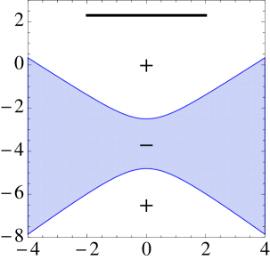
Figure 7. Signature charts for $\Re\phi(z)$ with $T=1$ in the complex $z$-plane. Left: $\mu=\mu_{c}(1)-0.1$ (subcritical). Right: $\mu=\mu_{c}(1)\approx 2.402$ (critical). The band $[a,b]$ is shown by a thick black line.

Now for $\mu$ close to $\mu_{c}(T)$ it is necessary to insert a new parametrix near $z_{c}(T)$ in terms of continuous Hermite polynomials. We will find that it is not possible to match the outer parametrix ${\bf M}_{0}^{(\text{out})}(z)$ to this local parametrix. The remedy is to introduce a pole into the outer model problem, which requires the construction of a new outer model solution.

5.1. The outer model problem for the Hermite regime

We begin by modifying the outer model problem by inserting a pole near $z_{c}(T)$. The order $k$ of this pole, which depends on $\mu$, is given in (1.19). Instead of placing the pole exactly at $z_{c}(T)$, it will be convenient to use the point $\widetilde{z}_{c}(\mu,T)$, as defined in (1.34). Note that $\widetilde{z}_{c}\to z_{c}$ as $\mu\to\mu_{c}$. The new outer model problem is the following.

Riemann–Hilbert Problem 5.1 (The Hermite regime outer model problem).

Fix $k\in\mathbb{N}$ and determine a $2\times 2$ matrix-valued function ${\bf M}_{k}^{(\rm{out})}(z)$ satisfying:

• Analyticity: ${\bf M}_{k}^{(\rm{out})}(z)$ is meromorphic in $z$ off $[a,b]$ and is Hölder continuous up to $(a,b)$ with at worst quarter-root singularities at $a$ and $b$. The only pole of ${\bf M}_{k}^{(\rm{out})}(z)$ is at $\widetilde{z}_{c}$, and ${\bf M}_{k}^{(\rm{out})}(z)(z-\widetilde{z}_{c})^{-k\sigma_{3}}$ is analytic at $z=\widetilde{z}_{c}$.

• Normalization:

  (5.4) $$\lim_{z\to\infty}{\bf M}_{k}^{(\rm{out})}(z)=\mathbb{I}.$$

• Jump condition: Orienting $[a,b]$ left-to-right, the solution satisfies (4.2).

To solve this problem we follow [7, 13] and use the functions $D(z;\mu,T)$, $R(z;\mu,T)$, and $\alpha(z;\mu,T)$ defined in (1.32), (1.33), and (1.36), respectively, as well as the constant $\alpha_{\infty}$ defined in (1.35). Note that $D_{+}(z)D_{-}(z)=-1$ for $z\in[a,b]$. We will use the following properties of $\alpha(z)$, which are shown by direct calculation.

Lemma 5.2.

$\alpha(z)$ satisfies the following.

• $\alpha(z)$ is analytic for $z\in\mathbb{C}\backslash[a,b]$.

• $\alpha_{+}(z)\alpha_{-}(z)=1$ for $z\in(a,b)$ oriented left-to-right.

• $\displaystyle\alpha(z)=-\frac{T^{3/2}}{4\pi^{2}}(z-\widetilde{z}_{c})+\mathcal{O}((z-\widetilde{z}_{c})^{2})$ for $z\in\mathbb{D}_{\widetilde{z}_{c}}$.

• $\alpha(z)$ is bounded in a full neighborhood of $[a,b]$.

• $\displaystyle\alpha(z)=\alpha_{\infty}\left(1+\frac{2\pi i}{Tz}+\mathcal{O}\left(\frac{1}{z^{2}}\right)\right)$ as $z\to\infty$.

Now the solution to the outer model problem is

(5.5) $${\bf M}_{k}^{(\rm{out})}(z):=\alpha_{\infty}^{-k\sigma_{3}}{\bf M}_{0}^{(\rm{out})}(z)\alpha(z)^{k\sigma_{3}}.$$

5.2. The local Hermite parametrix

We start by expanding $\phi(z)$ about $\widetilde{z}_{c}$:

(5.6) $$\phi(z)=-i\pi+2\pi(\mu-\mu_{c})-\frac{T}{2\pi}\sqrt{\pi^{2}-T}(z-\widetilde{z}_{c})^{2}+\mathcal{O}\left((z-\widetilde{z}_{c})^{3}\right).$$

There are a couple of salient features to observe about this expansion. First, the term $\mu-\mu_{c}$ in the order-zero coefficient is zero at criticality and grows as $\mu$ increases. This term measures the distance into the transition region, and its magnitude will determine the power of the pole needed in the outer model problem. For convenience we write

(5.7) $$\mathfrak{c}(\mu,T):=2\pi(\mu-\mu_{c}(T)).$$

Second, the order-one term is identically zero, while the order-two term is nonzero (as long as $T<\pi^{2}$, as assumed). Together, these facts dictate that the local parametrix is built out of Hermite polynomials. In a neighborhood of $\widetilde{z}_{c}$, we define the conformal map $W(z;\mu,T)$ by the identity

(5.8) $$\phi(z)=-i\pi+\mathfrak{c}-W(z)^{2}$$

and the condition that $W$ is real and increasing along $\mathbb{R}-i\delta$, with $\phi$ as defined in (3.32). The function $W$ is analytic and one-to-one for $z$ sufficiently close to $\widetilde{z}_{c}$ since $\phi(z)+i\pi-\mathfrak{c}$ vanishes to second order at $\widetilde{z}_{c}$. Define $\mathbb{D}_{\widetilde{z}_{c}}$ to be an $n$-independent disk centered at $\widetilde{z}_{c}$. The radius of the disk is chosen to be less than $\delta$ (so the disk is entirely in the lower half-plane) and is sufficiently small so that $W(z)$ is analytic and one-to-one in the disk. From (5.6) and (5.8) we see

(5.9) $$W(z)=\sqrt{\frac{T}{2\pi}}\sqrt[4]{\pi^{2}-T}(z-\widetilde{z}_{c})+\mathcal{O}\left((z-\widetilde{z}_{c})^{2}\right)$$

in its domain of definition. We seek a parametrix ${\bf M}_{k}^{(\widetilde{z}_{c})}(z)$ satisfying the following local Riemann–Hilbert problem.

Riemann–Hilbert Problem 5.3 (The Hermite regime inner model problem in $\mathbb{D}_{\widetilde{z}_{c}}$).

Fix $k\in\mathbb{N}$. Determine a $2\times 2$ matrix-valued function ${\bf M}_{k}^{(\widetilde{z}_{c})}(z)$ defined for $z\in\mathbb{D}_{\widetilde{z}_{c}}$ satisfying:

• Analyticity: ${\bf M}_{k}^{(\widetilde{z}_{c})}(z)$ is analytic for $z\in\mathbb{D}_{\widetilde{z}_{c}}$ off the contour $\mathbb{R}-i\delta$ with Hölder-continuous boundary values on the contour.

• Normalization:

  (5.10) $${\bf M}_{k}^{(\widetilde{z}_{c})}(z)=(\mathbb{I}+\mathcal{O}(n^{-1})){\bf M}_{k}^{(\rm{out})}(z)\text{ as }n\to\infty\text{ for }z\in\partial\mathbb{D}_{\widetilde{z}_{c}}.$$

• Jump condition: Orienting the jump contour left-to-right, the solution satisfies

  (5.11) $${\bf M}_{k+}^{(\widetilde{z}_{c})}(z)={\bf M}_{k-}^{(\widetilde{z}_{c})}(z)\begin{bmatrix}1&e^{2\pi i\tau-i\pi n+n\mathfrak{c}-nW(z)^{2}}\\ 0&1\end{bmatrix},\quad z\in(\mathbb{R}-i\delta)\cap\mathbb{D}_{\widetilde{z}_{c}}.$$

This problem is similar to the well-known Fokas–Its–Kitaev Riemann–Hilbert problem for (continuous) Hermite orthogonal polynomials [25]. Recall the Hermite polynomials $\mathfrak{h}_{n}(\zeta)$ and their leading coefficients $\kappa_{k}$ defined in (1.37) and (1.38), respectively. Then define the matrix-valued function

(5.12) $${\bf H}_{k}(\zeta):=\begin{cases}\begin{bmatrix}1&\mathcal{C}(e^{-\zeta^{2}})\\ 0&1\end{bmatrix},\quad k=0,\vspace{.05in}\\ \begin{bmatrix}\frac{1}{\kappa_{k}}\mathfrak{h}_{k}(\zeta)&\frac{1}{\kappa_{k}}\mathcal{C}(\mathfrak{h}_{k}(\zeta)e^{-\zeta^{2}})\\ -2\pi i\kappa_{k-1}\mathfrak{h}_{k-1}(\zeta)&-2\pi i\kappa_{k-1}\mathcal{C}(\mathfrak{h}_{k-1}(\zeta)e^{-\zeta^{2}})\end{bmatrix},&k\geq 1,\end{cases}$$

where $\mathcal{C}$ is the continuous Cauchy transform

(5.13) $$\mathcal{C}(f(\zeta)):=\frac{1}{2\pi i}\int_{\mathbb{R}}\frac{f(s)ds}{s-\zeta}.$$

It is a now-classical fact that ${\bf H}_{k}(\zeta)$ is the unique solution to the following Riemann–Hilbert problem.

Riemann–Hilbert Problem 5.4 (The Fokas–Its–Kitaev problem for Hermite polynomials).

Fix $k\in\mathbb{N}$. Determine a $2\times 2$ matrix-valued function ${\bf H}_{k}(\zeta)$ such that:

• Analyticity: ${\bf H}_{k}(\zeta)$ is analytic for $\mathbb{C}\backslash\mathbb{R}$, with Hölder-continuous boundary values from the upper and lower half-planes.

• Normalization:

  (5.14) $${\bf H}_{k}(\zeta)\zeta^{-k\sigma_{3}}=\mathbb{I}+\mathcal{O}\left(\frac{1}{\zeta}\right)\text{ as }\zeta\to\infty.$$

• Jump condition: Orienting $\mathbb{R}$ left-to-right, the solution satisfies

  (5.15) $${\bf H}_{k+}(\zeta)={\bf H}_{k-}(\zeta)\begin{bmatrix}1&e^{-\zeta^{2}}\\ 0&1\end{bmatrix},\quad\zeta\in\mathbb{R}.$$

From the large-$\zeta$ expansion of (5.12), we can improve the normalization condition (5.14) to

(5.16) $${\bf H}_{k}(\zeta)\zeta^{-k\sigma_{3}}=\mathbb{I}+\begin{bmatrix}0&\frac{-1}{2\pi i\kappa_{k}^{2}}\\ -2\pi i\kappa_{k-1}^{2}&0\end{bmatrix}\frac{1}{\zeta}+\begin{bmatrix}\frac{k^{2}-k}{4}&0\\ 0&-\frac{k^{2}+k}{4}\end{bmatrix}\frac{1}{\zeta^{2}}+\mathcal{O}\left(\frac{1}{\zeta^{3}}\right)\text{ as }\zeta\to\infty$$

(here $\kappa_{-1}:=0$). Before writing down the solution to the inner model problem we need to pull out a holomorphic prefactor from ${\bf M}_{k}^{(\text{out})}(z)$:

(5.17) $${\bf F}_{k}^{(\text{out})}(z):={\bf M}_{k}^{(\text{out})}(z)W(z)^{-k\sigma_{3}},\quad z\in\mathbb{D}_{\widetilde{z}_{c}}.$$

This function is analytic in its domain of definition from (5.9) and the analyticity condition in Riemann–Hilbert Problem 5.1. We can now solve Riemann–Hilbert Problem 5.3:

(5.18) $${\bf M}_{k}^{(\widetilde{z}_{c})}(z)={\bf F}_{k}^{(\text{out})}(z)n^{-k\sigma_{3}/2}e^{i\pi\tau\sigma_{3}}e^{n(\mathfrak{c}-i\pi)\sigma_{3}/2}{\bf H}_{k}(n^{1/2}W(z))e^{n(i\pi-\mathfrak{c})\sigma_{3}/2}e^{-i\pi\tau\sigma_{3}}.$$

5.3. The global model and error problems in the Hermite regime

We also note that there is an Airy parametrix ${\bf M}_{k}^{(a)}(z)$ defined for $z\in\mathbb{D}_{a}$ satisfying Riemann–Hilbert Problem 4.2 with the subscript 0 replaced with the subscript $k$ (and an analogous parametrix ${\bf M}_{k}^{(b)}(z)$ defined for $z\in\mathbb{D}_{b}$). In particular, the parametrices satisfy

(5.19) $${\bf M}_{k}^{(\#)}(z)={\bf M}_{k}^{(\rm{out})}(z)(\mathbb{I}+\mathcal{O}(n^{-1})),\quad z\in\partial\mathbb{D}_{\#}\quad(\#\in\{a,b\}).$$

We refer to [13] for discussion of a similar construction, as well as [18, 9, 12] for more details. We now set the global model solution to be

(5.20) $${\bf M}^{(k)}(z):=\begin{cases}{\bf M}_{k}^{\text{(out)}}(z),&z\in\mathbb{C}\backslash(\mathbb{D}_{a}\cup\mathbb{D}_{b}\cup\mathbb{D}_{\widetilde{z}_{c}}),\\ {\bf M}_{k}^{(a)}(z),&z\in\mathbb{D}_{a},\\ {\bf M}_{k}^{(b)}(z),&z\in\mathbb{D}_{b},\\ {\bf M}_{k}^{(\widetilde{z}_{c})}(z),&z\in\mathbb{D}_{\widetilde{z}_{c}}.\end{cases}$$

The error function is

(5.21) $${\bf X}_{n}^{(k)}(z):={\bf S}_{n}(z){\bf M}^{(k)}(z)^{-1}.$$

This function has jumps on the contours $\Sigma_{\text{Herm}}^{({\bf X})}$ as shown in Figure 8.

Figure 8. The jump contours $\Sigma_{\text{Herm}}^{({\bf X})}$ along with their orientations.

We write the jump conditions as

(5.22) $${\bf X}_{n+}^{(k)}(z)={\bf X}_{n-}^{(k)}(z){\bf V}_{\text{Herm}}^{({\bf X})}(z),\quad z\in\Sigma_{\text{Herm}}^{({\bf X})}.$$

The jumps are exponentially small (as $n\to\infty$) except on the three disk boundaries. Special attention should be paid to the jump on $\mathbb{R}-i\delta$ inside $\mathbb{D}_{\widetilde{z}_{c}}$, on which

(5.23) $$\begin{split}{\bf V}_{\text{Herm}}^{({\bf X})}(z)&={\bf X}_{n-}^{(k)}(z)^{-1}{\bf X}_{n+}^{(k)}(z)\\ &={\bf M}_{-}^{(k)}(z){\bf S}_{n-}(z)^{-1}{\bf S}_{n+}(z){\bf M}_{+}^{(k)}(z)^{-1}\\ &={\bf M}_{-}^{(k)}(z){\bf V}^{({\bf S})}(z){\bf V}^{({\bf M})}(z)^{-1}{\bf M}_{-}^{(k)}(z)^{-1}\\ &={\bf M}_{-}^{(k)}(z)\begin{bmatrix}1&\left(\frac{1}{1-e^{-2\pi i(nz-\tau)}}-1\right)e^{n\phi+2\pi i\tau}\\ 0&1\end{bmatrix}{\bf M}_{-}^{(k)}(z)^{-1},\quad z\in(\mathbb{R}-i\delta)\cap\mathbb{D}_{\widetilde{z}_{c}}.\end{split}$$

The function ${\bf M}^{(k)}(z)={\bf M}_{k}^{(\widetilde{z}_{c})}(z)$ is bounded, and the term in parentheses in the (12)-entry of the middle matrix in the last line of (5.23) is exponentially small. Thus the jump on this segment is exponentially close to the identity as long as $e^{n\phi}$ is not exponentially growing (or growing at a slower exponential rate than the term in parentheses). The jumps on $\partial\mathbb{D}_{a}$ and $\partial\mathbb{D}_{b}$ are $\mathcal{O}(n^{-1})$ by (5.19). Thus

(5.24) $${\bf V}_{\text{Herm}}^{({\bf X})}(z)=\mathcal{O}\left(\frac{1}{n}\right),\quad z\in\Sigma_{\text{Herm}}^{({\bf X})}\backslash\mathbb{D}_{i\mu}.$$

However, the jump on $\partial\mathbb{D}_{\widetilde{z}_{c}}$ is actually not small for certain values of $\mu$. We will address this problem in the next section by introducing a parametrix for the error. See [11, 13, 15] for similar constructions.

5.4. Parametrix for the error

We begin by gauging the size of the error jump on $\partial\mathbb{D}_{\widetilde{z}_{c}}$. Apply (5.22), (5.21), and the fact that ${\bf S}_{n}$ is continuous across $\partial\mathbb{D}_{\widetilde{z}_{c}}$ to see

(5.25) $$\left.{\bf V}_{\text{Herm}}^{({\bf X})}(z)\right|_{\partial\mathbb{D}_{\widetilde{z}_{c}}}={\bf M}_{k}^{(\widetilde{z}_{c})}(z){\bf M}_{k}^{\text{(out)}}(z)^{-1}.$$

This is calculated using (5.17), (5.18), and (5.16):

(5.26) $$\begin{split}&\left.{\bf V}_{\text{Herm}}^{({\bf X})}(z)\right|_{\partial\mathbb{D}_{\widetilde{z}_{c}}}\\ &={\bf F}_{k}^{(\text{out})}(z)n^{-k\sigma_{3}/2}e^{i\pi\tau\sigma_{3}}e^{n(\mathfrak{c}-i\pi)\sigma_{3}/2}{\bf H}_{k}(n^{1/2}W(z))W(z)^{-k\sigma_{3}}e^{n(i\pi-\mathfrak{c})\sigma_{3}/2}e^{-i\pi\tau\sigma_{3}}{\bf F}_{k}^{(\text{out})}(z)^{-1}\\ &={\bf F}_{k}^{(\text{out})}(z)n^{-k\sigma_{3}/2}e^{i\pi\tau\sigma_{3}}e^{n(\mathfrak{c}-i\pi)\sigma_{3}/2}\\ &\hskip 14.45377pt\times\left(\mathbb{I}+\frac{1}{n^{1/2}W(z)}\begin{bmatrix}0&\frac{-1}{2\pi i\kappa_{k}^{2}}\\ -2\pi i\kappa_{k-1}^{2}&0\end{bmatrix}+\frac{1}{nW(z)^{2}}\begin{bmatrix}\frac{k^{2}-k}{4}&0\\ 0&-\frac{k^{2}+k}{4}\end{bmatrix}+\mathcal{O}\left(\frac{1}{n^{3/2}}\right)\right)\\ &\hskip 14.45377pt\times e^{n(i\pi-\mathfrak{c})\sigma_{3}/2}e^{-i\pi\tau\sigma_{3}}n^{k\sigma_{3}/2}{\bf F}_{k}^{(\text{out})}(z)^{-1}.\end{split}$$

In the last equality we used that $W(z)$ is independent of $n$. Since the same is true for ${\bf F}_{k}^{(\text{out})}(z)$, we have

(5.27) $$\left.{\bf V}_{\text{Herm}}^{({\bf X})}(z)\right|_{\partial\mathbb{D}_{\widetilde{z}_{c}}}=\mathbb{I}+\begin{bmatrix}0&\mathcal{O}\left(\frac{e^{n\mathfrak{c}}}{n^{k+(1/2)}}\right)\\ \mathcal{O}\left(\frac{n^{k-(1/2)}}{e^{n\mathfrak{c}}}\right)&0\end{bmatrix}+\mathcal{O}\left(\frac{1}{n}\right)+\mathcal{O}\left(\frac{e^{n\mathfrak{c}}}{n^{k+(3/2)}}\right)+\mathcal{O}\left(\frac{n^{k-(3/2)}}{e^{n\mathfrak{c}}}\right)$$

if $k\geq 1$, and

(5.28) $$\left.{\bf V}_{\text{Herm}}^{({\bf X})}(z)\right|_{\partial\mathbb{D}_{\widetilde{z}_{c}}}=\mathbb{I}+\begin{bmatrix}0&\mathcal{O}\left(\frac{e^{n\mathfrak{c}}}{n^{k+(1/2)}}\right)\\ 0&0\end{bmatrix}+\mathcal{O}\left(\frac{e^{n\mathfrak{c}}}{n^{k+(3/2)}}\right)+\mathcal{O}\left(\frac{n^{k-(3/2)}}{e^{n\mathfrak{c}}}\right)$$

if $k=0$ (since $\kappa_{-1}\equiv 0$). For these jumps to be close to the identity, we need

(5.29) $$\left(k-\frac{1}{2}\right)\frac{\log n}{n}<\mathfrak{c}<\left(k+\frac{1}{2}\right)\frac{\log n}{n}\hskip 7.22743pt(k\geq 0).$$

Note that if $\mathfrak{c}<-\frac{1}{2n}\log n$ then the analysis in the subcritical region goes through without change. Along with (5.7), we now see that for given $n$ and $\mu$ the correct choice of $k$ is the integer such that (1.19) holds. However, if $(\mu-\mu_{c})2\pi n/\log n$ is exactly a positive half-integer, then it is not possible to choose $k$ so the jump is small on this circle. Define

(5.30) $$Q_{+}\equiv Q_{+}(T,\mu,\tau,n):=\frac{e^{2i\pi\tau}}{2\pi i\kappa_{k}^{2}}\frac{(-1)^{n}e^{n\mathfrak{c}}}{n^{k+(1/2)}},\quad Q_{-}\equiv Q_{-}(T,\mu,\tau,n):=\frac{2\pi i\kappa_{k-1}^{2}}{e^{2i\pi\tau}}\frac{n^{k-(1/2)}}{(-1)^{n}e^{n\mathfrak{c}}}.$$

We have

(5.31) $$\left.{\bf V}_{\text{Herm}}^{({\bf X})}(z)\right|_{\partial\mathbb{D}_{\widetilde{z}_{c}}}=\mathbb{I}-\frac{1}{W(z)}{\bf F}_{k}^{(\rm{out})}(z)\begin{bmatrix}0&Q_{+}\\ Q_{-}&0\end{bmatrix}{\bf F}_{k}^{(\rm{out})}(z)^{-1}+\mathcal{O}\left(\frac{1}{n}\right).$$

Note that

(5.32) $$\begin{split}Q_{+}&=\mathcal{O}(n^{-1/2}),\quad\mathfrak{c}\leq k\frac{\log n}{n},\\ Q_{-}&=\mathcal{O}(n^{-1/2}),\quad k\frac{\log n}{n}\leq\mathfrak{c}.\end{split}$$

Disregarding all terms of $\mathcal{O}(n^{-1/2})$ or smaller, we arrive at the following approximate Riemann–Hilbert problem.

Riemann–Hilbert Problem 5.5 (The parametrix for the error).

Determine the $2\times 2$ matrix-valued function ${\bf Y}_{n}^{(k)}(z)$ satisfying:

• Analyticity: ${\bf Y}_{n}^{(k)}(z)$ is analytic for $z\in\mathbb{C}\backslash\partial\mathbb{D}_{\widetilde{z}_{c}}$ with Hölder-continuous boundary values on $\partial\mathbb{D}_{\widetilde{z}_{c}}$.

• Normalization:

  (5.33) $${\bf Y}_{n}^{(k)}(z)=\mathbb{I}+\mathcal{O}\left(\frac{1}{z}\right)\text{ as }z\to\infty.$$

• Jump condition: Orienting the jump contour negatively, the solution satisfies

  (5.34) $${\bf Y}_{n+}^{(k)}(z)={\bf Y}_{n-}^{(k)}(z){\bf V}_{\rm Herm}^{({\bf Y})}(z)\equiv{\bf Y}_{n-}^{(k)}(z)\left(\mathbb{I}-\frac{1}{W(z)}{\bf F}_{k}^{(\rm{out})}(z){\bf Q}{\bf F}_{k}^{(\rm{out})}(z)^{-1}\right),\quad z\in\partial\mathbb{D}_{\widetilde{z}_{c}},$$

  where

  (5.35) $${\bf Q}:=\begin{cases}\begin{bmatrix}0&0\\ Q_{-}&0\end{bmatrix},&\displaystyle\left(k-\frac{1}{2}\right)\frac{\log n}{n}<\mathfrak{c}\leq k\frac{\log n}{n},\vspace{.05in}\\ \begin{bmatrix}0&Q_{+}\\ 0&0\end{bmatrix},&\displaystyle k\frac{\log n}{n}<\mathfrak{c}\leq\left(k+\frac{1}{2}\right)\frac{\log n}{n}.\end{cases}$$

The advantage of the function ${\bf Y}_{n}^{(k)}(z)$ is that the ratio

(5.36) $${\bf Z}_{n}^{(k)}(z):={\bf X}_{n}^{(k)}(z){\bf Y}_{n}^{(k)}(z)^{-1}$$

satisfies the jump condition

(5.37) $${\bf Z}_{n+}^{(k)}(z)={\bf Z}_{n-}^{(k)}(z){\bf V}_{\text{Herm}}^{({\bf Z})}(z),\quad z\in\Sigma_{\text{Herm}}^{({\bf Z})}\equiv\Sigma_{\text{Herm}}^{({\bf X})},$$

where ${\bf V}_{\text{Herm}}^{({\bf Z})}(z)$ is uniformly $o(1)$ as $n\to\infty$ (in the Hermite regime). The jump $\Sigma_{\text{Herm}}^{({\bf Z})}$ is clearly controlled for $z\in\Sigma_{\text{Herm}}^{({\bf Z})}\backslash\partial\mathbb{D}_{\widetilde{z}_{c}}$ (since ${\bf V}_{\text{Herm}}^{({\bf X})}(z)$ is controlled and ${\bf Y}_{n}^{(k)}(z)$ has no jump here). On the other hand, we also have

(5.38) $$\begin{split}\left.{\bf V}_{\text{Herm}}^{({\bf Z})}(z)\right|_{\partial\mathbb{D}_{\widetilde{z}_{c}}}&={\bf Z}_{n-}^{(k)}(z)^{-1}{\bf Z}_{n+}^{(k)}(z)\\ &={\bf Y}_{n-}^{(k)}(z){\bf X}_{n-}^{(k)}(z)^{-1}{\bf X}_{n+}(z){\bf Y}_{n+}^{(k)}(z)^{-1}\\ &={\bf Y}_{n-}^{(k)}(z){\bf V}_{\text{Herm}}^{({\bf X})}(z){\bf V}_{\text{Herm}}^{({\bf Y})}(z)^{-1}{\bf Y}_{n-}^{(k)}(z)^{-1}.\end{split}$$

Thus, recalling (5.31) and (5.34), for $z\in\mathbb{D}_{\widetilde{z}_{c}}$,

(5.39) $${\bf V}_{\text{Herm}}^{({\bf Z})}(z)=\mathbb{I}-\frac{1}{W(z)}{\bf Y}_{n-}^{(k)}(z){\bf F}_{k}^{(\text{out})}(z)\widehat{\bf Q}{\bf F}_{k}^{(\text{out})}(z)^{-1}{\bf Y}_{n-}^{(k)}(z)^{-1}+\mathcal{O}\left(\frac{1}{n}\right),$$

where we have defined

(5.40) $$\widehat{\bf Q}:=\begin{cases}\begin{bmatrix}0&Q_{+}\\ 0&0\end{bmatrix},&\displaystyle\left(k-\frac{1}{2}\right)\frac{\log n}{n}<\mathfrak{c}\leq k\frac{\log n}{n},\vspace{.05in}\\ \begin{bmatrix}0&0\\ Q_{-}&0\end{bmatrix},&\displaystyle k\frac{\log n}{n}<\mathfrak{c}\leq\left(k+\frac{1}{2}\right)\frac{\log n}{n}.\end{cases}$$

From (5.32) we see $\widehat{\bf Q}=\mathcal{O}(n^{-1/2})$, and thus

(5.41) $${\bf V}_{\text{Herm}}^{({\bf Z})}(z)=\mathcal{O}(n^{-1/2})\quad\text{for all }z\in\Sigma^{({\bf Z})}.$$

We now solve Riemann–Hilbert Problem 5.5 exactly following [13], §3.5.2. The function

(5.42) $${\bf\widetilde{Y}}_{n}^{(k)}(z):=\begin{cases}{\bf Y}_{n}^{(k)}(z),&z\in\mathbb{C}\backslash\mathbb{D}_{\widetilde{z}_{c}},\\ \displaystyle{\bf Y}_{n}^{(k)}(z)\left(\mathbb{I}-\frac{1}{W(z)}{\bf F}_{k}^{(\rm{out})}(z){\bf Q}{\bf F}_{k}^{(\rm{out})}(z)^{-1}\right),&z\in\mathbb{D}_{\widetilde{z}_{c}}\end{cases}$$

is the (meromorphic) continuation of ${\bf Y}_{n}^{(k)}(z)$ from the exterior to the interior of $\mathbb{D}_{\widetilde{z}_{c}}$. This function is meromorphic in the entire complex $z$-plane with exactly one simple pole at $\widetilde{z}_{c}$. Furthermore, $\lim_{z\to\infty}{\bf Y}_{n}^{(k)}(z)=\mathbb{I}$, so we can write

(5.43) $${\bf\widetilde{Y}}_{n}^{(k)}(z)=\mathbb{I}+\frac{1}{z-\widetilde{z}_{c}}{\bf B},$$

where ${\bf B}$ is independent of $z$. Our next goal is to determine the $2\times 2$ matrix ${\bf B}\equiv{\bf B}(T,\mu,\tau,n)$. Since ${\bf Y}_{n}^{(k)}(z)$ is analytic at $z=\widetilde{z}_{c}$, we have

(5.44) $${\bf Y}_{n}^{(k)}(z)=\left(\mathbb{I}+\frac{1}{z-\widetilde{z}_{c}}{\bf B}\right)\left(\mathbb{I}+\frac{1}{W(z)}{\bf F}_{k}^{(\rm{out})}(z){\bf Q}{\bf F}_{k}^{(\rm{out})}(z)^{-1}\right)=\mathcal{O}(1)\text{ for }z\to\widetilde{z}_{c}.$$

We expand the middle quantity at $z=\widetilde{z}_{c}$. Write

(5.45) $${\bf F}_{k}^{(\text{out})}(z)={\bf F}_{0}+{\bf F}_{1}(z-\widetilde{z}_{c})+\mathcal{O}\left((z-\widetilde{z}_{c})^{2}\right)$$

and

(5.46) $$\begin{split}&W(z)=(z-\widetilde{z}_{c})W_{1}+(z-\widetilde{z}_{c})^{2}W_{2}+\mathcal{O}\left((z-\widetilde{z}_{c})^{3}\right)\\ &\Rightarrow\frac{1}{W(z)}=\frac{1}{(z-\widetilde{z}_{c})W_{1}}-\frac{W_{2}}{W_{1}^{2}}+\mathcal{O}(z-\widetilde{z}_{c}),\end{split}$$

where ${\bf F}_{0}$, ${\bf F}_{1}$, $W_{1}$, and $W_{2}$ are independent of $z$. Note that

(5.47) $$W_{1}=\sqrt{\frac{T}{2\pi}}\sqrt[4]{\pi^{2}-T}$$

from (5.9). Then we must have

(5.48) $$\frac{{\bf B}{\bf F}_{0}{\bf Q}{\bf F}_{0}^{-1}}{(z-\widetilde{z}_{c})^{2}W_{1}}+\frac{1}{z-\widetilde{z}_{c}}\left({\bf B}+\frac{{\bf F}_{0}{\bf Q}{\bf F}_{0}^{-1}}{W_{1}}+\frac{{\bf B}{\bf F}_{1}{\bf Q}{\bf F}_{0}^{-1}}{W_{1}}-\frac{{\bf B}{\bf F}_{0}{\bf Q}{\bf F}_{0}^{-1}{\bf F}_{1}{\bf F}_{0}^{-1}}{W_{1}}-\frac{W_{2}{\bf B}{\bf F}_{0}{\bf Q}{\bf F}_{0}^{-1}}{W_{1}^{2}}\right)={\bf 0}.$$

Separating powers of $z-\widetilde{z}_{c}$ (and using the invertibility of ${\bf F}_{0}$, which can be checked via explicit computation) gives the system of equations

(5.49) $${\bf B}{\bf F}_{0}{\bf Q}={\bf 0},\quad{\bf B}{\bf F}_{0}+\frac{1}{W_{1}}{\bf F}_{0}{\bf Q}+\frac{1}{W_{1}}{\bf B}{\bf F}_{1}{\bf Q}={\bf 0}.$$

The first equation shows that the first column of ${\bf B}{\bf F}_{0}$ is zero when ${\bf Q}$ is strictly upper triangular, and the second column of ${\bf B}{\bf F}_{0}$ is zero when ${\bf Q}$ is strictly lower triangular. Solving the second equation then gives

(5.50) $${\bf B}=\begin{cases}\displaystyle\frac{-{\bf F}_{0}{\bf Q}{\bf F}_{0}^{-1}}{W_{1}+[{\bf F}_{0}^{-1}{\bf F}_{1}]_{12}Q_{-}},&\displaystyle\left(k-\frac{1}{2}\right)\frac{\log n}{n}<\mathfrak{c}\leq k\frac{\log n}{n},\vspace{.05in}\\ \displaystyle\frac{-{\bf F}_{0}{\bf Q}{\bf F}_{0}^{-1}}{W_{1}+[{\bf F}_{0}^{-1}{\bf F}_{1}]_{21}Q_{+}},&\displaystyle k\frac{\log n}{n}<\mathfrak{c}\leq\left(k+\frac{1}{2}\right)\frac{\log n}{n}.\end{cases}$$

We will need the (11)-entry of ${\bf B}$. Start with

(5.51) $$[{\bf B}]_{11}=\begin{cases}\displaystyle\frac{-\frac{Q_{-}}{W_{1}}[{\bf F}_{0}]_{12}[{\bf F}_{0}]_{22}}{1+\frac{Q_{-}}{W_{1}}[{\bf F}_{0}^{-1}{\bf F}_{1}]_{12}},&\displaystyle\left(k-\frac{1}{2}\right)\frac{\log n}{n}<\mathfrak{c}\leq k\frac{\log n}{n},\vspace{.05in}\\ \displaystyle\frac{\frac{Q_{+}}{W_{1}}[{\bf F}_{0}]_{11}[{\bf F}_{0}]_{21}}{1+\frac{Q_{+}}{W_{1}}[{\bf F}_{0}^{-1}{\bf F}_{1}]_{21}},&\displaystyle k\frac{\log n}{n}<\mathfrak{c}\leq\left(k+\frac{1}{2}\right)\frac{\log n}{n}.\end{cases}$$

Observe that ${\bf F}_{0}\equiv{\bf F}_{k}^{(\text{out})}(\widetilde{z}_{c})$. We introduce the notations

(5.52) $$\gamma_{*}\equiv\gamma_{*}(T):=\gamma(\widetilde{z}_{c})=\frac{1}{\sqrt{\pi}}\left(\sqrt{\pi^{2}-T}+i\sqrt{T}\right)^{1/2}$$

(here the square root is the principal branch) and

(5.53) $$\frac{\alpha_{*}}{W_{*}}:=\lim_{z\to\widetilde{z}_{c}}\frac{\alpha(z)}{W(z)}=\frac{-T}{(2\pi)^{3/2}\sqrt[4]{\pi^{2}-T}},$$

obtained via the local expansions near $z=\widetilde{z}_{c}$ in Lemma 5.2(c) for $\alpha(z)$ and Equation (5.9) for $W(z)$. Then from (5.17), (5.5), and (4.3) we have

(5.54) $${\bf F}_{0}=\alpha_{\infty}^{-k\sigma_{3}}\begin{bmatrix}\displaystyle\frac{\gamma_{*}+\gamma_{*}^{-1}}{2}&\displaystyle\frac{\gamma_{*}-\gamma_{*}^{-1}}{-2i}\\ \displaystyle\frac{\gamma_{*}-\gamma_{*}^{-1}}{2i}&\displaystyle\frac{\gamma_{*}+\gamma_{*}^{-1}}{2}\end{bmatrix}\left(\frac{\alpha_{*}}{W_{*}}\right)^{k\sigma_{3}}.$$

Together, the previous three equations yield

(5.55) $$\begin{split}[{\bf F}_{0}]_{11}[{\bf F}_{0}]_{21}&=-\frac{i}{4}(\gamma_{*}^{2}-\gamma_{*}^{-2})\left(\frac{\alpha_{*}}{W_{*}}\right)^{2k}=\frac{T^{(4k+1)/2}}{(2\pi)^{3k+1}(\pi^{2}-T)^{k/2}},\\ [{\bf F}_{0}]_{12}[{\bf F}_{0}]_{22}&=\frac{i}{4}(\gamma_{*}^{2}-\gamma_{*}^{-2})\left(\frac{\alpha_{*}}{W_{*}}\right)^{-2k}=-\frac{(2\pi)^{3k-1}(\pi^{2}-T)^{k/2}}{T^{(4k-1)/2}}.\end{split}$$

At this point we define the quantities

(5.56) $$\begin{split}R_{+}\equiv R_{+}(T,\mu,n)&:=\frac{iT^{2k}}{(2\pi)^{(6k+3)/2}(\pi^{2}-T)^{(2k+1)/4}\kappa_{k}^{2}}\cdot\frac{(-1)^{n+1}e^{n\mathfrak{c}}}{n^{k+(1/2)}},\\ R_{-}\equiv R_{-}(T,\mu,n)&:=\frac{(2\pi)^{(6k+1)/2}(\pi^{2}-T)^{(2k-1)/4}\kappa_{k-1}^{2}}{iT^{2k}}\cdot\frac{n^{k-(1/2)}}{(-1)^{n+1}e^{n\mathfrak{c}}},\end{split}$$

so that (using (5.30), (5.47), and (5.55))

(5.57) $$\frac{Q_{+}}{W_{1}}[{\bf F}_{0}]_{11}[{\bf F}_{0}]_{21}=R_{+}e^{2\pi i\tau},\quad-\frac{Q_{-}}{W_{1}}[{\bf F}_{0}]_{12}[{\bf F}_{0}]_{22}=R_{-}e^{-2\pi i\tau}.$$

We also have

(5.58) $$\begin{split}{\bf F}_{1}\equiv\left.\frac{d{\bf F}_{k}^{(\text{out})}(z)}{dz}\right|_{z=\widetilde{z}_{c}}=&\alpha_{\infty}^{-k\sigma_{3}}\frac{\gamma^{\hskip 1.4457pt\prime}(\widetilde{z}_{c})}{\gamma_{*}}\begin{bmatrix}\displaystyle\frac{\gamma_{*}-\gamma_{*}^{-1}}{2}&\displaystyle\frac{\gamma_{*}+\gamma_{*}^{-1}}{-2i}\\ \displaystyle\frac{\gamma_{*}+\gamma_{*}^{-1}}{2i}&\displaystyle\frac{\gamma_{*}-\gamma_{*}^{-1}}{2}\end{bmatrix}\left(\frac{\alpha_{*}}{W_{*}}\right)^{k\sigma_{3}}\\ &+\alpha_{\infty}^{-k\sigma_{3}}\begin{bmatrix}\displaystyle\frac{\gamma_{*}+\gamma_{*}^{-1}}{2}&\displaystyle\frac{\gamma_{*}-\gamma_{*}^{-1}}{-2i}\\ \displaystyle\frac{\gamma_{*}-\gamma_{*}^{-1}}{2i}&\displaystyle\frac{\gamma_{*}+\gamma_{*}^{-1}}{2}\end{bmatrix}\frac{d}{dz}\left.\left(\left(\frac{\alpha(z)}{W(z)}\right)^{k\sigma_{3}}\right)\right|_{z=\widetilde{z}_{c}}.\end{split}$$

Direct calculation shows

(5.59) $$\frac{\gamma^{\hskip 1.4457pt\prime}(\widetilde{z}_{c})}{\gamma_{*}}=\frac{T^{3/2}}{4\pi^{2}}.$$

The preceding four equations show

(5.60) $$\begin{split}[{\bf F}_{0}^{-1}{\bf F}_{1}]_{12}&=i\frac{\gamma^{\hskip 1.4457pt\prime}(\widetilde{z}_{c})}{\gamma_{*}}\left(\frac{\alpha_{*}}{W_{*}}\right)^{-2k}=\frac{(2\pi)^{3k-2}(\pi^{2}-T)^{k/2}i}{T^{(4k-3)/2}},\\ [{\bf F}_{0}^{-1}{\bf F}_{1}]_{21}&=-i\frac{\gamma^{\hskip 1.4457pt\prime}(\widetilde{z}_{c})}{\gamma_{*}}\left(\frac{\alpha_{*}}{W_{*}}\right)^{2k}=\frac{T^{(4k+3)/2}}{(2\pi)^{3k+2}(\pi^{2}-T)^{k/2}i}.\end{split}$$

Thus, from (5.30), (5.47), (5.56), and (5.60),

(5.61) $$\frac{Q_{+}}{W_{1}}[{\bf F}_{0}^{-1}{\bf F}_{1}]_{21}=\frac{TR_{+}}{2\pi i}e^{2\pi i\tau}\quad\text{and}\quad\frac{Q_{-}}{W_{1}}[{\bf F}_{0}^{-1}{\bf F}_{1}]_{12}=-\frac{TR_{-}}{2\pi i}e^{-2\pi i\tau}.$$

Therefore

(5.62) $$[{\bf B}]_{11}=\begin{cases}\displaystyle\frac{R_{-}e^{-2\pi i\tau}}{1-\frac{TR_{-}}{2\pi i}e^{-2\pi i\tau}},&\displaystyle\left(k-\frac{1}{2}\right)\frac{\log n}{n}<\mathfrak{c}\leq k\frac{\log n}{n},\vspace{.05in}\\ \displaystyle\frac{R_{+}e^{2\pi i\tau}}{1+\frac{TR_{+}}{2\pi i}e^{2\pi i\tau}},&\displaystyle k\frac{\log n}{n}<\mathfrak{c}\leq\left(k+\frac{1}{2}\right)\frac{\log n}{n}.\end{cases}$$

Later we will need that fact, that follows directly from (5.50) and (5.35), that

(5.63) $${\bf B}=\begin{cases}\mathcal{O}(Q_{-}),&\displaystyle\left(k-\frac{1}{2}\right)\frac{\log n}{n}<\mathfrak{c}\leq k\frac{\log n}{n},\vspace{.05in}\\ \mathcal{O}(Q_{+}),&\displaystyle k\frac{\log n}{n}<\mathfrak{c}\leq\left(k+\frac{1}{2}\right)\frac{\log n}{n}.\end{cases}$$

Putting together (5.42) and (5.43) shows

(5.64) $${\bf Y}_{n}^{(k)}(z):=\begin{cases}\left(\mathbb{I}+\frac{1}{z-\widetilde{z}_{c}}{\bf B}\right),&z\in\mathbb{C}\backslash\mathbb{D}_{\widetilde{z}_{c}},\\ \left(\mathbb{I}+\frac{1}{z-\widetilde{z}_{c}}{\bf B}\right)\left(\mathbb{I}+\frac{1}{W(z)}{\bf F}_{k}^{(\rm{out})}(z){\bf Q}{\bf F}_{k}^{(\rm{out})}(z)^{-1}\right),&z\in\mathbb{D}_{\widetilde{z}_{c}}.\end{cases}$$

5.5. Winding numbers in the Hermite regime

We now determine the winding numbers in the Hermite regime.

Proof of Theorem 1.2 (Hermite regime winding number asymptotics).

Recalling Lemma 3.2, to compute the winding probabilities we will first determine $[{\bf P}_{n,1}]_{11}$. Repeating the logic leading to Equation (4.9) in the subcritical case shows

(5.65) $$\mathbf{P}_{n}(z)=\begin{bmatrix}1&0\\ 0&-2\pi i\end{bmatrix}^{-1}e^{n\ell\sigma_{3}/2}\mathbf{Z}_{n}^{(k)}(z)\mathbf{Y}_{n}^{(k)}(z)\mathbf{M}^{(k)}(z)e^{n(g(z)-\ell/2)\sigma_{3}}\begin{bmatrix}1&0\\ 0&-2\pi i\end{bmatrix}$$

for $z\in\mathbb{C}\backslash\{z|-\delta\leq\Im z\leq\mu+\epsilon\}$. We have the large-$z$ expansions

(5.66) $${\bf Y}_{n}^{(k)}(z)=\mathbb{I}+\frac{\bf B}{z}+\mathcal{O}\left(\frac{1}{z^{2}}\right),\quad{\bf Z}_{n}^{(k)}(z)=\mathbb{I}+\frac{{\bf Z}_{n,1}^{(k)}}{z}+\mathcal{O}\left(\frac{1}{z^{2}}\right),$$

where the relevant entry of ${\bf Z}_{n,1}^{(k)}$ will be computed below. Therefore, using (3.19) for $g_{1}$,

(5.67) $$\begin{split}\mathbb{I}+\frac{\mathbf{P}_{n,1}}{z}+\mathcal{O}\left(\frac{1}{z^{2}}\right)=&\begin{bmatrix}1&0\\ 0&-2\pi i\end{bmatrix}^{-1}e^{n\ell\sigma_{3}/2}\left(\mathbb{I}+\frac{\mathbf{Z}_{n,1}^{(k)}+{\bf B}+{\bf M}_{1}^{(k)}}{z}+\mathcal{O}\left(\frac{1}{z^{2}}\right)\right)\\ &\times\exp\left(-n\left(\frac{i\mu}{z}+\mathcal{O}\left(\frac{1}{z^{2}}\right)\right)\sigma_{3}\right)e^{-(n\ell/2)\sigma_{3}}\begin{bmatrix}1&0\\ 0&-2\pi i\end{bmatrix}.\end{split}$$

We see

(5.68) $$[\mathbf{P}_{n,1}]_{11}=-in\mu+\left[\mathbf{Z}_{n,1}^{(k)}\right]_{11}+\left[{\bf B}\right]_{11}+\left[\mathbf{M}_{1}^{(k)}\right]_{11}.$$

We have already obtained a formula for $[{\bf B}]_{11}$ in (5.62). Our next step is to find $\left[{\bf M}_{1}^{(k)}\right]_{11}$. Now ${\bf M}^{(k)}(z)={\bf M}_{k}^{\text{(out)}}(z)$ for $z$ sufficiently large by (5.20). From (5.5), (4.3), (1.28), and Lemma 5.2(e),

(5.69) $$\left[{\bf M}_{k}^{\text{(out)}}(z)\right]_{11}=\frac{\gamma(z)+\gamma(z)^{-1}}{2}\left(\frac{\alpha(z)}{\alpha_{\infty}}\right)^{k}=\left(1+\mathcal{O}\left(\frac{1}{z^{2}}\right)\right)\left(1+\frac{2\pi ik}{Tz}+\mathcal{O}\left(\frac{1}{z^{2}}\right)\right).$$

Therefore

(5.70) $$\left[{\bf M}_{1}^{(k)}\right]_{11}=\frac{2i\pi k}{T}.$$

Now we find $\left[{\bf Z}_{n,1}^{(k)}\right]_{11}$. As we have shown ${\bf V}_{\text{Herm}}^{({\bf Z})}(z)=\mathcal{O}(n^{-1/2})$ for $z\in\partial\mathbb{D}_{\widetilde{z}_{c}}$ and is exponentially small for $z\in\Sigma_{\text{Herm}}^{({\bf Z})}\backslash\partial\mathbb{D}_{\widetilde{z}_{c}}$, it follows that ${\bf Z}_{n}(z)$ can be solved by a convergent Neumann series (see, for example, [31, §5] for a similar analysis), and in particular

(5.71) $${\bf Z}_{n,1}^{(k)}=\frac{-1}{2\pi i}\oint_{\partial\mathbb{D}_{\widetilde{z}_{c}}}\left({\bf V}_{\text{Herm}}^{({\bf Z})}(u)-\mathbb{I}\right)du+\mathcal{O}\left(\frac{1}{n}\right).$$

A residue calcuation using (5.71), (5.39), (5.45), (5.47), and the fact that $\partial\mathbb{D}_{\widetilde{z}_{c}}$ is negatively oriented gives

(5.72) $${\bf Z}_{n,1}^{(k)}=\frac{-1}{W_{1}}{\bf Y}_{n}^{(k)}(\widetilde{z}_{c}){\bf F}_{0}\widehat{\bf Q}{\bf F}_{0}^{-1}{\bf Y}_{n}^{(k)}(\widetilde{z}_{c})^{-1}+\mathcal{O}\left(\frac{1}{n}\right).$$

Equations (5.44) and (5.63) show us that

(5.73) $${\bf Y}_{n}^{(k)}(\widetilde{z}_{c})=\begin{cases}\mathbb{I}+\mathcal{O}(Q_{-}),&(k-\frac{1}{2})\frac{\log n}{n}<\mathfrak{c}<k\frac{\log n}{n},\vspace{.05in}\\ \mathbb{I}+\mathcal{O}(Q_{+}),&k\frac{\log n}{n}<\mathfrak{c}<(k+\frac{1}{2})\frac{\log n}{n}.\end{cases}$$

The definition (5.40) of $\widehat{\bf Q}$ and the fact that $Q_{+}Q_{-}=\mathcal{O}(n^{-1})$ lead to

(5.74) $${\bf Z}_{n,1}^{(k)}=\frac{-1}{W_{1}}{\bf F}_{0}\widehat{\bf Q}{\bf F}_{0}^{-1}+\mathcal{O}\left(\frac{1}{n}\right).$$

Direct calculation (using $\det{\bf F}_{0}\equiv 1$, which follows from ${\bf F}_{0}\equiv{\bf F}_{k}^{(\text{out})}(\widetilde{z}_{c})$ and $\det{\bf F}_{k}^{(\text{out})}(z)\equiv 1$) now gives

(5.75) $$\left[{\bf Z}_{n,1}^{(k)}\right]_{11}=\begin{cases}\frac{Q_{+}}{W_{1}}\left[{\bf F}_{0}\right]_{11}\left[{\bf F}_{0}\right]_{21}+\mathcal{O}\left(\frac{1}{n}\right),&(k-\frac{1}{2})\frac{\log n}{n}<\mathfrak{c}\leq k\frac{\log n}{n},\vspace{.05in}\\ -\frac{Q_{-}}{W_{1}}\left[{\bf F}_{0}\right]_{12}\left[{\bf F}_{0}\right]_{22}+\mathcal{O}\left(\frac{1}{n}\right),&k\frac{\log n}{n}<\mathfrak{c}\leq(k+\frac{1}{2})\frac{\log n}{n}.\end{cases}$$

Equation (5.57) gives

(5.76) $$\left[{\bf Z}_{n,1}^{(k)}\right]_{11}=\begin{cases}R_{+}e^{2\pi i\tau}+\mathcal{O}\left(\frac{1}{n}\right),&(k-\frac{1}{2})\frac{\log n}{n}<\mathfrak{c}\leq k\frac{\log n}{n},\vspace{.05in}\\ R_{-}e^{-2\pi i\tau}+\mathcal{O}\left(\frac{1}{n}\right),&k\frac{\log n}{n}<\mathfrak{c}\leq(k+\frac{1}{2})\frac{\log n}{n}.\end{cases}$$

This is similar to the expression (5.62) for $[{\bf B}]_{11}$. In fact, since (cf. (5.32))

(5.77) $$\begin{split}R_{+}&=\mathcal{O}(n^{-1/2}),\quad\left(k-\frac{1}{2}\right)\frac{\log n}{n}<\mathfrak{c}\leq k\frac{\log n}{n},\\ R_{-}&=\mathcal{O}(n^{-1/2}),\quad k\frac{\log n}{n}<\mathfrak{c}\leq\left(k+\frac{1}{2}\right)\frac{\log n}{n},\end{split}$$

we can add appropriate denominators with no extra error term:

(5.78) $$\left[{\bf Z}_{n,1}^{(k)}\right]_{11}=\begin{cases}\displaystyle\frac{R_{+}e^{2\pi i\tau}}{1+\frac{TR_{+}}{2\pi i}e^{2\pi i\tau}}+\mathcal{O}\left(\frac{1}{n}\right),&(k-\frac{1}{2})\frac{\log n}{n}<\mathfrak{c}\leq k\frac{\log n}{n},\vspace{.05in}\\ \displaystyle\frac{R_{-}e^{-2\pi i\tau}}{1-\frac{TR_{-}}{2\pi i}e^{-2\pi i\tau}}+\mathcal{O}\left(\frac{1}{n}\right),&k\frac{\log n}{n}<\mathfrak{c}\leq(k+\frac{1}{2})\frac{\log n}{n}.\end{cases}$$

The advantage is that now, from (5.68), (5.62), (5.70), and (5.78), $[{\bf P}_{n,1}]_{11}$ takes the simplified form

(5.79) $$[{\bf P}_{n,1}]_{11}=-in\mu+\frac{2i\pi k}{T}+\frac{R_{+}e^{2\pi i\tau}}{1+\frac{TR_{+}}{2\pi i}e^{2\pi i\tau}}+\frac{R_{-}e^{-2\pi i\tau}}{1-\frac{TR_{-}}{2\pi i}e^{-2\pi i\tau}}+\mathcal{O}\left(\frac{1}{n}\right).$$

The $\mathcal{O}(n^{-1})$ error terms are uniformly bounded in $\tau$ (and therefore integrable with respect to $\tau$). Combining Proposition 2.2, (3.8), and (5.79) shows

(5.80) $$\begin{split}\log&\left(\frac{\mathcal{H}_{n}(T,\mu,\tau)}{\mathcal{H}_{n}(T,\mu,\epsilon(n))}\right)=\int_{\epsilon(n)}^{\tau}\left(inT\mu+T[\mathbf{P}_{n,1}(T,\mu,v)]_{11}\right)\,dv\\ &\hskip 14.45377pt=\int_{\epsilon(n)}^{\tau}\left[2\pi ik+\frac{TR_{+}e^{2\pi iv}}{1+\frac{TR_{+}}{2\pi i}e^{2\pi iv}}+\frac{TR_{-}e^{-2\pi iv}}{1-\frac{TR_{-}}{2\pi i}e^{-2\pi iv}}\right]\,dv+\mathcal{O}\left(\frac{1}{n}\right)\\ &\hskip 14.45377pt=2ik\pi(\tau-\epsilon(n))+\log\left(1+\frac{TR_{+}}{2\pi i}e^{2\pi i\tau}\right)-\log\left(1+\frac{TR_{+}}{2\pi i}e^{2\pi i\epsilon(n)}\right)\\ &\hskip 32.52127pt+\log\left(1-\frac{TR_{-}}{2\pi i}e^{-2\pi i\tau}\right)-\log\left(1-\frac{TR_{-}}{2\pi i}e^{-2\pi i\epsilon(n)}\right)+\mathcal{O}\left(\frac{1}{n}\right).\end{split}$$

Exponentiating and using $R_{+}R_{-}=\mathcal{O}(n^{-1})$ from (5.56) and $e^{2\pi i\epsilon(n)}=(-1)^{n+1}$ from (1.5) gives

(5.81) $$\frac{\mathcal{H}_{n}(T,\mu,\tau)}{\mathcal{H}_{n}(T,\mu,\epsilon(n))}=\frac{(-1)^{-(n+1)k}}{1+\frac{(-1)^{n+1}T}{2\pi i}(R_{+}-R_{-})}\left(1+\frac{TR_{+}}{2\pi i}e^{2\pi i\tau}-\frac{TR_{-}}{2\pi i}e^{-2\pi i\tau}\right)e^{2ik\pi\tau}+\mathcal{O}\left(\frac{1}{n}\right).$$

We can now compute the winding numbers using (1.16):

(5.82) $$\begin{split}&\mathbb{P}(\mathcal{W}_{n}(T,\mu)=\omega)\\ &=\frac{(-1)^{(n+1)(\omega-k)}}{1+\frac{(-1)^{n+1}T}{2\pi i}(R_{+}-R_{-})}\int_{0}^{1}\left(1+\frac{TR_{+}}{2\pi i}e^{2\pi i\tau}-\frac{TR_{-}}{2\pi i}e^{-2\pi i\tau}\right)e^{2\pi i\tau(k-\omega)}d\tau+\mathcal{O}\left(\frac{1}{n}\right)\\ &=\begin{cases}\displaystyle\frac{\frac{1}{2\pi i}(-1)^{n}TR_{-}}{1+\frac{1}{2\pi i}(-1)^{n+1}TR_{+}+\frac{1}{2\pi i}(-1)^{n}TR_{-}}+\mathcal{O}\left(\frac{1}{n}\right),&\omega=k-1,\vspace{.05in}\\ \displaystyle\frac{1}{1+\frac{1}{2\pi i}(-1)^{n+1}TR_{+}+\frac{1}{2\pi i}(-1)^{n}TR_{-}}+\mathcal{O}\left(\frac{1}{n}\right),&\omega=k,\vspace{.05in}\\ \displaystyle\frac{\frac{1}{2\pi i}(-1)^{n+1}TR_{+}}{1+\frac{1}{2\pi i}(-1)^{n+1}TR_{+}+\frac{1}{2\pi i}(-1)^{n}TR_{-}}+\mathcal{O}\left(\frac{1}{n}\right),&\omega=k+1,\vspace{.1in}\\ \displaystyle\mathcal{O}\left(\frac{1}{n}\right),&\text{otherwise}.\end{cases}\end{split}$$

This can be written in the simplified form (1.20) using the formulas (5.7) and (1.38) for $\mathfrak{c}$ and $\kappa_{k}$. This completes the proof of Theorem 1.2. ∎

5.6. Orthogonal polynomial asymptotics in the Hermite regime

We now prove the results for orthogonal polynomials in the Hermite regime, starting with Theorem 1.4.

Proof of Theorem 1.4 (Orthogonal polynomials in the Hermite regime).

From (3.4), (3.12), (3.23), (3.27), (5.21), and (5.36),

(5.83) $$p_{n,n}^{(T,\mu,\tau)}(z)=[{\bf P}_{n}(z)]_{11}=[{\bf Z}_{n}^{(k)}(z){\bf Y}_{n}^{(k)}(z){\bf M}^{(k)}(z)]_{11}e^{ng(z)}$$

for $z\in\mathbb{C}\backslash(\Omega_{+}\cup\Omega_{-})$ (here we have used the fact that ${\bf D}_{+}^{u}(z)$ and ${\bf D}_{-}^{u}(z)$ are upper-triangular to obtain the result for $-\delta\leq\Im z\leq\mu$). From (5.41) and the small-norm theory of Riemann–Hilbert problems [19], we have

(5.84) $${\bf Z}_{n}^{(k)}(z)=\mathbb{I}+\mathcal{O}(n^{-1/2}).$$

Furthermore, from (5.64), (5.63), (5.35), and (5.30), we also have

(5.85) $${\bf Y}_{n}^{(k)}(z)=\mathbb{I}+\mathcal{O}\left(\frac{e^{2\pi n(\mu-\mu_{c})}}{n^{k+\frac{1}{2}}}\right)+\mathcal{O}\left(\frac{n^{k-\frac{1}{2}}}{e^{2\pi n(\mu-\mu_{c})}}\right).$$

Thus we have

(5.86) $$p_{n,n}^{(T,\mu,\tau)}(z)=e^{ng(z)}[{\bf M}^{(k)}(z)]_{11}\left(1+\mathcal{O}\left(\frac{e^{2\pi n(\mu-\mu_{c})}}{n^{k+\frac{1}{2}}}\right)+\mathcal{O}\left(\frac{n^{k-\frac{1}{2}}}{e^{2\pi n(\mu-\mu_{c})}}\right)\right).$$

By (5.20), (5.5), and (4.3),

(5.87) $$[{\bf M}^{(k)}(z)]_{11}=\left(\frac{\alpha(z)}{\alpha_{\infty}}\right)^{k}\left(\frac{\gamma(z)+\gamma(z)^{-1}}{2}\right),\quad z\in\mathbb{C}\backslash(\mathbb{D}_{a}\cup\mathbb{D}_{b}\cup\mathbb{D}_{\widetilde{z}_{c}}),$$

which establishes (1.39) and proves part (a).

For $z$ on the band but outside the Airy neighborhoods $\mathbb{D}_{a}$ and $\mathbb{D}_{b}$, we have (similar to (5.83) but taking into account the jumps on the lens boundaries)

(5.88) $$p_{n,n}^{(T,\mu,\tau)}(z)=[{\bf Z}_{n}^{(k)}(z){\bf Y}_{n}^{(k)}(z){\bf M}_{-}^{(k)}(z)]_{11}e^{ng_{-}(z)}-[{\bf Z}_{n}^{(k)}(z){\bf Y}_{n}^{(k)}(z){\bf M}_{-}^{(k)}(z)]_{12}e^{ng_{+}(z)}.$$

From (5.84) and (5.85),

(5.89) $$\begin{split}&p_{n,n}^{(T,\mu,\tau)}(z)\\ &=\left([{\bf M}_{-}^{(k)}(z)]_{11}e^{ng_{-}(z)}-[{\bf M}_{-}^{(k)}(z)]_{12}e^{ng_{+}(z)}\right)\left(1+\mathcal{O}\left(\frac{e^{2\pi n(\mu-\mu_{c})}}{n^{k+\frac{1}{2}}}\right)+\mathcal{O}\left(\frac{n^{k-\frac{1}{2}}}{e^{2\pi n(\mu-\mu_{c})}}\right)\right).\end{split}$$

Combining (5.20), (5.5), (4.2), (4.3), and $\alpha_{+}\alpha_{-}=1$ from Lemma 5.2(b) shows

(5.90) $$[{\bf M}_{-}^{(k)}(z)]_{12}=\alpha_{\infty}^{-k}\alpha_{-}(z)^{-k}[{\bf M}_{0-}^{\text{(out)}}(z)]_{12}=-\left(\frac{\alpha_{+}(z)}{\alpha_{\infty}}\right)^{k}[{\bf M}_{0+}^{\text{(out)}}(z)]_{11}.$$

Inserting (5.87) and (5.90) into (5.89) and using (4.3) shows (1.40) and proves part (b).

For $z\in\mathbb{D}_{\widetilde{z}_{c}}$ we may again use (5.86), only now (5.20), (5.18), (5.17), (5.5), (4.3), and (5.12) give

(5.91) $$[{\bf M}^{(k)}]_{11}=\frac{\alpha^{k}}{\alpha_{\infty}^{k}W^{k}}\left(\frac{\gamma+\gamma^{-1}}{2}\right)\frac{\mathfrak{h}_{k}(n^{1/2}W)}{\kappa_{k}n^{k/2}}+\frac{\pi W^{k}}{\alpha_{\infty}^{k}\alpha^{k}}(\gamma-\gamma^{-1})\kappa_{k-1}\mathfrak{h}_{k-1}(n^{1/2}W)\frac{n^{k/2}}{e^{n\mathfrak{c}}}.$$

Looking at the $n$-dependent terms in the second summand, we have

(5.92) $$\mathfrak{h}_{k-1}(n^{1/2}W)\frac{n^{k/2}}{e^{n\mathfrak{c}}}=\mathcal{O}\left(\frac{n^{k-\frac{1}{2}}}{e^{n\mathfrak{c}}}\right),$$

which is the same as the second error term in (5.86). This implies (1.41), and the proof of part (c) is complete. ∎

We now prove Theorem 1.6.

Proof of Theorem 1.6 (Normalizing constants and recurrence coefficients in the Hermite regime).

Recall from (3.6) that $h^{(T,\mu,\tau)}_{n,n}=[\mathbf{P}_{n,1}]_{12}$ and $\left(h^{(T,\mu,\tau)}_{n,n-1}\right)^{-1}=[\mathbf{P}_{n,1}]_{21}$. From the off-diagonal entries of (5.67), we have

(5.93) $$\begin{split}[{\bf P}_{n,1}]_{12}&=-2\pi i\left(\left[{\bf M}_{1}^{(k)}\right]_{12}+\left[{\bf Z}_{n,1}^{(k)}\right]_{12}+[{\bf B}]_{12}\right)e^{n\ell},\\ [{\bf P}_{n,1}]_{21}&=\frac{-1}{2\pi i}\left(\left[{\bf M}_{1}^{(k)}\right]_{21}+\left[{\bf Z}_{n,1}^{(k)}\right]_{21}+[{\bf B}]_{21}\right)e^{-n\ell}.\end{split}$$

To find the necessary entries of ${\bf M}_{1}$, recall from (5.20) that ${\bf M}^{(k)}(z)={\bf M}_{k}^{\text{(out)}}(z)$ for $|z|$ large enough. Combining (5.5), (4.3), (1.28), and Lemma 5.2(e) gives

(5.94) $$\begin{split}\left[{\bf M}_{k}^{\text{(out)}}(z)\right]_{12}&=\frac{\gamma(z)-\gamma(z)^{-1}}{-2i}\alpha_{\infty}^{-k}\alpha(z)^{-k}=\left(\frac{i}{\sqrt{T}z}+\mathcal{O}\left(\frac{1}{z^{2}}\right)\right)\left(1+\mathcal{O}\left(\frac{1}{z}\right)\right)\alpha_{\infty}^{-2k},\\ \left[{\bf M}_{k}^{\text{(out)}}(z)\right]_{21}&=\frac{\gamma(z)-\gamma(z)^{-1}}{2i}\alpha_{\infty}^{k}\alpha(z)^{k}=\left(\frac{-i}{\sqrt{T}z}+\mathcal{O}\left(\frac{1}{z^{2}}\right)\right)\left(1+\mathcal{O}\left(\frac{1}{z}\right)\right)\alpha_{\infty}^{2k}.\end{split}$$

Therefore

(5.95) $$\left[{\bf M}_{1}^{(k)}\right]_{12}=\frac{i}{\sqrt{T}}\alpha_{\infty}^{-2k},\quad\left[{\bf M}_{1}^{(k)}\right]_{21}=\frac{-i}{\sqrt{T}}\alpha_{\infty}^{2k}.$$

We now calculate $\left[{\bf Z}_{n,1}^{(k)}\right]_{12}+[{\bf B}]_{12}$ and $\left[{\bf Z}_{n,1}^{(k)}\right]_{21}+[{\bf B}]_{21}$. From (5.74), (5.40), and the fact that $\widetilde{\bf Q}=\mathcal{O}(n^{-1/2})$, we can write

(5.96) $${\bf Z}_{n,1}^{(k)}=\begin{cases}\displaystyle\frac{-{\bf F}_{0}\widehat{\bf Q}{\bf F}_{0}^{-1}}{W_{1}+Q_{+}[{\bf F}_{0}^{-1}{\bf F}_{1}]_{21}}+\mathcal{O}\left(\frac{1}{n}\right),&\displaystyle\left(k-\frac{1}{2}\right)\frac{\log n}{n}<\mathfrak{c}\leq k\frac{\log n}{n},\vspace{.05in}\\ \displaystyle\frac{-{\bf F}_{0}\widehat{\bf Q}{\bf F}_{0}^{-1}}{W_{1}+Q_{-}[{\bf F}_{0}^{-1}{\bf F}_{1}]_{12}}+\mathcal{O}\left(\frac{1}{n}\right),&\displaystyle k\frac{\log n}{n}<\mathfrak{c}\leq\left(k+\frac{1}{2}\right)\frac{\log n}{n}.\end{cases}$$

Along with (5.50), this means we can write the simplified formulas

(5.97) $$\begin{split}\left[{\bf Z}_{n,1}^{(k)}\right]_{12}+[{\bf B}]_{12}&=\frac{\frac{-Q_{+}}{W_{1}}[{\bf F}_{0}]_{11}^{2}}{1+\frac{Q_{+}}{W_{1}}[{\bf F}_{0}^{-1}{\bf F}_{1}]_{21}}+\frac{\frac{Q_{-}}{W_{1}}[{\bf F}_{0}]_{12}^{2}}{1+\frac{Q_{-}}{W_{1}}[{\bf F}_{0}^{-1}{\bf F}_{1}]_{12}}+\mathcal{O}\left(\frac{1}{n}\right)\\ &=\frac{-\frac{Q_{+}}{W_{1}}[{\bf F}_{0}]_{11}[{\bf F}_{0}]_{21}\cdot\frac{[{\bf F}_{0}]_{11}}{[{\bf F}_{0}]_{21}}}{1+\frac{Q_{+}}{W_{1}}[{\bf F}_{0}^{-1}{\bf F}_{1}]_{21}}+\frac{\frac{Q_{-}}{W_{1}}[{\bf F}_{0}]_{12}[{\bf F}_{0}]_{22}\cdot\frac{[{\bf F}_{0}]_{12}}{[{\bf F}_{0}]_{22}}}{1+\frac{Q_{-}}{W_{1}}[{\bf F}_{0}^{-1}{\bf F}_{1}]_{12}}+\mathcal{O}\left(\frac{1}{n}\right),\\ \left[{\bf Z}_{n,1}^{(k)}\right]_{21}+[{\bf B}]_{21}&=\frac{\frac{Q_{+}}{W_{1}}[{\bf F}_{0}]_{21}^{2}}{1+\frac{Q_{+}}{W_{1}}[{\bf F}_{0}^{-1}{\bf F}_{1}]_{21}}-\frac{\frac{Q_{-}}{W_{1}}[{\bf F}_{0}]_{22}^{2}}{1+\frac{Q_{-}}{W_{1}}[{\bf F}_{0}^{-1}{\bf F}_{1}]_{12}}+\mathcal{O}\left(\frac{1}{n}\right)\\ &=\frac{\frac{Q_{+}}{W_{1}}[{\bf F}_{0}]_{11}[{\bf F}_{0}]_{21}\cdot\frac{[{\bf F}_{0}]_{21}}{[{\bf F}_{0}]_{11}}}{1+\frac{Q_{+}}{W_{1}}[{\bf F}_{0}^{-1}{\bf F}_{1}]_{21}}-\frac{\frac{Q_{-}}{W_{1}}[{\bf F}_{0}]_{12}[{\bf F}_{0}]_{22}\cdot\frac{[{\bf F}_{0}]_{22}}{[{\bf F}_{0}]_{12}}}{1+\frac{Q_{-}}{W_{1}}[{\bf F}_{0}^{-1}{\bf F}_{1}]_{12}}+\mathcal{O}\left(\frac{1}{n}\right).\end{split}$$

Putting together (5.61), (5.56), (1.21), and (1.47) leads us to

(5.98) $$\frac{Q_{+}}{W_{1}}[{\bf F}_{0}^{-1}{\bf F}_{1}]_{21}=(-1)^{n+1}F_{k}e^{2\pi i\tau}=G_{k},\quad\frac{Q_{-}}{W_{1}}[{\bf F}_{0}^{-1}{\bf F}_{1}]_{12}=\frac{1}{(-1)^{n+1}F_{k-1}e^{2\pi i\tau}}=G_{k-1}^{-1}.$$

Similarly, combining (5.57), (5.56), (1.21), and (1.47) shows

(5.99) $$\frac{Q_{+}}{W_{1}}[{\bf F}_{0}]_{11}[{\bf F}_{0}]_{21}=\frac{2\pi i}{T}G_{k},\quad-\frac{Q_{-}}{W_{1}}[{\bf F}_{0}]_{12}[{\bf F}_{0}]_{22}=-\frac{2\pi i}{T}G_{k-1}^{-1}.$$

In addition, from (5.54), (5.52), and (1.46),

(5.100) $$\frac{[{\bf F}_{0}]_{11}}{[{\bf F}_{0}]_{21}}=i\frac{\gamma_{*}+\gamma_{*}^{-1}}{\gamma_{*}-\gamma_{*}^{-1}}\alpha_{\infty}^{-2k}=-\lambda\alpha_{\infty}^{-2k},\quad\frac{[{\bf F}_{0}]_{12}}{[{\bf F}_{0}]_{22}}=i\frac{\gamma_{*}-\gamma_{*}^{-1}}{\gamma_{*}+\gamma_{*}^{-1}}\alpha_{\infty}^{-2k}=\lambda^{-1}\alpha_{\infty}^{-2k}.$$

Together, the previous four equations give

(5.101) $$\begin{split}\left[{\bf Z}_{n,1}^{(k)}\right]_{12}+[{\bf B}]_{12}&=\left(\frac{2\pi i}{T}\frac{G_{k}}{1+G_{k}}\lambda+\frac{2\pi i}{T}\frac{G_{k-1}^{-1}}{1+G_{k-1}^{-1}}\lambda^{-1}+\mathcal{O}\left(\frac{1}{n}\right)\right)\alpha_{\infty}^{-2k},\\ \left[{\bf Z}_{n,1}^{(k)}\right]_{21}+[{\bf B}]_{21}&=\left(-\frac{2\pi i}{T}\frac{G_{k}}{1+G_{k}}\lambda^{-1}-\frac{2\pi i}{T}\frac{G_{k-1}^{-1}}{1+G_{k-1}^{-1}}\lambda+\mathcal{O}\left(\frac{1}{n}\right)\right)\alpha_{\infty}^{2k}.\end{split}$$

Finally, putting together (5.93), (5.95), (5.101), (1.26), and (1.27) gives (1.48) and (1.49), as desired.

To prove (1.50), we simply take the product of (1.48) and (1.49) (see (1.43)), noting that for $k>0$,

(5.102) $$\frac{G_{k}}{G_{k-1}}=\mathcal{O}(n^{-1}),$$

by (1.47) and (1.21). This concludes the proof. ∎

References

- [1] J. Baik, Random vicious walks and random matrices, Comm. Pure Appl. Math. 53, 1385–1410 (2000).
- [2] J. Baik, A. Borodin, P. Deift, and T. Suidan, A model for the bus system in Cuernavaca (Mexico), J. Phys. A 39, 8965–8975 (2006).
- [3] J. Baik, T. Kriecherbauer, K. McLaughlin, and P. Miller, Discrete orthogonal polynomials. Asymptotics and applications. Annals of Mathematics Studies 164 (2007). Princeton University Press, Princeton, NJ.
- [4] J. Baik and Z. Liu, Discrete Toeplitz/Hankel determinants and the width of nonintersecting processes, Int. Math. Res. Not. IMRN 2014, 5737–5768 (2014).
- [5] J. Baik and T. Suidan, Random matrix central limit theorems for nonintersecting random walks, Ann. Probab. 35, 1807–1834 (2007).
- [6] M. Bertola and T. Bothner, Zeros of large degree Vorob’ev-Yablonski polynomials via a Hankel determinant identity, Int. Math. Res. Not. IMRN 2015, 9330–9399 (2015).
- [7] M. Bertola and S. Lee, First colonization of a spectral outpost in random matrix theory, Constr. Approx. 30, 225–263 (2009).
- [8] P. Bleher and A. Kuijlaars, Large limit of Gaussian random matrices with external source. III. Double scaling limit, Comm. Math. Phys. 270, 481–517 (2007).
- [9] P. Bleher and K. Liechty, Uniform asymptotics for discrete orthogonal polynomials with respect to varying exponential weights on a regular infinite lattice, Int. Math. Res. Not. IMRN 2011, 342–386 (2011).
- [10] P. Bleher and K. Liechty, Random Matrices and the Six-Vertex Model. CRM Monograph Series 32 (2014). Amer. Math. Soc., Providence, RI.
- [11] R. Buckingham and P. Miller, The sine-Gordon equation in the semiclassical limit: critical behavior near a separatrix, J. Anal. Math. 118, 397–492 (2012).
- [12] R. Buckingham and P. Miller, Large-degree asymptotics of rational Painlevé-II functions: noncritical behaviour, Nonlinearity 27, 2489–2577 (2014).
- [13] R. Buckingham and P. Miller, Large-degree asymptotics of rational Painlevé-II functions: critical behaviour, Nonlinearity 28, 1539–1596 (2015).
- [14] T. Claeys, Birth of a cut in unitary random matrix ensembles, Int. Math. Res. Not. IMRN 2008, rnm166 (2008).
- [15] T. Claeys and T. Grava, Solitonic asymptotics for the Korteweg-de Vries equation in the small dispersion limit, SIAM J. Math. Anal. 42, 2132–2154 (2010).
- [16] E. Daems and A. Kuijlaars, Multiple orthogonal polynomials of mixed type and non-intersecting Brownian motions, J. Approx. Theory 146, 91–114 (2007).
- [17] A. Deaño, Large degree asymptotics of orthogonal polynomials with respect to an oscillatory weight on a bounded interval, J. Approx. Theory 186, 33–63 (2014).
- [18] P. Deift, T. Kriecherbauer, K. McLaughlin, S. Venakides, and X. Zhou, Uniform asymptotics for polynomials orthogonal with respect to varying exponential weights and applications to universality questions in random matrix theory, Comm. Pure Appl. Math. 52, 1335–1425 (1999).
- [19] P. Deift and X. Zhou, A steepest descent method for oscillatory Riemann-Hilbert problems. Asymptotics for the MKdV equation, Ann. of Math. (2) 137, 295–368 (1993).
- [20] S. Delvaux, A. Kuijlaars, and L. Zhang, Critical behavior of nonintersecting Brownian motions at a tacnode, Comm. Pure Appl. Math. 64, 1305–1383 (2011).
- [21] P. le Doussal, S. Majumdar, and G Schehr, Periodic Airy process and equilibrium dynamics of edge fermions in a trap, Ann. Physics 383, 312–345 (2017).
- [22] F. Dyson, A Brownian-motion model for the eigenvalues of a random matrix, J. Math. Phys. 3, 1191–1198 (1962).
- [23] P. Ferrari and B. Vető, Non-colliding Brownian bridges and the asymmetric tacnode process, Electron. J. Probab. 17, no. 44 (2012).
- [24] M. Fisher, Walks, walls, wetting, and melting, J. Stat. Phys. 34, 667–729 (1984).
- [25] A. Fokas, A. Its, and A. Kitaev, Discrete Painlevé equations and their appearance in quantum gravity, Comm. Math. Phys. 142, 313–344 (1991).
- [26] P. Forrester, S. Majumdar, and G. Schehr, Non-intersecting Brownian walkers and Yang-Mills theory on the sphere, Nuclear Phys. B 844, 500–526 (2011).
- [27] D. Huybrechs, A. Kuijlaars, and N. Lejon, Zero distribution of complex orthogonal polynomials with respect to exponential weights, J. Approx. Theory 184, 28–54 (2014).
- [28] K. Johansson, Non-colliding Brownian motions and the extended tacnode process, Comm. Math. Phys. 319, 231–267 (2013).
- [29] W. König, Orthogonal polynomial ensembles in probability theory, Probab. Surv. 2, 385–447 (2005).
- [30] W. König, N. O’Connell, and S. Roch, Non-colliding random walks, tandem queues, and discrete orthogonal polynomial ensembles, Electron. J. Probab. 7, no. 5 (2002).
- [31] K. Liechty, Nonintersecting Brownian motions on the half line and discrete Gaussian orthogonal polynomials, J. Stat. Phys. 147, 582–622 (2012).
- [32] K. Liechty and D. Wang, Nonintersecting Brownian motions on the unit circle: noncritical cases, arXiv:1312.7390v3 [math.PR].
- [33] K. Liechty and D. Wang, Nonintersecting Brownian motions on the unit circle, Ann. Probab. 44, 1134–1211 (2016).
- [34] M. Mo, The Riemann–Hilbert approach to double scaling limit of random matrix eigenvalues near the “birth of a cut” transition, Int. Math. Res. Not. IMRN 2008, rnn042 (2008).
- [35] G. Schehr, Extremes of vicious walkers for large : application to the directed polymer and KPZ interfaces, J. Stat. Phys. 149, 385–410 (2012).
- [36] G. Szegő, Orthogonal Polynomials, 4th ed (1975). Amer. Math. Soc., Providence, RI.
- [37] Y. Takahashi and M. Katori, Noncolliding Brownian motion with drift and time-dependent Stieltjes-Wigert determinantal point process, J. Math. Phys. 53, 103305 (2012).
- [38] C. Tracy and H. Widom, Differential equations for Dyson processes, Comm. Math. Phys. 252, 7–41 (2004).
- [39] C. Tracy and H. Widom, The Pearcey process, Comm. Math. Phys. 263, 381–400 (2006).